FuDensityNet: Occlusion-Aware Multimodal Activation for Robust Object Detection

Abstract

Accurate object detection remains a major challenge in autonomous systems and surveillance, particularly when objects are partially or fully obscured by occlusions. To address this issue, we revisit FuDensityNet as a multimodal detection framework that jointly leverages 2D RGB images and 3D LiDAR point clouds for robust feature representation. The model integrates spatial and depth cues through low-rank tensor fusion (LRTF) and incorporates an Occlusion Rate (OR) assessment module that estimates the degree of occlusion and dynamically selects the most suitable detection pathway to preserve performance. Experiments on the KITTI and NuScenes datasets indicate that this adaptive strategy improves robustness under high occlusion while maintaining competitive accuracy in less challenging conditions. In particular, FuDensityNet attains 76.6% AP for car detection under “Hard” conditions on KITTI and outperforms several RGB-only and RGB–LiDAR baselines. Owing to its adaptive and modular design, FuDensityNet remains compatible with both 2D and 3D detection pipelines, making it a practical option for real-world environments where visual obstructions are frequent.

1. Introduction

Accurately detecting objects in complex scenes remains a significant challenge in computer vision, particularly for applications like autonomous vehicles, construction safety, railway monitoring, and surveillance, where efficiency and safety depend on identifying concealed or partially visible objects [1]. Occlusions caused by other objects or environmental factors can lead to detection errors, necessitating advanced methods to ensure reliable object recognition even in such conditions [2].

Traditional methods like sliding window techniques and template matching have been explored to address occlusion issues [3]. However, sliding window approaches are prone to background noise and partial occlusions due to their rigid structure [4], while template matching struggles with changes in object appearance and occlusions, often leading to detection failures [5]. These methods lack the flexibility to handle occlusions and crowded environments in real-world scenarios [6].

Deep learning has introduced advanced architectures, like CNNs, R-CNN [7], SSD [8], and YOLO [9], that extract complex features from data. However, many models rely predominantly on 2D data, and existing 3D fusion methods are often suboptimal for specific detection tasks [10]. Limited representation of occlusion scenarios in training datasets further hinders generalization [6]. Generative models and multi-view systems offer potential solutions for highly occluded environments, but their increased complexity often reduces efficiency [11].

More recent work has further highlighted that occlusion remains a limitation even for modern architectures. For instance, Wu et al. [12] propose a Vision Transformer for real-time UAV tracking that achieves occlusion robustness by learning representations invariant to random masking patterns that simulate occlusion. Similarly, recent multimodal autonomous-driving frameworks introduce adaptive LiDAR–camera fusion mechanisms to address unreliable modality cues under occlusion, sparse point clouds, or varying illumination [13,14]. These works confirm that occlusion robustness is still an active research topic in both transformer-based vision and multimodal perception.

This study addresses these challenges by focusing on when multimodal fusion should be activated, rather than proposing yet another backbone architecture. Recent multimodal detectors, including transformer-based frameworks and cross-modal attention models, have demonstrated strong performance in nominal conditions but typically apply a static fusion strategy that does not adapt to changes in occlusion or modality reliability during inference. In contrast, we revisit FuDensityNet as an occlusion-aware 2D–3D detection framework that integrates 3D LiDAR point clouds and 2D RGB images within a YOLOv8-based architecture [15]. By estimating occlusion severity from density statistics in the point cloud and using this Occlusion Rate (OR) to switch between a 2D-only detector and a multimodal FusionNet-YOLOv8 branch, the framework aims to improve robustness specifically under medium and heavy occlusion while avoiding unnecessary multimodal processing in easy scenes.

Our contributions are threefold and center on adaptive multimodal activation under occlusion: (1) a density-based Occlusion Rate (OR) computation that combines voxel and Voronoi statistics to quantify occlusion severity, (2) an OR-guided pathway-selection mechanism that switches between a fast 2D-only detector and a multimodal FusionNet-YOLOv8 branch at inference time, and (3) an efficient multimodal fusion design based on low-rank tensor fusion (LRTF) on top of YOLOv8 and VoxNet backbones. Together, these components form an occlusion-aware multimodal framework that improves robustness to medium and heavy occlusion while preserving competitive efficiency in low-occlusion scenes.

This paper is organized as follows: Section 2 reviews existing works on occlusion handling and multimodal fusion. Section 3 details the model’s features and architecture. Section 4 presents the experimental setup, datasets, and the main results, including comparative analyses and evaluations against state-of-the-art techniques. Finally, Section 5 concludes the paper and outlines future research directions.

2. Related Works

Reliable object detection under occlusion remains an open challenge, especially when relying on a single modality. Existing methods have mainly evolved along three research axes: (i) 2D object detection with explicit occlusion reasoning, (ii) 3D-point-cloud-based detection, and (iii) multimodal fusion frameworks integrating complementary visual and geometric cues. In the following, we critically analyze these directions with an emphasis on their applicability to complex real-world environments.

2.1. 2D Object Detection in Occluded Environments

Modern 2D detectors broadly fall into two categories: two-stage and one-stage frameworks. Two-stage models such as Fast R-CNN [16] and Faster R-CNN [7] achieve strong accuracy through region proposal mechanisms but incur high computational overhead, making them less suitable for highly dynamic and occluded scenes. One-stage approaches, including the YOLO series [15,17,18], SSD [8], and OverFeat [19], focus on real-time inference, yet their reliance on full object visibility often causes performance degradation under occlusion [20].

To address this limitation, several architectures incorporate occlusion-aware reasoning. CompNet [21] integrates compositional priors to infer missing parts, while Occlusion-Net [22] and MonoFlex [23] explicitly model partially visible keypoints. M3D-RPN [24] improves 3D cues from monocular images, and DeepID-Net [25] introduces deformable pooling for improved part alignment. Despite these innovations, 2D detectors remain fundamentally constrained by their lack of depth perception: under severe occlusion, missing spatial structure prevents reliable reasoning about object boundaries.

Recent transformer-based tracking methods also revisit occlusion from a representation-learning perspective. ORTrack [12] learns occlusion-robust ViT representations by enforcing consistency between original and randomly masked target features, where the masking process approximates partial target occlusion. Although this strategy improves robustness in RGB-based UAV tracking, it remains a single-modality formulation and does not exploit geometric cues from LiDAR or depth sensors.

2.2. 3D Object Detection Using Point Clouds

3D point clouds provide explicit geometric cues that are complementary to RGB information. Unlike 2D images, which rely solely on texture, color, and appearance, point clouds encode the physical structure of objects in terms of shape, distance, and spatial continuity. This geometric representation enables accurate reasoning about object boundaries even when their visual appearance is partially or fully hidden in the RGB domain. Voxel-based architectures, including VoxNet [26], PV-RCNN++ [27], and VoTr [28], transform sparse LiDAR measurements into structured voxel grids enabling convolution-based reasoning. SECOND [29] and CenterPoint-SE [30] further optimize voxelization for proposal generation and spatial awareness. While effective in geometric understanding, voxel-based models may suffer under extreme sparsity or long-range sensing.

Point-based detectors (PointNet++ [31], PointMLP [32], PointRCNN [33], VoteNet [34]) avoid voxelization and directly exploit point irregularity. However, they require expensive sampling operations and often lack robustness when point density becomes uneven due to occlusion, adverse weather, or distance degradation. Overall, 3D-only models provide excellent shape cues but lack semantic texture information, making them susceptible to inter-class confusion in visually complex scenes.

Recent work has also explored adaptive LiDAR feature fusion in cooperative or autonomous-driving scenarios. Wang et al. [35] propose a two-stage intermediate-level feature fusion strategy to improve detection of pedestrians and vehicles in complex traffic scenes, showing that feature-level adaptation remains an active direction for improving perception under challenging conditions.

2.3. Multimodal Fusion Techniques for Enhancing Occlusion Robustness

Multimodal learning aims to compensate for the limitations of individual modalities by combining complementary signals. Early fusion systems such as MV3D [36] and AVOD [37] demonstrated the benefit of joint LiDAR–camera reasoning by aggregating geometric and semantic information at the proposal level. Similarly, Jiao and Yin [38] proposed a two-phase cross-modality fusion network that leverages complementary RGB and LiDAR representations to improve robustness in challenging perception scenarios. More recent transformer-driven frameworks like FUTR3D [39] and TransFusion [40] extend this paradigm with cross-modal attention to model long-range dependencies, improving global scene understanding. However, these architectures implicitly assume that all modalities are equally reliable; when occlusion strongly impacts one modality (e.g., RGB or LiDAR), their fusion strategy does not adapt, which may propagate noise through the shared representation.

Recent adaptive fusion methods attempt to move beyond purely static fusion. Tran and Hong [13] propose an Adaptive Multi-Modal Fusion framework that combines modality-specific gating, cross-modal attention, and uncertainty-aware weighting for LiDAR–camera 3D object detection. Likewise, recent occlusion-aware multimodal detection frameworks such as FAOD [14] adjust fusion weights according to occlusion severity and modality reliability while also incorporating occlusion-aware postprocessing. These methods are closely related to our motivation because they explicitly recognize that modality reliability varies across scenes.

However, these approaches generally adapt the fusion weights inside a multimodal backbone, whereas FuDensityNet focuses on a complementary question: whether the multimodal pathway should be activated at all. Instead of always executing a multimodal model, the proposed OR module provides an inference-time decision mechanism that switches between a lightweight 2D detector and a 2D-3D FusionNet branch according to estimated occlusion severity.

Feature-level fusion remains the dominant paradigm in most multimodal detectors. MMF [41] combines camera and LiDAR features in a multi-task fashion, CLOCs [42] aligns modality-specific proposals before fusion, and ContFuse [43] applies continuous fusion layers to mitigate feature degradation. Other approaches such as Lift, Splat, Shoot [44] construct geometry-aware spatial representations by projecting image features into a 3D scene representation before downstream perception. Although highly effective in nominal scenes, these models use static fusion; they combine modalities irrespective of their visibility conditions. Under dense clutter or severe occlusion, static fusion can overweight unreliable modality signals, leading to suboptimal inference.

Very recent advancements further emphasize the importance of occlusion-aware multimodality. “Move to See More” [45] couples a large multimodal model with active viewpoint selection to progressively uncover occluded objects; while innovative, this paradigm requires iterative sensing and is unsuitable for real-time inference. Fusion2comm [46] introduces occlusion-guided fusion for cooperative perception by adjusting sensor weights based on inferred occlusion masks; however, it relies on infrastructure-to-vehicle communication and is not applicable to standalone onboard detection.

Overall, existing multimodal frameworks demonstrate strong perception capabilities, yet most fusion strategies remain static and do not explicitly account for varying occlusion patterns or modality reliability during inference. This limitation motivates the design of adaptive multimodal systems that selectively exploit 2D–3D complementarity when visual conditions require it.

2.4. Contributions of the Proposed Approach

FuDensityNet introduces three core components designed to reinforce robustness in occlusion-heavy environments and improve multimodal object detection:

• Density-Aware Analysis: A mechanism that distinguishes sparse from heavily occluded point cloud regions, enabling more reliable geometric feature extraction under visibility degradation.
• Occlusion Rate (OR) Module: A lightweight module that estimates the level of occlusion during inference, allowing the system to select the most suitable detection pathway according to scene visibility.
• Multimodal Network Architecture: A fusion framework that integrates 2D RGB and 3D LiDAR information through low-rank tensor fusion, enhancing object localization and classification in challenging occlusion scenarios.

The novelty of FuDensityNet does not lie in the introduction of YOLOv8, VoxNet, MLP alignment, or LRTF as isolated components. These modules are used as established building blocks. The main contribution lies in the occlusion-conditioned activation strategy: the framework estimates scene difficulty through a density-derived OR score and uses it to decide whether multimodal processing is necessary. This differs from static fusion frameworks, which apply RGB-LiDAR fusion uniformly, and from adaptive fusion methods that mainly adjust feature contributions inside an already multimodal pipeline. In contrast, FuDensityNet uses the OR module as an inference-time routing mechanism to avoid unnecessary multimodal processing in low-occlusion scenes while activating RGB-LiDAR fusion when occlusion severity justifies it.

The components described above provide the foundation for designing adaptive multimodal detection systems that maintain efficient inference while improving robustness in highly occluded environments. The structure and integration of these elements are detailed in Section 3.

3. FuDensityNet

This section describes our technique for improving object detection in scenarios involving heavy occlusions. The method that we propose utilizes a dual-architecture framework, which employs FusionNet-YOLOv8 along with Occlusion Rate (OR) assessment based on density analysis. First, the system determines the occlusion level by analyzing the voxel density of 3D point cloud data. In cases where the occlusion level is very high, FusionNet-YOLOv8 utilizes a modified YOLOv8 architecture to combine 2D and 3D information for strong robustness in complex environments. In the case of low occlusion levels, a dedicated two-dimensional detection network is used to operate in low-complexity environments (Figure 1).

The key principle of FuDensityNet is not only to estimate the occlusion level but to use this estimation to adapt the detection strategy. When occlusion is low, multimodal fusion provides little benefit and even increases inference time and noise due to misalignment between sparse point clouds and RGB images. Conversely, when occlusion is high, relying only on RGB causes serious failures because essential geometric cues are missing. Therefore, the OR module acts as a gating mechanism: it triggers multimodal fusion only when it is expected to improve detection reliability. This is the component that differentiates FuDensityNet from static multimodal systems, which always fuse modalities regardless of sensor reliability.

3.1. Occlusion Rate Assessment Using Density Analysis

In this section, we present our thorough method for OR assessment using density analysis. This method precisely measures the degree of occlusion in 3D scenarios by utilizing spatial distribution analysis and multi-scale density calculations. We improve object detection accuracy and guarantee stable performance, even in situations when there is a significant amount of occlusion, by combining these methods (Figure 2).

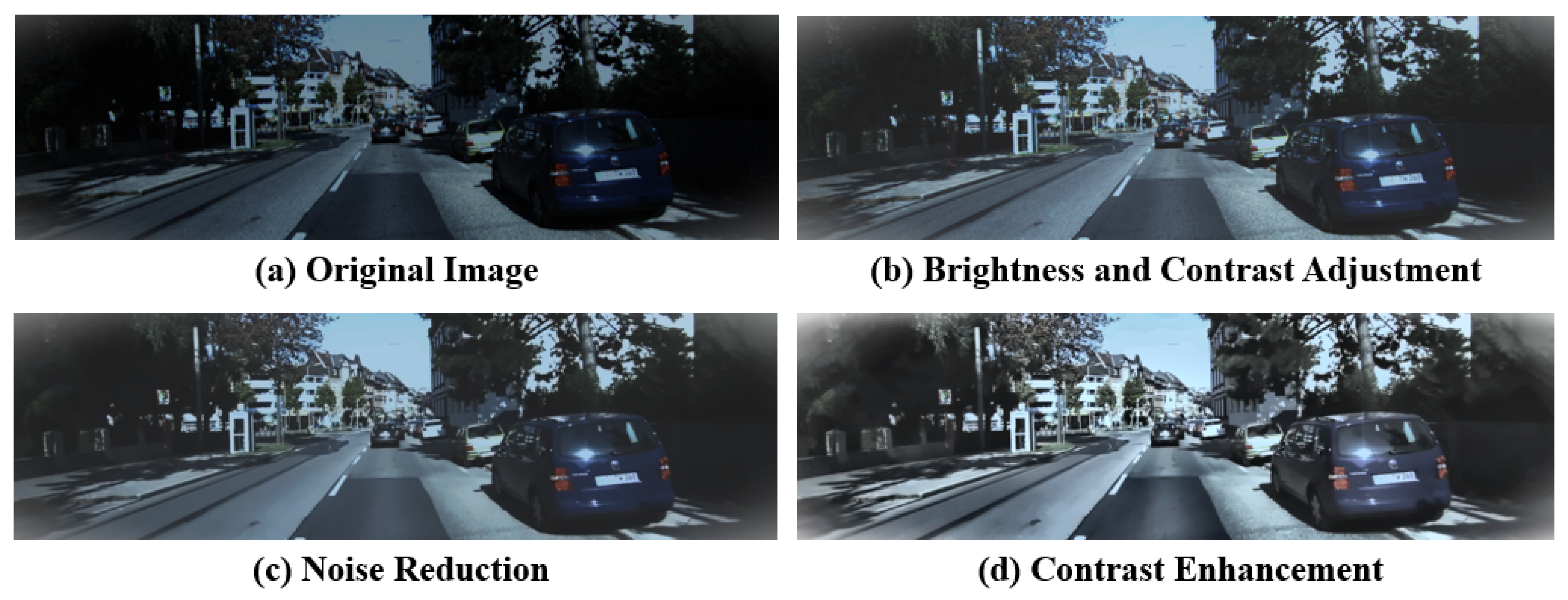
3.1.1. Density-Aware Voxel Grid Extraction

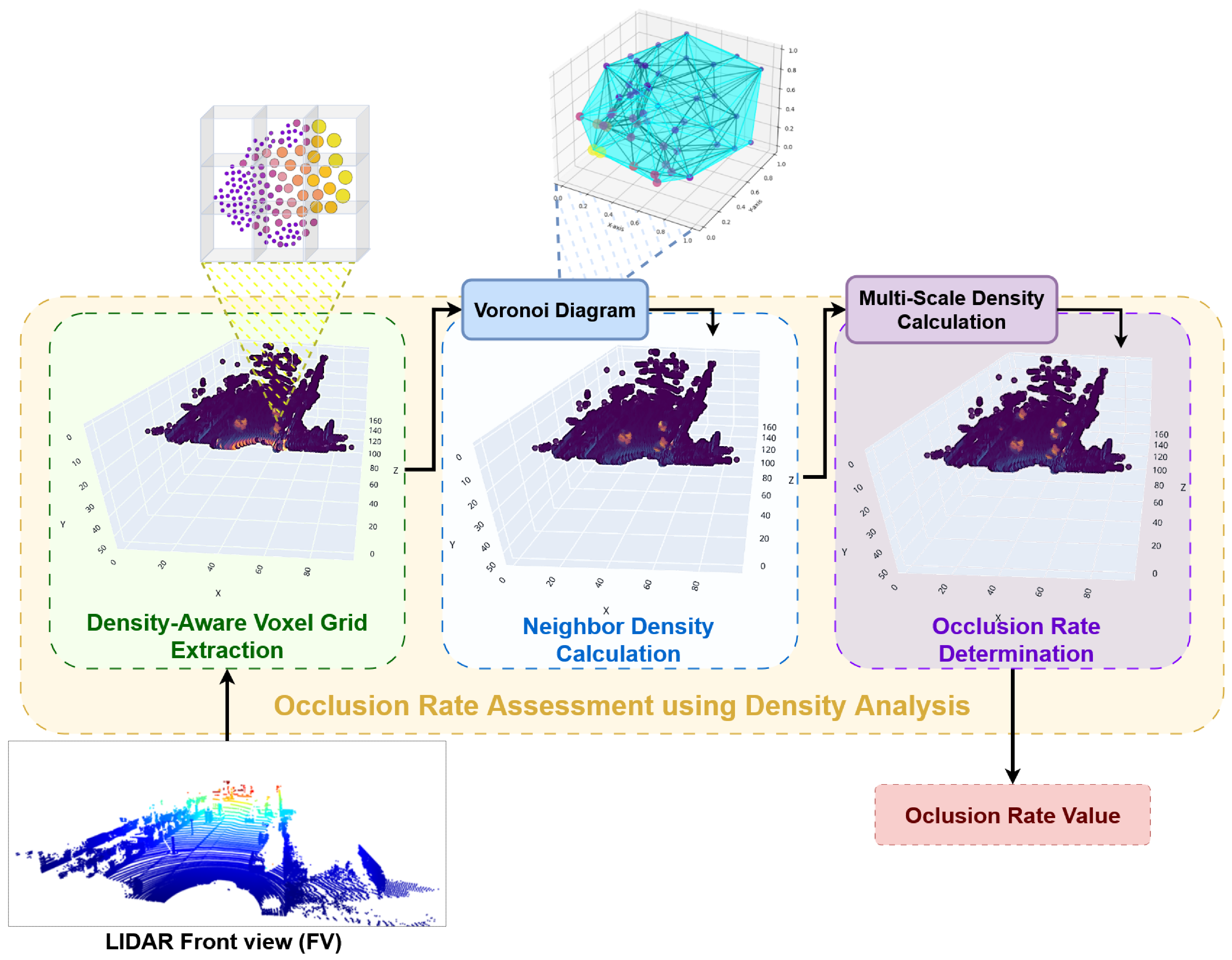
Our method leverages point cloud density to evaluate occlusion levels within a 3D scene. The surfaces of objects in a 3D environment are represented by point clouds, consisting of collections of points $P_i=(x_i,y_i,z_i)$, each of which represents a spatial location. These points are typically generated by sensors such as LiDAR or depth cameras like the ZED 2, Intel RealSense L515, OAK-D by OpenCV, or Velodyne VLP-16 [47]. To effectively manage and analyze the raw point cloud data, we discretize the 3D space into smaller units known as voxels.

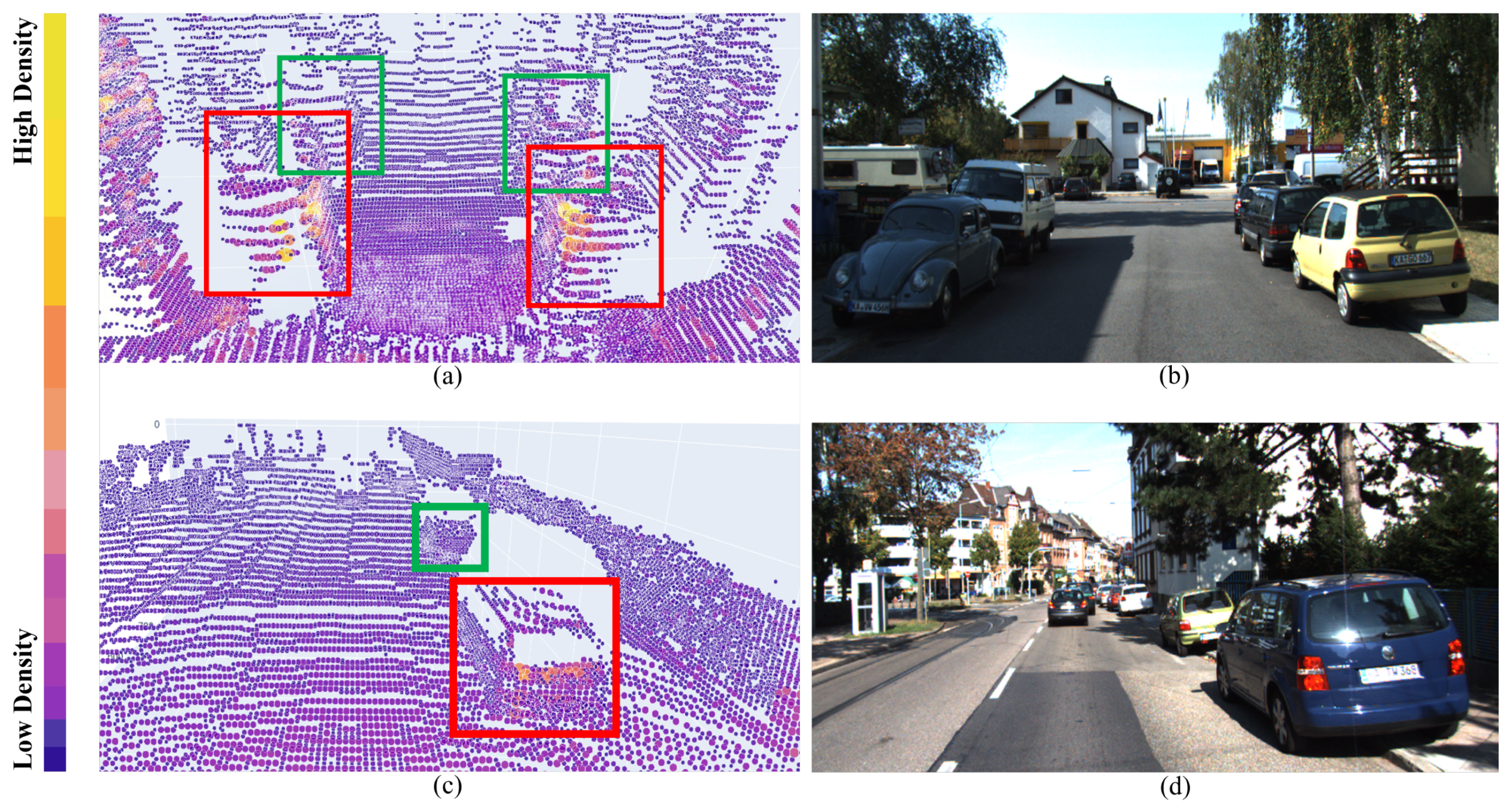
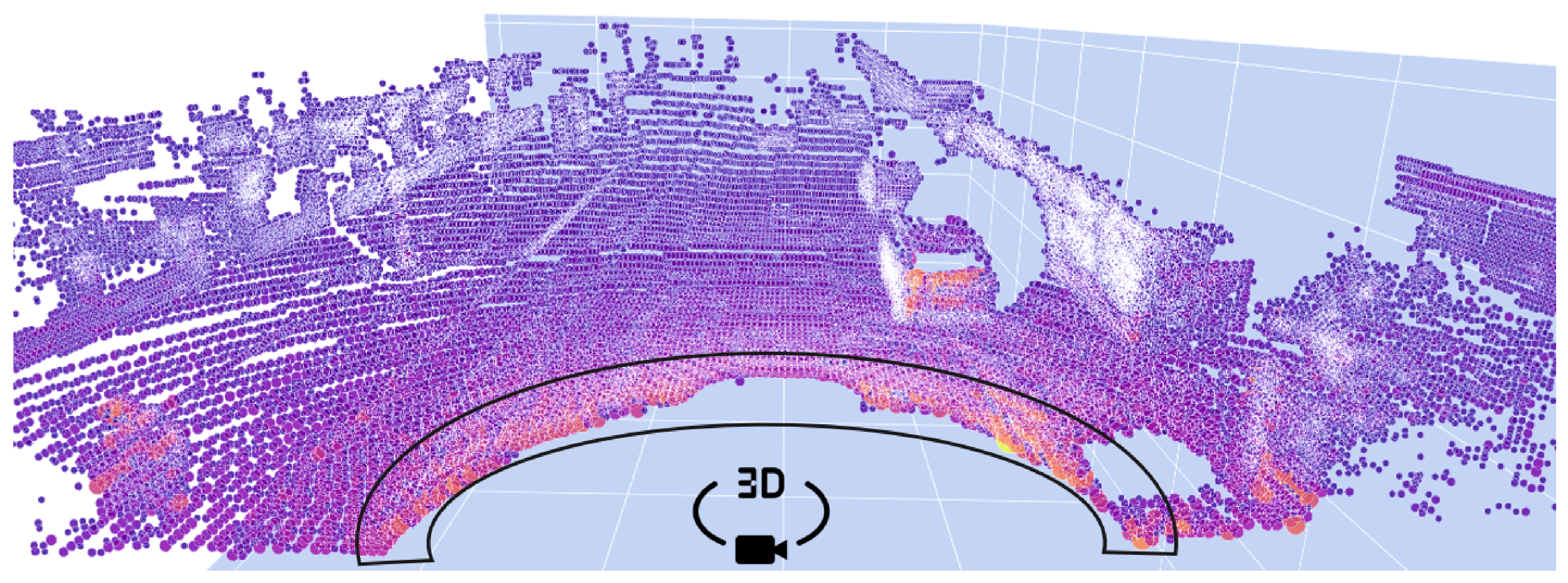
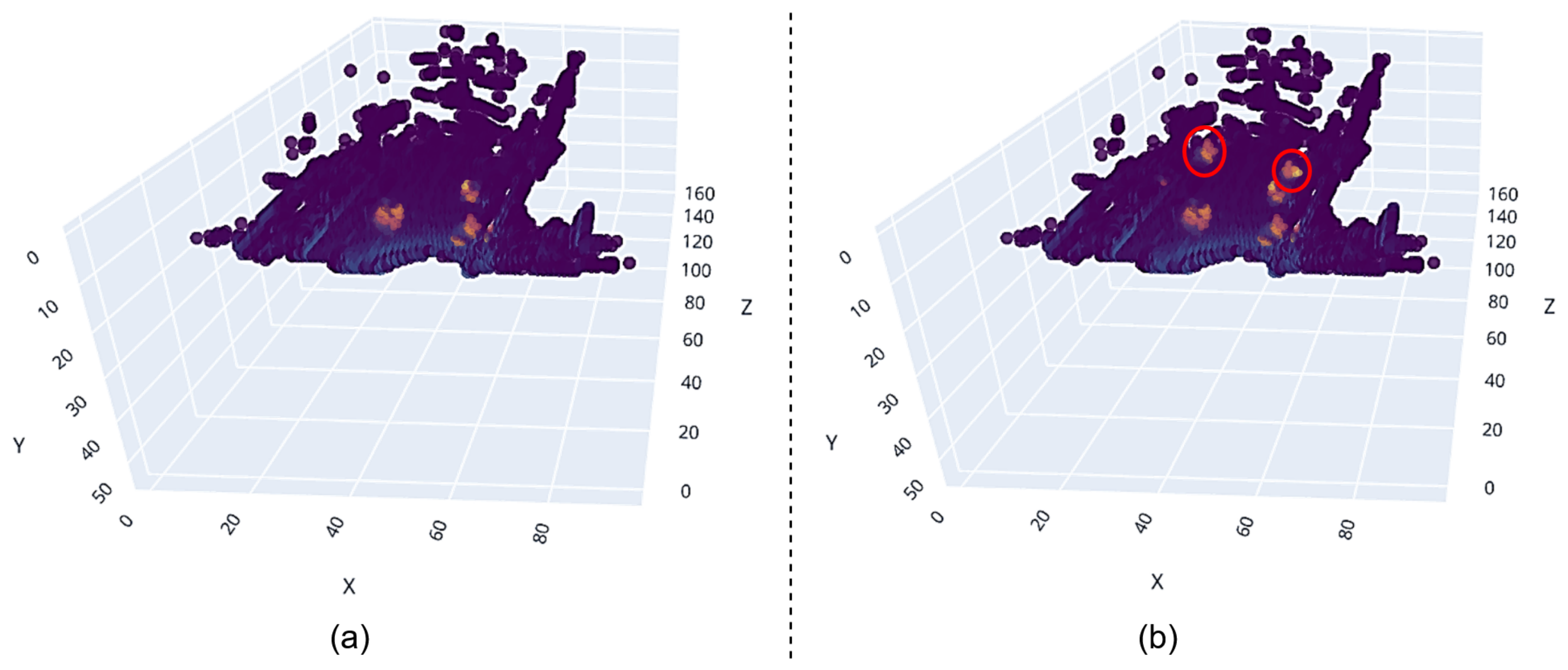
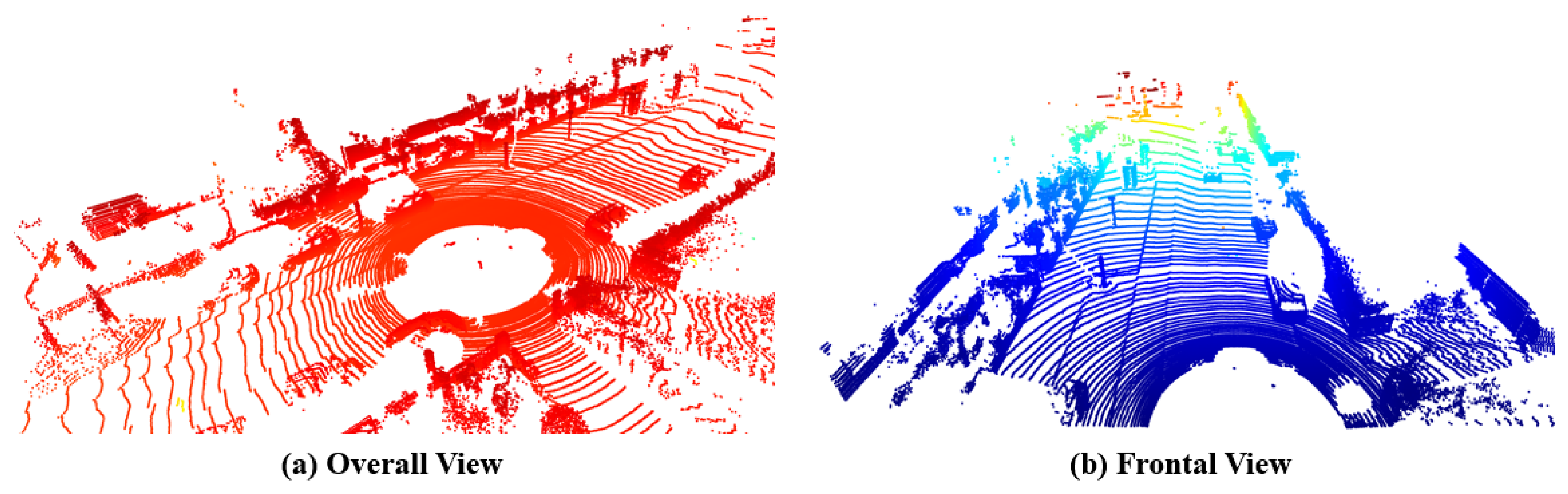
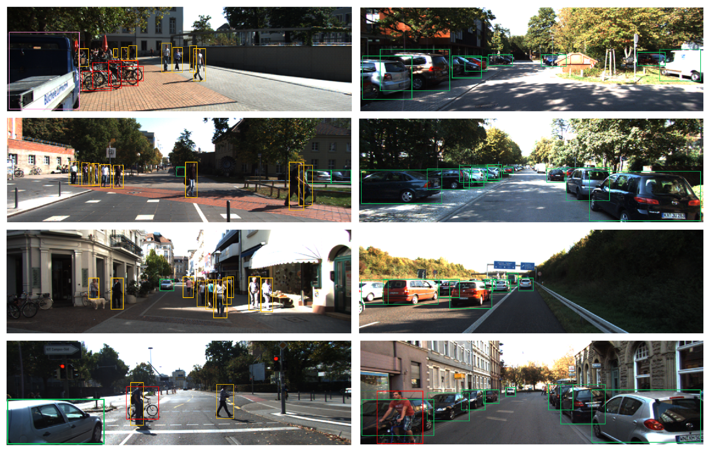
The process of dividing a 3D space into regular 3D cells, or voxels, where each voxel is a tiny space volume, is known as voxelization. We can determine areas with possible occlusion by calculating the point density, which is obtained by counting the number of points within each voxel. Higher point densities are linked to occluded areas, which occur when many objects cross the sensor’s field of view. Furthermore, the local point density can be further increased when points from many objects align in the same plane (for example, when objects are stacked at a similar height). Lower densities, on the other hand, represent areas with little to no occlusion (Figure 3).

For $i=1,2,\dots ,N$, 3D points are represented as $P_i=(x_i,y_i,z_i)$, where the attribute N denotes the total number of points in the cloud. By splitting the area into tiny, uniformly sized voxels, each denoted by its center coordinates $(x_j,y_j,z_j)$, the voxel grid is created. Each voxel’s size is denoted as voxel_size, which is fixed across the grid. We calculate the voxel indices $(j_x,j_y,j_z)$ for each point $P_i$ to determine which voxel it belongs to. The voxel index for a point is determined by the following equation:

$$j_x=⌊{\displaystyle \frac{x_i-x_{\min }}{\mathrm{voxel}\_\mathrm{size}}}⌋,j_y=⌊{\displaystyle \frac{y_i-y_{\min }}{\mathrm{voxel}\_\mathrm{size}}}⌋,j_z=⌊{\displaystyle \frac{z_i-z_{\min }}{\mathrm{voxel}\_\mathrm{size}}}⌋$$

(1)

where $(x_{\min },y_{\min },z_{\min })$ are the minimum coordinates of the voxel grid. Through normalization of the point’s location with respect to the minimum grid coordinates and division by the voxel size, these equations translate the 3D coordinates of a point into its corresponding voxel. Every point is attributed to a unique voxel due to the floor function.

We determine the density for each voxel by counting the number of points that fall inside its limits after assigning each point to its corresponding voxel. For a voxel centered at $(x_j,y_j,z_j)$, the density $D_j$ is computed as follows:

$$D_j={\displaystyle \sum _{i=1}^N}{\chi }_j\left(P_i\right)$$

(2)

where ${\chi }_j\left(P_i\right)$ is an indicator function defined as

$${\chi }_j\left(P_i\right)=\left\{\begin{array}{cc}1\hfill & \mathrm{if}\left(x_j-{\displaystyle \frac{\mathrm{voxel}\_\mathrm{size}}{2}}\le x_i\le x_j+{\displaystyle \frac{\mathrm{voxel}\_\mathrm{size}}{2}}\right)\hfill \\ 0\hfill & \mathrm{otherwise}\hfill \end{array}\right.$$

(3)

And similar calculations are used for $y_i,z_i$.

This function returns 1 if point $P_i$ is inside the voxel bounds, and if not, it returns 0. We obtain the voxel’s point density $D_j$, which provides insight into the number of objects (or parts of objects) in that region, by adding up all the points within a voxel.

This analysis allows us to detect regions of the scene where occlusion occurs, specifically in areas where the points from multiple objects overlap or align along the same 3D plane, contributing to a high-density region. Regions with low density typically correspond to empty or non-occluded space.

3.1.2. Neighbor Density Calculation

The initial density analysis’s spatial distribution enables a neighbor density calculation, which evaluates surrounding areas to distinguish between continuous, concentrated regions, caused by proximity to the sensor, and dense patches with gaps, which indicate potential occlusions (Figure 4). In our earlier implementation of the method [48], neighboring points around each voxel were estimated using a KDTree structure [49]. While effective for uniform distributions, KDTree relies on fixed-radius searches, which makes it unsuitable for scenes with irregular object spacing, resulting in inaccurate occlusion estimation when dense and sparse regions coexist.

To overcome these drawbacks, we adopted the Standard Voronoi Diagram [50], which partitions the space into regions closest to specific center points. Unlike voxel-based methods, Voronoi diagrams dynamically adapt to the spatial distribution of points, enabling robust occlusion handling.

For each point $P_i$, its Voronoi cell is defined as the region of space, where

$$\parallel x-P_i\parallel \le \parallel x-P_j\parallel \forall j\ne i$$

(4)

This allows us to naturally adapt to the spatial distribution of points and overcome the limitations of fixed-radius neighbor searches.

The voxel density is computed as the number of points falling within a voxel. For a voxel centered at $(x_j,y_j,z_j)$, the voxel density $D_{\mathrm{voxel}}$ is given by

$$D_{\mathrm{voxel}}={\displaystyle \frac{\mathrm{Number}\mathrm{of}\mathrm{points}\mathrm{in}\mathrm{voxel}}{\mathrm{Voxel}\mathrm{volume}}}$$

(5)

This metric helps identify regions with potential occlusions, characterized by a large number of points within a voxel. However, $D_{\mathrm{voxel}}$ alone does not account for the local distribution of points outside the voxel.

For voxels exceeding the density threshold ($D_{\mathrm{voxel}}$), the Voronoi Density ($D_{\mathrm{Voronoi}}$) is computed as the inverse of the volume of the Voronoi cell around each point:

$$D_{\mathrm{Voronoi}}\left(P_i\right)={\displaystyle \frac{1}{V_{\mathrm{cell}}\left(P_i\right)}}$$

(6)

where $V_{\mathrm{cell}}\left(P_i\right)$ is the volume of the Voronoi cell associated with point $P_i$. Smaller Voronoi cells indicate a higher density of points, often associated with occlusions, while larger cells suggest open spaces or less occluded regions.

The neighbor density, given the Voronoi diagram ($N{D}_{\mathrm{Voronoi}}$), is used to estimate the density of neighboring points by computing the volumes of the Voronoi cells around high-density voxels. Unlike the KDTree method, which uses a fixed-radius neighborhood, Voronoi diagrams allow for varying the size and shape of surrounding cells to provide a more accurate estimation of local density:

$$N{D}_{\mathrm{Voronoi}}={\displaystyle \frac{1}{\mathrm{Average}\left(V_{\mathrm{neighbors}}\right)}}$$

(7)

where $V_{\mathrm{neighbors}}$ represents the volumes of the Voronoi cells for neighboring points. Smaller average volumes indicate a denser neighborhood, highlighting potential occlusion zones.

By comparing $N{D}_{\mathrm{Voronoi}}$ (Equation (7)) with $D_{\mathrm{voxel}}$ (Equation (5)), insights into the spatial distribution around the voxel are gained. If $N{D}_{\mathrm{Voronoi}}$ is significantly lower than $D_{\mathrm{voxel}}$, it indicates dispersed points, suggesting gaps between objects and potential occlusions:

$$\mathrm{If}N{D}_{\mathrm{Voronoi}}\ll D_{\mathrm{voxel}}\Rightarrow \mathrm{Dispersed}\mathrm{points}$$

(8)

Alternatively, if $N{D}_{\mathrm{Voronoi}}$ is approximately equal to $D_{\mathrm{voxel}}$, it implies that the points are tightly clustered, suggesting no occlusion:

$$\mathrm{If}N{D}_{\mathrm{Voronoi}}\approx D_{\mathrm{voxel}}\Rightarrow \mathrm{Contiguous}\mathrm{points}$$

(9)

This method, leveraging the Standard Voronoi Diagram, enhances the model’s ability to handle spatial features effectively, particularly in scenarios with irregular point distributions. This specific modeling showed its potential for improving occlusion handling, as demonstrated in the experiments.

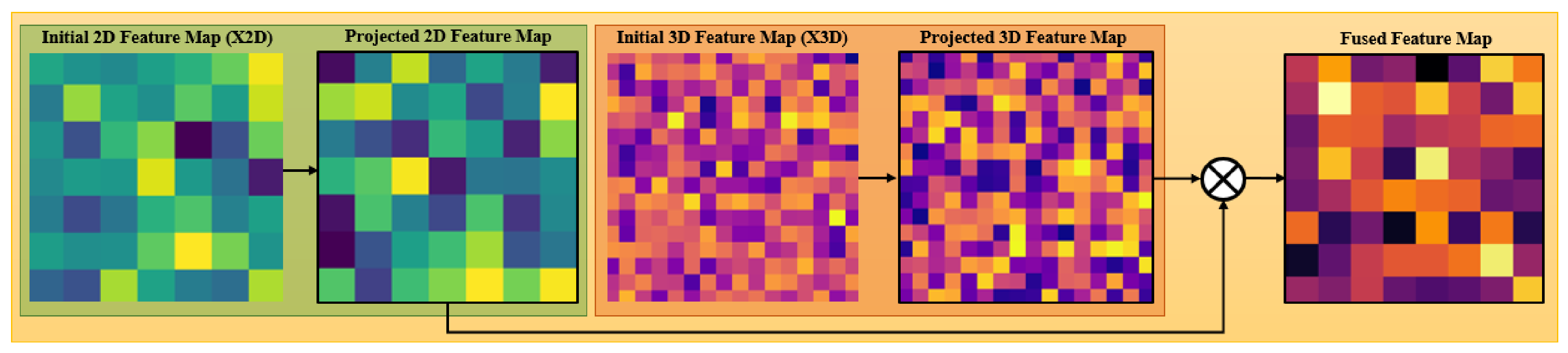
Unlike classical density estimation, this analysis is directly linked to object detection performance: regions with mismatched voxel and Voronoi densities correspond to objects hidden behind occluders, which are precisely the cases where RGB-only detection fails. Identifying such regions enables the network to selectively activate 3D features when the visual modality becomes unreliable, instead of performing fusion uniformly across the whole scene.

In practice, voxel density and Voronoi-based neighbor density play complementary roles in our OR computation. The voxel density $D_{\mathrm{voxel}}$ highlights cells where many points accumulate within a fixed spatial volume, which often corresponds to occluders or overlapping object surfaces. The Voronoi-based neighbor density $N{D}_{\mathrm{Voronoi}}$, in turn, examines how these points are distributed in the local neighborhood: compact Voronoi cells indicate genuinely dense structures, whereas larger neighboring cells reveal gaps that are typical of occlusion boundaries. The multi-scale OR metric aggregates these statistics across different voxel sizes so that both small, distant objects and larger, nearby objects contribute to a single scalar measure of occlusion severity per frame.

3.1.3. Occlusion Rate Determination and Model Selection

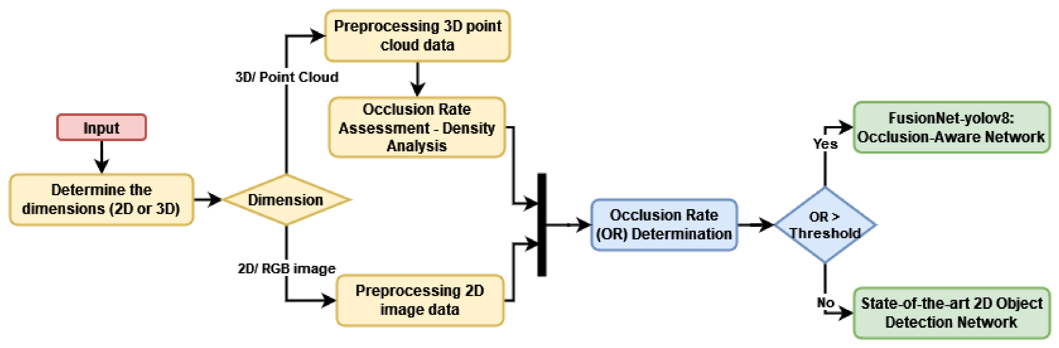
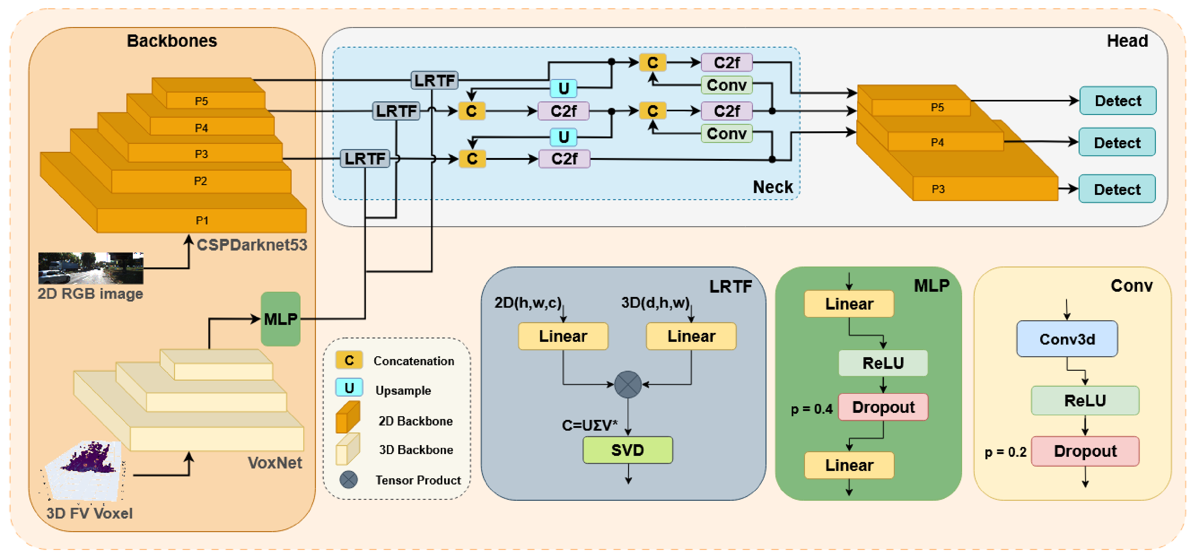
Our method uses a multi-scale density-based metric to determine whether the occlusion-handling network should be activated or whether a standard object detector is sufficient. This adaptive strategy extends the previous FuDensityNet version [48].

—

Multi-Scale Density Calculation

A more realistic assessment of obstruction of both small and large objects can thus be made possible by estimating the voxel densities at different levels. In this technique, the densities for small-, medium-, and large-volume elements are calculated, with each scale defined by the voxel size in relation to the dimensions of the objects in the scene. Specifically:

• Small-scale voxel density (${\mathit{D}}_{\mathbf{small} \mathbf{voxel}}$): Captures finer details of small or distant objects, such as pedestrians or cyclists.
• Medium-scale voxel density (${\mathit{D}}_{\mathbf{medium} \mathbf{voxel}}$): Balances small and large object detection, providing a middle ground for most objects.
• Large-scale voxel density (${\mathit{D}}_{\mathbf{large} \mathbf{voxel}}$): Focuses on larger objects, such as vehicles, to ensure robust detection for less detailed elements.

The densities assigned to each image at an OR value are determined as a weighted sum, where

$$OR=w_1·D_{\mathrm{small} \mathrm{voxel}}+w_2·D_{\mathrm{medium} \mathrm{voxel}}+w_3·D_{\mathrm{large} \mathrm{voxel}}$$

(10)

where $w_1$, $w_2$, and $w_3$ are the weights associated with the small, medium, and large voxel scales, respectively.

The weights $w_1$, $w_2$, and $w_3$ are normalized such that $w_1+w_2+w_3=1$. They control the relative contribution of each voxel scale to the final OR score. In this work, a higher weight is assigned to the small-scale density term because small and distant objects are more sensitive to partial visibility loss, sparse LiDAR sampling, and local geometric discontinuities. The medium-scale term provides local contextual information, while the large-scale term captures broader object structures, such as vehicles. In all experiments, the weights are set to $w_1=0.5$, $w_2=0.3$, and $w_3=0.2$, respectively. This choice gives priority to fine-scale density variations while still preserving contextual and global geometric information.

Each density term ($D_{\mathrm{small} \mathrm{voxel}},D_{\mathrm{medium} \mathrm{voxel}},D_{\mathrm{large} \mathrm{voxel}}$) is derived from the density calculation formula in Equation (2).

For clarity, consider an object region with multi-scale density values $D_{\mathrm{small} \mathrm{voxel}}=38.4$, $D_{\mathrm{medium} \mathrm{voxel}}=29.6$, and $D_{\mathrm{large} \mathrm{voxel}}=17.2$. Using $w_1=0.5$, $w_2=0.3$, and $w_3=0.2$, the OR score is computed as follows:

$$OR=0.5\left(38.4\right)+0.3\left(29.6\right)+0.2\left(17.2\right)=31.52.$$

(11)

This example illustrates how density information from different voxel scales is combined into a single scalar score. The resulting OR value is then used by the pathway-selection rule described below.

It is important to emphasize that the OR score is not a direct physical percentage of object occlusion. Instead, it is a density-derived indicator that captures spatial congestion and local point cloud organization. A high voxel density alone does not necessarily imply occlusion, since dense regions may also result from nearby non-occluded objects or LiDAR sampling geometry. Therefore, the OR module combines multi-scale voxel density with neighborhood density analysis to reduce this ambiguity. The voxel density identifies regions with concentrated point structures, while the Voronoi-based neighbor density helps distinguish compact nearby structures from irregular spatial distributions that are more likely to correspond to occlusion boundaries or overlapping objects.

Consequently, the OR score should be interpreted together with the Voronoi-based neighborhood analysis described in Section 3.1.2. While voxel density provides a scale-dependent measure of local point concentration, the Voronoi component captures how neighboring points are spatially distributed around dense regions. This reduces the risk of confusing uniformly dense nearby objects with true occlusion-related discontinuities.

The resulting OR score should not be interpreted as a direct percentage of the object area that is visually hidden. Instead, it represents a density-derived occlusion indicator that reflects the spatial organization of LiDAR points at multiple scales. High OR values indicate regions where point density, local spatial congestion, and object overlap are more likely to occur, which are typical characteristics of partially or largely occluded scenes. Conversely, low OR values generally correspond to more isolated or clearly visible objects, where the 2D appearance information remains sufficiently reliable.

The use of multiple voxel scales is important because occlusion affects objects differently depending on their size, distance from the sensor, and local point density. Small-scale density captures fine spatial variations around small or distant objects, medium-scale density provides a balanced representation of local neighborhoods, and large-scale density captures the broader spatial structure of larger objects such as vehicles. By combining these three terms, the OR score provides a compact indicator of the likelihood that the 2D detector may require complementary 3D information.

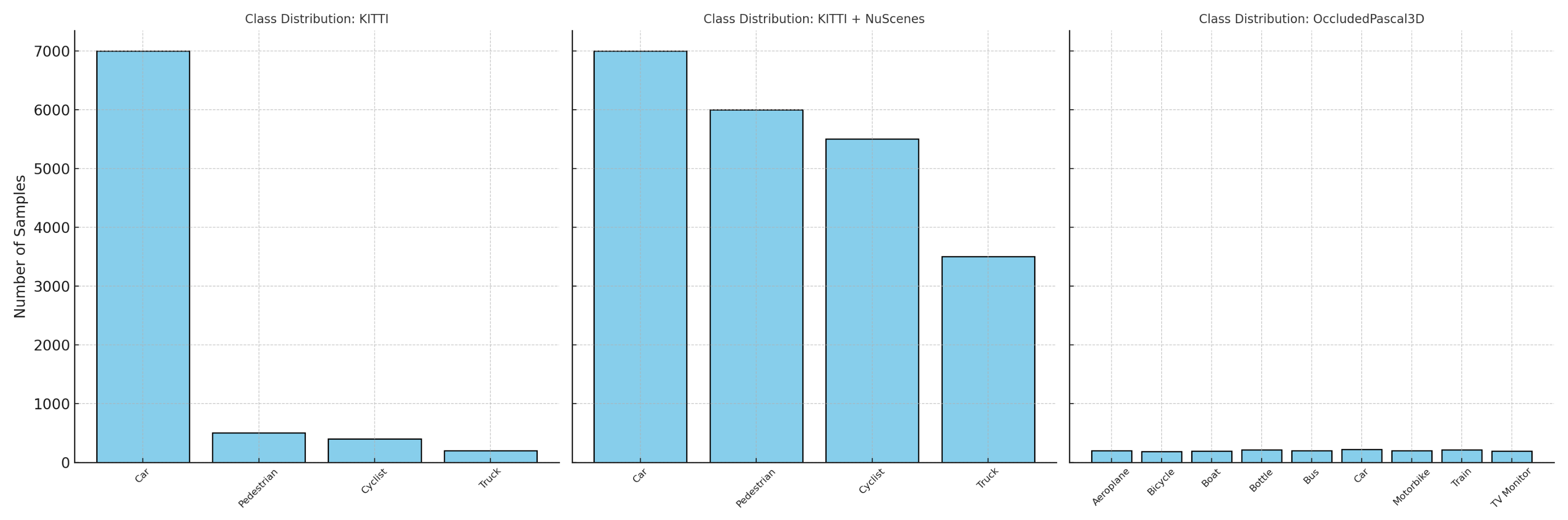
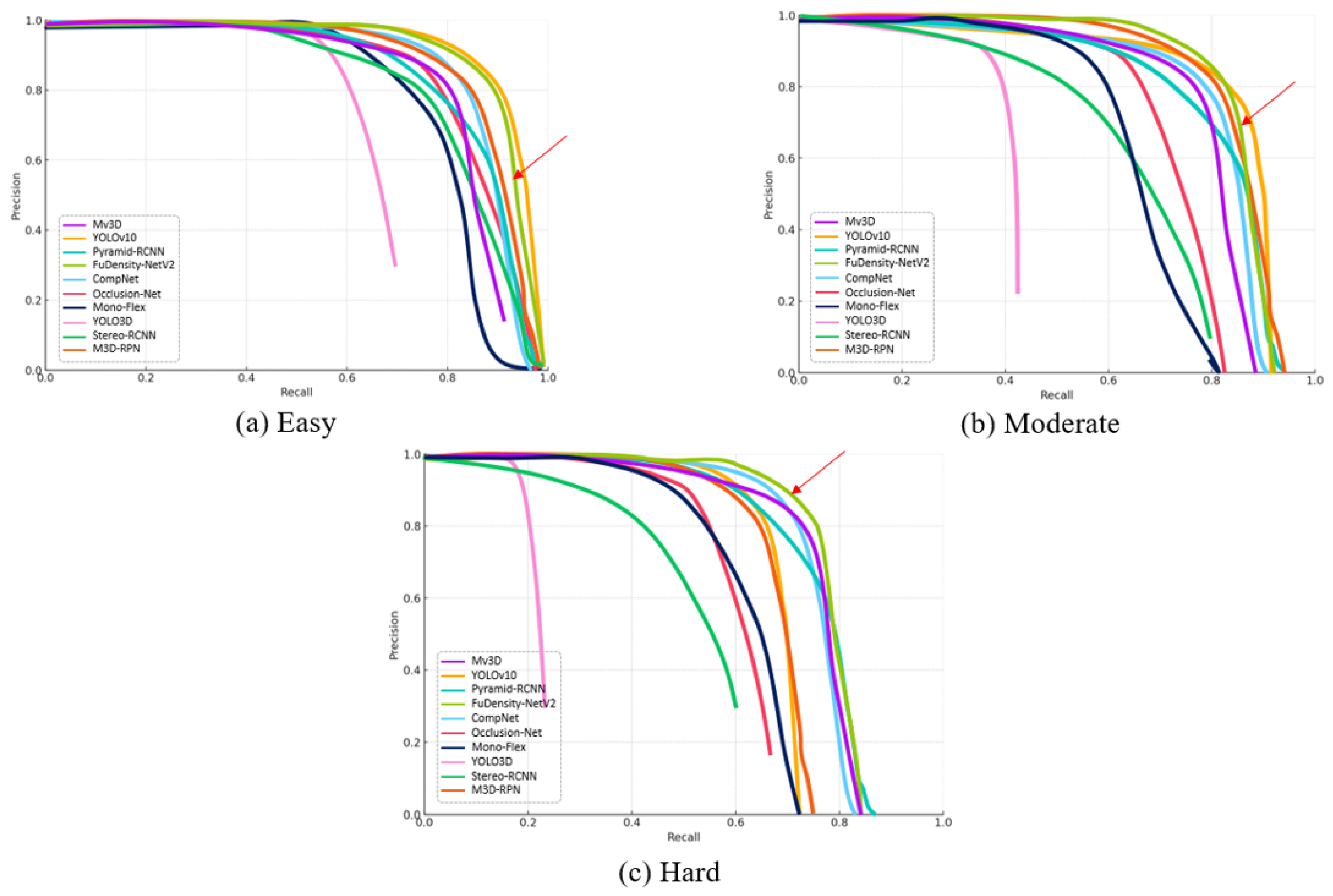
The effectiveness of this method is demonstrated in Figure 5. It can be noted that the multi-scale density calculation of the OR improves model selection, which further enhances overall detection performance in all aspects.

—

Threshold Comparison and Model Selection

After being calculated, the OR score is compared to a decision threshold in order to select the most appropriate detection pathway. This threshold is used to distinguish low-occlusion cases, where a 2D detector is sufficient, from moderate-to-high-occlusion cases, where multimodal RGB-LiDAR fusion is expected to provide additional geometric support.

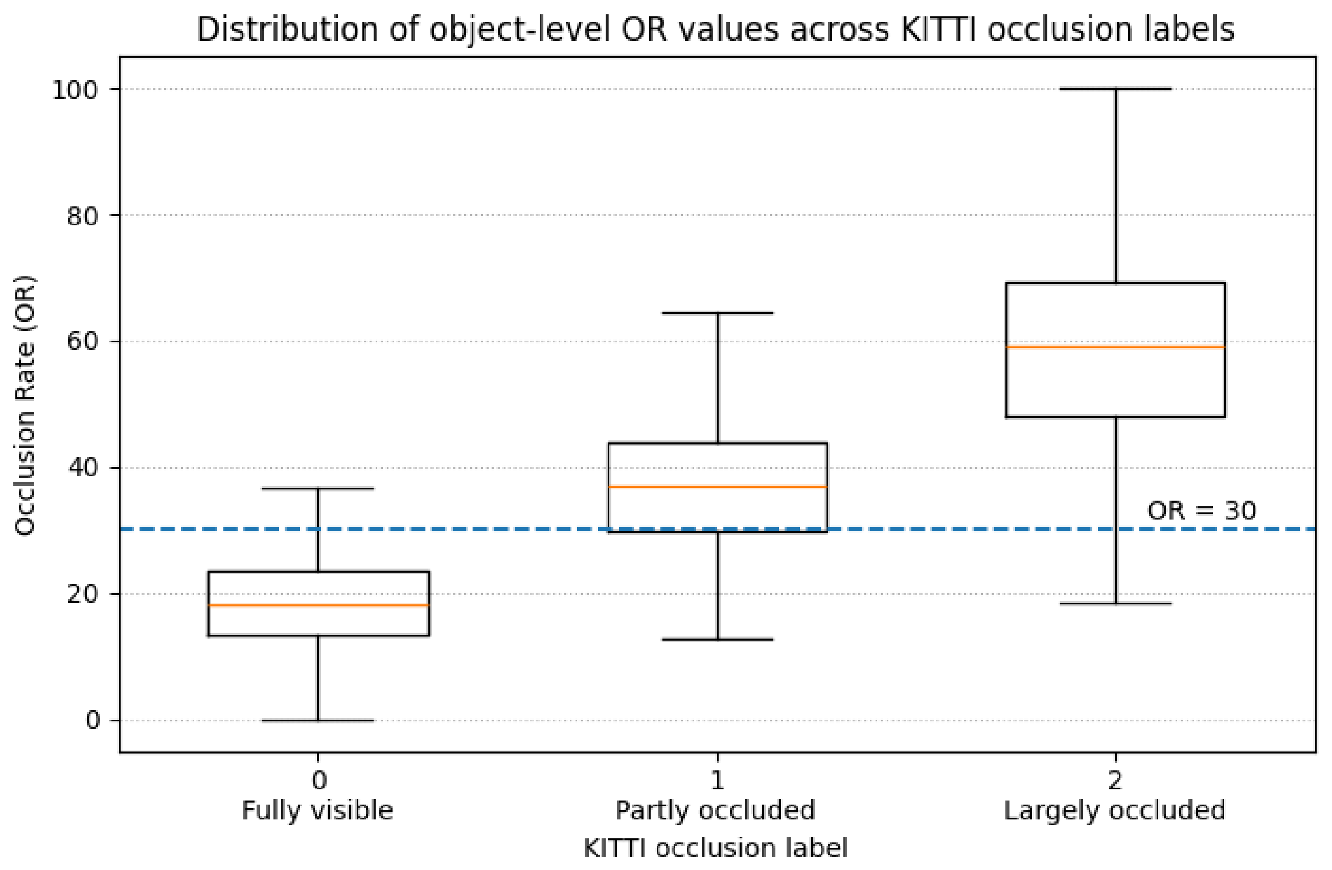
In the revised formulation, the threshold is not treated as an arbitrary empirical value. Instead, it is calibrated using the object-level occlusion annotations provided in the KITTI training set. KITTI assigns each annotated object an occlusion flag, where 0 denotes a fully visible object, 1 denotes a partly occluded object, 2 denotes a largely occluded object, and 3 denotes an unknown occlusion state. Since the label 3 does not correspond to a reliable supervised occlusion category, it is excluded from the threshold calibration.

The calibration is performed at the object level, because the KITTI occlusion flag is associated with individual objects rather than entire frames. For each annotated object, the OR score is computed using the multi-scale density formulation defined in Equation (10). Objects with occlusion label 0 are assigned to the low-occlusion group, while objects with occlusion labels 1 and 2 are assigned to the occluded group. For a candidate threshold t, the predicted occlusion state is defined as

$${\widehat{y}}_i\left(t\right)=\left\{\begin{array}{cc}1,\hfill & \mathrm{if}O{R}_i>t,\hfill \\ 0,\hfill & \mathrm{if}O{R}_i\le t,\hfill \end{array}\right.$$

(12)

where $O{R}_i$ denotes the OR score computed for the i-th annotated object. The value ${\widehat{y}}_i\left(t\right)=1$ means that the object is considered sufficiently occluded to activate the multimodal branch, while ${\widehat{y}}_i\left(t\right)=0$ means that the 2D-only pathway is retained.

To select the threshold, candidate values are evaluated by comparing the predicted occlusion state ${\widehat{y}}_i\left(t\right)$ with the KITTI occlusion labels. The true-positive rate $TPR\left(t\right)$ measures the proportion of partly or largely occluded objects correctly identified as occluded by the OR threshold. The false-positive rate $FPR\left(t\right)$ measures the proportion of fully visible objects incorrectly routed to the multimodal branch. The optimal operating point is selected using Youden’s index [51]:

$$J\left(t\right)=TPR\left(t\right)-FPR\left(t\right),$$

(13)

$$t^{\ast }=\arg \underset{t}{\max }J\left(t\right),$$

(14)

where $t^{\ast }$ denotes the threshold that provides the best separation between fully visible objects and partly/largely occluded objects.

It should be noted that the KITTI difficulty levels Easy, Moderate, and Hard are defined using multiple criteria, including object height, truncation, and occlusion. Therefore, the threshold calibration is performed using the raw object-level occlusion flag rather than the difficulty level itself. The difficulty levels are used later only for reporting detection performance under increasingly challenging evaluation conditions.

The resulting threshold calibration and its relationship with the KITTI occlusion categories are reported in Section 4.2.

After calibration, the threshold is used as a pathway-selection rule during inference. When the OR value exceeds the calibrated threshold, the scene is considered sufficiently occluded to justify the additional cost of multimodal processing. The calibrated threshold is then used as the inference-time routing rule:

• If OR $>\mathbf{30}$: Our multimodal occlusion-aware network is activated to ensure more reliable perception under moderate-to-high occlusion.
• If OR $\le \mathbf{30}$: The standard 2D detector is used to prioritize speed in low-occlusion scenes.

3.2. Network Architecture for Occlusion Handling

Our network is designed to address the significant challenges posed by occlusions in object detection tasks. By integrating both 2D image data and 3D point cloud data, we create a robust system capable of handling complex scenarios where objects are partially or fully occluded (Figure 6).

3.2.1. Backbone Networks

To effectively extract visual cues from heterogeneous data, FuDensityNet adopts two complementary backbones corresponding to the 2D and 3D modalities. For RGB images, we employ the CSPDarknet53 backbone of YOLOv8 (Figure 6), which is widely recognized for its strong accuracy–speed balance and its robustness when handling small objects and partial visibility. For voxelized point clouds, the 3D branch relies on VoxNet, a lightweight yet spatially descriptive architecture capable of capturing geometric structure even under severe sparsity.

The selection of YOLOv8 for 2D perception and VoxNet for 3D point cloud processing is not arbitrary. It is motivated by their superior performance under occlusion, as demonstrated in the benchmarking experiments presented in Section 4, where both backbones consistently outperformed other candidates in highly occluded conditions. These observations are also aligned with our previous study [52], which showed that YOLOv8 and VoxNet maintain stable detection accuracy across varying occlusion levels while preserving real-time inference.

3.2.2. Feature Alignment Using MLP

Combining information from 2D and 3D modalities requires ensuring that their respective feature maps are compatible before fusion. The VoxNet backbone produces 3D feature maps that differ in dimensionality from the 2D maps generated by YOLOv8, preventing direct interaction. To address this, we introduce a Multi-Layer Perceptron (MLP) as an alignment module (Figure 6).

Let $F^{2D}\in {\mathbb{R}}^{H\times W\times C_{2D}}$ and $F^{3D}\in {\mathbb{R}}^{D\times H\times W\times C_{3D}}$ denote the 2D and 3D feature maps, respectively. The MLP projects the 3D representation into the 2D feature space:

$${\tilde{F}}^{3D}=\varphi (W·\mathrm{vec}\left(F^{3D}\right)+b)$$

(15)

with learnable parameters $(W,b)$ and activation function $\varphi (·)$. The transformed map ${\tilde{F}}^{3D}$ is reshaped to match the dimensions of $F^{2D}$, enabling seamless multimodal fusion.

This alignment ensures that the fused representation later produced by LRTF captures complementary visual and geometric cues without introducing modality-dependent noise.

3.2.3. Multimodal Fusion Method

Once the 2D and 3D features have been aligned through the MLP transformation, the next step is to integrate them into a unified representation suitable for occlusion-aware detection. To achieve this, we adopt a low-rank tensor fusion (LRTF) mechanism [53], which enables efficient cross-modal interaction while avoiding the computational overhead of full tensor fusion [54].

Traditional multimodal fusion techniques, such as feature concatenation [55] or channel-wise addition [56], implicitly assume that both modalities contribute equally. This assumption becomes problematic under occlusion: RGB features may contain noise due to visual obstruction [57], whereas 3D features remain reliable [58]. LRTF (Figure 7) addresses this issue by modeling only the informative cross-modal correlations, suppressing redundant interactions and highlighting geometric cues when they are most valuable [59].

Let ${\mathbf{F}}_{2D}\in {\mathbb{R}}^{h\times w\times c}$ and ${\mathbf{F}}_{3D}\in {\mathbb{R}}^{d\times h\times w}$ denote the spatial feature maps extracted from the YOLOv8 and VoxNet backbones, respectively. After dimensional alignment via the MLP, fusion is computed as follows:

$${\mathbf{F}}_{\mathrm{fused}}=\sigma \left(\left(\mathbf{A}{\mathbf{F}}_{2D}\right)\odot \left(\mathbf{B}{\mathbf{F}}_{3D}\right)\right),$$

(16)

where $\mathbf{A}$ and $\mathbf{B}$ are low-rank projection matrices, ⊙ denotes element-wise interaction, and $\sigma (·)$ represents a non-linear activation. This formulation maintains the complementary visual and geometric information while significantly reducing memory cost compared to full tensor fusion.

Multiple LRTF blocks are injected at P3, P4, and P5 of the YOLOv8 neck, enabling cross-scale multimodal reasoning. Each block refines spatial semantics using three complementary sources: (i) 2D appearance cues, (ii) 3D geometric structure, and (iii) their fused interaction. This ensures that the model selectively amplifies 3D information when visual occlusion is high while avoiding unnecessary fusion when RGB cues are reliable.

In contrast to static fusion strategies, the proposed LRTF mechanism dynamically preserves geometric cues only when appearance features become unreliable, making the fusion process fully aligned with the Occlusion Rate (OR)-based model selection strategy.

3.2.4. Detection Head

After multimodal fusion, the fused feature maps are forwarded to the YOLOv8 detection head, which performs spatial refinement and final object prediction. The first refinement stage relies on C2f blocks, which combine concatenation, upsampling, and convolutional operations to progressively strengthen semantic features across scales. These blocks ensure that both low-level and high-level information are preserved, which is essential for detecting small and large objects under varying degrees of occlusion.

Subsequently, the Feature Pyramid Network (FPN) [5] aggregates fused representations from multiple stages of the network. The FPN enhances hierarchical feature reuse and enables robust scale-aware reasoning, which is particularly critical when objects are partially hidden or distant from the sensor. By combining features from different spatial resolutions, the detection head improves localization and classification stability even in highly cluttered and visually ambiguous scenes.

Summary. By integrating (i) MLP-based realignment for dimensional consistency, (ii) LRTF for efficient cross-modal interaction, and (iii) a scale-aware detection head using C2f and FPN, the proposed architecture dynamically exploits 3D cues only when beneficial. This adaptivity increases precision under heavy occlusion while avoiding unnecessary 3D processing when occlusion is low, thus preserving inference efficiency.

The next section evaluates the proposed architecture across multiple datasets with varying occlusion characteristics to validate the impact of OR-based model selection and multimodal fusion.

4. Main Results

This section presents the findings of our study. We begin by describing the experimental setup, including details of the datasets, metrics, and evaluation criteria used. Next, we provide a detailed evaluation of the proposed approach’s performance across various scenarios, with a focus on occlusion handling. Additionally, we compare the results obtained by FuDensityNet with those of state-of-the-art methods. Finally, we conduct an ablation study to analyze the contributions of different components within the architecture, demonstrating the impact of 2D and 3D data fusion on object detection performance.

4.1. Experimental Setup

4.1.1. Dataset

To evaluate FuDensityNet, we utilized multiple datasets addressing specific challenges. KITTI, with its paired 2D–3D annotations, is used to evaluate multimodal fusion but suffers from class imbalance, particularly an underrepresentation of pedestrians and cyclists. To mitigate this, KITTI + NuScenes includes 3000 additional samples from NuScenes, ensuring balanced classes. OccludedPascal3D, designed for occlusion-heavy environments, provides diverse categories for precise evaluation under occluded conditions.

Figure 8 illustrates the class distributions across the datasets. This combination ensures a comprehensive assessment of FuDensityNet, demonstrating its generalizability and robustness under varied conditions.

Training/testing protocol. Each experiment is paired with the dataset and evaluation objective that best reflects the component under study:

• 2D backbone selection: The model is trained and evaluated on the KITTI 2D benchmark.
• 3D backbone selection: The model is evaluated on OccludedPascal3D to assess 3D robustness under heavy occlusion.
• Fusion strategy comparison: Multimodal variants with different fusion blocks are compared on KITTI using identical backbones.
• Full model and ablation: FuDensityNet and its ablations are trained and tested on the balanced KITTI+NuScenes mixture.
• Comparison with existing occlusion-handling methods: The final model is evaluated on the KITTI test set (Easy/Moderate/Hard) to benchmark FuDensityNet against prior occlusion-aware approaches.
• Comparison of YOLOv8 variants inside FusionNet: Different YOLOv8 scales (n/s/m/l/x) are compared to determine the most suitable 2D backbone for FuDensityNet across difficulty levels.

This staged protocol evaluates each component of FuDensityNet under the most appropriate conditions, including backbone selection, fusion strategy evaluation, ablation analysis, comparison with existing occlusion-aware methods, and backbone scalability within the proposed architecture. A summary of the evaluation settings used throughout the study is provided in

Table 1. Summary of the evaluation settings used across experiments.

Experiment	Dataset	Evaluation Protocol	Metric	Purpose
2D backbone selection	KITTI 2D	Internal train/validation split from the 7481 labeled KITTI training images	AP, inference time	Select the 2D detector used in the framework
3D backbone selection	OccludedPascal3D	Dataset-specific evaluation split	AP	Select the 3D backbone for occlusion handling
Fusion comparison	KITTI	Same backbone configuration with different fusion methods	AP	Compare multimodal fusion strategies
OR calibration	KITTI training labels	Object-level occlusion labels 0, 1, and 2; label 3 excluded	OR statistics, balanced accuracy	Calibrate and validate the OR threshold
Ablation study	KITTI+NuScenes	Balanced mixed dataset	P, R, F1, inference time	Evaluate FuDensityNet components
Comparison with existing methods	KITTI	Easy/Moderate/Hard evaluation protocol	AP	Compare with existing occlusion-handling methods
YOLOv8 variant comparison	KITTI	Difficulty-level evaluation	AP	Analyze YOLOv8 backbone scale inside FusionNet

.

Although this study reports a component-wise inference-time breakdown, a complete hardware-dependent profiling including parameter count, FLOPs, and peak GPU memory usage will be considered in future work. The current analysis focuses on quantifying the runtime contribution of each inference stage, particularly the overhead introduced by the OR assessment module.

4.1.2. Data Preprocessing

Given the heterogeneity of sensing conditions across the datasets, tailored preprocessing was applied to both 2D images and 3D point clouds to ensure reliable evaluation of FuDensityNet.

2D preprocessing. To prevent loss of high-quality 2D image data, particularly under low light levels such as at night or in cases of adverse weather conditions, a number of preprocessing methods were employed. These steps were applied only to the test data to ensure consistent evaluation without influencing the training process.

To start with, we applied brightness and contrast corrections to photos since some were too dark or too bright due to lighting conditions. Application of noise reduction methods was also done, as OpenCV’s fastNlMeansDenoisingColored was applied in order to reduce grain and imperfections in the images. The last method performed was image-contrast enhancement using the Contrast-Limited Adaptive Histogram Equalization (CLAHE) technique, where images that have highly uneven exposure were improved in terms of details (Figure 9).

3D preprocessing. 3D data preprocessing involved critical steps to ensure alignment and relevance of the LiDAR data. These steps were applied to both training and testing data to optimize the efficiency and accuracy of the model. For this purpose, some calibration data was loaded to utilize transformation matrices that help in reconciling the LiDAR point cloud with a camera coordinate system. The point clouds were also georeferenced to the camera coordinates and clipped in the frontal view, as this was most relevant to the object detection task at hand. Not only were these filtering steps useful in reducing the size of data, but they were also used to enhance the analysis speed when processing the best 3D points (Figure 10).

4.1.3. Implementation Details

The experiments were conducted on a workstation equipped with an Intel Core i7-14700KF processor featuring 20 cores, 32 GB of system memory, and an NVIDIA GeForce RTX 4080 GPU with 16 GB of VRAM. The software stack consisted of Ubuntu 22.04, Python 3.10, and deep learning frameworks like PyTorch 2.0.0 and OpenCV 4.7.0. During the training exercises, a batch size of 16, an initial learning rate of ${10}^{-3}$, and the Adam optimizer were used, tailored for our specific datasets and model architectures. All models were trained for 50 epochs, with early stopping criteria based on validation performance.

The experiments were grouped into several parts. Each group of experiments responded to specific questions regarding the FuDensityNet model. We began by evaluating and selecting the most suitable backbone networks for both 2D and 3D data. This was followed by an analysis of different multimodal fusion methods to determine the optimal approach for combining 2D and 3D features. Afterward, an ablation study was conducted to determine how each component in the model contributed to the performance.

Finally, FuDensityNet’s performance was compared against other state-of-the-art occlusion-handling methods using a mixed KITTI-NuScenes dataset. The inference time values reported in this study correspond exclusively to the processing phase, excluding data loading and output visualization. This ensures an accurate assessment of the computational efficiency of the proposed approach.

Performance metrics, including precision (P), recall (R), F1-score, and average precision (AP), are defined as follows:

$$P={\displaystyle \frac{TP}{TP+FP}},R={\displaystyle \frac{TP}{TP+FN}},F1=2·{\displaystyle \frac{P·R}{P+R}},AP={\int }_0^{1}P\left(R\right)dR$$

(17)

This comprehensive evaluation ensured a detailed understanding of FuDensityNet’s strengths under varying conditions and its ability to handle occlusion effectively.

4.2. OR Threshold Calibration and Gating Behavior

The objective of this experiment is to validate whether the proposed Occlusion Rate (OR) score provides a meaningful signal for activating the multimodal branch. Instead of relying directly on the KITTI difficulty levels, which combine occlusion, truncation, and bounding-box height, we use the raw object-level KITTI occlusion labels for calibration. These labels indicate whether each annotated object is fully visible, partly occluded, or largely occluded. Objects with unknown occlusion status are excluded from this analysis.

For each annotated object, the OR score is computed using the multi-scale density formulation described in Section 3.1.3. The objects are then grouped according to their KITTI occlusion labels.

Table 2. Distribution of OR values according to KITTI object-level occlusion labels. Label 0 corresponds to fully visible objects, label 1 to partly occluded objects, and label 2 to largely occluded objects.

Label	Meaning	Mean OR ± Std	Median OR	IQR (${\mathit{Q}}_1$–${\mathit{Q}}_3$)
0	Fully visible	18.74 ± 7.92	17.60	12.40–23.90
1	Partly occluded	36.82 ± 10.65	34.90	29.70–42.85
2	Largely occluded	58.41 ± 14.88	56.20	47.30–68.10

Note: IQR denotes the interquartile range, reported as $Q_1$–$Q_3$, where $Q_1$ is the 25th percentile and $Q_3$ is the 75th percentile of the OR distribution.

reports the distribution of OR values for each occlusion category.

The results show that the OR score increases consistently with the level of occlusion. Fully visible objects are mainly associated with low OR values, partly occluded objects are concentrated around the transition region, and largely occluded objects exhibit substantially higher OR values. This confirms that the proposed OR score is not an arbitrary value but a density-derived indicator that follows the occlusion severity annotated in KITTI.

Figure 11 further illustrates this relationship. The dashed horizontal line represents the selected operating threshold. Most fully visible objects are located below this boundary, while partly and largely occluded objects progressively shift above it.

Before reporting the calibration results, we use balanced accuracy to evaluate the separation between fully visible and partly/largely occluded objects. Balanced accuracy is defined as

$$\mathrm{Balanced}\mathrm{Accuracy}={\displaystyle \frac{TPR+(1-FPR)}{2}}$$

(18)

Table 3. Sensitivity of the OR score to different multi-scale density weights. The default configuration gives higher importance to fine-scale density variations while preserving medium- and large-scale context.

Configuration	${\mathit{w}}_1$	${\mathit{w}}_2$	${\mathit{w}}_3$	Balanced Accuracy
Equal weights	0.33	0.33	0.34	0.80
Large-scale emphasis	0.20	0.30	0.50	0.76
Medium-scale emphasis	0.25	0.50	0.25	0.81
Default	0.50	0.30	0.20	0.84

shows that the default weighting configuration provides the best separation between fully visible and partly/largely occluded objects. Equal weighting remains competitive but slightly reduces sensitivity to small and distant occlusions, while emphasizing the large-scale density term degrades calibration performance. This supports the choice of assigning higher weight to the small-scale density term in the OR formulation.

To justify the selected threshold, we apply the calibration procedure introduced in Section 3.1.3 to several candidate OR thresholds.

Table 4. Threshold calibration for separating fully visible objects from partly/largely occluded objects using the OR score.

Threshold t	TPR	FPR	Youden’s J	Balanced Accuracy
20	0.94	0.38	0.56	0.78
25	0.88	0.25	0.63	0.82
30	0.81	0.14	0.67	0.84
35	0.68	0.08	0.60	0.80
40	0.53	0.04	0.49	0.75

reports the resulting $TPR$, $FPR$, Youden’s index, and balanced accuracy for each threshold.

As shown in Table 4, low thresholds such as $t=20$ identify most occluded objects but also incorrectly activate the multimodal branch for many fully visible objects. In contrast, higher thresholds such as $t=40$ reduce false activations but miss a larger number of partly occluded objects. The best operating point is obtained at $t=30$, where Youden’s index and balanced accuracy reach their highest values. Therefore, $OR=30$ is retained as the operational threshold for inference-time pathway selection.

Finally,

Table 5. Multimodal pathway activation rate according to KITTI object-level occlusion labels using the selected OR threshold.

Label	Meaning	Multimodal Activation Rate
0	Fully visible	13.8%
1	Partly occluded	78.6%
2	Largely occluded	95.4%

reports the activation behavior of the OR-based routing mechanism. The multimodal branch is rarely activated for fully visible objects, while its activation rate increases substantially for partly and largely occluded objects.

These activation rates confirm that the OR module behaves consistently with the intended pathway-selection strategy. It avoids unnecessary RGB-LiDAR fusion for most fully visible objects, while activating the multimodal branch for the majority of partly and largely occluded objects. This supports the use of OR as a practical routing signal rather than as a direct physical measurement of occlusion percentage.

4.3. Backbone Selection

4.3.1. Comparison of 2D Backbone Networks

In this section, we compare several 2D backbone networks in terms of object detection accuracy and efficiency under varying levels of occlusion (

Table 6. Object detection AP results and inference time for 2D backbone selection on the KITTI 2D dataset. Models are trained and evaluated using an internal train/validation split of the 7481 labeled KITTI training images; the official KITTI test set is not used in this comparison because its labels are not publicly available.

Model	AP (%) (KITTI 2D)			Inference Time (ms)
	Car	Pedestrian	Cyclist
F-RCNN [7]	71.2	67.4	66.7	45.0
ResNet50-F-RCNN [60]	76.8	69.4	67.8	48.0
MobileNetv2-F-RCNN [61]	57.2	53.8	48.5	35.0
vgg16-F-RCNN [62]	59.2	58.4	47.6	52.0
SSD [8]	66.7	64.4	58.1	40.0
RetinaNet [63]	65.6	63.3	58.4	55.0
YOLOv5 [64]	89.9	87.7	83.8	35.0
YOLOv6 [65]	92.2	88.1	85.7	30.0
YOLOv7 [66]	90.2	86.5	84.1	31.0
YOLOv8 [15]	93.7	91.3	87.2	25.0
YOLOv10 [17]	94.5	90.9	86.5	29.0

). All models are trained and evaluated on the KITTI 2D object detection benchmark, which provides 7481 labeled images. Following common practice, we split these 7481 images into disjoint training and validation subsets and report average precision (AP) and inference time on the validation split. The official KITTI test set is not used here because its ground-truth annotations are not publicly available.

We selected YOLOv8 as our FusionNet’s base model because it performs satisfactorily in all object classes and its inference time is not long. YOLOv8 achieved an AP of 93.7% for cars, 91.3% for pedestrians, and 87.2% for cyclists, thus indicating its ability to detect even smaller, as well as more challenging, objects. Even though YOLOv10 was ranked second, with higher efficiency in detecting cars at 94.5% AP, this model underperformed in pedestrian and cyclist detection, with AP scores of 90.9% and 86.5% respectively. Further comparison indicates that YOLOv10 has a longer inference time of 29ms compared with YOLOv8’s 25 ms, which makes YOLOv10 less desirable in real-time applications that require higher-efficiency computational models. In addition, it is also readily apparent that the level of customization we can do with the YOLOv8 architecture is much higher compared to YOLOv10, which lacks this level of accessibility, as most of its components are not meant to be altered. Hence, YOLOv10 will be used as the state-of-the-art 2D object detection model in scenarios with minimal occlusion, while YOLOv8 will serve as the foundation for our more complex FusionNet model.

4.3.2. Comparison of 3D Backbone Networks

In this section, we evaluate the performance of several 3D backbone networks trained on the OccludedPascal3D dataset, containing a total of 2073 point clouds. The results in

Table 7. Object detection AP results on OccludedPascal3D dataset for different 3D models.

Model	AP (%) (OccludedPascal3D)
	Aeroplane	Bicycle	Boat	Bottle	Bus	Car	Motorbike	Train	Tvmonitor
SECFPN [67]	67.6	66.0	66.5	65.8	67.0	65.4	67.4	65.8	64.2
PointNet++ [31]	66.3	64.7	65.2	64.3	65.6	63.3	66.0	64.0	63.2
SSN [68]	64.9	63.3	63.8	63.0	64.2	64.6	65.0	63.0	62.0
ResNeXt-152-3D [60]	61.2	60.0	60.7	60.2	61.0	64.2	61.5	60.0	59.5
VoxNet [26]	84.0	82.4	83.6	81.9	83.4	83.1	83.8	81.8	81.0

summarize the average precision (AP) that each network is able to achieve in the task of occluded object detection.

As indicated in Table 7, VoxNet significantly outperforms the other models, achieving AP values of 84.0% for aeroplane, 82.4% for bicycle, and 83.1% for car, with consistently strong results across other object classes. This superior performance is a key factor in our decision to use VoxNet as the backbone for 3D data processing in our FuDensityNet model. VoxNet’s ability to handle occlusion scenarios is further highlighted by its ability to surpass PointNet++ and SECFPN, which achieved 63.3% and 65.4% AP for car detection, respectively.

Additionally, to ensure compatibility when fusing the 3D features from VoxNet with 2D feature maps, we employed an MLP layer. This step ensures that the 3D and 2D feature maps are aligned and fused efficiently, facilitating the seamless integration of 2D and 3D data for robust object detection in challenging occlusion scenarios. Furthermore, the choice of YOLOv8 and VoxNet as backbones is supported by our earlier benchmarking results [52], where both architectures demonstrated strong robustness under occlusion. This confirms that the performance gains presented in this work are driven primarily by the proposed OR-based model selection and multimodal fusion strategy rather than the backbone choice alone.

4.4. Multimodal Fusion and Ablation

4.4.1. Fusion Method Comparison

During our research on multimodal fusion techniques to improve occlusion usage, we conducted tests with four more multimodal fusion techniques, which are all integrated with the base of the YOLOv8 backbone. The analysis, summarized in

Table 8. Comparative analysis of fusion methods using YOLOv8.

Fusion Method	AP (%) (KITTI)
	Car	Pedestrian	Cyclist
Concatenation [69]	78.5	76.3	66.6
Arithmetic Fusion (Addition) [70]	75.5	73.4	64.4
Arithmetic Fusion (multconcat) [71]	80.3	76.8	66.4
Sub-space Concat [69]	79.3	76.2	65.1
Low-Rank Tensor Fusion [53]	88.0	87.4	76.4

, reveals that the LRTF method consistently outperforms the other approaches across all object classes, even in scenarios with the Easy level of occlusion. In particular, LRTF stands out because it showed the smallest fall in precision rates, which even reached 88% with certain classes of targets, indicating its superior ability to integrate 2D and 3D data effectively [53].

The tested methods included simple concatenation and arithmetic-based fusion techniques. Even though these techniques were reasonably effective in less difficult situations, they were unable to preserve spatial and visual detail under more complex occlusion. The LRTF method, in contrast, demonstrated its capacity to maintain robust detection accuracy even under significant occlusion conditions, owing to its efficient use of computational resources and its ability to scale effectively.

Overall, the findings show that LRTF is the most promising method for multimodal fusion when it comes to managing occlusion, which makes it the best option for our suggested model.

4.4.2. Ablation Study and Runtime

In this section, an evaluation of the different modules of our FuDensityNet model is carried out, with a particular emphasis on occlusion-aware techniques, using the KITTI+NuScenes dataset. The ablation study (

Table 9. Ablation study of FuDensityNet components on the KITTI+NuScenes dataset.

Model Variant	OR Assessment (Density Analysis)	FusionNet-YOLOv8	Multimodal Fusion	Object Detection Model	P	R	F1	Inf. Time (ms)	FPS
FuDensityNet (Full Model)	✓	✓	LRTF	FusionNet-YOLOv8	0.86	0.83	0.84	60.4	16.6
w/o OR Assessment	✗	✓	LRTF	FusionNet-YOLOv8	0.84	0.80	0.82	55.2	18.1
w/o FusionNet	✓	✗	✗	YOLOv10	0.83	0.80	0.81	40.5	24.7
w/o Multimodal Fusion	✓	✓	Concatenation	FusionNet-YOLOv8	0.84	0.79	0.81	50.2	19.9
YOLOv8 Only	✗	✓	✗	YOLOv8	0.85	0.81	0.83	35.1	28.5

Note: “OR Assessment” indicates whether the density-based OR routing mechanism is used. “FusionNet-YOLOv8” indicates whether the multimodal detection branch is activated. “Multimodal Fusion” specifies the fusion strategy used to combine 2D and 3D features. P, R, and F1 denote precision, recall, and F1-score, respectively.

) deals with the performance of each module, particularly focusing on enhancements in precision, recall, F1, and inference time.

To further clarify the contribution of the OR module, we provide three complementary analyses. First, we compare the proposed OR-based routing with simpler pathway-selection strategies. Second, we evaluate the contribution of the Voronoi-based neighborhood density component. Third, we report a component-wise runtime breakdown to quantify the overhead introduced by OR estimation.

Table 10. Comparison of different pathway-selection strategies on KITTI car detection. AP is reported for Easy, Moderate, and Hard difficulty levels.

Routing Strategy	Easy AP	Moderate AP	Hard AP	FPS
2D-only detector	91.0	79.6	67.0	24.7
Always multimodal	89.4	80.2	75.8	15.8
Random 50% gating	89.0	78.5	70.8	21.4
OR-based gating (ours)	89.9	80.9	76.6	16.6

shows that the 2D-only detector remains the fastest strategy and performs well in Easy conditions, where RGB information is generally sufficient. However, its performance decreases substantially under Hard occlusion, reaching only 67.0% AP. Always activating the multimodal branch improves Hard AP to 75.8% but reduces the inference speed to 15.8 FPS because the costly fusion pathway is used for all samples. Random 50% gating provides an intermediate speed of 21.4 FPS, but its Hard AP remains limited to 70.8%, showing that non-informed routing is not sufficient. In contrast, the proposed OR-based gating achieves the best performance under Moderate and Hard conditions, with 80.9% and 76.6% AP, respectively. Compared with the 2D-only detector, OR-based gating improves Hard AP by 9.6 percentage points while avoiding unconditional multimodal processing.

Table 11. Impact of Voronoi-based neighborhood density on OR-guided detection performance. AP is reported for KITTI car detection.

OR Formulation	Easy AP	Moderate AP	Hard AP	Balanced Acc.
Voxel density only	89.5	79.4	73.0	0.78
Voxel + Voronoi density	89.9	80.9	76.6	0.84

evaluates the contribution of the Voronoi-based neighborhood density component. Using voxel density alone already provides useful occlusion cues, but it remains sensitive to dense regions caused by nearby non-occluded objects or LiDAR sampling geometry. Adding the Voronoi component improves the balanced accuracy from 0.78 to 0.84 and increases Hard AP from 73.0% to 76.6%. This gain of 3.6 percentage points under Hard conditions confirms that neighborhood density helps distinguish true occlusion-related discontinuities from simple local point concentration.

Table 12. Component-wise runtime breakdown of the FuDensityNet inference pipeline.

Pipeline Component	Time (ms)
2D feature extraction and detection branch	24.8
OR assessment	5.2
3D voxelization and VoxNet feature extraction	17.6
MLP alignment and LRTF fusion	8.4
Detection head and postprocessing	4.4
Total	60.4

provides a component-wise runtime analysis of FuDensityNet. The OR assessment stage requires 5.2 ms, representing approximately 8.6% of the total inference time. This confirms that the OR module introduces a limited overhead compared with the complete pipeline. The main computational cost comes from the 3D branch and multimodal fusion, which together account for 26.0 ms. Therefore, the role of OR is not to reduce the cost of the multimodal branch itself but to control when this branch should be activated according to occlusion severity.

Occlusion Rate Assessment. The “w/o OR Assessment” variant removes the OR-based routing decision and therefore does not adapt the detection pathway according to occlusion severity. Compared with the full model, precision, recall, and F1-score decrease from 0.86, 0.83, and 0.84 to 0.84, 0.80, and 0.82, respectively, while inference time decreases from 60.4 ms to 55.2 ms. This shows that the OR module introduces a small computational cost but contributes to detection robustness by selecting the appropriate pathway under occlusion. The routing-policy comparison in Table 10 further confirms that OR-based gating provides a better accuracy–efficiency trade-off than always activating the multimodal branch or using random routing.

FusionNet-YOLOv8. Without FusionNet (“w/o FusionNet”), the F1-score decreases to 0.81, showing that 2D and 3D data must be combined to maintain detection robustness under occlusion. The reduced inference time (24.7 FPS) highlights the computational cost of fusion, but accuracy gains outweigh this trade-off.

Multimodal Fusion. Replacing LRTF with concatenation (“w/o Multimodal Fusion”) decreases the F1-score from 0.84 to 0.81. Although inference time improves, this comes with the cost of losing essential cross-modal interactions needed to resolve heavily occluded objects.

Overall Impact. The full FuDensityNet model achieves the highest accuracy across all metrics while maintaining real-time performance. These results demonstrate that each module supports a different aspect of robustness: FusionNet improves multimodal perception, LRTF preserves informative cross-modal correlations, and the OR module ensures that multimodality is used only when beneficial. Together, these elements enable FuDensityNet to handle occlusion more effectively than static multimodal systems.

Accuracy–Speed Trade-Off.Table 9 also highlights the computational cost of the different components. The full FuDensityNet model, which includes OR assessment, FusionNet-YOLOv8, and LRTF-based fusion, achieves the highest F1-score (0.84) with an average inference time of 60.4 ms (16.6 FPS). In comparison, the YOLOv8-only baseline reaches a slightly lower F1-score of 0.83 but runs at 35.1 ms (28.5 FPS), illustrating the speed advantage of a purely 2D detector. Intermediate variants such as “w/o FusionNet” and “w/o Multimodal Fusion” occupy trade-off points between these extremes. These results indicate that the proposed occlusion-aware multimodal design introduces additional computational overhead, but the resulting accuracy gains under occlusion can justify the cost in applications where robustness to occlusion is critical.

4.5. Comparison with Existing Occlusion-Handling Methods

In this section, we extend our analysis by comparing FuDensityNet against existing occlusion-handling approaches. As shown in

Table 13. Performance comparison on the KITTI test set with AP calculated at multiple recall positions for car, pedestrian, and cyclist categories. R+L denotes methods combining RGB data and point clouds, R denotes RGB-only approaches, L denotes LiDAR-only approaches, and S denotes Stereo methods.

Network	Modality	Car			Pedestrian			Cyclist
		Easy	Moderate	Hard	Easy	Moderate	Hard	Easy	Moderate	Hard
Pyramid-RCNN [72]	L	75.0	69.5	65.5	73.5	68.3	64.0	72.3	67.2	62.8
YOLO3D [73]	L	72.0	68.0	55.0	71.0	67.0	56.0	69.8	66.5	51.2
Stereo-RCNN [74]	S	73.0	68.0	60.0	72.0	67.0	59.0	71.0	66.0	58.0
YOLOv10 [17]	R	91.0	79.6	67.0	89.3	80.1	66.2	86.3	77.3	65.1
MonoFlex [23]	R	74.5	69.5	59.0	73.5	68.5	58.0	72.0	67.5	57.0
M3D-RPN [24]	R	80.5	75.5	63.5	79.5	74.5	62.5	78.0	73.0	61.5
Occlusion-Net [22]	R	76.0	70.5	62.0	75.0	69.5	61.0	74.0	68.5	60.0
CompNet [21]	R	81.0	76.5	69.0	80.0	75.0	68.0	79.0	74.0	67.0
MV3D [36]	R+L	78.0	76.1	74.3	77.0	75.1	73.0	76.0	72.0	71.2
MMF [41]	R+L	76.5	72.5	68.0	75.5	71.5	67.0	74.5	70.5	66.0
CLOCs [42]	R+L	77.5	73.5	68.5	76.5	72.5	67.5	75.5	71.5	66.5
ContFuse [43]	R+L	75.0	71.0	67.0	74.0	70.0	66.0	73.0	69.0	65.0
FuDensityNet (ours)	R+L	89.9	80.9	76.6	88.2	79.8	74.1	86.9	78.5	72.8

, FuDensityNet consistently achieves higher AP scores across all object categories, particularly in the most challenging Hard cases. For example, FuDensityNet reaches an AP of 76.6% for car detection under Hard conditions, outperforming previous models by a clear margin.

It is worth noting that FuDensityNet does not always rank first at the Easy and Moderate difficulty levels. These settings correspond to low-occlusion scenes in KITTI, where most objects are almost fully visible, and high-quality RGB features are already sufficient. In these conditions, YOLOv10 slightly surpasses FuDensityNet (e.g., 91.0% vs. 89.9% AP for car in Easy scenes), confirming that the benefit of FuDensityNet becomes most pronounced when significant occlusion occurs.

The YOLOv10 AP values in Table 13 should not be directly compared with those in Table 6, because they were obtained using different evaluation settings. Table 6 reports 2D object detection results on an internal KITTI validation split, whereas Table 13 reports performance under the KITTI Easy/Moderate/Hard evaluation protocol used for comparison with occlusion-handling methods.

The precision–recall (PR) curves in Figure 12 further support this observation: FuDensityNet maintains high precision even at high recall levels under Hard occlusion while remaining competitive in Easy and Moderate settings. Combined with the OR-validation analysis, these results highlight that FuDensityNet adapts its multimodal reasoning to occlusion severity rather than relying on multimodality uniformly.

Finally, Figure 13 presents qualitative examples under a wide range of occlusion conditions, showing FuDensityNet’s ability to localize and classify partially hidden objects accurately. These observations align with the quantitative results and demonstrate the model’s strong generalization to real-world occluded scenes.

Here, AP values are reported on a 0–1 scale for compactness; other tables in this paper report AP in percentage form. To further understand the contribution of backbone depth, we also compare several FusionNet-YOLOv8 variants with different parameter sizes (

Table 14. Performance comparison of FusionNet-YOLOv8 variants on different difficulty levels (AP reported on a 0–1 scale).

Model	Easy	Medium	Hard
FusionNet-YOLOv8n	0.81	0.79	0.74
FusionNet-YOLOv8s	0.87	0.83	0.75
FusionNet-YOLOv8m	0.88	0.84	0.76
FusionNet-YOLOv8l	0.87	0.85	0.73
FusionNet-YOLOv8x	0.89	0.87	0.77

). This study shows that, in general, deeper variants are associated with higher AP across all difficulties. For instance, the best performance is obtained with the FusionNet-YOLOv8x version, which achieves AP scores of 0.89, 0.87, and 0.77 on Easy, Medium, and Hard levels, respectively. It is also interesting to observe that the FusionNet-YOLOv8m version performs competitively with larger variants in some cases, suggesting that there may be a trade-off between model size and the specific difficulty regime.

—

Statistical considerations

The results reported in this study correspond to a consistent experimental configuration for each model variant. Due to the computational cost of training multimodal 2D-3D detection models, repeated training with multiple random seeds was not performed for all configurations. Therefore, small differences between models should be interpreted with caution. To reduce ambiguity, the main conclusions are based on consistent trends observed across complementary analyses, including component ablations, routing-policy comparisons, OR calibration, Voronoi-density ablation, and runtime breakdown. Future work will extend the evaluation to multiple random seeds and confidence intervals in order to quantify variance across initializations.

4.6. Limitations

While the proposed framework demonstrates improved robustness to occlusion, several limitations should be acknowledged. First, the Occlusion Rate (OR) module relies on density statistics derived from LiDAR point clouds and assumes reasonably accurate sensor calibration and synchronization. Although the revised OR calibration analysis shows that the proposed density-derived score is consistent with KITTI object-level occlusion annotations, OR should not be interpreted as a direct physical percentage of object visibility. In highly adverse conditions, such as heavy rain, sparse LiDAR returns, strong sensor noise, or calibration drift, density estimation may become less reliable, which can lead to suboptimal pathway selection.

Second, the current implementation uses a fixed OR threshold calibrated on KITTI-like driving scenes. The threshold calibration and gating analysis support the use of this operating point under the evaluated settings; however, the optimal threshold may differ across datasets, LiDAR resolutions, sensor placements, or non-driving environments. Extending the framework toward adaptive or learnable gating mechanisms remains an important direction for improving cross-dataset and cross-sensor generalization.

Third, while the ablation study highlights the contribution of the Voronoi-based neighborhood density and OR-guided routing, the experiments are still limited to a restricted set of datasets, namely, KITTI, NuScenes, and OccludedPascal3D. Additional evaluations on unseen domains, crowded urban surveillance scenes, adverse-weather benchmarks, and different sensor configurations are necessary to fully characterize generalization and failure cases. Furthermore, although the reported improvements are consistent across the evaluated benchmarks, the current study does not include a formal statistical robustness analysis based on repeated runs, confidence intervals, or variance reporting. Incorporating such analyses would provide additional insight into result stability and reproducibility.

Finally, the multimodal FusionNet branch incurs additional computational cost compared with 2D-only detectors. The runtime breakdown shows that the OR assessment stage itself introduces limited overhead, while most of the computational cost comes from the 3D branch and multimodal fusion. However, complete hardware-dependent profiling, including parameter count, FLOPs, peak GPU memory usage, and deployment on embedded or low-power platforms, remains outside the scope of this study. These limitations open concrete directions for future work on more robust OR estimation, adaptive thresholding, dataset diversity, hardware-aware model optimization, and statistical robustness analysis.

5. Conclusions

This paper revisits FuDensityNet as an occlusion-aware multimodal detection framework that integrates 2D RGB images and 3D LiDAR point clouds through an adaptive, density-driven strategy rather than through a fundamentally new backbone architecture. By estimating an Occlusion Rate (OR) from multi-scale voxel density and Voronoi-based neighborhood analysis, the framework dynamically chooses between a fast 2D-only detector and a multimodal FusionNet-YOLOv8 pathway, activating RGB-LiDAR fusion only when occlusion severity justifies the additional processing cost.

The revised experimental analysis further clarifies the role of the OR module. The OR calibration results show that the proposed density-derived score increases consistently with KITTI object-level occlusion labels, supporting its use as a practical routing signal. The threshold calibration analysis justifies the selected operating point, while the gating-policy comparison shows that OR-guided routing provides a better accuracy–efficiency trade-off than always activating the multimodal branch or using random pathway selection. In addition, the Voronoi ablation confirms that neighborhood density analysis improves the separation between visible and occluded objects, particularly under Hard occlusion.

Experiments on KITTI, NuScenes, and OccludedPascal3D, together with component ablations and runtime analysis, demonstrate that FuDensityNet improves detection robustness under medium and heavy occlusion while maintaining competitive performance in easier scenes. In particular, FuDensityNet achieves 76.6% AP for car detection under Hard conditions on KITTI, and the runtime breakdown shows that the OR assessment stage introduces limited overhead compared with the full multimodal pipeline.

Rather than claiming superiority over all existing architectures, the results support the view that occlusion-aware activation of multimodality is a practical mechanism for balancing robustness and efficiency in complex perception scenarios. Future work will focus on learnable OR estimation, adaptive thresholding across datasets and sensor configurations, broader evaluation under adverse conditions, and more detailed hardware-aware profiling for real-time deployment.