A Rapid Implementation of a Non-Sequential Particle PHD Filter for Multitarget Track-Before-Detect

Abstract

The Probability Hypothesis Density (PHD) filter based on the Track-Before-Detect (TBD) approach is a key technique for detecting weak targets whose numbers are unknown and time-varying. To overcome the limitations of existing algorithms, such as high computational cost, poor real-time performance, and low tracking efficiency in dense clutter, this paper proposes a fast non-sequential particle PHD filter for TBD. Specifically, an adaptive particle generation method based on differential localization is introduced in the prediction stage, allowing newly generated particles to quickly concentrate around potential target locations. In the update stage, particles are divided into three groups to simplify weight calculation and improve efficiency. Furthermore, a parallel resampling strategy is adopted to further enhance real-time performance. Numerical experiments demonstrate that the proposed method maintains tracking accuracy with only a small number of particles, thereby significantly reducing computational complexity and improving real-time capability. This work offers a practical reference for the engineering deployment of TBD algorithms.

1. Introduction

Targets characterized by low altitude, slow speed, and small size pose extreme detection challenges. In particular, the rapid advancement of micro and small unmanned aerial vehicle (UAV) technologies has imposed severe challenges and risks to the control of land and maritime borders, air defense in key areas, and security for major events. Consequently, the early and long-range detection, identification, and tracking of multiple weak targets have become urgent problems requiring effective solutions. Track-before-detect (TBD) technology, as an emerging weak target detection technology, can process the raw data from sensors. It does not require the determination of the presence or absence of a single frame target. By processing the raw data of multiple frames, the possible trajectories can be tracked, and various types of information about targets can be estimated, thus obtaining the true target and its trajectory [1,2]. This method makes the fullest use of the original echo information, thereby ensuring the effective detection and tracking of the true target.

Meanwhile, multitarget tracking methods based on Random Finite Set (RFS) theory have demonstrated considerable advantages [3]. Among these, the Probability Hypothesis Density (PHD) filter, which propagates the first-order statistical moment of the multitarget posterior density, recursively estimates the number and states of targets without complex data association [4,5]. This avoids combinatorial explosions and is particularly suitable for scenarios with high clutter density and time-varying target numbers. The PHD filter admits two primary implementation frameworks, a closed-form solution to the PHD recursions was derived in [6], referred to as the Gaussian Mixture Probability Hypothesis Density (GM-PHD) filter, and a sequential Monte Carlo (SMC) implementation, termed the particle PHD filter, was proposed in [7]. Notably, the GM-PHD filter is strictly confined to linear Gaussian scenarios, where the PHD is represented as a weighted sum of Gaussian components at each sampling instant [8]. In contrast, the particle PHD filter adopts the core idea of particle filtering, representing the PHD via a set of particles and propagating the particle set through importance sampling and resampling operations [9]. Benefiting from the strong capability of particle filtering in handling nonlinear and non-Gaussian target dynamics, the particle PHD filter extends the application scope of the PHD framework to nonlinear non-Gaussian tracking problems, thereby enriching its versatility in multitarget tracking. However, the integration of particle filtering introduces critical challenges, including particle degeneracy and unsatisfactory real-time performance. To address these issues, resampling, as a pivotal particle re-selection strategy, has been extensively investigated, with diverse implementation variants reported in [10,11]. Among them, parallel resampling schemes, which are amenable to hardware acceleration, have been further developed to enhance the computational efficiency of algorithm deployment [12,13,14,15,16].

Under multiple scenarios for weak target tracking, the integration of the PHD filter and TBD technology has been verified as an effective technical route [17]. Researchers including Punithakumar K. successfully extended PHD filter to the field of multitarget TBD for infrared images [18]. By constructing target motion models and observation models, the detection and tracking of multiple targets with unknown quantities were achieved via the SMC method, and the correctness and feasibility of the algorithm were validated through simulation experiments. Subsequently, aiming at improving the tracking accuracy of the original particle PHD-TBD algorithm, a series of improved variants have been proposed [19,20,21,22,23,24,25]. These optimized algorithms have also been further extended to maneuvering target tracking scenarios, demonstrating enhanced adaptability [26,27,28]. In addition, the particle PHD-TBD algorithm has further been utilized for smoothing filtering: after forward filtering, the particles are subjected to backward filtering with a specific step size, yielding accurate target number estimation and precise target state estimation at the expense of latency and computational overhead [29,30]. In terms of application expansion, Ref. [31] proposed a multi-pedestrian tracking method based on the particle PHD-TBD framework integrated with a composite sensor, which consists of a laser rangefinder and a wide-field omnidirectional camera. Refs. [32,33] presented a Direction-of-Arrival (DOA) tracking filter based on the superimposed PHD filter enabling efficient particle filter implementation through analytical integration of the source signal in the update step. Meanwhile, several researchers have applied the particle PHD-TBD algorithm to the field of multitarget tracking in radar detection, establishing radar data observation models that are adaptable to various radar systems [34,35,36,37,38,39,40].

Although various methodological perspectives have been developed in multiple weak-target tracking domains, each approach possesses its own strengths and limitations. Kalman filter-based methods, including its variants such as the extended Kalman filter (EKF) and unscented Kalman filter (UKF), provide optimal estimates under linear–Gaussian assumptions. However, they require explicit data association for multi-target tracking and struggle with target initiation and termination in dense clutter environments. In recent years, deep learning-based approaches have emerged, such as methods that integrate millimeter-wave radar and camera sensors with recurrent neural networks. These methods learn motion and appearance features from large-scale datasets and achieve robust tracking performance in challenging scenarios including autonomous driving [41,42]. Nonetheless, these methods demand large amounts of annotated training data, offer limited interpretability, may fail to generalize to unseen environments, and often suffer from high inference latency, making real-time onboard deployment difficult. In contrast, the PHD filter provides a rigorous Bayesian foundation for multi-target tracking, enabling joint estimation of target states and their numbers without requiring explicit measurement-to-track association. In this paper, we focus on the particle PHD-TBD framework, which directly processes unthresholded sensor measurements. Benefiting from this inherent feature, the framework exhibits prominent advantages under low signal-to-noise ratio (SNR) scenarios, whereas conventional Detect-Before-Track (DBT) methods usually suffer severe performance degradation in such harsh environments.

Similar to the standard particle PHD filter, the particle PHD-TBD filter primarily involves three steps: Prediction (Particle Generation), Update (Weight Computation), and Resampling. However, a key difference lies in the observation input: while the standard filter often deals with point observations containing limited clutter, the TBD version processes the entire raw sensor signal (e.g., an image frame). This results in a massive amount of observation data. Consequently, implementing TBD with particle filtering necessitates generating a vast number of particles across the entire surveillance area, leading to high computational load and memory usage. Moreover, since most of the raw data comprises noise and clutter, only a small fraction of particles effectively approximates the true target state, resulting in low algorithmic efficiency. The large particle count further increases complexity, prolongs processing time, and degrades real-time performance. To address these issues, this paper proposes a rapid non-sequential particle PHD filter implementation for TBD, which leverages adaptive particle generation, particle classification-based fast weight updating, and parallel resampling strategies. The main contributions are summarized as follows:

1.

An adaptive particle generation method based on differential localization is adopted, allowing newborn particles to rapidly converge around true target positions during the prediction stage. This reduces the required number of particles while maintaining or improving tracking performance, thereby minimizing data volume and computational complexity.

2.

An efficient particle update strategy is introduced, where particles are classified into three categories according to their spatial influence. This classification simplifies the update formula calculation, preserving tracking accuracy while further reducing computational cost.

3.

A parallel resampling technique is applied, enabling the weight update and resampling stages to be executed concurrently. This significantly enhances the algorithm’s real-time performance and accelerates the provision of tracking results.

Extensive simulations demonstrate that the proposed filter achieves superior real-time performance and tracking accuracy compared to the conventional method, particularly under low SNR conditions.

The remainder of this paper is organized as follows. Section 2 presents the target motion and observation models for TBD. Section 3 reviews the conventional particle PHD-TBD filter. The details of the proposed algorithm are described in Section 4, followed by numerical simulations and analysis in Section 5. Finally, Section 6 draws the conclusions.

2. System Model

2.1. Target Motion Model

The target motion model describes the state transition between consecutive frames. In a multitarget tracking scenario, the state of target t at time step k is denoted as $X_k^t$. The state evolution is given by:   

$$X_{k+1}^t=f_k(X_k^t,v_k),t=1,\dots ,T_k,$$

(1)

where $X_k^t=(x_k^t,{\dot{x}}_k^t,y_k^t,{\dot{y}}_k^t,I_k^t)$ represents the state vector, including position, velocity and intensity. Here, $f_k$ is the state transition function, $v_k$ is the process noise, and $T_k$ is the number of targets present at time k.

2.2. Observation Model

In the TBD observation model, the observed data corresponds to the energy reflected from the entire sensor field of view. The area of interest is discretized into a grid of $n_x\times m_y$ resolution units (pixels). Let the sensor location be the coordinate origin. Each cell $(i,j)$ corresponds to a rectangular area ${\Delta }_x\times {\Delta }_y$, with its center at $(i{\Delta }_x,j{\Delta }_y)$ for $i=1,\dots ,n_x$, and $j=1,\dots ,m_y$. The intensity measurement in cell $(i,j)$ at time k is:

$$z_k^{(i,j)}=\left\{\begin{array}{cc}{\displaystyle {\sum }_{t=1}^{T_k}}{h}_k^{(i,j)}\left(X_k^t\right)+n_k^{(i,j)},\hfill & (i,j)\in C\hfill \\ n_k^{(i,j)},\hfill & (i,j)\notin C\hfill \end{array}\right.,$$

(2)

where C denotes the region affected by target energy diffusion, $n_k^{(i,j)}$ represents zero-mean Gaussian white noise with variance ${\sigma }^2$. Using a point spread function based on target signal intensity distribution, the intensity contribution of target t at position $(x_k^t,y_k^t)$ with intensity ($I_k^t$) to resolution unit $(i,j)$ is approximated as:

$$h_k^{(i,j)}\left(X_k^t\right)\approx {\displaystyle \frac{{\Delta }_x{\Delta }_y{I}_k^t}{2\pi {\Sigma }^2}}exp\left(-{\displaystyle \frac{{(i{\Delta }_x-x_k^t)}^2+{(j{\Delta }_y-y_k^t)}^2}{2{\Sigma }^2}}\right),$$

(3)

where $\Sigma$ is the amount of blurring introduced by sensors.

The likelihood function of the target under the aforementioned observation model is expressed as:

$$p\left(z_k\right|X_k^1,X_k^2,\dots ,X_k^{T_K},H_h)=\left\{\begin{array}{cc}{\displaystyle {\prod }_{i=1}^{n_x}}{\displaystyle {\prod }_{j=1}^{m_y}}{p}_{s+n}\left(z_k^{(i,j)}\right|X_k^1,X_k^2,\dots ,X_k^{T_k}),\hfill & H_1:\mathrm{there}\mathrm{are}{T}_k\mathrm{targets}\hfill \\ {\displaystyle {\prod }_{i=1}^{n_x}}{\displaystyle {\prod }_{j=1}^{m_y}}{p}_n\left(z_k^{(i,j)}\right),\hfill & H_0:\mathrm{there}\mathrm{are}\mathrm{no}\mathrm{targets}\hfill \end{array}\right.,$$

(4)

where $p_n(z_k^{(i,j)})$ represents the probability density function (PDF) of no targeted resolution unit $(i,j)$, and $p_{s+n}(z_k^{(i,j)}|X_k^1,X_k^2,\dots ,X_k^{T_k})$ represents the PDF for observations containing $T_k$ targets and noise. In the case of Gaussian background noise, the likelihood function for a resolution unit can be defined under two hypotheses:

$$\begin{array}{cc}\hfill p_{s+n}\left(z_k^{(i,j)}|H_1\right)& =\mathcal{N}(z_k^{(i,j)};{\displaystyle \sum _{t=1}^{T_k}}{h}_k^{(i,j)}\left(X_k^t\right),{\sigma }^2),\hfill \end{array}$$

(5)

$$\begin{array}{cc}\hfill p_n\left(z_k^{(i,j)}|H_0\right)& =\mathcal{N}(z_k^{(i,j)};0,{\sigma }^2).\hfill \end{array}$$

(6)

Due to the spatial localization of target energy diffusion, the likelihood function can be approximated by considering only the resolution units affected by the target:

$$p\left(z_k\right|X_k^t)\approx \prod _{i\in C_i\left(X_k^t\right)}\prod _{j\in C_j\left(X_k^t\right)}{p}_{s+n}\left(z_k^{(i,j)}\right|X_k^t)\prod _{i\notin C_i\left(X_k^t\right)}\prod _{j\notin C_j\left(X_k^t\right)}{p}_n(z_k^{(i,j)}),$$

(7)

where $C_i\left(X_k^t\right)=\{r-q,\dots ,r-1,r,r+1,\dots ,r+q\}$ and $C_j\left(X_k^t\right)=\{s-q,\dots ,s-1,s,s+1,\dots ,s+q\}$, define the set of resolution units affected by target t. Here, q denotes the number of affected units in each spatial dimension, and $(r,s)=(D_r\left(X_k^t\right),D_s\left(X_k^t\right))$ represents the resolution unit most strongly affected by the target.

3. Conventional Particle PHD TBD Filter

In this section, we introduce the conventional particle PHD-TBD filter in Ref. [20]. It approximates the PHD, a first-order moment of the multitarget posterior, using a set of weighted particles. For SMC-PHD filter, its recursion consists of three main steps: prediction, update, and resampling.

3.1. Prediction

Suppose at time $k-1$, the posterior PHD is represented by a set of particles ${\left\{X_{k-1}^{\left(p\right)}\right\}}_{p=1}^{L_{k-1}}$ with corresponding weights ${\left\{w_{k-1}^{\left(p\right)}\right\}}_{p=1}^{L_{k-1}}$:

$$D_{k-1|k-1}\left(X_{k-1}\right|z_{1:k-1})={\displaystyle \sum _{p=1}^{L_{k-1}}}{w}_{k-1}^{\left(p\right)}\delta (X_{k-1}-X_{k-1}^{\left(p\right)}),$$

(8)

where $\delta (·)$ denotes the Dirac delta function. Predicted particles at time k are generated as follows:

$$X_{k|k-1}^{\left(p\right)}\sim \left\{\begin{array}{cc}{q}_k(·|X_{k-1},z_k),\hfill & p=1,\dots ,L_{k-1}\hfill \\ p_k(·|z_k),\hfill & p=L_{k-1}+1,\dots ,L_{k-1}+J_k\hfill \end{array}\right.,$$

(9)

where $q_k(·|X_{k-1},z_k)$ and $p_k(·|z_k)$ are conditional proposal densities, $L_{k-1}$ is the number of particles at time $k-1$, and $J_k$ is the number of newborn target particles generated at time k. The predicted PHD can be expressed as:

$$D_{k|k-1}\left(X_{k|k-1}\right|z_{1:k-1})={\displaystyle \sum _{p=1}^{L_{k-1}+J_k}}{w}_{k|k-1}^{\left(p\right)}\delta (X_{k|k-1}-X_{k|k-1}^{\left(p\right)}),$$

(10)

where the predicted weights are computed as:

$$w_{k|k-1}^{\left(p\right)}=\left\{\begin{array}{cc}{\displaystyle \frac{e_{k|k-1}\left(X_{k-1}^{\left(p\right)}\right)f_k\left(X_{k|k-1}^{\left(p\right)}\right|X_{k-1}^{\left(p\right)})+b_{k|k-1}\left(X_{k|k-1}^{\left(p\right)}\right|X_{k-1}^{\left(p\right)})}{q_k\left(X_{k|k-1}^{\left(p\right)}\right|X_{k-1}^{\left(p\right)},z_k)}}{w}_{k-1|k-1}^{\left(p\right)},\hfill & p=1,\dots ,L_{k-1}\hfill \\ {\displaystyle \frac{{\gamma }_k\left(X_{k|k-1}^{\left(p\right)}\right)}{p_k\left(X_{k|k-1}^{\left(p\right)}\right|z_k)}},\hfill & p=L_{k-1}+1,\dots ,L_{k-1}+J_k\hfill \end{array}\right..$$

(11)

In the above equation, $e_{k|k-1}\left(X_{k-1}^{\left(p\right)}\right)$ denotes the survival PHD of targets from time $k-1$ to k, $b_{k|k-1}\left(X_{k|k-1}^{\left(p\right)}\right|X_{k-1}^{\left(p\right)})$ represents the spawned target PHD, and ${\gamma }_k\left(X_{k|k-1}^{\left(p\right)}\right)$ is the newborn target PHD. Typically, the proposal density is set as the prior density, namely $q_k(·)=f_k(·)$. For newly emerging targets, the proposal density $p_k(·)$ adopts a uniform particle distribution over the target suspected region.

3.2. Update

Upon receiving the measurement $z_k$, the weight of each predicted particle is updated. For a particle $X_{k|k-1}^{\left(p\right)}$, the likelihood ratio for a cell $(i,j)$ is:

$$l\left(z_k^{(i,j)}\right|X_{k|k-1}^p)\triangleq {\displaystyle \frac{p_{S+N}\left(z_k^{(i,j)}\right|X_{k|k-1}^p)}{p_N\left(z_k^{(i,j)}\right)}}=exp\left\{-{\displaystyle \frac{h_k^{(i,j)}(h_k^{(i,j)}-2z_k^{(i,j)})}{2{\sigma }^2}}\right\}.$$

(12)

The updated weight of particle is then calculated as:

$$w_k^{\ast \left(p\right)}={\displaystyle \frac{{\prod }_{i\in C_i\left(X_{k|k-1}^{\left(p\right)}\right)}{\prod }_{j\in C_j\left(X_{k|k-1}^{\left(p\right)}\right)}l\left(z_k^{(i,j)}\right|X_{k|k-1}^p)}{K_k\left(z\right)+C_k\left(z_k^{(r,s)}\right)}}{w}_{k|k-1}^{\left(p\right)},$$

(13)

where $K_k\left(z\right)$ is a normalization constant representing the clutter density, and $C_k\left(z_k^{(r,s)}\right)$ accounts for the contribution of other particles to the same resolution unit. It is computed as:

$$C_k\left(z_k^{(r,s)}\right)=\sum _{p\in P^{(r,s)}}\prod _{i\in C_i\left(X_{k|k-1}^{\left(p\right)}\right)}\prod _{j\in C_j\left(X_{k|k-1}^{\left(p\right)}\right)}l\left(z_k^{(i,j)}\right|X_{k|k-1}^p)w_{k|k-1}^{\left(p\right)},$$

(14)

with $P^{(r,s)}=\{p:p\in \{1,\dots ,L_{k-1}+J_k\}\}$ denoting the set of particles affecting resolution unit $(r,s)$.

To mitigate the over-estimation problem inherent in above methods, the likelihood ratio in the function of $C_k\left(z_k^{(r,s)}\right)$ is adjusted to account for overlaps in the measurement regions of different particles:

$$l\left(z_k^{(i,j)}\right|X_{k|k-1}^p)=\left\{\begin{array}{cc}\prod _{i\in C_i\left(X_{k|k-1}^{\left(p\right)}\right)}\prod _{j\in C_j\left(X_{k|k-1}^{\left(p\right)}\right)}{L}_z\left(z_k^{(i,j)}\right|X_{k|k-1}^p),\hfill & V_k\left(X_{k|k-1}^{\left(m\right)}\right)=V_k\left(X_{k|k-1}^{\left(p\right)}\right)\hfill \\ \prod _{z_k\in V_k^{\prime }}{L}_z\left(z_k^{(i,j)}\right|X_{k|k-1}^p),\hfill & V_k\left(X_{k|k-1}^{\left(m\right)}\right)\cap V_k\left(X_{k|k-1}^{\left(p\right)}\right)=V_k^{\prime }\hfill \\ 0,\hfill & V_k\left(X_{k|k-1}^{\left(m\right)}\right)\cap V_k\left(X_{k|k-1}^{\left(p\right)}\right)=⌀\hfill \end{array}\right.,$$

(15)

where $V_k\left(X_{k|k-1}^{\left(p\right)}\right)$ denotes the measurement region of particle p, $V_k\left(X_{k|k-1}^{\left(m\right)}\right)$ denotes the measurement region of other particle, and $V_k^{\prime }$ is the intersection of the two measurement regions.

3.3. Resampling and State Extraction

The expected number of targets at time k is estimated as the sum of the updated particle weights:

$${\widehat{n}}_k={\displaystyle \sum _{p=1}^{L_{k-1}+J_k}}{w}_k^{\ast \left(p\right)}.$$

(16)

To counteract particle degeneracy, systematic resampling (SR) technique is performed to obtain a new set of equally weighted particles:

$${\{X_k^{\left(p\right)},{\displaystyle \frac{w_k^{\left(p\right)}}{{\widehat{n}}_k}}\}}_{p=1}^{L_k}\sim \mathrm{resample}{\{X_{k|k-1}^{\left(p\right)},{\displaystyle \frac{w_k^{\ast \left(p\right)}}{{\widehat{n}}_k}}\}}_{p=1}^{L_{k-1}+J_k}.$$

(17)

Target states are then extracted by clustering the resampled particles based on the estimated target count, enabling the reconstruction of target trajectories through iterative updates. With the estimated number of targets at each time step given by $T_k=round\left({\widehat{n}}_k\right)$, the K-means algorithm is applied using $T_k$ as the number of clusters. Consequently, $T_k$ peaks of the posterior probability density are obtained, which represent the target state estimates.

4. Proposed Particle PHD TBD Filter

Our proposed filter enhances the conventional approach through three key modifications: adaptive generation of newborn particles, a fast weight update via particle classification, and parallel resampling. These are detailed in the following subsections.

4.1. Adaptive Generation of Newborn Particles

Conventional particle generation methods uniformly distribute newborn particles across the entire observation area, leading to a high proportion of invalid particles and excessive computational complexity. To overcome this, a data-driven adaptive particle generation method is proposed, leveraging inter-frame intensity differences to concentrate particles near potential target locations.

First, compute the absolute first-order difference for each cell $(i,j)$ between consecutive frames $k-1$ and k:

$$\Delta z_k^{(i,j)}=|z_k^{(i,j)}-z_{k-1}^{(i,j)}|,i=1,\dots ,n_x;j=1,\dots ,m_y.$$

(18)

The absolute value $\Delta z_k^{(i,j)}$ quantifies the intensity change of each resolution unit. Since target motion induces larger intensity changes compared to stationary clutter, cells with large $\Delta z_k^{(i,j)}$ are candidates for target presence. We select the top M cells with the highest differences. For each candidate cell $(i_c,j_c)$, we generate $J_k/M$ particles uniformly in its vicinity. The state of a newborn particle c is drawn as:

$$\begin{array}{cc}\hfill x_k^{\left(c\right)}& \sim U[i_c^{\ast }-{\delta }_x,i_c^{\ast }+{\delta }_x],\hfill \end{array}$$

(19)

$$\begin{array}{cc}\hfill y_k^{\left(c\right)}& \sim U[j_c^{\ast }-{\delta }_y,j_c^{\ast }+{\delta }_y],\hfill \end{array}$$

(20)

$$\begin{array}{cc}\hfill {\dot{x}}_k^{\left(c\right)},{\dot{y}}_k^{\left(c\right)}& \sim U[V_{min},V_{max}],\hfill \end{array}$$

(21)

$$\begin{array}{cc}\hfill I_k^{\left(c\right)}& \sim U[I_{min},I_{max}],\hfill \end{array}$$

(22)

where $U[·,·]$ denotes a uniform distribution, $(i_c^{\ast },j_c^{\ast })$ is the true position information of the candidate cell, ${\delta }_x$ and ${\delta }_y$ define the spatial spread, and $V_{min/max}$, $I_{min/max}$ are prior bounds on target speed and intensity.

To further enhance particle effectiveness, we compute an initial weight for each newborn particle c using a simplified likelihood over its local influence region $C\left(X^{\left(c\right)}\right)$:

$$w_k^{\left(c\right)}=\prod _{i\in C_i\left(X_{k|k-1}^{\left(c\right)}\right)}\prod _{j\in C_j\left(X_{k|k-1}^{\left(c\right)}\right)}{L}_z\left(z_k^{(i,j)}\right|X_{k|k-1}^{\left(c\right)}).$$

(23)

The weights are then normalized:

$${\tilde{w}}_k^{\left(c\right)}={\displaystyle \frac{w_k^{\left(c\right)}}{{\sum }_{c=1}^{J_k}{w}_k^{\left(c\right)}}}.$$

(24)

Resampling is performed to retain particles with large weights, ensuring that the particle set effectively approximates the true target state distribution:

$${\{{\widehat{X}}_k^{\left(c\right)},{\displaystyle \frac{1}{J_k}}\}}_{c=1}^{J_k}\sim \mathrm{resample}{\{X_k^{\left(c\right)},{\tilde{w}}_k^{\left(c\right)}\}}_{c=1}^{J_k}.$$

(25)

A small random jitter is added to these particles to maintain diversity. This process ensures that newborn particles are concentrated near potential targets, improving filter initialization and allowing a reduction in the total number of particles.

In particular, the selection of candidate cells and the setting of the parameter M are critical. Specifically, M is adopted to quickly identify potential areas for generating new particles, and its value is configured to be greater than the number of targets in the scene but less than the total number of resolution units. In typical scenarios, the number of targets is far smaller than the number of resolution units, which means that an excessively large value of M is not recommended. By rapidly locating candidate regions and subsequently verifying them with particle likelihood, most newborn particles are concentrated near the true targets, ensuring effective particle generation.

4.2. Fast Weight Update Implementation

The conventional weight update process involves repeated likelihood ratio calculations for overlapping particle regions, leading to excessive computational overhead. As shown in the weight update formula, calculations for each particle need to account for the resolution units it influences. Moreover, the likelihood ratio must be calculated for all particles in the particle set that affect the same resolution unit. Owing to the convergence characteristic of the PHD filter, particles gradually gather around resolution units with real target states after prediction and update steps. Accordingly, few valid measurements are generated from the particles, since particles corresponding to identical target states nearly occupy the same resolution unit. In this case, the particle set can be classified into groups.

To address this, a particle classification method based on spatial resolution units is proposed, enabling the simplification of weight calculations.

Let $\left(iPos\right(p),jPos(p\left)\right)$ be the cell index of particle p’s position, obtained by rounding its coordinates:

$$iPos=\mathrm{round}(x_{k|k-1}^{\left(p\right)}/\Delta x),jPos=\mathrm{round}(y_{k|k-1}^{\left(p\right)}/\Delta y).$$

(26)

For a given particle p, we categorize all other particles l into three categories based on their resolution units:

$$c^{(r,s)}=\{c^1,c^2,c^3:c\in \{1,\dots ,L_{k-1}+J_k\}\},$$

(27)

where

$$\begin{array}{cc}\hfill c^1\left(X_{k|k-1}^{\left(p\right)}\right)& =\{X_{k|k-1}^{\left(l\right)}:iPos\left(l\right)=iPos\left(p\right)\wedge jPos\left(l\right)=jPos\left(p\right)\},\hfill \end{array}$$

(28)

$$\begin{array}{cc}\hfill c^2\left(X_{k|k-1}^{\left(p\right)}\right)& =\{X_{k|k-1}^{\left(l\right)}:iPos\left(l\right)=iPos\left(p\right)\wedge jPos\left(l\right)\ne jPos\left(p\right)\},\hfill \end{array}$$

(29)

$$\begin{array}{cc}\hfill c^3\left(X_{k|k-1}^{\left(p\right)}\right)& =\{X_{k|k-1}^{\left(l\right)}:iPos\left(l\right)\ne iPos\left(p\right)\wedge jPos\left(l\right)=jPos\left(p\right)\}.\hfill \end{array}$$

(30)

Here, $c^1$ denotes particles in the same resolution unit as particle p, $c^2$ denotes particles in the same row but different columns, and $c^3$ denotes particles in the same column but different rows. $N_1$, $N_2$ and $N_3$ represent the number of particles in each category, respectively. $C_k\left(z_k^{(r,s)}\right)$ in the updated formula can be expressed as:

$$C_k\left(z_k^{(r,s)}\right)=\sum L\left(z_k\right|c_k^1)w_{k|k-1}^{\left(c^1\right)}+\sum L\left(z_k\right|c_k^2)w_{k|k-1}^{\left(c^2\right)}+\sum L\left(z_k\right|c_k^3)w_{k|k-1}^{\left(c^3\right)}.$$

(31)

Particles within the same resolution unit exhibit similar likelihood ratios, enabling a single calculation for all particles in the same category. The term $C_k\left(z_k^{(r,s)}\right)$ is thus simplified as:

$$\begin{array}{c}\hfill C_k^{\prime }\left(z_k^{(r,s)}\right)=L\left(z_k|c_k^1\left(X_{k|k-1}^{\left(1\right)}\right)\right){\displaystyle \sum _{l=1}^{N_1}}{w}_{k|k-1}^{\left(c^1\right)}+L\left(z_k|c_k^2\left(X_{k|k-1}^{\left(1\right)}\right)\right){\displaystyle \sum _{l=1}^{N_2}}{w}_{k|k-1}^{\left(c^2\right)}\\ \hfill +L\left(z_k|c_k^3\left(X_{k|k-1}^{\left(1\right)}\right)\right){\displaystyle \sum _{l=1}^{N_3}}{w}_{k|k-1}^{\left(c^3\right)}.\end{array}$$

(32)

We approximate this by calculating the likelihood once for a representative particle in the cell and replicating it. This avoids redundant calculations. The simplified weight update becomes:

$$w_{k|k}^{\ast \left(p\right)}\left(X\right)={\displaystyle \frac{{\prod }_{i\in C_i\left(X_{k|k-1}^{\left(p\right)}\right)}{\prod }_{j\in C_j\left(X_{k|k-1}^{\left(p\right)}\right)}{L}_z\left(z_k^{(i,j)}\right|X_{k|k-1}^{\left(p\right)})}{K_k\left(z\right)+C_k^{\prime }\left(z_k^{(r,s)}\right)}}{w}_{k|k-1}^{\left(p\right)}.$$

(33)

For particles occupying the same resolution unit, the likelihood calculations are identical. Thus, only one likelihood update is required for the whole group, so repeated computation for each particle can be avoided. For particles that share the same row or same column, the likelihood ratio depends significantly on their positions. If a particle has no overlapping influence region with particle p, its likelihood ratio equals zero. Therefore, in the simplified formulation, randomness in the initial particle position selection causes the fast weight update to produce slightly larger values than the true weights. Since these particles barely contribute to the total weight, the resulting error remains within an acceptable range. This classification and approximation significantly reduce the computational load of the update step.

4.3. Parallel Resampling Technology

In conventional algorithms, the resampling procedure could only be executed after the weight updates of all particles are completed, resulting in strong interdependence among particles. Moreover, the implementation methods are predominantly based on general purpose processors, such as digital signal processors (DSPs) and central processing units (CPUs). Due to the inherently sequential nature of both the algorithm and the underlying hardware platforms, the real time performance of the Particle PHD-TBD algorithm was further constrained.

With the rapid advancement of parallel processing devices, such as field programmable gate arrays (FPGAs) and graphics processing units (GPUs), which feature architectures conducive to structurally parallelizable computations, these platforms are highly suitable for addressing the substantial computational demands of particle filtering. To accelerate particle implementation through parallel processing, resampling algorithms that avoid normalization, such as the Metropolis Hastings (MH) algorithm, have been proposed [12]. Based on this theory, an Ordered Buffering Metropolis Hastings (OBMH) resampling method for High-Weight Particles is adopted, enabling parallel pipeline execution of weight updates and resampling.

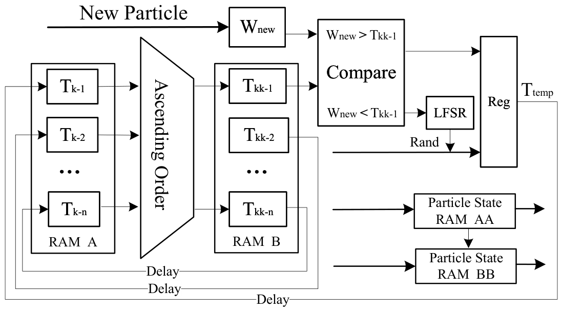
Figure 1 presents the architecture of the resampling module based on the OBMH sampling algorithm. The module utilizes two sets of dual-port Random Access Memories (RAMs) for data storage. Specifically, RAM A and RAM AA store the particle weights and their corresponding states before the update, while RAM B and RAM BB store the particle weights and their associated states after the update. The depth of each memory is denoted as n, which defines the size of the buffer region.

At system startup, the particle weights in RAM A are initialized. Subsequently, these weights are fed into an ascending sorting network, and the sorted results are written into RAM B. Concurrently, based on the address mapping information generated by the sorting network, the corresponding particle states stored in RAM AA are synchronously transferred to RAM BB, thereby ensuring consistency between the addresses of the sorted weights and their associated states.

After completing the weight calculation for the new online particle, the newly calculated weight is compared with the first weight stored in RAM B, which is the current minimum weight in the buffer. If the new particle weight is greater than this minimum weight, it directly replaces the first datum in RAM A. Otherwise, a uniformly distributed random number is generated using a Linear Feedback Shift Register (LFSR). Based on the generated random number, a weight is selected from RAM B to update the first datum in RAM A.

Meanwhile, the remaining weights in RAM B are updated into their corresponding positions in RAM A on a one-to-one basis according to their original addresses. After the completion of this update process, and prior to the arrival of the next new particle, all weights in RAM A are once again sorted through the ascending sorting network and stored back into RAM B. Simultaneously, the corresponding state data in RAM BB are updated, thus completing one full resampling cycle. The pseudo-code for the OBMH resampling algorithm is presented in Algorithm 1.

Algorithm 1 The proposed OBMH Resampling

1: Input: ${\{X_k^{\left(j\right)},w_k^{\left(j\right)}\}}_{j=1}^{L_{k-1}+J_k}$, n   2: Output: ${\{{\widehat{X}}_k^{\left(j\right)},{\widehat{w}}_k^{\left(j\right)}\}}_{j=1}^{L_k}$   3: Initialization: $B_k^{\left(1\right)}=X_k^{\left(1\right)}$, $B_k^{\left(2\right)}=X_k^{\left(2\right)},\dots ,B^{\left(n\right)}=X_k^{\left(n\right)}$;   4: $T_k^{\left(1\right)}=w_k^{\left(1\right)},T_k^{\left(2\right)}=w_k^{\left(2\right)},\dots ,T_k^{\left(n\right)}=w_k^{\left(n\right)}$   5: for $j=1,\dots ,L_{k-1}+J_k$ (can be executed in parallel pipeline) do   6:       $B_{kk}=Sort(B_k,T_k),T_{Kk}^{\left(1\right)}<T_{Kk}^{\left(2\right)}<\dots <T_{Kk}^{\left(n\right)}$   7:       if $w_k^{\left(j\right)}<T_{Kk}^{\left(1\right)}$ then   8:             generate a uniform random number $u\sim U\{1,2,\dots ,n\}$   9:             ${\widehat{X}}_k^{\left(j\right)}=B_{kk}^{\left(u\right)},{\widehat{w}}_k^{\left(j\right)}=T_{kk}^{\left(u\right)}$ 10:       else 11:             ${\widehat{X}}_k^{\left(j\right)}=x_k^{\left(j\right)},{\widehat{w}}_k^{\left(j\right)}=w_k^{\left(j\right)}$ 12:             update the buffer with new particle: $B_{Kk}^{\left(1\right)}=X_k^{\left(j\right)},T_{Kk}^{\left(1\right)}=w_k^{\left(j\right)}$ 13:             $B_k=B_{kk},T_k=T_{kk}$ 14:       end if 15:       $j=j+1$ 16: end for 17: ${\left\{{\widehat{X}}_k^{\left(j\right)}\right\}}_{j=1}^{L_k}\sim {\left\{{\widehat{X}}_k^{\left(j\right)}\right\}}_{j=1}^{L_{k-1}+J_k}$

By maintaining n buffer regions that store the states and weights of particles with relatively large weights in an ordered pattern, the OBMH algorithm achieves temporary caching of high-quality particles. This mechanism effectively prevents particles with significant weights in the current set from being immediately replaced by subsequent particles with even larger weights. Moreover, the algorithm allows the weight update step and the resampling step to be executed concurrently, substantially enhancing the real-time performance of the system in parallel devices.

5. Numerical Simulation and Analysis

Extensive numerical simulations are conducted to validate the effectiveness of the proposed algorithm. The simulations focus on evaluating adaptive particle generation, tracking performance, and computational efficiency.

5.1. Simulation Setup

A two-dimensional surveillance scene of size $35\times 35$ resolution units ($\Delta x=\Delta y=1$) is considered. The sensor parameters are: blur factor $\Sigma =0.7$, noise standard deviation $\sigma =1$. The total number of frames is $k=40$.

Target Dynamics: Each target’s state $X_k^t={[x_k^t,{\dot{x}}_k^t,y_k^t,{\dot{y}}_k^t,I_k^t]}^T$ evolves according to a nearly constant velocity model with random walk intensity:

$$X_{k+1}=F{X}_k+V_k,V_k\sim \mathcal{N}(0,Q),$$

(34)

$$F=\left[\begin{array}{ccccc}1& T& 0& 0& 0\\ 0& 1& 0& 0& 0\\ 0& 0& 1& T& 0\\ 0& 0& 0& 1& 0\\ 0& 0& 0& 0& 1\end{array}\right],Q=\left[\begin{array}{ccccc}{\displaystyle \frac{q_1}{3}}{T}^3& {\displaystyle \frac{q_1}{2}}{T}^2& 0& 0& 0\\ {\displaystyle \frac{q_1}{2}}{T}^2& q_{1}T& 0& 0& 0\\ 0& 0& {\displaystyle \frac{q_1}{3}}{T}^3& {\displaystyle \frac{q_1}{2}}{T}^2& 0\\ 0& 0& {\displaystyle \frac{q_1}{2}}{T}^2& q_{1}T& 0\\ 0& 0& 0& 0& q_{2}T\end{array}\right].$$

(35)

The parameter T represents the time interval period, and $T=1$ is set. In the matrix, $q_1=0.001$, which indicates the system noise affecting the target state; $q_2=0.01$, which represents the system noise affecting the target intensity amplitude.

Target Scenario: Three targets appear and disappear at different times, as detailed in Table 1. The intensity I determines the SNR, defined for a diffused target as:

$$SNR=10log{\left[{\displaystyle \frac{I\Delta x\Delta y}{2\pi {\Sigma }^2\sigma }}\right]}^2.$$

(36)

Intensities $I=15,9,7,5$ correspond to SNR values of approximately 13.75 dB, 9.32 dB, 7.13 dB, and 4.21 dB, respectively.

Table 1. Relevant Information of Targets in the Scenario.

Target	Initial State $[\mathit{x},\dot{\mathit{x}},\mathit{y},\dot{\mathit{y}},\mathit{I}]$	Appearance Frame	Disappearance Frame
1	[4, 0.35, 6, 0.8, I]	$k=2$	$k=24$
2	[5, 0.80, 6, 0.25, I]	$k=12$	$k=29$
3	[6, 0.65, 7, 0.6, I]	$k=30$	$k=40$

Table 1. Relevant Information of Targets in the Scenario.

Target	Initial State $[\mathit{x},\dot{\mathit{x}},\mathit{y},\dot{\mathit{y}},\mathit{I}]$	Appearance Frame	Disappearance Frame
1	[4, 0.35, 6, 0.8, I]	$k=2$	$k=24$
2	[5, 0.80, 6, 0.25, I]	$k=12$	$k=29$
3	[6, 0.65, 7, 0.6, I]	$k=30$	$k=40$

Filter Parameters: Survival probability $e_k=0.95$, birth probability ${\gamma }_k=0.2$, spawn probability $b_k=0$. Clutter intensity $K_k\left(z\right)$ is set based on the scene false alarm rate. The number of particles per frame $L_k$ is a variable parameter in experiments. $J_k$ is equal to $L_k$. The number of buffer particles is set to quarter $L_k$ by default in the proposed OBMH algorithm.

Performance Metrics: The statistical cardinality estimate, which reflects the estimated number of targets, is provided. Subsequently, the Optimal Sub-Pattern Assignment (OSPA) distance(with order $p=2$, cutoff $c=20$) is adopted as a measure of multi-objective deviation distance to evaluate the estimation error between the estimated state and the true state [43]. Results are averaged over 100 Monte Carlo runs.

5.2. Adaptive Particle Generation Performance

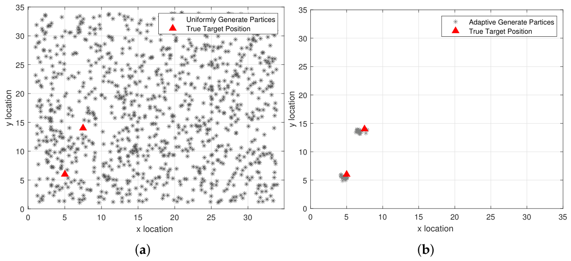
To demonstrate the advantages of the proposed adaptive particle generation method, Figure 2 presents two schematic diagrams depicting the distribution of newborn particles at the 12th frame of the simulation scenario. This frame includes two targets simultaneously: the surviving target (Target 1) and the newly emerged target (Target 2). The total number of newborn particles is set to 1024 in both cases. In the adaptive particle generation method, the number of candidate regions M is set to 10.

Figure 2a illustrates the conventional uniform particle generation approach, which distributes particles evenly across the entire monitoring area. When the total number of newborn particles is limited, each resolution unit contains only a sparse set of particles. Consequently, the effective number of particles available for approximating the target state becomes significantly reduced. Although increasing the total particle count could alleviate this issue, it would also lead to a substantial rise in computational burden, thereby compromising the real-time performance of the tracking algorithm.

In contrast, Figure 2b shows the result of the proposed adaptive particle generation strategy. When a new target initially appears, the newborn particles concentrate densely around the true target location. This concentrated distribution allows for a more accurate approximation of the target state posterior, which in turn promotes faster convergence of the particle filter.

5.3. Tracking Results Comparison

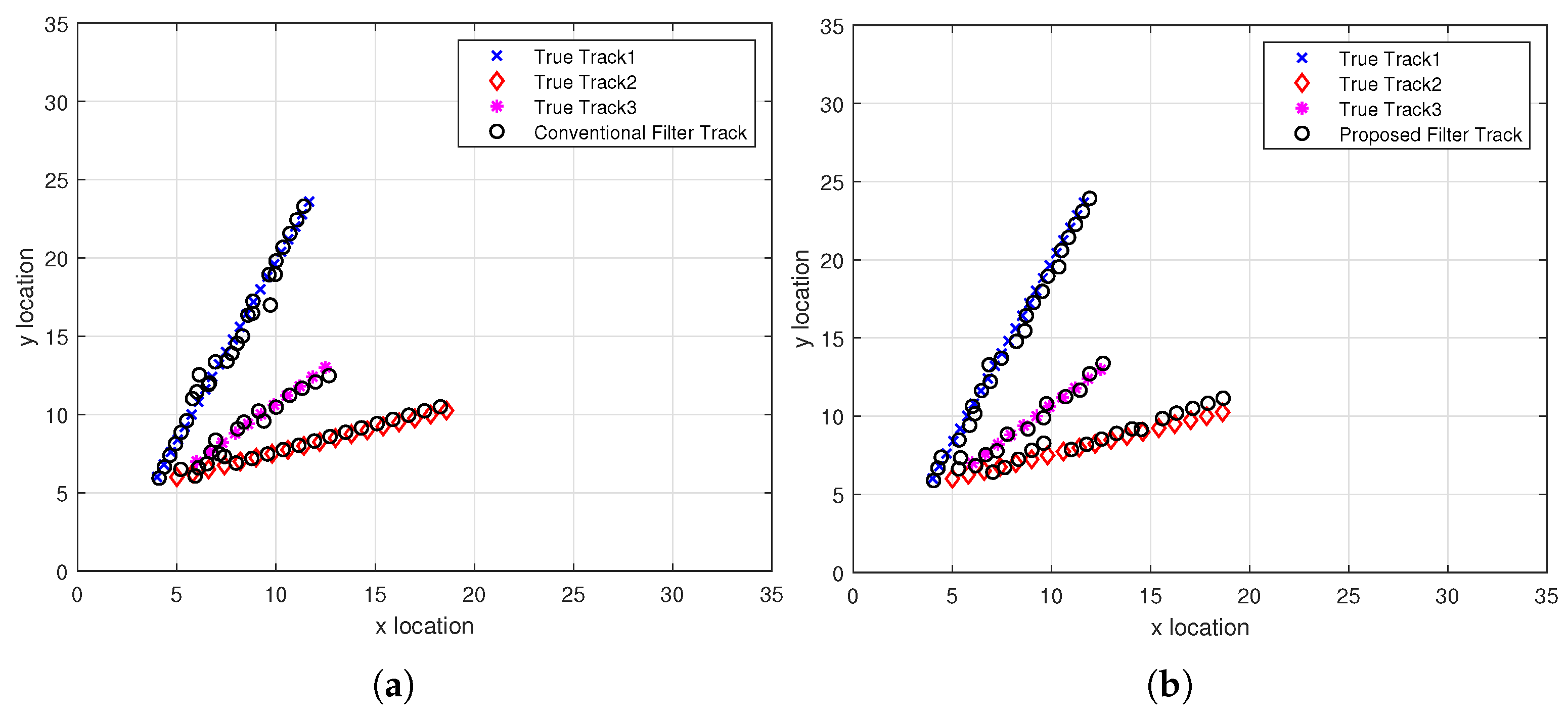
Under identical simulation conditions, Figure 3 presents a comparative analysis of the target state estimation results between the conventional method and the proposed method. The filtering results demonstrate that when targets emerge within the surveillance region, the estimated trajectories from both approaches largely align with the ground-truth target motions. Furthermore, both algorithms successfully accomplish multitarget tracking, generating continuous and consistent tracking trajectories throughout the observation period.

5.4. Algorithm Performance Evaluation

5.4.1. Performance Under Different Particle Counts

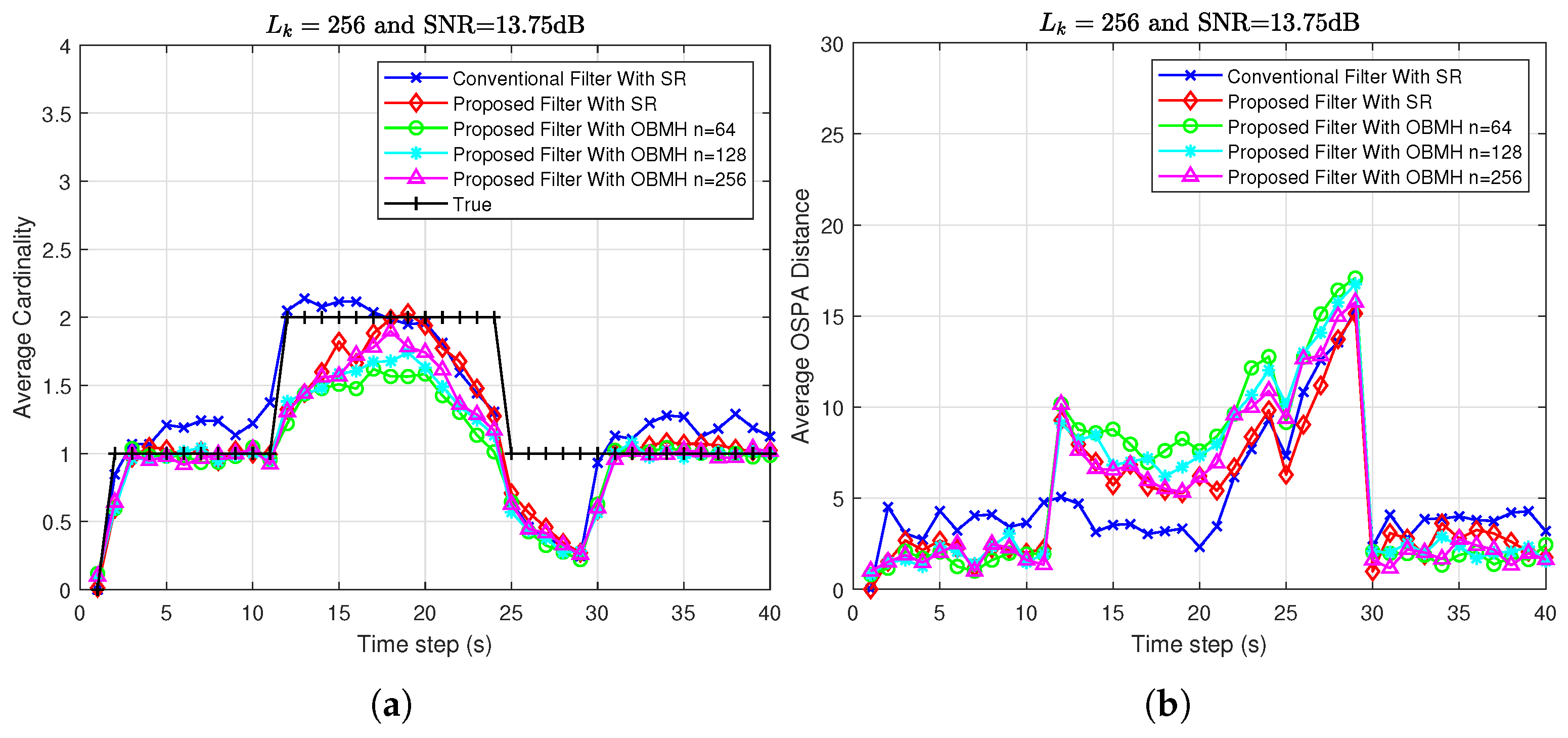
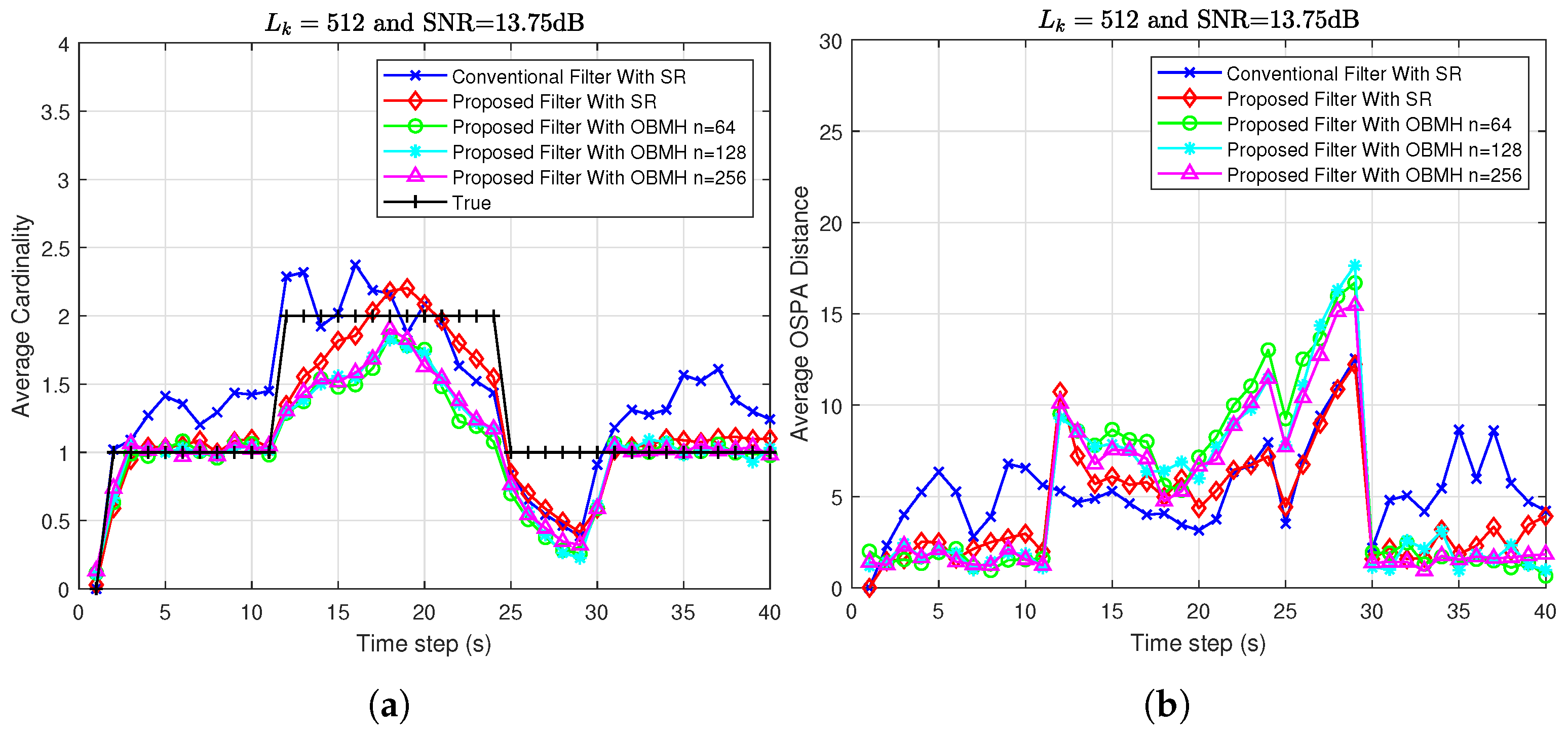
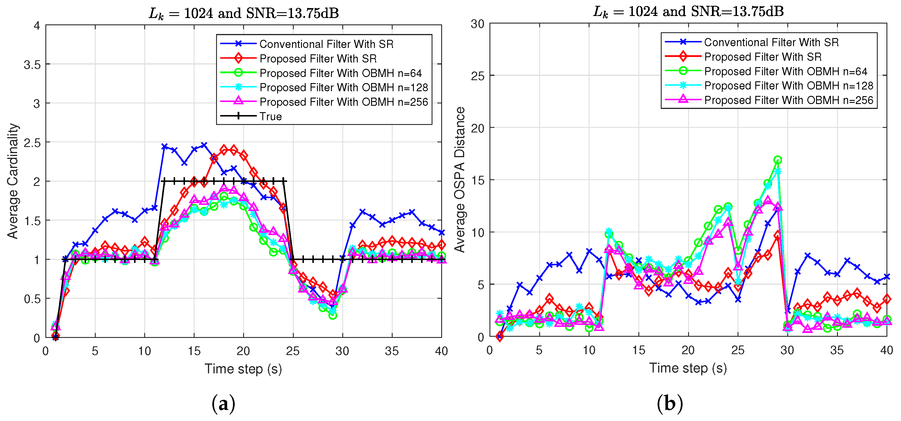
Under the condition of a constant SNR of 13.75 dB, the number of particles per frame is set to 256, 512, and 1024, respectively. The average cardinality estimates and OSPA distance curves are obtained through 100 Monte Carlo simulations. Under the same particle count configurations, the number of buffer particles in the OBMH resampling method is set to 64, 128, and 256, respectively. The simulation results are presented in Figure 4, Figure 5 and Figure 6.

As illustrated in the figures, the time intervals during which targets exist can be divided into three stages. The first stage spans from Frame 2 to Frame 11, during which only Target 1 exists, having been born in Frame 2. The second stage extends from Frame 12 to Frame 29, where both Target 1 and Target 2 are present, with Target 2 being born in Frame 12. The third stage covers Frames 30 to 40, during which only Target 3 exists, having been born in Frame 30.

As illustrated in Figure 4, when Target 1 appears in Frame 2, both algorithms are able to detect the target swiftly and provide accurate estimates of the target number. In scenarios where only one single target is present in the surveillance area, the proposed algorithm demonstrates superior cardinality estimation performance and achieves a smaller OSPA distance. When the second newborn target emerges in Frame 12, the conventional algorithm maintains accurate cardinality estimation. In contrast, both the proposed algorithm with SR resampling and the one with OBMH resampling require a two-frame delay to successfully track the newborn target. During this stage, the OSPA of the proposed algorithm increases rapidly; however, as the number of processed frames increases, the OSPA gradually converges. Overall, when two targets exist in the tracking scenario, the proposed algorithm with SR resampling achieves tracking performance comparable to that of the conventional algorithm. In comparison, the proposed algorithm with OBMH resampling has a slightly poorer tracking performance compared to the proposed algorithm with SR resampling. Furthermore, as the buffer size n increases in OBMH resampling, the filtering and tracking performance improves.

A comprehensive analysis of the simulation results presented in Figure 4, Figure 5 and Figure 6 reveals the following trends. As the number of particles per frame increases in the simulation scenario, and when only one single target is present in the surveillance area, the average cardinality estimation results of the conventional algorithm tend to increase. In contrast, the proposed algorithm with SR resampling and OBMH resampling maintains better average cardinality estimation results and achieves a smaller OSPA distance. During the second stage, where two targets are present in the surveillance area, the average cardinality estimation of both the conventional algorithm and the proposed algorithm have increased. Their average OSPA distances are approximately identical, indicating that the two algorithms achieve comparable tracking performance. Therefore, on the whole, the proposed algorithm is capable of retaining comparable tracking performance even when a relatively small number of particles is used.

5.4.2. Performance Under Different SNRs

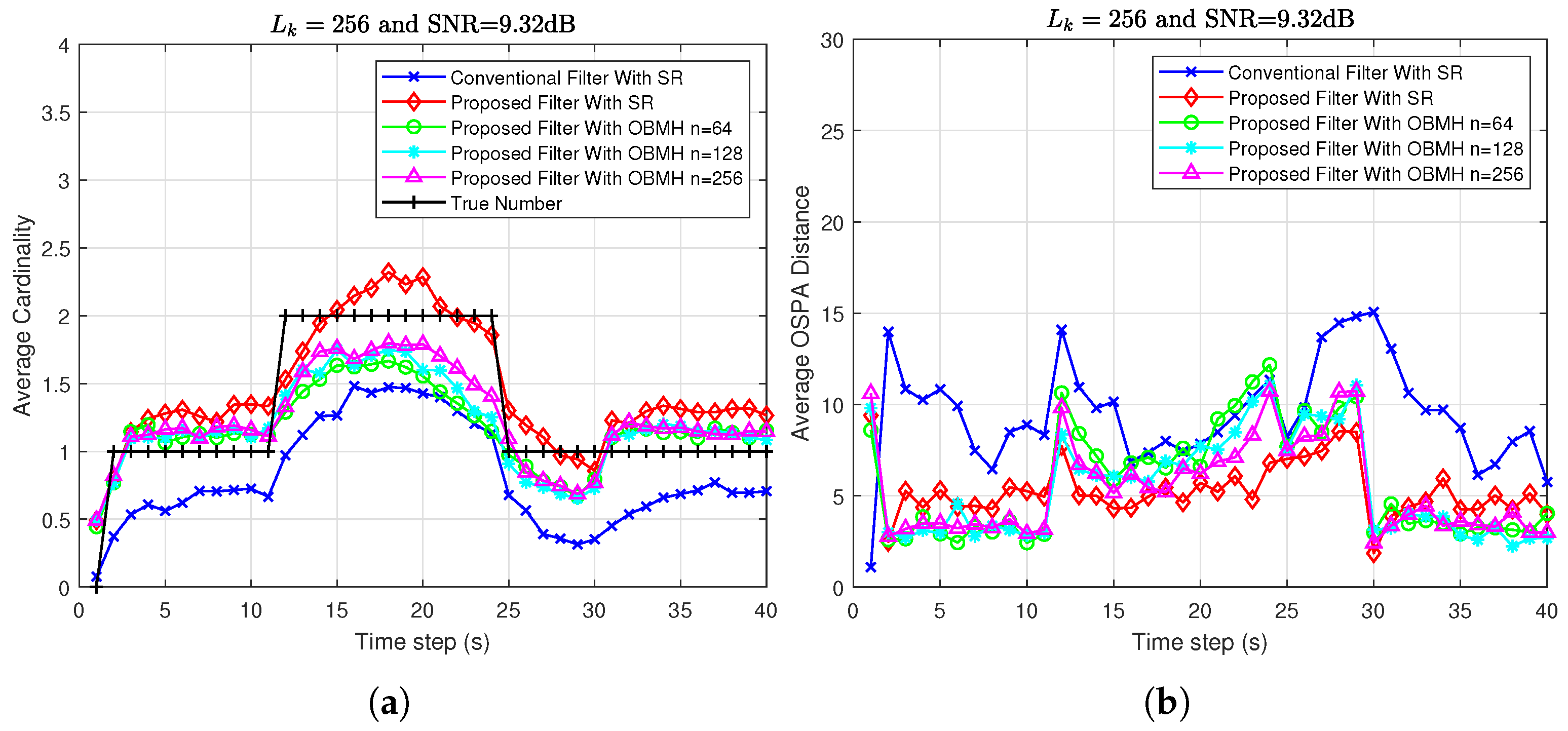
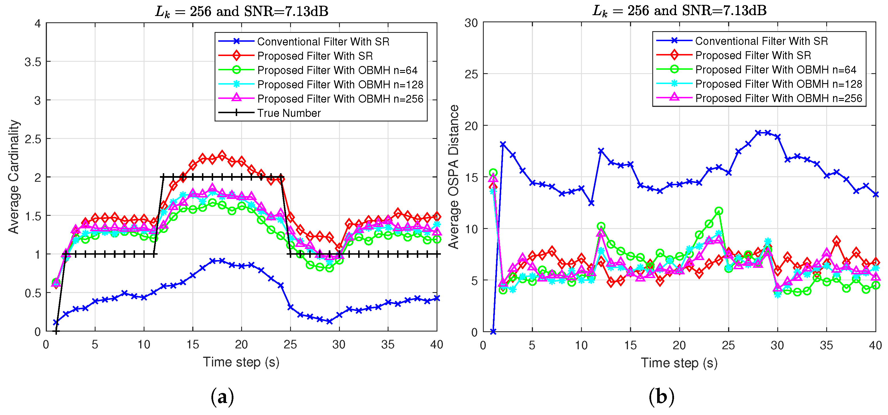
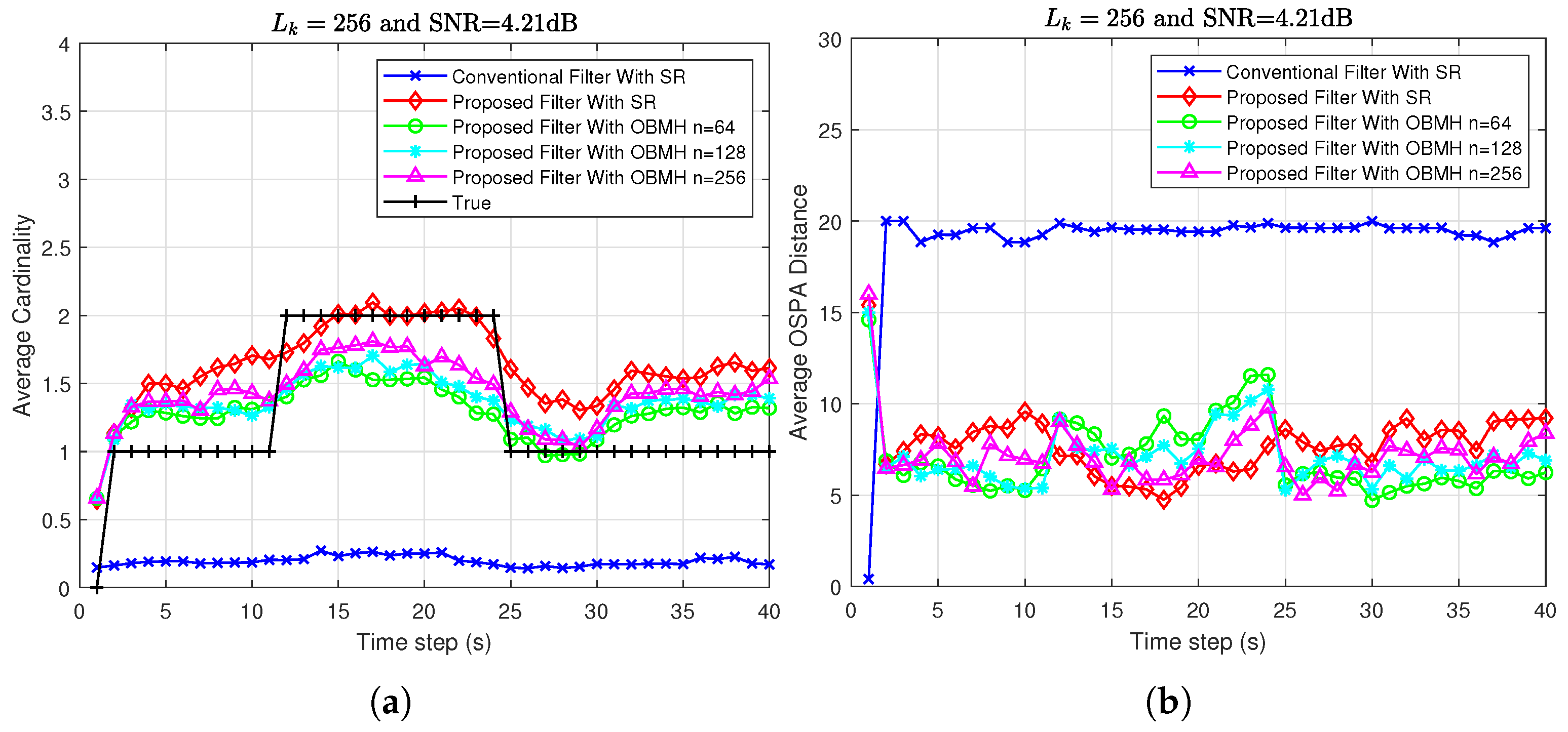
To evaluate the estimation performance of the proposed algorithm for weak and small targets, the number of particles per frame is set to 256. Under different SNR conditions, the target intensity is varied to 9, 7, and 5, corresponding to SNRs of 9.32 dB, 7.13 dB, and 4.21 dB, respectively. Using 100 Monte Carlo simulations, the performance of the proposed algorithm is compared against the conventional algorithms.

A comprehensive analysis of the simulation results presented in Figure 7, Figure 8 and Figure 9 reveals the following observations. Under a constant number of particles, as the target SNR continues to degrade, the performance of the conventional algorithm deteriorates sharply, with the average cardinality estimation results becoming notably underestimated. At an SNR of 4.21 dB, the conventional algorithm fails completely and is unable to detect any targets in the surveillance scene. However, as the SNR degrades, the average cardinality estimation results of the proposed algorithm gradually increase, but the estimated values fluctuate around the true value for most of the time. Even under the severe condition of SNR = 4.21 dB, the proposed algorithm is still able to maintain an accurate estimate of the target number in the majority of frames. Under low SNR conditions, the OSPA distance of the conventional algorithm increases substantially, whereas the proposed algorithm achieves a smaller OSPA distance, demonstrating a certain degree of tracking capability for weak targets. Overall, the proposed algorithm consistently outperforms the conventional algorithm.

5.4.3. Computational Time Consumption

In the experiments comparing algorithm performance across different particle numbers, the runtime for each trial is recorded. The average computational times for the proposed and conventional algorithms are summarized in

Table 2. Average Runtime Comparison.

Algorithm	256 Particles	512 Particles	1024 Particles
Conventional Filtered with SR	98.53 s	181.10 s	247.61 s
Proposed Filter with SR	12.48 s	51.56 s	67.49 s
Proposed Filter with OBMH n = 64	7.59 s	16.60 s	43.58 s
Proposed Filter with OBMH n = 128	8.19 s	19.67 s	52.98 s
Proposed Filter with OBMH n = 256	10.34 s	30.62 s	59.19 s

. Owing to hardware constraints, all simulations are performed under identical experimental conditions using MATLAB R2021a (The MathWorks, Inc., Natick, MA, USA) on a standard desktop PC equipped with a 3.2 GHz CPU and 64 GB of RAM.

As clearly shown in the table, the proposed algorithm achieves significantly higher execution efficiency than the conventional algorithm, as evidenced by its considerably shorter average runtime per experiment. This improvement in computational speed is attributed to two key enhancements that collectively reduce computational complexity: the generation of effective newborn particles and the simplification of weight calculation. These enhancements together minimize redundant weight-related computations. Moreover, deploying the algorithm on a parallel hardware platform allows weight calculation and OMBH-based resampling to be performed in parallel, thereby further enhancing its real-time performance.

6. Conclusions

This paper presented a rapid implementation of a non-sequential particle PHD-TBD. Simulation results demonstrated that the proposed algorithm achieves comparable or superior tracking accuracy to the conventional algorithm while requiring significantly fewer particles. It exhibits strong robustness in low-SNR scenarios where the conventional filter fails. Most notably, it reduces computational time in tested scenarios, making it highly suitable for real-time applications.

Nevertheless, the proposed algorithm still has notable limitations. The algorithm’s performance has only been validated under a nearly constant velocity motion model, and the diversity of target motion is not considered, such as highly maneuvering targets or crossing target trajectories. To address these shortcomings, future research will introduce maneuvering target motion models and target trajectory crossing scenarios. In particular, we will explore optimization strategies to overcome potential failures when the target undergoes rapid turns, as well as the partial merging of particle clouds from different targets during trajectory crossing that may cause temporary track ambiguity. The goal is to maintain competitive tracking performance while pursuing fast implementation, thereby improving the robustness and adaptability of the algorithm.

Meanwhile, although the proposed algorithm significantly improves the computational efficiency while maintaining the tracking accuracy, its current implementation is designed primarily for the two-dimensional image observation model and has not been fully extended to DOA tracking with sparse or coprime array setups. Existing research has applied the particle PHD-TBD framework to DOA tracking. Building upon this foundation, integrating our data-driven adaptive particle generation and parallel resampling schemes can diminish invalid particles, and enable parallel execution of weight computation and resampling. Such improvements are expected to further reduce the computational cost, enhance the real-time performance of DOA estimation and multi-target tracking, and provide a feasible technical path for engineering deployment on resource-constrained platforms.

For future work, we will focus on the engineering deployment of the proposed algorithm on parallel hardware platforms. The core computational procedures of our approach, namely particle generation, particle weight calculation, and OBMH resampling, possess strong inherent data parallelism. FPGAs are highly suitable for deep pipeline optimization, where multiple particles can be processed simultaneously in each clock cycle. Specifically, the buffer and sorting networks required for OBMH resampling can be mapped to on-chip block RAMs and comparator arrays to further lower processing latency. For GPU implementations, each particle can be assigned to an independent CUDA thread, which supports batched particle generation and weight updates and delivers parallel acceleration for batch computation and sorting. Thanks to the strong parallel computation architectures, the proposed method satisfies real-time latency demands of operational radar systems and holds great promise for real-world deployment.

In summary, while the proposed algorithm achieves a certain degree of improvement in real-time performance, overcoming its current limitations is essential to enhancing its practicality and robustness. Future efforts will be directed toward algorithm optimization and deployment on parallel hardware platforms, thereby rendering it more applicable to real-world scenarios in complex tracking scenarios.

References

1. Boers, Y.; Driessen, J.; Verschure, F.; Heemels, W.; Juloski, A. A Multi Target Track Before Detect Application. In Proceedings of the IEEE Conference on Computer Vision and Pattern Recognition Workshop, Madison, WI, USA; IEEE: Piscataway, NJ, USA, 2003; pp. 104–110. [Google Scholar]
2. Sang, H.; Zheng, R.; Cheng, H.; Meng, X.; Li, L.; Qi, J. A Review of Point Target and Extended Target Tracking Algorithms. In Proceedings of the 2024 3rd International Conference on Image Processing and Media Computing (ICIPMC), Hefei, China, 17–19 May 2024; pp. 335–346. [Google Scholar]
3. Mahler, R. Multitarget Bayes Filtering via First-Order Multitarget Moments. IEEE Trans. Aerosp. Electron. Syst. 2003, 39, 1152–1178. [Google Scholar] [CrossRef]
4. Vo, B.; Ma, W. A Closed-Form Solution for the Probability Hypothesis Density Filter. In Proceedings of the 8th International Conference on Information Fusion, Philadelphia, PA, USA, 27 June–1 July 2005; pp. 856–863. [Google Scholar]
5. Mahler, R. PHD Filters of Higher Order in Target Number. IEEE Trans. Aerosp. Electron. Syst. 2007, 43, 1523–1543. [Google Scholar] [CrossRef]
6. Vo, B.N.; Ma, W.K. The Gaussian Mixture Probability Hypothesis Density Filter. IEEE Trans. Signal Process. 2006, 54, 4091–4104. [Google Scholar] [CrossRef]
7. Vo, B.; Singh, S.; Doucet, A. Sequential Monte Carlo Methods for Multitarget Filtering with Random Finite Sets. IEEE Trans. Aerosp. Electron. Syst. 2005, 41, 1224–1245. [Google Scholar] [CrossRef]
8. Zeng, Y.; Wang, J.; Wei, S.; Zhang, C.; Zhou, X.; Lin, Y. Gaussian Mixture Probability Hypothesis Density Filter for Heterogeneous Multi-Sensor Registration. Mathematics 2024, 12, 886. [Google Scholar] [CrossRef]
9. Liu, J.; Wang, C.; Wang, W.; Li, Z. Particle Probability Hypothesis Density Filter Based on Pairwise Markov Chains. Algorithms 2019, 12, 31. [Google Scholar] [CrossRef]
10. Bolić, M.; Djurić, P.; Hong, S. New Resampling Algorithms for Particle Filters. In Proceedings of the IEEE International Conference on Acoustics, Speech and Signal Processing; IEEE: Piscataway, NJ, USA, 2003; pp. 589–592. [Google Scholar]
11. Li, T.; Bolić, M.; Djurić, P.M. Resampling Methods for Particle Filtering: Classification, Implementation, and Strategies. IEEE Signal Process. Mag. 2015, 32, 70–86. [Google Scholar] [CrossRef]
12. Sankaranarayanan, A.C.; Srivastava, A.; Chellappa, R. Algorithmic and Architectural Optimizations for Computationally Efficient Particle Filtering. IEEE Trans. Image Process. 2008, 17, 737–748. [Google Scholar] [CrossRef] [PubMed]
13. Zheng, Y.; Shi, Z.; Lu, R.; Hong, S.; Shen, X. An Efficient Data-Driven Particle PHD Filter for Multitarget Tracking. IEEE Trans. Ind. Inform. 2013, 9, 2318–2326. [Google Scholar] [CrossRef]
14. Li, T.; Sun, S.; Bolić, M.; Corchado, J.M. Algorithm Design for Parallel Implementation of the SMC-PHD Filter. Signal Process. 2016, 119, 115–127. [Google Scholar] [CrossRef]
15. Yang, C.; Shi, Z.; Zhang, J.J.; Gu, Y.; Qin, Z. Optimization of Particle CBMeMBer Filters for Hardware Implementation. IEEE Trans. Veh. Technol. 2018, 67, 9027–9031. [Google Scholar] [CrossRef]
16. Zhang, H.; Tao, H.; Shen, X.; Zhang, L.; Ruan, Z. Improved Residual Cumulative Resampling PF-PHD Filter Based on Stratified Rough Sorting. In Proceedings of the 8th International Conference on Image, Vision and Computing (ICIVC), Dalian, China, 27–29 July 2023; pp. 874–879. [Google Scholar]
17. Wood, T. Detecting and Tracking Multiple Stealthy Targets: Comparison of PHD Filter and Track-Before-Detect Approaches. In Proceedings of the 2nd IMA Conference on Mathematics in Defence, Swindon, UK, 20 October 2011; pp. 1–6. [Google Scholar]
18. Punithakumar, K.; Kirubarajan, T.; Sinha, A. A Sequential Monte Carlo Probability Hypothesis Density Algorithm for Multitarget Track-Before-Detect. In Proceedings of the SPIE Signal and Data Processing of Small Targets, San Diego, CA, USA, 2–4 August 2005; pp. 591–598. [Google Scholar]
19. Zhan, R.; Zhang, J. Improved Multitarget Track-Before-Detect for Image Measurements. In Proceedings of the 2012 IEEE 11th International Conference on Signal Processing, Beijing, China; IEEE: Piscataway, NJ, USA, 2012; pp. 2183–2187. [Google Scholar]
20. Lin, Z.P.; Zhou, Y.Y.; An, W. Improved Multitarget Track-Before-Detect Using Probability Hypothesis Density Filter. J. Infrared Millim. Waves 2012, 31, 475–480. [Google Scholar] [CrossRef]
21. Zhan, R.; Liu, S.; Ou, J.; Zhang, J. Improved Multitarget Track-Before-Detect Algorithm Using the Sequential Monte Carlo Probability Hypothesis Density Filter. J. Electron. Inf. Technol. 2014, 36, 2593–2599. [Google Scholar]
22. Zhan, R.; Gao, Y.; Hu, J.; Zhang, J. SMC-PHD Based Multi-Target Track-Before-Detect with Nonstandard Point Observations Model. J. Cent. South Univ. 2015, 22, 232–240. [Google Scholar] [CrossRef]
23. Luo, X.; Yang, C.; Chen, R.; Shi, Z. Improved SMC-PHD Filter for Multi-Target Track-Before-Detect. In Proceedings of the 84th IEEE Vehicular Technology Conference; IEEE: Piscataway, NJ, USA, 2016; pp. 1–6. [Google Scholar]
24. Shi, Z.; Zhang, Y. Derivation of PHD-TBD filter and comments on ‘joint detection and estimation of multiple objects from image observations’. In Applications of Digital Image Processing XXXIX; San Diego, CA, USA, 29 August–1 September 2016; Proc. SPIE 9971; SPIE: Bellingham, WA, USA, 2016; p. 99713A. [Google Scholar]
25. Zhu, R.; Long, Y.; Sha, Z.; An, W. Multitarget Track-Before-Detect from Image Observations Based on Multi-Object Particle PHD Filter. In Proceedings of the 2017 Progress in Electromagnetics Research Symposium-Spring (PIERS), St. Petersburg, Russia, 22–25 May 2017; pp. 3062–3066. [Google Scholar]
26. Long, Y.; Xu, H.; An, W.; Liu, L. Track-Before-Detect for Infrared Maneuvering Dim Multi-Target via MM-PHD. Chin. J. Aeronaut. 2012, 25, 252–261. [Google Scholar] [CrossRef]
27. Zhang, Y.; Long, Y.; Liu, K. Track-Before-Detect Algorithm for Maneuvering Infrared Weak Multiple Targets via Particle Filter. Chin. Opt. Lett. 2014, 12, 101101. [Google Scholar] [CrossRef][Green Version]
28. Bao, Z.; Jiang, Q.; Liu, F. A PHD Based Particle Filter for Detecting and Tracking Multiple Weak Targets. IEEE Access 2019, 7, 145843–145850. [Google Scholar] [CrossRef]
29. Lin, Z.; Zhou, Y.; An, W. Track-Before-Detect Algorithm Based on Probability Hypothesis Density Smoother. Acta Opt. Sin. 2012, 32, 1201003. [Google Scholar] [CrossRef]
30. Zhu, H.; Huang, Y.; Jiang, B.; Guan, J. A Gaussian Mixture Probability Hypothesis Density Smoothing Algorithm for Multi-Target Track-Before-Detect. In Proceedings of the 2016 IEEE International Conference on Signal and Image Processing; IEEE: Piscataway, NJ, USA, 2016; pp. 1562–1565. [Google Scholar]
31. Ikoma, N. Multiple Pedestrians Tracking with Composite Sensor of Laser Range Finder and Omni-Directional Camera by SMC Implementation of PHD Filter. In Proceedings of the 6th International Conference on Soft Computing and Intelligent Systems, and the 13th International Symposium on Advanced Intelligence Systems, Kobe, Japan, 20–24 November 2012; pp. 705–710. [Google Scholar]
32. Saucan, A.; Chonavel, T.; Sintes, C.; Caillec, J.L. Marked Poisson Point Process Probe PHD Filter for DOA Tracking. In Proceedings of the 2015 23rd European Signal Processing Conference (EUSIPCO), Nice, France, 31 August–4 September 2015; pp. 2621–2625. [Google Scholar]
33. Saucan, A.; Chonavel, T.; Sintes, C.; Caillec, J.L. Track Before Detect DOA Tracking of Extended Targets with Marked Poisson Point Processes. In Proceedings of the 2015 18th International Conference on Information Fusion (Fusion), Washington, DC, USA, 6–9 July 2015; pp. 754–760. [Google Scholar]
34. Tong, H.; Zhang, H.; Meng, H.; Wang, X. Multitarget Tracking Before Detection via Probability Hypothesis Density Filter. In Proceedings of the International Conference on Electrical and Control Engineering (ICECE), Wuhan, China, 25–27 June 2010; pp. 1332–1335. [Google Scholar]
35. Tong, H.; Zhang, H.; Meng, H.; Wang, X. A Shrinkage Probability Hypothesis Density Filter for Multitarget Tracking. EURASIP J. Adv. Signal Process. 2011, 2011, 116. [Google Scholar] [CrossRef]
36. Habtemariam, B.K.; Tharmarasa, R.; Kirubarajan, T. PHD Filter Based Track-Before-Detect for MIMO Radars. Signal Process. 2012, 92, 667–678. [Google Scholar] [CrossRef]
37. Pei, J.; Huang, Y.; Dong, Y.; Chen, B. Multitarget Track-Before-Detect Based on Auxiliary Parallel Partition Particle PHD Filter. In Proceedings of the 2018 International Conference on Radar (RADAR), Brisbane, QLD, Australia, 27–31 August 2018; pp. 1–6. [Google Scholar]
38. Mao, H.; Zhang, B.; Yang, J.; Long, X.; Peng, C.; Yi, W. Labeled Probability Hypothesis Density Filtering for Track-Before-Detect Strategy. In Proceedings of the 2023 26th International Conference on Information Fusion (FUSION), Charleston, SC, USA, 27–30 June 2023; pp. 1–8. [Google Scholar]
39. Mao, H.; Peng, C.; Liu, Y.; Tang, J.; Peng, H.; Yi, W. Poisson Conjugate Prior for PHD Filtering Based Track-Before-Detect Strategies in Radar Systems. In Proceedings of the 2023 IEEE Radar Conference (RadarConf23), San Antonio, TX, USA; IEEE: Piscataway, NJ, USA, 2023; pp. 1–6. [Google Scholar]
40. Chen, Z.; Peng, X.; Yang, J.; Zhong, Z.; Song, Q.; Zhang, Y. A Hybrid Integration Method Based on SMC-PHD-TBD for Multiple High-Speed and Highly Maneuverable Targets in Ubiquitous Radar. Remote Sens. 2024, 16, 14. [Google Scholar]
41. Cheng, L.; Sengupta, A.; Cao, S. Deep Learning-Based Robust Multi-Object Tracking via Fusion of mmWave Radar and Camera Sensors. IEEE Trans. Intell. Transp. Syst. 2024, 25, 17218–17233. [Google Scholar] [CrossRef]
42. Haensel, L.; Bertram, T. Robust Multiobject Tracking Using MmWave Radar-Event-Camera Sensor Fusion. In Proceedings of the 11th International Conference on Control, Decision and Information Technologies (CoDIT), Split, Croatia, 15–18 July 2025; pp. 2656–2659. [Google Scholar]
43. Schuhmacher, D.; Vo, B.T.; Vo, B.N. A Consistent Metric for Performance Evaluation of Multi-Object Filters. IEEE Trans. Signal Process. 2008, 56, 3447–3457. [Google Scholar] [CrossRef]
Figure 1. The architecture of the proposed OBMH algorithm.
Electronics 15 02782 g001
Figure 2. Schematic Diagram of Particle Generation: (a) Uniform Particle Generation. (b) Adaptive Particle Generation.
Electronics 15 02782 g002
Figure 3. Schematic Diagram of Filtering State Estimation: (a) Estimation by the Conventional Algorithm. (b) Estimation by the Proposed Algorithm.
Electronics 15 02782 g003
Figure 4. Performance Comparison of Filtering with Different Parameter Settings (Particles per frame: 256): (a) Average Cardinality Estimation. (b) Average OSPA Distance.
Electronics 15 02782 g004
Figure 5. Performance Comparison of Filtering with Different Parameter Settings (Particles per frame: 512): (a) Average Cardinality Estimation. (b) Average OSPA Distance.
Electronics 15 02782 g005
Figure 6. Performance Comparison of Filtering with Different Parameter Settings (Particles per frame: 1024): (a) Average Cardinality Estimation. (b) Average OSPA Distance.
Electronics 15 02782 g006
Figure 7. Performance Comparison of Filtering with Different Parameter Settings (SNR = 9.32 dB): (a) Average Cardinality Estimation. (b) Average OSPA Distance.
Electronics 15 02782 g007
Figure 8. Performance Comparison of Filtering with Different Parameter Settings (SNR = 7.13 dB): (a) Average Cardinality Estimation. (b) Average OSPA Distance.
Electronics 15 02782 g008
Figure 9. Performance Comparison of Filtering with Different Parameter Settings (SNR = 4.21 dB): (a) Average Cardinality Estimation. (b) Average OSPA Distance.
Electronics 15 02782 g009