An Anti-Swept-Frequency-Jamming Communication Method Based on Proximal Policy Optimization for Nonlinear Scenarios

Abstract

With the advancement in electronic attack technologies, intelligent jamming poses a significant challenge to the reliable transmission of wireless communications. Traditional anti-jamming methods often fail to adapt to dynamic nonlinear jamming environments. This paper addresses nonlinear swept-frequency jamming by modeling anti-jamming communication as a sequential decision-making problem and proposes an intelligent anti-jamming method based on proximal policy optimization (PPO) to optimize dynamic channel selection. Firstly, the channel selection problem is formalized as a Markov decision process (MDP), where a state space integrating jamming patterns and communication status is designed, the channel set is defined as the action space, and a multi-objective reward function trades off jamming avoidance against switching overhead. A dual-network architecture comprising a policy network and a value network is constructed, and the PPO algorithm is employed for policy updates, where a clipping mechanism is used to enhance training stability. The system optimizes the anti-jamming strategy online through a closed-loop process of “sensing–decision–learning–communication”. Simulation results demonstrate that compared to conventional methods, the proposed method significantly improves key performance indicators such as packet success rate and throughput. It can rapidly track changes in jamming, exhibiting excellent real-time performance and environmental robustness, and thus provides an effective solution for reliable communication in dynamic jamming environments.

1. Introduction

Over the past two decades, wireless communications have been widely adopted across various economic and social sectors. However, since wireless communications rely on electromagnetic waves to propagate information, the reliability and effectiveness of transmission are highly vulnerable to severe intentional or unintentional interference [1]. Therefore, anti-jamming is a critical issue that must be addressed in wireless communications.

Conventional spread spectrum (SS) techniques are classic anti-jamming methods and remain extensively deployed in various wireless communication systems [2]. However, because conventional SS waveforms and strategies are fixed, they can only defend against specific types of jamming and are ill-suited to highly dynamic threats such as swept-frequency jamming [3]. In recent years, with the rapid development of artificial intelligence technologies such as machine learning, intelligent anti-jamming methods have been extensively investigated [4,5]. Ref. [6] addressed the slow convergence and high resource consumption of reinforcement learning-based anti-jamming algorithms in unknown dynamic jamming environments by proposing a fast anti-jamming method assisted by intra-domain knowledge reuse based on bisimulation relations. The method improved the convergence speed of the anti-jamming strategy, the normalized throughput, and the system’s agility and memory capability in dynamic jamming environments. Ref. [7] tackled the challenges of online learning, high computational complexity, and ensuring single-user optimality in spectrum anti-jamming for multi-IoT-device uplink transmissions by proposing a sequential multi-agent reinforcement learning method based on Gaussian kernel value function approximation. This method enhanced the average normalized throughput and enabled each user to converge independently to the optimal frequency-domain configuration in dynamic jamming environments. Ref. [8] focused on high computational cost and slow online learning of deep reinforcement learning for hardware-constrained UAVs in dynamic jamming environments by proposing a lightweight reinforcement learning method based on state clustering networks and tabular Q-learning. The proposed method improved the system’s convergence speed, adaptive capability, and resource efficiency in complex dynamic jamming environments while achieving an anti-jamming performance comparable to that of deep reinforcement learning. Ref. [9] addressed the anti-jamming decision problem in distributed multi-user dynamic spectrum access with limited channel resources, where users could only acquire local information and lacked reliable control links. A cooperative anti-jamming method based on intelligent frequency reuse and hybrid-reward multi-agent deep reinforcement learning was proposed, which improved the normalized throughput and reduced communication delay in complex dynamic jamming environments, and enabled synchronous learning of frequency reuse and anti-jamming strategies among users. Ref. [10] addressed throughput degradation and dynamic environment adaptation caused by jamming attacks in wireless networks by proposing an intelligent anti-jamming method based on deep reinforcement learning and transfer learning. By employing recurrent neural networks to reduce the parameter count, introducing an integrated feature extractor to measure domain discrepancy, and designing an interpretable feature correlation analysis mechanism, this method significantly accelerated training and improved environmental adaptability of the anti-jamming strategy, thereby enhancing network throughput and anti-jamming performance.

In complex and dynamic electromagnetic environments, swept-frequency jamming has become one of the most threatening jamming techniques against wireless communication, radar, and navigation systems due to its high efficiency, flexibility, and strong adaptability [11]. By periodically sweeping the carrier frequency of the jamming signal across a specific frequency band according to a certain pattern, it can effectively disrupt fixed-frequency communication systems and conventional frequency-hopping systems that rely on narrowband filtering. With the increasing intelligence of jammers, swept-frequency jamming is evolving from an initial stage characterized by fixed patterns and single parameters to a complex, advanced stage featuring nonlinearity, variable sweeping rates, and multi-mode coordination [12]. Correspondingly, anti-swept-frequency-jamming methods must evolve from rule-based approaches to AI-based solutions [13].

The essence of swept-frequency jamming lies in the time-varying nature of its carrier frequency. Based on its frequency variation pattern, sweeping rate, and structural complexity, swept-frequency jamming can be categorized as follows:

• Linear swept-frequency jamming: The frequency of the jamming signal changes linearly with time (either increasing or decreasing). This is the most basic form—mathematically simple and easy to generate—but its regularity also makes it relatively easy to predict and track. Its primary function is to sweep over a wide frequency band and suppress communication across multiple channels within that band.
• Nonlinear swept-frequency jamming: The frequency variation of the jamming signal follows a nonlinear function, such as a sinusoidal, exponential, or random pattern. This jamming mode is complex and difficult to capture with simple models. It significantly complicates parameter estimation and prediction for wireless communication systems, and can effectively counter traditional anti-jamming algorithms based on fixed models.

In recent years, artificial intelligence technologies centered on machine learning have developed rapidly, offering new approaches for achieving autonomous, dynamic, and forward-looking anti-jamming methods, particularly against nonlinear swept-frequency jamming. As a core methodology in machine learning, deep reinforcement learning (DRL) provides a powerful means to address the high-dimensional, dynamic, and highly stochastic nature of anti-jamming problems in wireless communications [14]. Among the DRL algorithms, PPO stands out for its excellent stability, high sample efficiency, and relatively simple implementation, and has become one of the most prominent DRL algorithms in the wireless communication domain. PPO introduces the trust region concept and a clipping mechanism, effectively balancing the exploration–exploitation trade-off as well as learning speed and stability. This makes it particularly suitable for online learning and optimization scenarios in wireless communication systems that have stringent requirements for real-time performance, reliability, and policy smoothness.

However, existing research has mostly focused on relatively static optimization scenarios or those with known models, or has treated jamming merely as background noise. Although PPO performs excellently in general resource management problems [15], research specifically targeting PPO-based algorithms in highly dynamic, intelligent, and strongly adversarial jamming environments—especially nonlinear swept-frequency jamming—remains insufficient. Most existing studies do not fully consider strongly adversarial scenarios in which jammers possess cognitive capabilities [16] and can learn to counter the communication system’s anti-jamming strategies. In such scenarios, the non-stationarity of the environment increases sharply, posing challenges to convergence stability, policy robustness, and the adaptation speed of learning algorithms. Therefore, investigating PPO-based methods capable of rapidly and stably learning optimal anti-jamming strategies in such strongly adversarial environments, and deeply integrating them with specific physical-layer communication processes (such as dynamic channel switching), holds significant theoretical value and practical significance. This paper addresses the severe challenge of nonlinear swept-frequency jamming with dynamically time-varying sweeping rate and direction by proposing and implementing a complete intelligent anti-jamming communication solution. The main contributions of this paper are as follows:

• Different from existing PPO-based anti-jamming works that address linear or fixed-rate swept-frequency jamming, this paper specifically targets nonlinear swept-frequency jamming scenarios where the frequency variation follows a nonlinear function and the sweeping rate and direction vary dynamically over time.
• By formalizing the anti-jamming channel selection problem as a sequential decision-making problem, a communication adversarial MDP model is constructed, and a composite state space representation method integrating historical time–frequency trajectories is proposed. This enables the agent to learn the motion patterns of the jamming signal and achieve proactive channel selection.

2. System Model and Problem Formulation

2.1. System Model

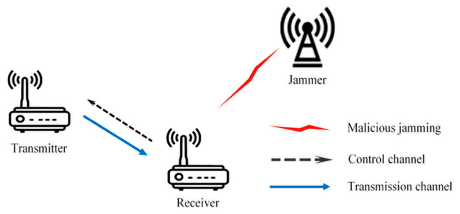
This paper considers an adversarial scenario involving a wireless communication system and a malicious jammer, as illustrated in Figure 1. The wireless communication system comprises a transmitter and a receiver; the data transmission between them is subject to malicious jamming by the jammer. The jammer is capable of transmitting a swept-frequency jamming signal, and its jamming signal can effectively cover the receiver.

To facilitate theoretical analysis and algorithm design, the following assumptions are made for the system model:

• The frequency band is divided into $N$ non-overlapping channels, denoted by $F=\{f_1 ,f_2 ,\dots ,f_{\mathrm{N}} \}$, each with a bandwidth of $B_c$. The system operates in a time-slotted manner, with each slot of duration $T_s$ serving as the minimum time unit for continuous signal transmission. In each time slot, the transmitter selects one channel for data transmission, with fixed transmission power $P_c$ and data rate $R_c$.
• The jammer employs a nonlinear swept-frequency jamming strategy, in which the center frequency of the jamming signal varies dynamically over time. The frequency-sweeping trajectory can be modeled as a continuous-time process, and the instantaneous jamming channel, denoted by $f_J (t)$, can be expressed as:

$$f_J (t)=f_0+{\int }_0^{\mathrm{t}}v(\tau )\mathrm{d}\tau ,$$

(1)

where $f_0$ is the initial jamming frequency, and $v(\tau )$ is the time-varying sweeping rate, whose magnitude and direction can both vary randomly. The minimum duration of the jamming signal is one time slot $T_s$, and the jamming power $P_J$ remains constant. The jammer can adaptively adjust its sweeping pattern based on previously observed communication signal characteristics, thereby exhibiting a degree of intelligence.

3.

The system makes decisions at each discrete time slot. At the beginning of time slot $t$, the receiver senses the current jamming state. Based on the sensing information, the intelligent anti-jamming algorithm generates a channel selection action $a_t\in F$ in real-time. The transmitter and receiver then synchronously switch to the selected channel for data transmission during that time slot. At the end of the time slot, the system calculates a reward $r_t$ based on the communication outcome and updates the network parameters.

4.

Communication success depends on the frequency distance between the selected communication channel and the jamming channel. The normalized distance between them is defined as:

$$d_t=\frac{|f_c(t)-f_J(t)|}{N-1},$$

(2)

where $f_c(t)$ and $f_J(t)$ denote the indices of the communication channel and the jamming channel at time slot $t$, respectively. When $d_t =0$, the two channels fully overlap, causing severe communication degradation. The received signal quality is measured by the signal-to-jamming-plus-noise ratio (SJNR):

$${\mathrm{SJNR}}_t ={\displaystyle \frac{P_c\cdot h_t}{P_J \cdot \mathrm{g}(d_t)+{\sigma }^2}},$$

(3)

where $\mathrm{g}(d_t)$ is the distance-dependent jamming attenuation function, ${\sigma }^2$ is the noise power, and $h_t$ is the channel fading coefficient. In this paper, since a certain line-of-sight (LoS) component generally exists between the transmitter and the receiver, we introduce Rician fading. $h_t$ follows a Rician distribution. The probability density function of $h_t$ is characterized by the Rician $K_{Rice}$ factor, which represents the power ratio between the LoS component and the multipath scattered components. A larger $K_{Rice}$ indicates more stable channel quality. In the simulations, $K_{Rice}=3$ is adopted, representing a typical scenario in which the LoS component dominates.

5.

The receiver’s spectrum sensing is subject to errors. Let the false alarm probability $P_{fa}$ denote the probability of sensing interference when the channel is actually free, and let the missed detection probability $P_{md}$ denote the probability of failing to sense interference when the channel is actually jammed. The relationship between the sensed jamming channel ${\tilde{f}}_j(t)$ and the true jamming channel $f_j(t)$ at time slot $t$ is given by:

$${\tilde{f}}_j(t) =\left\{\begin{array}{c}\hfill f_j(t),\hspace{1em}1-P_{fa} -P_{md}\hfill \\ \hfill randomchannel,\hspace{1em}{P}_{fa} \hfill \\ \hfill “nojamming”signal,\hspace{1em}{P}_{md}\hfill \end{array}\right.,$$

(4)

where $randomchannel$ is uniformly selected from the channels other than the true jamming channel, and the $“nojamming”signal$ is marked with a special value (e.g., 1, −1) in the state representation.

2.2. Problem Formulation

This section employs the MDP framework to formulate the problem. MDP is the standard formalism in reinforcement learning and is typically represented as a tuple $<S,A,F,r>$, where $S$ denotes the state space, $A$ is the action space, $F$ is the state transition probability function that specifies the distribution over next states given the current state and action, and $r$ is the reward function.

• State $S$: Define the environmental state at time slot $T$ as the combination of average received powers on $N$ channels at the receiver at time slot $T-1$, represented as:

  $$s_T=[{\overline{P}}_{0,T-1},{\overline{P}}_{1,T-1},\dots ,{\overline{P}}_{N-1,T-1}]\in S.$$

  (5)

Since the jamming pattern is unknown, the system cannot predefine the entire state space $S$. Instead, it incrementally constructs an estimated state set $\tilde{S}$ from historical sensing data. At each time slot, after observing the current state, the system selects a communication channel according to its policy. By interacting with the environment, it then obtains the next state and an immediate reward. Through continuous interaction, the system accumulates real experience and uses the PPO algorithm to update both the policy network and the value network, thereby gradually expanding $\tilde{S}$ to better approximate the true state space $S$.

2.

Action $A$: The transmission action decided by the receiver at time slot $T$ consists of the selected communication channel. That is, the system dynamically selects a communication channel to avoid the jamming signal. To simplify algorithm verification, both the transmission power and the data rate are set to fixed values in the current implementation. The action is defined as:

$$a_T=(f_{T+1},P_{T+1},v_{T+1})\in A,$$

(6)

where $P_{T+1} =P_c$ and ${\nu }_{T+1} =R_c$ are constants, meaning that the actual decision variable is only the channel index $f_{T+1}$. The reason for retaining power and rate in the formula is to reflect the general definition of the action space, although both are fixed in this paper.

3.

Reward $r$: The reward function calculates the reward obtained by taking a transmission action $a_T$ in a given environment $s_T$ state. Since the action $a_T$ is executed during time slot $T+1$ and its outcome is only observed at the end of the time slot, the reward computation exhibits a delayed feedback characteristic:

$$r_t =\mathrm{J}(d_t)\cdot \mathrm{S}(f_c (t-1),f_c (t)),$$

(7)

where $\mathrm{J}(d_t)$ is the channel distance penalty term, defined as:

$$J(d_t)= \left\{\begin{array}{cc}\hfill 0,\hfill & \hfill d_t=0\hfill \\ \hfill 0.2\hfill & \hfill d_t={\displaystyle \frac{1}{N-1}}\hfill \\ \hfill 0.4,\hfill & \hfill d_t={\displaystyle \frac{2}{N-1}}\hfill \\ \hfill 1,\hfill & \hfill d_t\ge {\displaystyle \frac{3}{N-1}}\hfill \end{array}\right..$$

(8)

This function encourages the communication channel to stay as far away from the jamming channel as possible, and $\mathrm{S}(f_c (t-1),f_c (t))$ is the channel switching penalty term, defined as:

$$\mathrm{S}(f_c (t-1),f_c (t))=\left\{\begin{array}{c}0.6,\hspace{1em}{f}_{c }(t)\ne f_{c }(t-1),d_t\le d_{t-1}\hfill \\ 0.8,\hspace{1em}{f}_{c }(t)\ne f_{c }(t-1),d_t>d_{t-1}\hfill \\ 1,\hspace{1em}\hspace{1em}{f}_{c }(t)=f_{c }(t-1)\hfill \end{array}\right..$$

(9)

This design imposes a certain penalty when switching channels; however, if the switch can significantly increase the distance from the jamming channel ($d_t>d_{t-1}$), the penalty is small. This guides the algorithm to perform effective switching when necessary while avoiding blind and frequent channel switching.

4.

Objective: The system aims to find the optimal transmission policy ${\pi }^{\ast }(a|s)$. Starting from any state $s$ at time slot $T$, after selecting action $a$, the system begins to execute this optimal policy. This policy maximizes the expected cumulative discounted reward starting from any initial state. This can be expressed using the optimal Q-function as follows:

$${\mathrm{Q}}^{*}(s,a)=\underset{\pi }{\max } {\mathrm{E}}_{\pi } [{\displaystyle \sum _{\tau =0}^{\infty }} {\gamma }^{\tau }r(s_{T+k} ,a_{T+k} )|s_T=s,a_T=a ],$$

(10)

where $E_{\pi }[\cdot ]$ is the expectation operator, $\gamma$ is the discount factor reflecting the influence of future rewards on current decisions, and $\tau$ represents the subsequent time slots starting from time slot $T$. Reinforcement learning algorithms (such as DQN) are used to solve for the optimal Q-function ${\mathrm{Q}}^{*}(s,a)$, which is defined as the maximum expected cumulative reward achievable after executing action $a$ in state $s$ and subsequently following the optimal policy. Once ${\mathrm{Q}}^{*}$ is obtained, the optimal policy can be derived through greedy selection:

$${\pi }^{*}(s)=\arg \underset{a\in A}{\max {\mathrm{Q}}^{*}(s,a)}.$$

(11)

3. PPO-Based Anti-Swept-Frequency-Jamming Algorithm

3.1. Basic Idea of the PPO Algorithm

The PPO algorithm, an advanced policy gradient method, addresses the difficulty of step-size tuning and training instability in traditional policy gradient algorithms by introducing trust region constraints. Its core idea is to limit the magnitude of policy updates, ensuring that the Kullback–Leibler (KL) divergence between the new and old policies remains within a controllable range, thereby achieving efficient optimization while maintaining learning stability.

• Let the policy network parameters be $\theta$, and the state-value function be ${\mathrm{V}}_{\varphi }(s)$, which represents the value network parameters $\varphi$. Under the standard reinforcement learning framework, the policy optimization objective is to maximize the expected cumulative discounted return:

$$\mathrm{J}(\theta )={\mathrm{E}}_{\tau \sim {\pi }_{\theta }} [{\sum }_{t=0}^T {\gamma }^{t}r(s_t ,a_t )],$$

(12)

where $\tau =(s_0,a_0,s_1,a_1,\dots )$ represents the trajectory, and $\gamma \in [0,1)$ is the discount factor.

2.

This paper uses the generalized advantage estimation (GAE) method to estimate the advantage function:

$${\mathrm{A}}_t={\displaystyle \sum _{l=0}^{\infty }{(\gamma \lambda )}^l{\delta }_{t+l}},$$

(13)

where ${\delta }_t=r_t+\gamma {\mathrm{V}}_{\varphi }(s_{t+1})-{\mathrm{V}}_{\varphi }(s_t)$ is the temporal-difference (TD) error, and $\lambda$ controls the trade-off between bias and variance.

3.

During the training process, the policy network outputs the probability distribution over channels based on the current state $s_{\mathrm{t}}$:

$${\pi }_{\theta } (a|s_t )=\mathrm{Softmax}(W_2 \cdot \mathrm{Re}\mathrm{LU}(W_1 \cdot s_t +b_1 )+b_2),$$

(14)

where $\theta =\{W_1,b_1,W_2,b_2\}$ represents the policy network parameters, $\mathrm{Softmax}$ normalizes the network’s raw output into a valid probability distribution, and $\mathrm{Re}\mathrm{LU}$ is a nonlinear function that helps approximate the mapping from state to action probabilities.

4.

The proposed PPO algorithm in this paper adopts an online sample-by-sample update approach (i.e., network parameters are updated immediately after each experience sample is collected). Both the policy network and the value network have a two-layer fully-connected architecture (with 128 neurons in the hidden layer). The time complexity of a single forward pass is $O(N_{in} \cdot N_{hidden} +N_{hidden} \cdot N_{out} )$, where $N_{in}$ is the state dimension ($N_{in}=N+2$ in this paper) and $N_{out}$ is the action dimension. The time complexity of a single backward pass is of the same order as the forward pass. Each update consists of $K$ epochs; therefore, the total computational cost per update step is constant time. The entire training process consists of $T$ steps, and the total time complexity is $O(T)$, which grows linearly with the number of training steps. This belongs to polynomial time complexity and satisfies the requirements of online learning.

3.2. Detailed Steps of the PPO-Based Anti-Swept-Frequency-Jamming Algorithm

When applied to the anti-swept-frequency-jamming problem, the algorithm flow is as follows:

Step 1: The environment state $s_t$ is initialized according to Equation (4), with historical power vectors padded with zeros for time slots before $T+1$. Both the policy network and the value network are constructed as two-layer fully-connected networks (each consisting of two fully connected layers). The network weights are initialized using the Kaiming uniform initialization, and biases are set to 0.

Step 2: At the beginning of each time slot $t$, the agent obtains the current state $s_t$ from the environment. The agent then feeds $s_t$ into the policy network to obtain a probability distribution over the available channel selection actions:

$${\pi }_{\theta } (a|s_t )=\mathrm{Softmax}({\mathrm{f}}_{Actor} (s_t )),$$

(15)

where ${\mathrm{f}}_{Actor}(s_t)$ denotes the output of the policy network for state $s_t$. An action $a_t$ is then sampled from this probability distribution, which represents the communication channel selected for time slot $t$.

Step 3: The transmitter and receiver jointly execute action $a_t$, switching to the selected channel for data communication. The environment updates the jamming channel index according to the jamming dynamics, calculates the immediate reward $r_t$ based on the SJNR and the defined reward function in Equation (6), and constructs the next state $s_{t+1}$ from the updated jamming state and communication history. The experience tuple $(s_t ,a_t ,r_t ,s_{t+1 })$ generated at this time slot is then stored in the rollout buffer.

Step 4: The discounted return ${\mathrm{R}}_t$ and advantage ${\mathrm{A}}_t$ are computed from the current experience as follows. First, the next state $s_{t+1}$ is fed into the value network to obtain its estimated value $\mathrm{V}(s_{t+1})$. Then, the discounted return is calculated:

$${\mathrm{R}}_t =r_t+\gamma \mathrm{V}(s_{t+1}),$$

(16)

where $\gamma =0.98$ is the discount factor. The advantage function is then calculated as:

$${\mathrm{A}}_t ={\mathrm{R}}_t -\mathrm{V}(s_t ).$$

(17)

Step 5: The current state $s_t$ is fed into the old policy network ${\pi }_{\theta old}$ to obtain the action probability distribution ${\pi }_{\theta old}(\cdot \mid s_t)$. The probability ${\pi }_{\theta old}(a_t\mid s_t)$ assigned to the selected action $a_t$ by the old policy is then extracted, and its natural logarithm is taken as the old policy’s log-probability:

$$\log {\pi }_{{\theta }_{\mathrm{old}}}(a_t\mid s_t)=\ln {\pi }_{{\theta }_{\mathrm{old}}}(a_t\mid s_t).$$

(18)

This log-probability is retained for later comparison. $K$ optimization iterations are then performed. In each iteration:

• The state $s_t$ is fed into the current policy network ${\pi }_{\theta }$ to obtain the action probability distribution ${\pi }_{\theta } (\cdot \mid s_t )$. The probability ${\pi }_{\theta } (a_t\mid s_t )$ assigned to the selected action $a_t$ is extracted, and the current log-probability is computed according to Equation (18).
• The probability ratio between the new and old policies is calculated as:

  $$r_t (\theta )=\exp (\log {\pi }_{\theta } (a_t\mid s_t )-\log {\pi }_{{\theta }_{\mathrm{old}}}(a_t\mid s_t)).$$

  (19)

This ratio is then used to compute the clipped objective function.

Step 6: The policy loss is computed according to the PPO clipped objective:

$${\mathrm{L}}^{\mathrm{CLIP}}(\theta )={\mathrm{E}}_t [\min (r_t (\theta ){\mathrm{A}}_t ,\mathrm{clip}(r_t (\theta ),1-ϵ,1+ϵ){\mathrm{A}}_t )],$$

(20)

where $r_t(\theta )={\pi }_{\theta }(a_t\mid s_t)/{\pi }_{\theta old}(a_t\mid s_t)$ is the probability ratio between the new and old policies, $ϵ$ is the clipping parameter, $\min (·)$ is the minimum operator, and $\mathrm{clip}$ is the clipping function. This objective function limits the magnitude of policy updates, thereby avoiding training instability caused by excessively large single-step updates.

Step 7: The mean squared error loss for the value network is calculated as:

$${\mathrm{L}}^{\mathrm{VF}}(\varphi )={\mathrm{E}}_t [{({\mathrm{V}}_{\varphi } (s_t )-{\mathrm{R}}_t)}^2].$$

(21)

Step 8: The Adam optimizer is used to update the parameters of both the policy and value networks via backpropagation:

$$\theta \leftarrow \theta -{\alpha }_{\theta }\nabla \theta {\mathrm{L}}^{\mathrm{CLIP}}(\theta ),\varphi \leftarrow \varphi -{\alpha }_{\varphi }\nabla \varphi {\mathrm{L}}^{\mathrm{VF}}(\varphi ).$$

(22)

Step 9: Steps 4 through 7 are repeated $K$ times, using the same batch of collected experiences to update the networks multiple times, thereby improving sample efficiency.

Step 10: The current state is set to $s_{t+1 }$, and the time slot counter is incremented: $t+1$. If the maximum number of steps has not been reached, the process returns to Step 2 to continue execution; otherwise, the current training episode ends.

The training flow of the proposed algorithm is presented in Algorithm 1:

Algorithm 1. PPO-Based Intelligent Anti-Jamming Communication Algorithm

1: Initialization:  Input Environment state $s_T$;  Output Optimized policy network parameters ${\theta }^{*}$.

2: for $T=1$ to $M$ do

3:   Reset the environment, and obtain the initial state $s_0$ according to Equation (5);

4:   for $t=0$$\mathrm{to} T-1$ do

5:       Select action $a_t$$\mathrm{based} \mathrm{on} {\pi }_{\theta }(·|s_t)$ in Equation (15);

6:       Execute $a_t$$, \mathrm{and} \mathrm{receive} \mathrm{reward} r_t$ $\mathrm{and} \mathrm{next} \mathrm{state} s_{t+1}$;

7:       Store the experience tuple $(s_{\mathrm{t}}, a_t, r_t, s_{t+1})$ in the rollout buff;

8:   end for

9:   for $t=T-1$ down to 0 do

10:       Compute the discounted cumulative return ${\mathrm{R}}_t$ using Equation (16);

11:       Compute the advantage function ${\mathrm{A}}_t$ using Equation (17);

12:   end for

13:   for $K=1$ to 5 do

14:       Sample a mini-batch from the rollout buffer;

15:       Compute the policy loss ${\mathrm{L}}^{\mathrm{CLIP}}(\theta )$ using Equation (20);

16:       Compute the value loss ${\mathrm{L}}^{\mathrm{VF}}(\varphi )$ using Equation (21);

17:       Update the policy network: $\theta \leftarrow \theta -{\alpha }_{\theta }\nabla \theta {\mathrm{L}}^{\mathrm{CLIP}}(\theta )$;

18:       Update the value network: $\varphi \leftarrow \varphi -{\alpha }_{\varphi }\nabla \varphi {\mathrm{L}}^{\mathrm{VF}}(\varphi )$;

19:   end for

20:   Update the old policy network: ${\theta }_{old}\leftarrow \theta$;

21: end for

22: return the trained policy network parameters ${\theta }^{*}$;

23: end for

4. Simulation Results and Analysis

4.1. Simulation Setup

The simulations were implemented using PyTorch 2.11.0 on a computer equipped with an Intel Core i5-12600F processor and an NVIDIA RTX 4060 GPU. A discrete-action PPO-based anti-jamming agent was trained and tested in a nonlinear swept-frequency jamming environment. Both the policy and value networks were fully-connected neural networks, with their detailed hyperparameters listed in

Table 1. Simulation parameter settings.

Parameter	Value
Number of channels $N$	10, 50
Time slot duration $T_s/ms$	1
Sweeping rate $v/channels\cdot slo{t}^{-1}$	[0.1, 0.5], [0.5, 1], [1.0, 3.0], [3.0, 5.0]
Discount factor $\gamma$	0.98
Clipping parameter $ϵ$	0.1
GAE parameter $\lambda$	0.8, 0.9, 0.95, 0.99
Policy learning rate ${\alpha }_{\theta }$	0.0003
Value network learning rate ${\alpha }_{\varphi }$	0.01, 0.001, 0.0001
Jamming power $P_J$	1.0
Noise power ${\sigma }^2$	0.1
Number of update epochs $K$	5
History length $L$	1, 5, 10
Rice factor $K_{Rice}$	3.0

.

In this paper, an online sample-by-sample update approach is adopted, which is equivalent to a batch size of 1. Since each update uses only a single sample, the experience buffer temporarily stores only the experience tuple of the current step and discards it immediately after the update. Consequently, there is no need to specify a fixed buffer capacity. The maximum number of steps per training episode is 500, and the total number of training steps is 5000.

To effectively evaluate algorithm performance, the reward function defined in Equation (7) is adopted as the normalized throughput for all algorithms. Furthermore, to draw general conclusions, simulation results are averaged over 50 independent runs, and the curves are smoothed using a moving average with a window size of 200. To avoid bias in performance comparison caused by hyperparameter differences, we uniformly configured the reinforcement-learning-related parameters for all comparison algorithms in the subsequent simulations. Except for the core mechanisms of each algorithm, all shareable hyperparameters (such as learning rate, discount factor, network architecture, etc.) were kept consistent with those of the proposed PPO algorithm.

4.2. Simulation Analysis

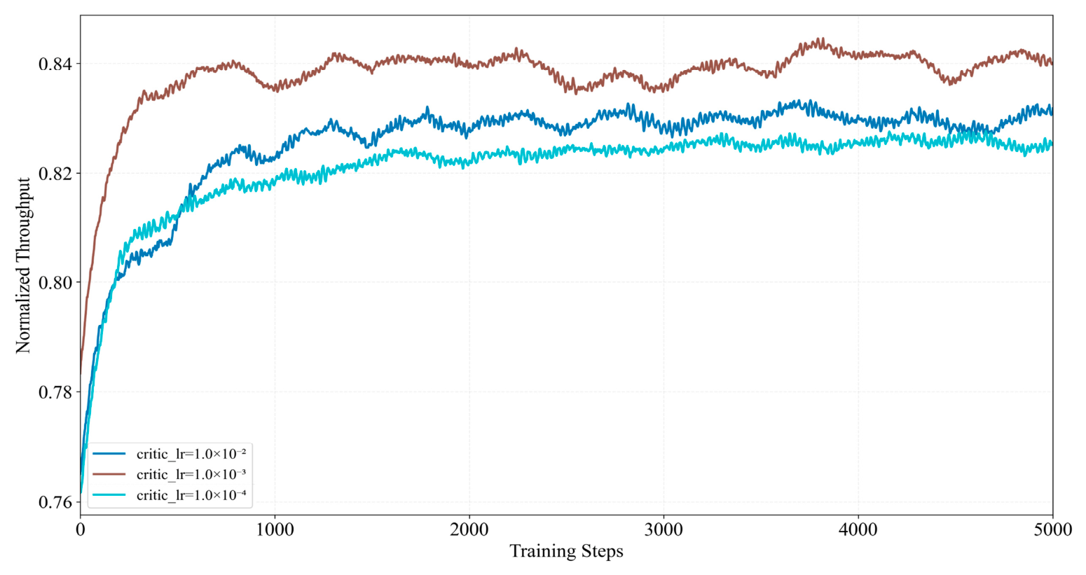
The learning rate ${\alpha }_{\varphi }$ for the value network is a critical hyperparameter in PPO, as it controls the update speed of the network parameters. To determine an appropriate value, this paper investigates the impact of different value network learning rates on algorithm performance in a nonlinear swept-frequency jamming environment.

Figure 2 compares the average reward of the proposed algorithm for ${\alpha }_{\varphi }$ set to 0.01, 0.001, and 0.0001. When ${\alpha }_{\varphi } =0.0001$, the learning rate is too small, leading to slow parameter updates and consequently slow convergence. When ${\alpha }_{\varphi } =0.01$, although the parameters converge rapidly, this setting may cause the algorithm to overshoot the optimum or become trapped in a local optimum, degrading performance. When ${\alpha }_{\varphi } =0.001$, the algorithm achieves both fast convergence and high average reward; therefore, this setting was adopted in subsequent simulations.

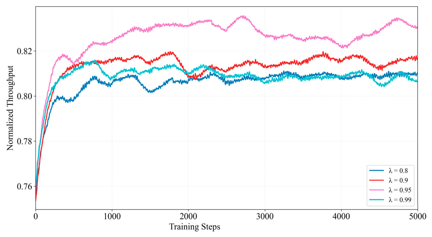
To investigate the impact of the GAE parameter $\lambda$ on the anti-jamming performance of the PPO algorithm in a swept-frequency jamming environment, Figure 3 presents the curves of normalized throughput versus training steps for the PPO algorithm under four different $\lambda$ values. Overall, as training progresses, the normalized throughput gradually increases for all $\lambda$ values, but noticeable differences exist in convergence speed and final performance. When $\lambda =0.8$, the algorithm enters a stable phase after approximately 600 steps, achieving the fastest convergence speed. However, the final normalized throughput stabilizes only around 0.88, with relatively large fluctuations, representing the worst performance. When $\lambda =0.9$, convergence is reached at approximately 1000 steps, but the final normalized throughput increases to 0.90. This indicates that slightly increasing λ and incorporating longer temporal information helps the agent learn to proactively avoid jamming. When $\lambda =0.95$, the final normalized throughput reaches 0.92, the highest among the four groups. This value achieves the best trade-off between bias and variance. It enables the agent to learn the sweeping direction and rate variation patterns of swept-frequency jamming through moderate long-term credit assignment, without causing severe training oscillations due to excessive variance. When $\lambda =0.99$, the final normalized throughput is approximately 0.90. This suggests that in a swept-frequency jamming environment, excessively long credit assignment introduces unnecessary noise, which hampers policy stability.

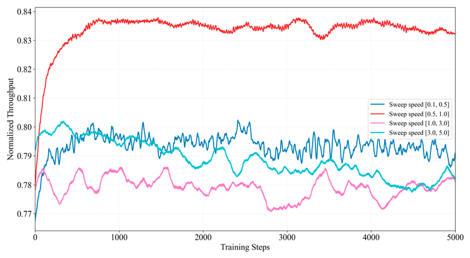
Sweeping rate is a key parameter that determines the jammer’s dynamic characteristics and directly affects the duration of usable spectrum holes. To evaluate the impact of different sweeping rates on the learning performance of the PPO anti-jamming algorithm, four typical rate ranges were configured in the experiment: [0.1, 0.5], [0.5, 1.0], [1.0, 3.0], and [3.0, 5.0]. The results are shown in Figure 4.

Figure 4 shows that the sweeping rate range significantly impacts both the convergence speed and steady-state performance of the algorithm. In the low sweeping rate range [0.1, 0.5], the jammer varies slowly, leading to a slowly changing spectral environment. In such a slowly varying environment, the agent tends to encounter similar state observations for extended periods during early training, resulting in low sample diversity and reduced exploration efficiency. When the sweeping rate range increases to [0.5, 1.0], the algorithm achieves its best performance. Its normalized throughput curve rises quickly, approaching convergence within about 1000 steps, with a steady-state value around 0.835. This indicates that moderate jamming dynamics provide the agent with rich yet predictable spectrum variation, enabling it to learn the frequency-sweeping pattern and acquire a prediction-based channel switching strategy, thus yielding higher anti-jamming gains. However, when the sweeping rate further increases to [1.0, 3.0] and [3.0, 5.0], performance degrades noticeably. Under these two high-rate settings, the convergence speed of the normalized throughput slows down, and the steady-state values drop to approximately 0.784, respectively, significantly lower than those under the medium-low rate settings. A plausible explanation is that the state representation relies solely on jamming observations from the past 5 time slots. When the jammer sweeps at a rate higher than one channel per time slot, the frequency distance of the jamming signal between adjacent time slots increases substantially, making the historical observations insufficient to infer future jamming locations. Furthermore, excessively high sweeping rates cause the jamming channel to change frequently, and the learned strategy tends to switch communication channels repeatedly. The resulting switching overhead further reduces the achievable normalized throughput.

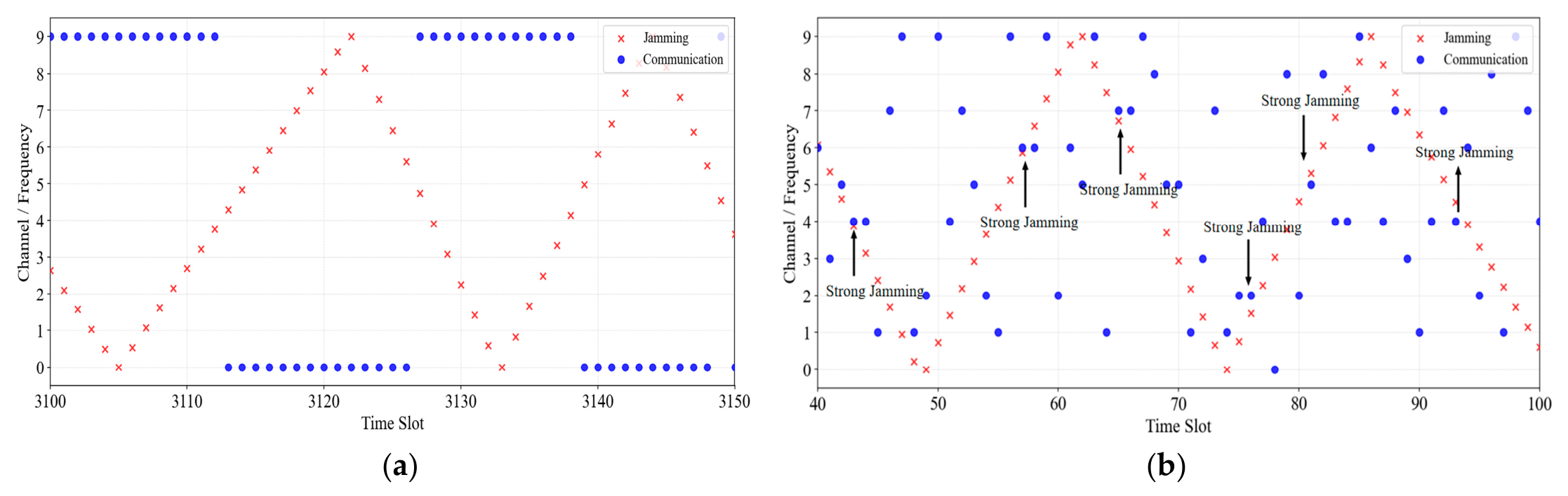
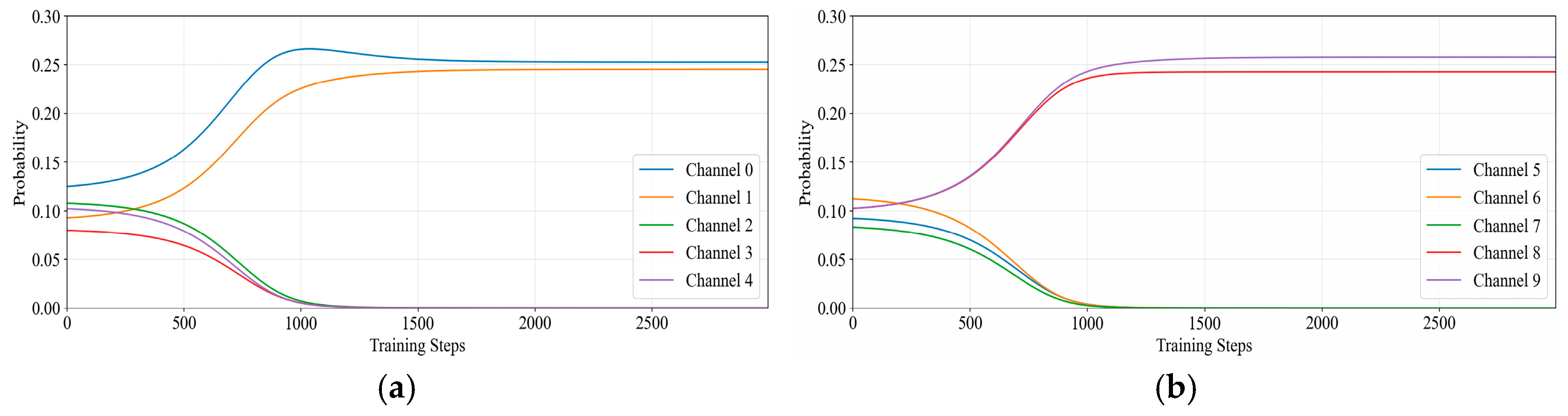
To further examine the learning behavior and decision-making mechanism of the proposed PPO algorithm in a nonlinear swept-frequency jamming environment, this section analyzes the channel selection behavior of both converged and unconverged agents. For each time slot, the selected communication channel, the jamming channel, and the corresponding action probability distribution are recorded. The results are shown in Figure 5 and Figure 6.

Figure 5 compares the time-domain trajectories of the communication channel and the jamming channel during the testing process. It can be seen that the jamming channel scans nonlinearly across channels 0 to 9, with the sweeping rate and direction varying randomly between time slots. In contrast, the communication channel selected by the PPO algorithm does not simply jump away from the channel currently occupied by the jammer but exhibits predictive behavior. This indicates that by learning from the historical jamming trajectory and current jamming dynamics, the PPO algorithm can effectively predict short-term jamming behavior, thereby enabling forward-looking channel selection decisions.

Figure 6 shows the probability distribution over the 10 channels selected by the agent under different states, averaged over all time slots during the testing process. The distribution reveals that the agent does not allocate probability uniformly across channels; instead, it concentrates on edge channels such as 0, 1, 8, and 9. This phenomenon is consistent with the characteristics of nonlinear swept-frequency jamming: the jamming signal reverses direction at both ends of the frequency band, leading to a relatively longer dwell time near the edges, while passing quickly through the middle region. By favoring edge channels, the agent effectively avoids the main jamming energy and reduces the overhead of frequent channel switching caused by sudden changes in jamming direction.

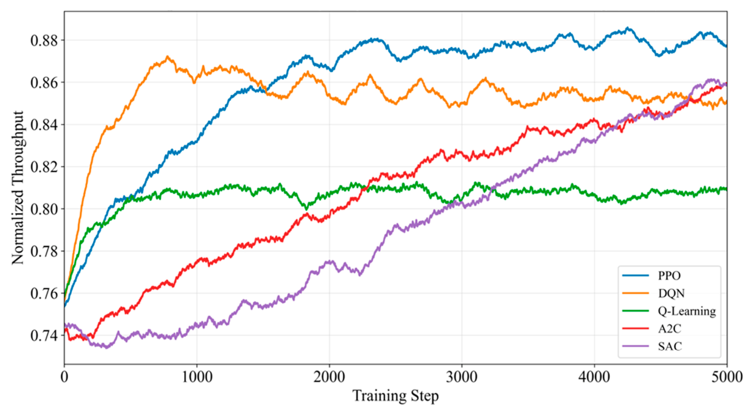
To comprehensively evaluate the performance of the proposed PPO-based anti-jamming algorithm, four baseline algorithms—DQN, Q-Learning, A2C, and SAC (discrete-action version)—were selected for comparative experiments. All algorithms were trained in the same nonlinear swept-frequency jamming environment, with the state space, action space, and reward function kept identical. The simulation results are shown in Figure 7.

As can be observed from Figure 7, the proposed PPO algorithm converges stably after approximately 2000 steps and achieves a final normalized throughput of 0.880, demonstrating excellent jamming avoidance capability and training stability. The SAC algorithm, through its maximum entropy framework and automatic temperature tuning, achieves a good balance between exploration and exploitation; however, its convergence speed is relatively slow and it has not yet entered a stable phase after 5000 steps. The A2C algorithm, which uses one-step TD advantage estimation and synchronous updates, converges slowly and has not yet converged at 5000 steps. The DQN algorithm, under the same hyperparameter settings, shows a convergence speed comparable to that of PPO, but its final normalized throughput is only 0.856 and is highly unstable, which is mainly attributed to DQN’s limited generalization ability in continuous state spaces and the influence of overestimation bias. The Q-Learning algorithm, constrained by the state discretization of the tabular method, struggles to explore the state space sufficiently, and its final normalized throughput only converges to 0.808. The above results indicate that in a nonlinear swept-frequency jamming environment, the policy gradient methods (PPO, SAC, A2C) outperform the value-based methods (DQN, QL) overall. Among them, PPO, by virtue of its clipping mechanism and GAE advantage estimation, achieves the best balance between convergence speed and final performance.

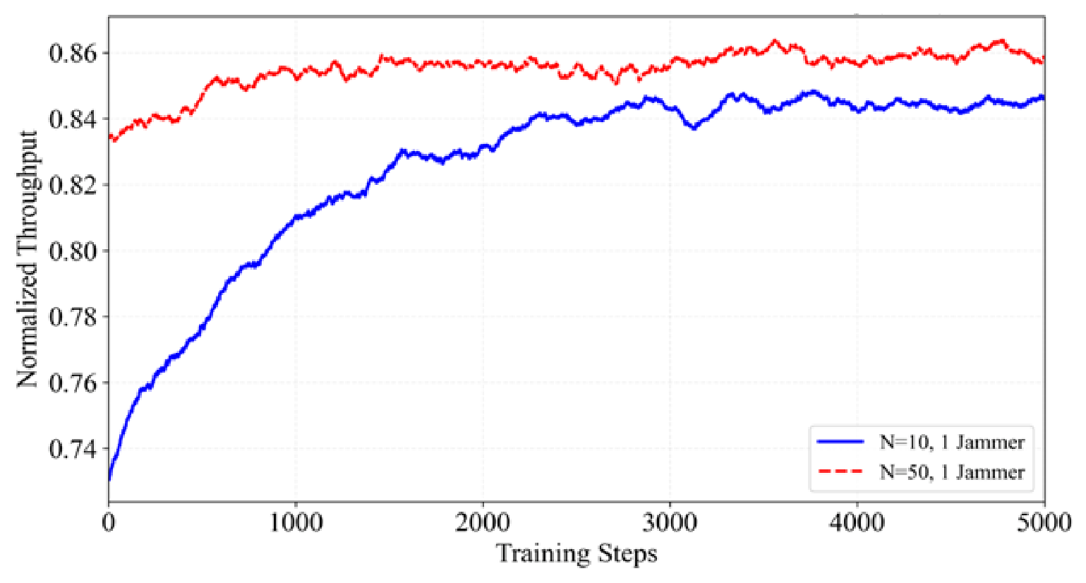
To evaluate the scalability and learning efficiency of the proposed PPO algorithm under different numbers of channels, two comparative experiments were set up in this section: the numbers of channels were 10 and 50, respectively, with the number of jammers kept at 1 in both cases. The results are shown in Figure 8.

From Figure 8, it can be observed that the normalized throughput increases with the number of training steps under both channel configurations; however, significant differences exist in convergence speed and steady-state performance. When $N=10$, the algorithm enters a stable phase after approximately 3000 steps, converging relatively slowly to a final normalized throughput of only 0.840. When $N=50$, the convergence speed is noticeably faster and the performance is stable, with the final normalized throughput converging to 0.860. When the number of channels increases to 50, the same absolute sweeping rate (in channels per time slot) results in the fraction of the band swept per time slot decreasing from 10% to 2%. As the jamming movement becomes relatively slower, the agent can more easily track and proactively avoid the jammer, thereby achieving higher throughput.

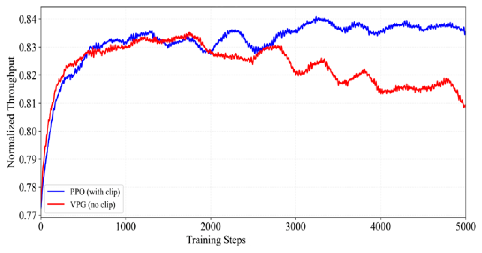
To clarify the contribution of each design element to the algorithm’s performance, we removed the clipping term from the PPO algorithm while keeping all other hyperparameters unchanged. The experimental results are shown in Figure 9. Figure 9 indicates that the algorithm without clipping achieves a final normalized throughput of only 0.815 and exhibits poor stability during training. In contrast, the PPO algorithm with the clipping mechanism converges stably to 0.840. This comparison demonstrates that the clipping mechanism, by limiting the magnitude of policy updates, effectively avoids performance collapse during training and is the key to the PPO algorithm’s high stability and high throughput in nonlinear swept-frequency jamming environments.

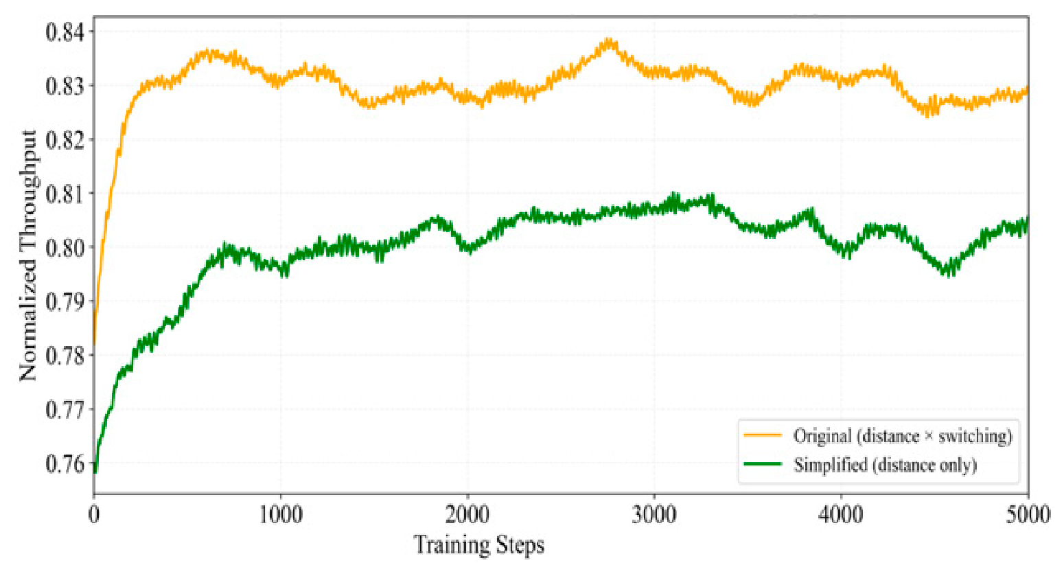
We further compared the complete reward function (which includes both the channel distance penalty term and the switching penalty term, as defined in Equation (7)) with a simplified reward function (which uses only the channel distance penalty term and omits the switching penalty term). The experimental results are presented in Figure 10. As shown, the algorithm with the complete reward function converges faster and achieves a final normalized throughput of 0.910, whereas the algorithm with the simplified reward function only reaches 0.88. This indicates that the introduction of the switching penalty term effectively suppresses unproductive, blind switching behavior and guides the algorithm toward learning a superior channel selection strategy.

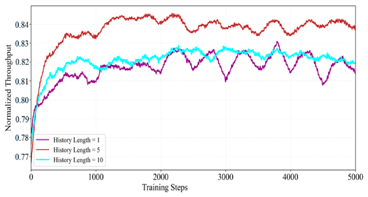
The state representation adopts a sequence of average received powers over the past $L$ time slots. To verify the rationality of this design, we compared three configurations: $L=1$, $L=5$ and $L=10$. From Figure 11, it can be observed that the best performance is achieved with $L=5$, offering a moderate convergence speed. With $L=1$, the historical information is insufficient for the algorithm to accurately predict the evolution of swept-frequency jamming, resulting in slower convergence, poor stability, and a final normalized throughput of only 0.815. With $L=10$, although richer historical information is available, the increased state dimension reduces the exploration efficiency during training, and the steady-state normalized throughput is also slightly lower than that with $L=5$. Therefore, $L=5$ achieves the best balance between information sufficiency and learning efficiency.

5. Conclusions

This study addressed intelligent anti-jamming communication in dynamic nonlinear swept-frequency jamming environments by proposing a novel method based on PPO. The anti-jamming channel selection problem was formulated as a MDP, and a composite reward function was designed. The proposed algorithm rapidly learns the unknown dynamic patterns of malicious jamming and flexibly adjusts its transmission strategy to obtain a near-optimal policy. Simulation results demonstrate that compared with baseline algorithms such as DQN and Q-learning, the proposed PPO-based method achieves faster convergence, higher normalized throughput, and more robust anti-jamming performance. The method exhibits effective jamming tracking and avoidance capabilities under varying sweeping rates and directions.

References

1. Tusha, A.; Arslan, H. Interference Burden in Wireless Communications: A Comprehensive Survey from PHY Layer Perspective. IEEE Commun. Surv. Tutorials. 2025, 27, 2204–2246. [Google Scholar] [CrossRef]
2. Torrieri, D. Principles of Spread Spectrum Communication Systems, 5th ed.; Springer International Publishing: Cham, Switzerland, 2022; pp. 151–203. [Google Scholar]
3. Wang, X.; Wang, J.; Xu, Y.; Chen, J.; Jia, L.; Liu, X. Dynamic Spectrum Anti-Jamming Communications: Challenges and Opportunities. IEEE Commun. Mag. 2020, 58, 79–85. [Google Scholar] [CrossRef]
4. Liu, X.; Shi, M.; Wang, M. Intelligent Frequency Decision Communication with Two-Agent Deep Reinforcement Learning. Electronics 2023, 12, 4529. [Google Scholar] [CrossRef]
5. Qi, J.; Zhang, H.; Qi, X.; Peng, M. Deep Reinforcement Learning Based Hopping Strategy for Wideband Anti-Jamming Wireless Communications. IEEE Trans. Veh. Technol. 2023, 73, 2131–2144. [Google Scholar] [CrossRef]
6. Zhou, Q.; Niu, Y.; Xiang, P.; Li, Y. Intra-domain knowledge reuse assisted reinforcement learning for fast anti-jamming communication. IEEE Trans. Inf. Forensics Secur. 2023, 18, 4707–4720. [Google Scholar] [CrossRef]
7. Zhu, X.; Huang, Y.; Wang, S.; Wu, Q.; Ge, X.; Liu, Y. Dynamic spectrum anti-jamming with reinforcement learning based on value function approximation. IEEE Wirel. Commun. Lett. 2023, 12, 386–390. [Google Scholar] [CrossRef]
8. Liu, X.; Wang, X.; Xu, Y.; Du, Z.; Xu, Y.; Han, H. Lightweight reinforcement learning with state abstraction for dynamic spectrum anti-jamming communications. In Proceedings of the 2024 IEEE Wireless Communications and Networking Conference (WCNC), Dubai, United Arab Emirates, 21–24 April 2024. [Google Scholar] [CrossRef]
9. Ke, Z.; Wang, X.; Du, Z.; Xiong, T.; Xu, Y.; Chen, J. Intelligent frequency reuse for dynamic spectrum anti-jamming: A hybrid-reward-based multi-agent deep reinforcement learning approach. IEEE Wirel. Commun. Lett. 2025, 14, 771–775. [Google Scholar] [CrossRef]
10. Janjar, S.B.; Wang, P. Intelligent anti-jamming based on deep reinforcement learning and transfer learning. IEEE Trans. Veh. Technol. 2024, 73, 8825–8834. [Google Scholar] [CrossRef]
11. Abdolkhani, N.; Hamouda, W. Hierarchical Deep Reinforcement Learning for Robust Access in Cognitive IoT Networks under Smart Jamming Attacks. In Proceedings of the IEEE Global Communications Conference (GlobeCom), Taipei, Taiwan, 7–11 December 2025. [Google Scholar] [CrossRef]
12. Xiong, X.; Hu, S.; Yan, T.; Xing, Z.; Ma, T.; Yin, K.; Wang, J.; Wei, X. Intelligent Jamming Decision-Making System Based on Reinforcement Learning. Comput. Electr. Eng. 2025, 125, 110288. [Google Scholar] [CrossRef]
13. Liu, X.; Xu, Y.; Jia, L.; Wu, Q.; Anpalagan, A. Anti-Jamming Communications Using Spectrum Waterfall: A Deep Reinforcement Learning Approach. IEEE Commun. Lett. 2018, 22, 998–1001. [Google Scholar] [CrossRef]
14. Chen, X.; Ding, H.; Ma, Y.; Li, X.; An, J.; Fang, Y. A Dual-Tier Policy-Oriented Anti-Jamming Scheme Based on Deep Reinforcement Learning. IEEE Trans. Wirel. Commun. 2026, 25, 10652–10668. [Google Scholar] [CrossRef]
15. Geng, J.; Jiu, B.; Li, K.; Zhao, Y.; Liu, H. Joint Optimization of Frequency Selection and Transmit Power for Radar Anti-Jamming using Reinforcement Learning. In Proceedings of the 2024 7th International Conference on Information Communication and Signal Processing (ICICSP), Zhoushan, China, 21–23 September 2024. [Google Scholar] [CrossRef]
16. Jia, L.; Qi, N.; Su, Z.; Chu, F.; Fang, S.; Wong, K. Game Theory and Reinforcement Learning for Anti-Jamming Defense in Wireless Communications: Current Research, Challenges, and Solutions. IEEE Commun. Surv. Tutor. 2025, 27, 1798–1838. [Google Scholar] [CrossRef]
Figure 1. System model.
Electronics 15 02737 g001
Figure 2. Comparison of normalized throughput for the proposed algorithm under different learning rates.
Electronics 15 02737 g002
Figure 3. Comparison of normalized throughput for the proposed algorithm under different GAE λ values.
Electronics 15 02737 g003
Figure 4. Comparison of normalized throughput for the proposed algorithm under different sweeping rates.
Electronics 15 02737 g004
Figure 5. (a) Communication channel and jamming channel trajectories (converged). (b) Communication channel and jamming channel trajectories (non-converged).
Electronics 15 02737 g005
Figure 6. (a) Probability distribution of channel selection (channels 0–4). (b) Probability distribution of channel selection (channels 5–9).
Electronics 15 02737 g006
Figure 7. Comparison of normalized throughput for various algorithms under nonlinear swept-frequency jamming.
Electronics 15 02737 g007
Figure 8. Comparison of normalized throughput for the proposed algorithm under different numbers of channels.
Electronics 15 02737 g008
Figure 9. Impact of the clipping mechanism on the normalized throughput of the proposed algorithm.
Electronics 15 02737 g009
Figure 10. Impact of reward function design on the normalized throughput of the proposed algorithm.
Electronics 15 02737 g010
Figure 11. Impact of historical window length on the normalized throughput of the proposed algorithm.
Electronics 15 02737 g011