Article

Robust Optimal Dispatch Method for a Renewable Energy Base Considering the Impacts of Wind and Photovoltaic Output Uncertainties and Unit Maintenance

1
Guodian Nanjing Automation Co., Ltd., Nanjing 210032, China
2
Nanjing SAC Power Grid Automation Co., Ltd., Nanjing 211153, China
3
State Key Laboratory of Power System Operation and Control, Tsinghua University, Beijing 100084, China
4
Department of Electrical Engineering and Applied Electronics Technology, Tsinghua University, Beijing 100084, China
*
Author to whom correspondence should be addressed.
Electronics 2026, 15(12), 2585; https://doi.org/10.3390/electronics15122585
Submission received: 18 May 2026 / Revised: 10 June 2026 / Accepted: 10 June 2026 / Published: 11 June 2026

Abstract

Medium- and long-term dispatching of renewable energy bases is an important method for ensuring large-scale transmission and consumption. However, most existing medium- and long-term dispatching methods ignore the uncertainties of wind and photovoltaic power output, resulting in excessive maintenance-window margins and insufficient regulation reserves. However, relevant studies that consider such uncertainties are mostly limited to short-term scheduling and are therefore inadequate for medium- and long-term dispatching needs. To this end, a two-stage robust optimal dispatch method for renewable energy bases that considers the impacts of wind and photovoltaic output uncertainties and unit maintenance is proposed. Firstly, the first stage decision variables consist of the on/off and maintenance statuses of thermal power units. Next, the output of each power source is taken as the conventional decision variables in the second stage, while the curtailed wind/photovoltaic power and load shedding are taken as the unconventional decision variables when the balance cannot be achieved by adjusting the power source output under the given wind and solar power output scenarios. In the end, a polyhedron set based on an uncertainty budget was adopted to describe the fluctuations in wind and photovoltaic output, and the minimum scheduling cost in the worst scenarios was solved using the column and constraint algorithm. A renewable energy base in Northwest China was selected as a case to validate the proposed model’s effectiveness. The results show that the proposed model significantly reduces the operating cost in actual operation compared to deterministic optimization and pre-maintenance robust optimization.

1. Introduction

Driven by the “dual carbon” goals, China has built several large-scale renewable energy bases incorporating wind, photovoltaic, thermal, and storage energy in the three northern regions rich in wind and solar resources, which are used to transmit clean electricity to the southeast coastal areas to alleviate the contradiction between energy supply and demand. However, the terrain and climate in the Three-North region are rather complex, and the uncertainty of wind and solar resources, as well as power generation output, is significantly stronger than that in the eastern plain region. Formulating a dispatching and operation plan for large-scale renewable energy bases is critical for maintaining grid stability and maximizing the economic performance of renewable energy bases.
The optimal scheduling problem for multi-capability complementary systems has been widely studied, with a focus on aspects such as multi-type renewable energy collaborative scheduling [1,2], multi-time-scale coupled scheduling [3,4,5], uncertain scheduling considering random fluctuations in power sources and loads [6,7], and optimal scheduling participating in power market transactions [8,9,10], achieving rich research results. We can classify optimization scheduling problems into short-term and medium- and long-term optimization scheduling according to the different optimization time scales. Among them, medium- and long-term optimized dispatching is oriented towards a time scale of several months to several years, providing important guidance for key system operation links such as the arrangement of unit startup and shutdown and maintenance plans, fuel contract signing, and cross-regional transaction decisions. It also offers boundary conditions and operational constraints for short-term optimized dispatching, serving as fundamental support throughout the entire system operation process.
According to different research focuses, the current approaches for medium and long-term scheduling can be divided into two types: optimized scheduling with unit maintenance considerations and optimized scheduling that addresses renewable energy output uncertainty.
Research on medium- and long-term dispatching considering unit maintenance initially focused on constructing accurate maintenance models [11,12,13], and was later gradually integrated with the electricity market [14,15,16]. For instance, reference [15] studied the impact of maintenance plans on operational revenue under the electricity market environment, and reference [16] put forward a bi-level multi-agent approach for generation maintenance decisions in electricity markets, where the transmission system operator (TSO) and generation agents were coordinated to achieve cost minimization and reliability maximization in the context of predictive maintenance.
Although previous studies have comprehensively modeled unit maintenance, they fail to consider how renewable energy output uncertainty affects unit maintenance over medium- and long-term time horizons.
To handle renewable energy output uncertainty in medium- and long-term scheduling, reference [17] constructed a stochastic optimization model. The model used a quasi-probability density function built on two decades of historical wind, solar, and load data. Reference [18] fits the probability density functions of wind and photovoltaic (PV) using instantaneous power data, then samples monthly averages from the same global distribution, ignoring seasonal cycles and temporal correlations. In reference [19], the upper interval bound of renewable energy output was reduced to manually defined optimal and worst-case scenarios. An objective trade-off coefficient was then introduced, converting the original interval optimization problem into a deterministic one that can be solved directly.
Owing to the relatively large middle/long-term prediction errors for renewable energy output, there is a certain gap between the unit maintenance plans obtained by directly using the predicted values for deterministic optimization and the actual dispatching demands. Several studies over the past few years have investigated jointly optimized dispatching methods that consider the impacts of renewable energy uncertainties and unit maintenance. For instance, in reference [20], the authors used kernel density estimation on historical wind and solar measurements and predictions, and generated 1000 scenarios to construct a Wasserstein ambiguity set. Reference [21] proposed an interval-probabilistic worst conditional value-at-risk (IP-WCVaR) based generation maintenance scheduling method to quantify hybrid risks from wind (interval) and load (probabilistic) uncertainty and optimize decisions under the worst-case scenario to enhance power system robustness and economy. Currently, few optimization scheduling studies account for both renewable output uncertainties and unit maintenance in a coordinated manner. Moreover, because of the insufficiency of historical data, output intervals or error distribution functions based on human assumptions are mostly used to describe the uncertainties of renewable energy output. However, the error distribution function hypothesized by humans differs from the actual errors. The simple output range is also difficult to accurately describe the complex changes in the output of renewable energy, resulting in the maintenance and start–stop plans formulated being unable to accurately match the actual operation requirements. In actual operation, the problem of insufficient reserve of adjustment resources remains quite prominent.
To address the above issues, this study takes the wind–PV–thermal–storage–concentrating solar power (CSP) system as the research object and proposes a two-stage robust optimization model that considers the impacts of renewable output uncertainties and unit maintenance. First, decide the maintenance and on–off statuses of thermal power units in the first stage. Second, seek the scenario that maximizes operation cost, and optimize the power output of each source under that scenario. When it is impossible to maintain the balance of power quantity by adjusting the power output, unconventional means such as wind and solar power abandonment and load shedding are adopted to ensure the safe operation of the system. Finally, the fluctuations in renewable energy power are described by a polyhedral set based on the uncertainty budget, and the model is solved using the column and constraint (C&CG) algorithm. Compared with deterministic optimization and robust optimization with preset maintenance plans, the proposed method better meets the dispatching requirements of the renewable energy base and has the lowest total cost in actual operation.

2. Robust Optimization Model Considering Unit Maintenance

The renewable energy base under study comprises five power source types: wind, photovoltaic, CSP, thermal power, and energy storage. Formulate a two-stage robust optimization model that accounts for the thermal unit maintenance plan and the uncertainty of wind and photovoltaic output. Solve it using the Column-and-Constraint Generation algorithm, as shown in Figure 1. In the two-stage robust optimization model, decision-making is performed in two stages. Before renewable output uncertainty is revealed, set the maintenance and on–off statuses of thermal power units in the first stage. In the second stage, after determining the actual renewable output, optimize the dispatch of all power sources, specifically thermal power, CSP, renewable energy curtailment, and load shedding.

2.1. The First-Stage Model

In the first stage, seek the maintenance and start–stop schedule of thermal units that minimizes their start–stop costs. Equations (1)–(3) provide the objective function, which includes start–stop and fixed operating costs. The thermal units’ generation cost is expressed as a linear function.
min C r u n _ c o n s t + C s t a r t
C r u n _ c o n s t = t = 1 T n = 1 N g u g _ n , t b n
C s t a r t = t = 1 T n = 1 N g s t a r t g _ n , t C g _ n , s t a r t
where C r u n _ c o n s t is the fixed cost of power generation by the thermal power unit, C s t a r t is the startup cost of the thermal power unit, T is the number of time periods within the dispatching cycle, N g is the number of thermal power units, u g _ n , t is the thermal power unit on/off status, s t a r t g _ n , t is the thermal unit startup status, b n is the constant term coefficient within the thermal power unit operating cost expression, and C g _ n , s t a r t denotes the thermal power unit startup cost.
The first-stage constraint conditions include the thermal power unit start–stop constraints, as shown in Equations (4)–(7), and the thermal power units’ maintenance constraints, as shown in Equations (8)–(13). Maintenance constraints are divided into three categories: maintenance start time constraints, maintenance duration constraints, and maintenance resource constraints.
s t a r t g _ n , t = u g _ n , t u g _ n , t 1
s t o p g _ n , t = u g _ n , t 1 u g _ n , t
t = 1 T s t a r t g _ n , t = s t a r t g _ n max
t = 1 T s t o p g _ n , t = s t o p g _ n max
t = 1 T 1 1 x g _ n , t = 0
t = T 2 + 1 T x g _ n , t = 0
t = 1 T x g _ n , t = T 3
s g _ n , t = x g _ n , t x g _ n , t 1
t = 1 T s g _ n , t = 1
n = 1 N g x g _ n , t = N max
where u g _ n , t , s t a r t g _ n , t , s t o p g _ n , t , x g _ n , t and s g _ n , t are all 0–1 variables, indicating whether the thermal power unit is operating, starting up, shutting down, undergoing maintenance, or entering maintenance, respectively. s t a r t g _ n max and s t o p g _ n max are, respectively, the maximum allowable startup/shutdown counts for the Nth thermal power unit over the dispatching cycle. T 1 denotes the earliest allowable maintenance time, T 2 is the latest allowable maintenance time, and T 3 is the maintenance duration. N max represents the upper limit on the number of units that can undergo maintenance concurrently in a single period. T denotes the number of periods in the dispatching cycle.

2.2. The Second-Stage Model

After determining actual wind and solar generation, the second-stage model is used to optimize the dispatch of all power sources. Its objective is the minimization of generation cost under the worst-case scenario, which comprises several components: the variable portion of thermal power generation cost, energy storage charging/discharging cost, solar thermal generation cost, renewable curtailment penalty, and load shedding cost. The corresponding objective functions are given in Equations (14)–(19).
max ξ U min y F x , ξ C r u n + C b a t t e r y + C C S P + C c u r + C s h e d
C r u n = t = 1 T n = 1 N g a n P g _ n , t Δ t
C b a t t e r y = t = 1 T α b a t t e r y c h a P b a t t e r y , t c h a + α b a t t e r y d i s P b a t t e r y , t d i s Δ t
C C S P = t = 1 T k c s p P c s p , t Δ t
C c u r = t = 1 T α c u r P w i n d _ c u r , t + α c u r P p v _ c u r , t Δ t
C s h e d = n = 1 T α s h e d P l o a d _ s h e d , t Δ t
where C r u n is the variable part of the thermal power units’ generation cost, C b a t t e r y denotes the energy storage charge/discharge cost, C C S P denotes the power generation cost of CSP, C c u r is the penalty cost of renewable energy curtailment, and C s h e d represents the penalty cost of load shedding. T is the number of time periods within the dispatching cycle. Δ t is the duration of the dispatching period. N g is the number of thermal power units, a n is the coefficient of the first term in the operating cost of thermal power, P g _ n , t is the output of the thermal power unit. The energy storage charging and discharging cost coefficients are denoted by α b a t t e r y c h a and α b a t t e r y d i s , respectively. Similarly, the energy storage charging and discharging power are denoted by P b a t t e r y , t c h a and P b a t t e r y , t d i s . k c s p is the cost coefficient of CSP, and P c s p , t is the output power of CSP. α c u r is the renewable energy curtailment cost coefficient. P w i n d _ c u r , t and P p v _ c u r , t are the power for wind and solar power curtailment. α s h e d is the load shedding cost coefficient, and P l o a d _ s h e d , t is the load-shedding power.
The second-stage constraints encompass the output limits of thermal, wind, and PV generation, the energy storage and CSP operating restrictions, as well as the overall system balance.
Thermal unit output constraints appear in Equation (20). It should be noted that during maintenance periods, the maximum feasible output of a thermal unit decreases. In medium- and long-term dispatching with a time step of days or more, the ramp-up capacity of thermal power units is fully capable of supporting the units to climb from the lowest technical output to the highest technical output between two adjacent periods. Therefore, the ramp-up constraint of thermal power units is no longer considered in medium- and long-term dispatching.
u g _ n , t P g _ n min P g _ n , t u g _ n , t P g _ n max x g _ n , t Δ P g _ n f i x
where P g _ n min and P g _ n max are, respectively, the maximum and minimum power of the Nth thermal power unit, P g _ n , t is the power of the Nth thermal power unit during period t, and Δ P g _ n f i x represents how the Nth thermal power unit’s maintenance affects its maximum technical output. If the shutdown maintenance is adopted, add a constraint Δ P g _ n f i x = P g _ n max or u g _ n , t + x g _ n , t 1 to prevent the unit from starting up during maintenance. The constraints of CSP plant operation are shown in Equations (21)–(28). Here, a parabolic trough/Fresnel CSP plant model is used. The heat generated by the unit can be released from the heat storage tank or absorbed by the collector, but the charging and releasing of heat cannot occur simultaneously.
E min E t E max
E t + 1 = E t + η c s p c h a ω c s p , t c h a H c s p , t c h a Δ t ω c s p , t d i s H c s p , t d i s Δ t / η c s p d i s
0 H c s p , t c h a ω c s p , t c h a H c s p , max c h a
0 H c s p , t d i s ω c s p , t d i s H c s p , max d i s
ω c s p , t c h a + ω c s p , t d i s 1
H c s p , t i n = H c s p , t c h a + H c s p , t g H c s p , t c u r
P c s p , t = β c s p H c s p , t d i s + H c s p , t g
u C S P , t P c s p min P c s p , t u C S P , t P c s p max
where E t is the heat storage capacity of the CPS during period t, E max and E min are the upper and lower limits of the heat storage capacity of the CPS. η c s p c h a and η c s p d i s are the heat charging and discharging efficiency of the CPS. The efficiency associated with charging and discharging the heat are denoted by η c s p c h a and η c s p d i s . The heat charging and discharging states are denoted by 0–1 variables ω c s p , t c h a and ω c s p , t d i s , which can not be one simultaneously. Similarly, the heat charging and discharging power are denoted, respectively, by H c s p , t c h a and H c s p , t d i s , the maximum heat charging and discharging power are denoted, respectively, by H c s p , max c h a and H c s p , max d i s . H c s p , t i n is the heat received by the CPS from the collector, H c s p , t c u r is the wasted heat, and H c s p , t g is the heat directly used for power generation.  P c s p , t denotes the power of the CPS in period t, β c s p presents the thermoelectric conversion efficiency of the CPS. P c s p max and P c s p min are the maximum and minimum limits of the output of the unit. The 0–1 variable u C S P , t represents the CSP operating state.
The constraints of the wind and solar output constraints are shown in Equations (29)–(32), which limit the actual wind and solar output to not exceed the predicted value and restrict the renewable curtailment to not be less than zero.
P w i n d _ n , t p r e d = P w i n d _ n , t + P w i n d _ c u r , t
P p v , t p r e d = P p v , t + P p v _ c u r , t
0 P w i n d _ c u r , t P w i n d _ n , t p r e d
0 P p v _ c u r , t P p v , t p r e d
where P w i n d , t and P p v , t are the actual outputs of the wind farm and photovoltaic power station during the t period, P w i n d _ n , t p r e d and P p v _ n , t p r e d represents the predicted power of the wind farm and photovoltaic power station during the t period, P w i n d _ c u r , t and P p v _ c u r , t represents the renewable curtailment.
The constraints of energy storage operation are shown in Equations (33)–(37), which limit the capacity and charging/discharging power of the energy storage equipment to meet the physical constraints.
S O C min S O C t S O C max
S O C t + 1 = S O C t + η b a t t e r y , t c h a ω b a t t e r y , t c h a P b a t t e r y , t c h a Δ t ω b a t t e r y , t d i s P b a t t e r y , t d i s Δ t / η b a t t e r y , t d i s
0 P b a t t e r y , t c h a ω b a t t e r y , t c h a P b a t t e r y , max c h a
0 P b a t t e r y , t d i s ω b a t t e r y , t d i s P b a t t e r y , max d i s
ω b a t t e r y , t c h a + ω b a t t e r y , t d i s 1
where S O C t is the charge quantity of the energy storage device in period t. The maximum and minimum charge quantities of the energy storage device are denoted by S O C max and S O C min . The efficiency associated with charging and discharging the energy storage device is denoted by η b a t t e r y , t c h a and η b a t t e r y , t d i s . The power associated with charging and discharging the energy storage device is denoted by P b a t t e r y , t c h a and P b a t t e r y , t d i s . The maximum power associated with charging and discharging the energy storage device is denoted by P b a t t e r y , max c h a and P b a t t e r y , max d i s . The energy storage charging and discharging states are denoted by the 0–1 variables, ω b a t t e r y , t c h a and ω b a t t e r y , t d i s , neither of which can be equal one simultaneously.
The constraints of system operation are as shown in Equations (38)–(40). Equation (38) is the energy balance constraint, which requires that over the entire dispatch period, the total generated energy equals the total consumed energy. Equation (39) states the power balance condition: the generation output must be equal the load demand minus any shed load, for every time step.
t = 1 T ( n = 1 N g P g _ n , t + P w i n d , t + P p v , t + P c s p _ n , t + P b a t t e r y , t c h a P b a t t e r y , t c h a ) Δ t = t = 1 T P l o a d , t P l o a d _ s h e d , t Δ t
n = 1 N g P g _ n , t + P w i n d , t + P p v , t + P c s p _ n , t + P b a t t e r y , t c h a P b a t t e r y , t c h a = P l o a d , t P l o a d _ s h e d , t
n = 1 N g u g _ n , t P g _ n max x g _ n , t Δ P g _ n f i x n = 1 N g P g _ n , t R s
where P l o a d , t is the average load during period t, P l o a d _ s h e d , t is the shedding load during period t, and R s is the reserve capacity.

2.3. Construction of Uncertainty Sets

Common types of uncertainty sets include box uncertainty sets, ellipsoidal uncertainty sets, polyhedral uncertainty sets, uncertainty sets constructed on the basis of data-driven approaches, etc. Among them, the box-type uncertainty set is overly simplistic. Not only is it difficult to describe the complex changes in wind and solar power output, but the fixed output range also makes the robust optimization overly conservative, increasing the scheduling cost. The construction of uncertainty sets based on data-driven methods can solve the problem of overly conservative box-type uncertainty sets and is a widely applied approach in recent years. For instance, in reference [22], after cleaning the data with GNN, a pair convex hull uncertainty set (PCHUS) was constructed, and the model conservation was adjusted by changing the confidence level. Although this method can accurately model the uncertainty of renewable energy output, with only one year of measured data, the convex hull range is extremely small, seriously underestimating the uncertainty of renewable energy output, which may lead to the loss of robustness of the generated scheduling strategy. Therefore, the uncertainty set constructed based on data-driven methods is applicable in the research scenarios of this paper. Taking all factors into consideration, this paper adopts an uncertainty budget to construct the polyhedral uncertainty set.
Based on the predicted output of wind and photovoltaic power, the output of wind and photovoltaic power may fluctuate upward or downward at the same time. Ideally, when there are fluctuations in wind and photovoltaic power, the processing of other power sources will be changed in the order of the smallest increase in cost. When the output of wind and photovoltaic power fluctuates upward, the output of thermal power and photovoltaic thermal power should be reduced first. Then, the discharge power of energy storage decreases, and the charging power increases. If the power balance still cannot be achieved, we have to curtail wind and photovoltaic power output. During this process, the operating cost first decreases and then increases, and the power reduction range is n = 1 N g P g _ n , t u g _ n , t P g _ n min + P c s p _ n , t u C S P , t P c s p min + P b a t t e r y , t d i s .
When the output of wind and photovoltaic fluctuates downward, first reduce the charging power of energy storage and increase the discharging power. Then increase the output of CSP and thermal power. If the power balance still cannot be achieved, part of the load needs to be shed. During this process, although the operating cost first decreases and then increases, the cost reduction only occurs at the stage when the charging power of the energy storage is reduced. Once the energy storage switches to discharging, the cost begins to increase; that is, the power fluctuation range of the cost reduction is the same as that of the charging power at this time, which is P b a t t e r y , t c h a . Due to the energy storage power limitation and the temporal correlation brought about by the charging and discharging behavior, the power fluctuation range of cost reduction is much smaller than the upward fluctuation of wind and solar power.
It can be seen that when only the cost changes caused by the fluctuation of wind and solar output at a certain moment are analyzed, the downward deviation of wind and solar output is more likely to lead to cost increases, and the increase in cost is even greater. When analyzing the cost changes caused by the fluctuations in wind and solar output over a period of time, the downward fluctuations in wind and solar output will lead to an increase in the power generation of thermal power and solar thermal power, as well as a rise in power generation costs. At the same time, the load that cannot be met through regulation measures needs to be shed, which greatly increases the operating costs of the system. When the output of wind and solar power fluctuates upward, the power generation of thermal power and solar thermal power decreases, and the power generation cost drops. Although there may be costs of wind and solar power curtailment, these costs are far lower than the load-shedding costs. From the perspective of system operation safety, it is also hoped to avoid load shedding as much as possible. Therefore, in this article, only the situation of rural fluctuations in wind and solar output is considered.
The fluctuation range of wind and photovoltaic output is described by using the polyhedral uncertainty set based on the uncertainty budget. The fluctuation level of wind and solar output is limited by the uncertainty budget and the maximum deviation ratio. The degree of conservatism in robust optimization is adjusted. The specific form of the uncertainty set is shown in Equation (41).
U = Δ w i n d t , Δ p v t 0 Δ w i n d t 1 , t = 1 T Δ w i n d t Γ w i n d , P w i n d , t p r e d Δ w i n d t Δ P w i n d , t max 0 , Δ P w i n d , t max = β w i n d × P w i n d , t p r e d 0 Δ p v t 1 , t = 1 T Δ p v t Γ p v , P p v , t p r e d Δ p v t Δ P p v , t max 0 , Δ P p v , t max = β p v × P p v , t p r e d
where Δ w i n d t and Δ p v t are the output deviation of wind power and photovoltaic power during the t period, Γ w i n d and Γ p v are the uncertainty budgets of wind power and photovoltaic power, β w i n d and β p v are the maximum deviation ratio of wind power and photovoltaic power, Δ P w i n d , t max and Δ P p v , t max are the maximum deviation of wind power and photovoltaic power during the t period, P w i n d , t p r e d and P p v , t p r e d represent the predicted power of wind power and photovoltaic power during the t period.

3. Solution of the Robust Optimization Model

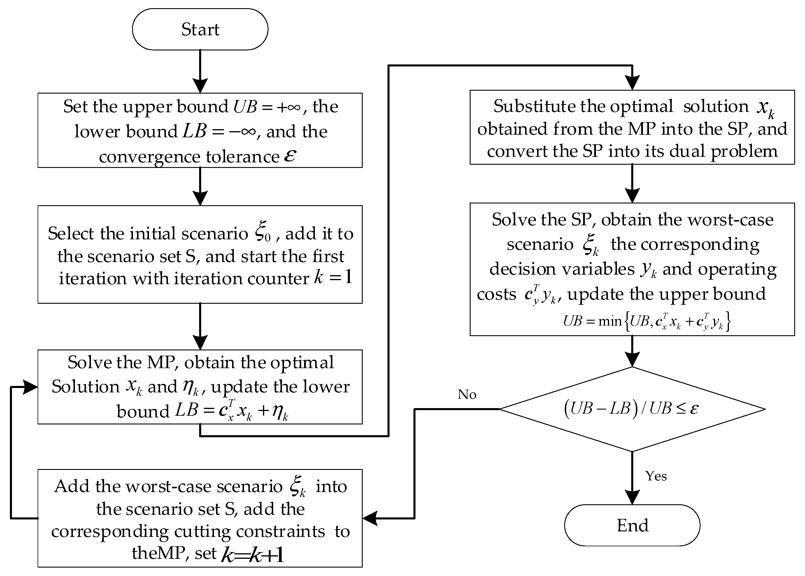
The C&CG algorithm is adopted to solve the two-stage robust optimization model. The model constructed in the previous section is split into the Master Problem (MP) and the Subproblem (SP). The MP makes the optimal decision under limited scenarios and seeks the minimum operating cost in a specific scenario. The SP finds the worst scenario that maximizes the operating cost under the current decision and adds the corresponding variables and constraints of this scenario to the MP. Through the iterative solution of the MP and the SP, the scenario set of the MP is continuously enriched to approach the optimal solution of the original problem.
The matrix form of the MP is shown in Equation (42).
min c x T x + η D y k = d + D x x + D ξ ξ k E y k e + E x x + E ξ ξ k y k 0 c y T y k η
where c x is the coefficient vector of the objective function in the first stage, x is the decision variable of the first stage, y k is the decision variable of the second stage in the uncertainty scenario k, ξ k is the value of the uncertainty variable in the uncertainty scenario k, D , D x , D ξ , E , E x and E ξ are the coefficient matrix, d and e are the constant sequence vector, η is the maximum second-stage cost in multiple uncertainty scenarios, which are obtained by solving the subproblem.
The matrix form of the SP is shown in Equation (43).
max ξ U   min y   c y T y D y = d + D x x k + D ξ ξ E y k e + E x x k + E ξ ξ y 0
where c y is the coefficient vector of the objective function in the second stage; x k is the first-stage decision variable in the uncertainty scenario k; y is the second-stage decision variable; ξ is the value of the uncertainty variable in the uncertainty set U; D , D x , D ξ , E , E x , and E ξ denote the coefficient matrix; and d and e denote the constant sequence vector.
Since the minimax form of the subproblem cannot be directly solved by commercial solvers, it is necessary to transform the minimax problem within the subproblem into a dual maximum problem. In the sub-problem, the only binary variables are the energy storage charge and discharge identifier and the CSP charge and release heat identifier. These two sets of binary variables are physically repelling each other. Even if the relaxation is a continuous variable, its true charge and discharge state can still be determined, thereby guiding the correct search direction for the most severe scenarios. Furthermore, the most severe scenarios found in the sub-problems still need to be precisely solved again in the main problem using the unrelaxed model. Therefore, the relaxation in the sub-problems will not affect the precise solution of the overall model. The 0–1 variables in the sub-problem are directly relaxed into continuous variables between 0 and 1, and then transformed into the single-layer max form shown in Equation (44) for solution.
max ξ U , π , μ π T d + D x x k + D ξ ξ + μ T e + E x x k + E ξ ξ π T D + μ T E c y T μ 0
where π and μ are dual vectors. The meanings of the remaining variables are the same as those in Equations (42) and (43).
Figure 2 provides the complete iterative process of the C&CG algorithm.

4. Results and Discussion

4.1. Example Setting

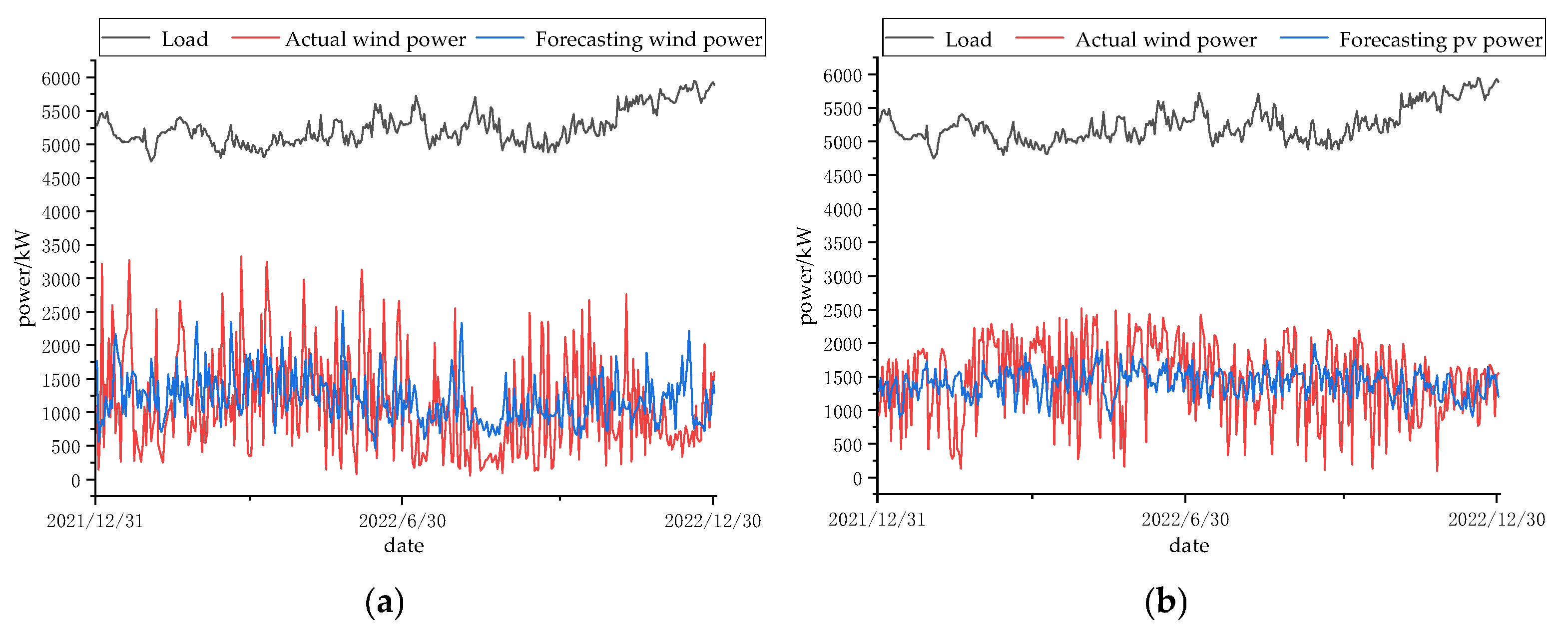
Taking the external transmission system of a large multi-energy base of wind, solar, thermal, storage, and heat in the northwest as an example, the effectiveness of the medium- and long-term dispatching strategy proposed considering the impacts of wind and photovoltaic output uncertainties and unit maintenance is verified. The base includes seven thermal power units with a total capacity of 4000 MW, alongside 4000 MW of wind turbines, 7000 MW of photovoltaic units, 200 MW of solar thermal units, and a 2000 MW/8000 MWh energy storage system. It is set that the thermal power unit undergoes a shutdown for maintenance once a year, with each maintenance lasting 15 days. Maintenance is not allowed in the first and last months of each year. Table 1 provides the other parameters of the thermal power unit. The cost of charging and discharging energy storage is 10 yuan per MWh, the cost of solar thermal power generation is 15 yuan per MWh, the penalty for wind and solar power abandonment is 5000 yuan per MWh, and the penalty for load shedding is 15,000 yuan per MWh. In the calculation example, the dispatching period is one year (365 days), and the dispatching time step is set to 1 day. Figure 3 provides the average daily power of the load, wind, and photovoltaic generation.
Table 1. Parameters of thermal power units.
Num P g _ n max  (MW) P g _ n min  (MW) a n  (Yuan/MW) b n  (Yuan) C g _ n , s t a r t  (Yuan)
11000300198.16260.950,000
21000300198.16260.950,000
3500200115.86617.835,000
4500200115.86617.835,000
5500200115.86617.835,000
6300150168.44242.020,000
720080150.04000.010,000
where, P g _ n min and P g _ n max are the highest and lowest technical outputs of the Nth thermal power unit. a n and b n represent the coefficient of the first term and the constant term coefficient in the operating cost of thermal power. C g _ n , s t a r t is the startup cost of the thermal power unit.
Design seven comparison scenarios for the purpose of verifying the proposed robust optimization scheduling method, considering the maintenance of thermal power units and the uncertainty of wind and photovoltaic output. The maintenance plans and start–stop plans of thermal power units obtained from each scenario were applied to the actual measurement scenarios to simulate the performance of these methods in actual operation. The seven comparison scenarios are set as follows:
Scenario 1 (Deterministic Optimization–Collaborative Maintenance): Considering the maintenance plan for thermal power units, based on the wind and photovoltaic predicted values, carry out deterministic optimization and obtain the expected dispatching cost, the maintenance plan, and the start–stop plan for thermal power units.
Scenario 2 (Robust Optimization–Fixed Maintenance–Unidirectional Fluctuating Uncertainty Budget Set): The maintenance plan for thermal power units is artificially arranged and forced to be carried out during the period with the minimum net load. Here, the net load is calculated using the wind and photovoltaic predicted values. Construct the budget set allowing bidirectional fluctuations, take the uncertainty budget as 100, carry out robust optimization, and obtain the expected dispatching cost, the maintenance plan, and the start–stop plan for thermal power units.
Scenario 3 (Random Optimization—Collaborative Maintenance): The wind and photovoltaic predicted values minus the wind and photovoltaic measured values result in the prediction errors. Randomly sample from the errors and generate several new scenarios from these errors, cluster them into 50 categories using the K-Means method, and then conduct random optimization to obtain the expected dispatching cost, the maintenance plan, and the start–stop plan for thermal power units.
Scenario 4 (Robust Optimization–Collaborative Maintenance–Box-type Uncertainty Set): Calculate the 10% and 90% quantiles of historical measured values of wind and solar power, construct a box-type uncertainty set, conduct robust optimization, and obtain the expected dispatching cost, the maintenance plan, and the start–stop plan for thermal power units.
Scenario 5 (Robust Optimization–Collaborative Maintenance–Bidirectional Fluctuating Uncertainty Budget Set): Based on the wind and photovoltaic predicted values, construct an uncertainty budget set that allows bidirectional fluctuations in wind and solar output. Taking the uncertainty budget as 100 and taking the maximum deviation of the ratio of wind power and photovoltaic power as 0.3, conduct robust optimization, and obtain the expected dispatching cost, the maintenance plan, and the start–stop plan for thermal power units.
Scenario 6 (Robust Optimization–Collaborative Maintenance–Unidirectional Fluctuating Uncertainty Budget Set): The method proposed in this paper. Builds the uncertainty budget set that only operates with downward fluctuations, takes the uncertainty budget as 100, takes the maximum deviation ratio of wind power and photovoltaic power as 0.3, conducts robust optimization, and obtains the expected dispatching cost, the maintenance plan, and the start–stop plan for thermal power units.
Scenario 7: The maximum deviation ratio of wind and photovoltaic power is set to 0.6, and the rest is the same as Scenario 6.

4.2. Result Analysis

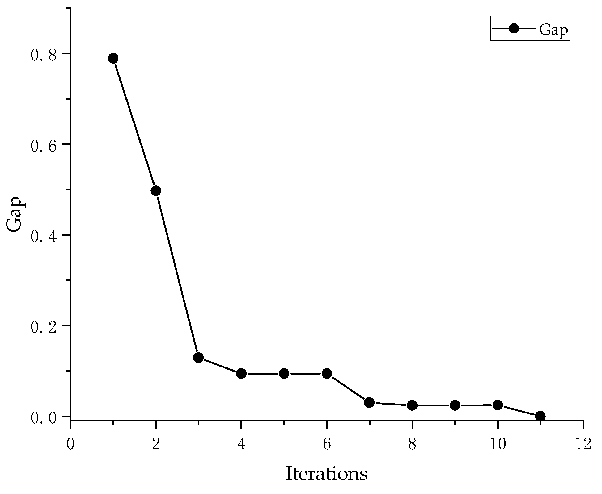
Set the convergence tolerance to 0.1%, the time limit for solving the main problem to be 7200 s, the time limit for solving the sub-problem to be 60 s, and the remaining parameters to adopt the default Settings of Gurobi 11.0. Table 2 provides the simulation results of the seven scenarios. The convergence curve of Scenario 6 is shown in Figure 4.
Table 2. Seven scenarios optimization results.
Scenarios C t o t a l exp e c t C t o t a l a c t u a l C 1 C 2 C b a t t e r y C c u r C s h e d η R E η l o a d
130.872289.19000.0260523.27100.64570.294764.64690.0263%0.9372%
235.354352.30130.0151524.58730.63710.723026.03590.0645%0.3775%
332.177748.27370.0347524.54380.64610.843021.90760.0752%0.3176%
4510.828136.73040.0023526.00570.63871.97757.81360.1764%0.1133%
533.494552.09560.0203523.99050.64500.387026.74590.0345%0.3878%
635.524644.46040.0210524.49020.64420.963018.03970.0859%0.2615%
786.069328.75150.0218025.23230.65090.90111.64720.0804%0.0239%
where, C t o t a l presents the expected total cost. C t o t a l a c t u a l denotes the actual total cost. C 1 presents the startup and shutdown costs of thermal power, and C 2 presents the other costs of thermal power. C b a t t e r y is the operating cost of energy storage. C c u r is the penalty cost for wind and solar power curtailment. C s h e d is the penalty cost for load shedding. The unit of all the above variables is 100 million yuan. η R E is the renewable energy curtailment rate. η l o a d is the load shedding rate.
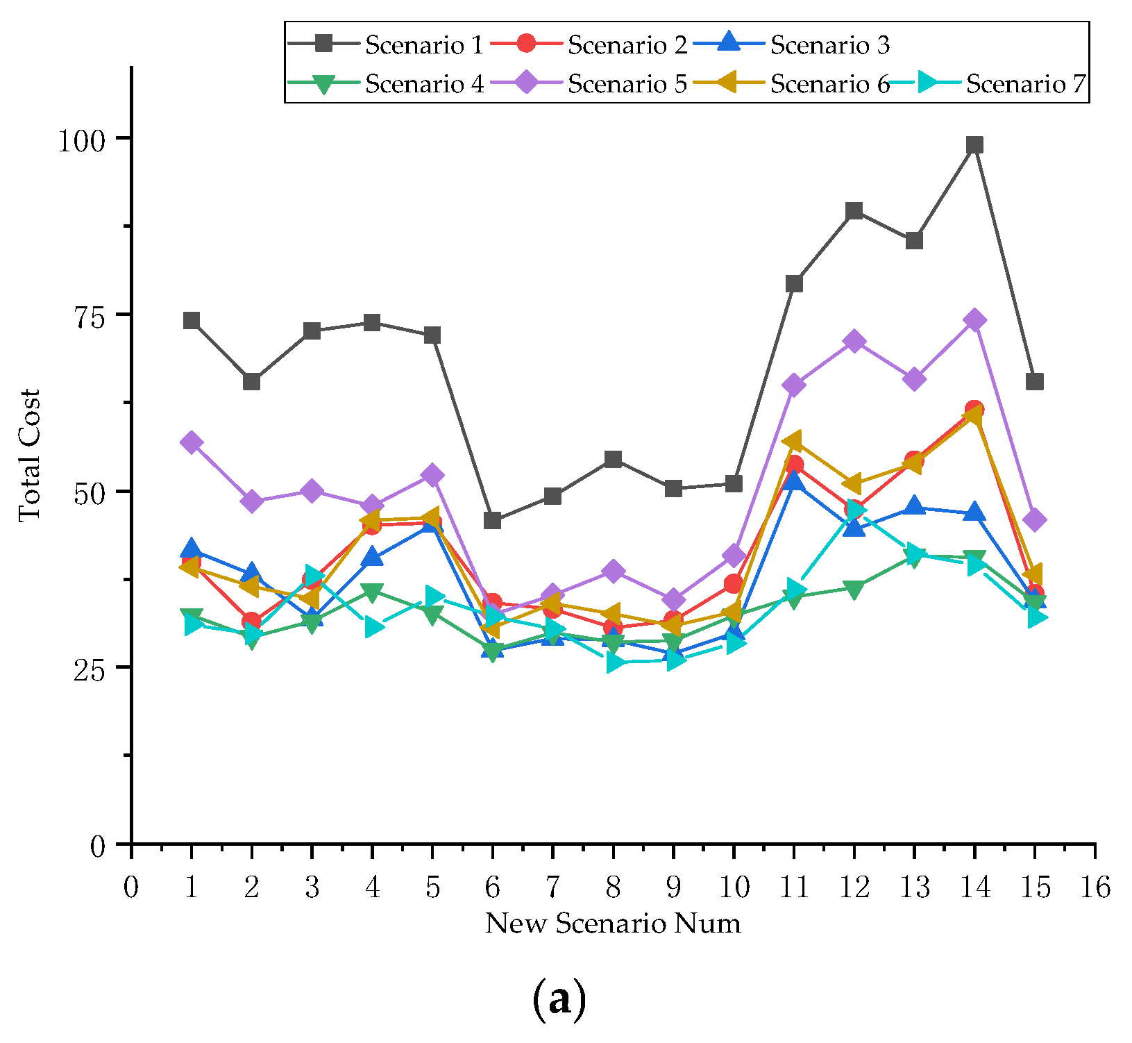
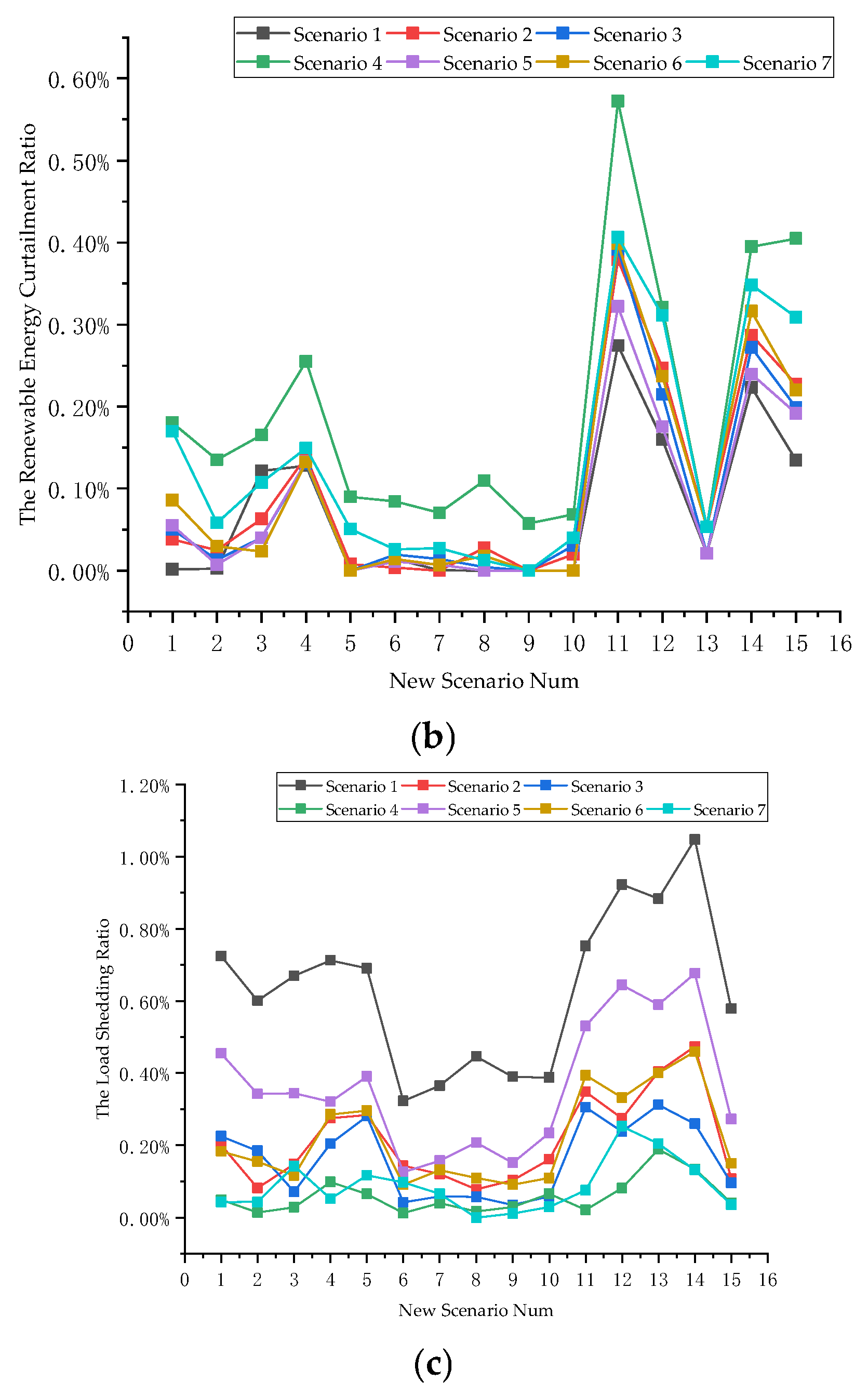
The wind and photovoltaic predicted values minus the wind and photovoltaic measured values result in the prediction errors. Randomly sample from the errors and generate five new scenarios from these errors. Subsequently, multiply the errors by 0.8 and generate five new scenarios; multiply the errors by 1.2 and generate five new scenarios. Now there are a total of ten scenes, which are numbered from 1 to 15, respectively. The operating cost, load shedding rate, and renewable energy curtailment rate are used as metrics to characterize the actual operational performance of the seven scenarios. Figure 5 gives the results.
The total cost of Scenario 1 is the lowest, while the thermal power units’ startup/shutdown cost is the highest. It is evident that the units start and stop frequently. Through refined startup and shutdown strategies, the thermal power generation cost and the energy storage operation cost have been effectively reduced. However, this measure reduces the ability of thermal power units to regulate the fluctuations of wind and solar power. When the wind and photovoltaic output fluctuations exceed the limited regulation capacity of thermal power and energy storage, the system has to shed load to maintain power balance, which leads to the worst performance of this method in actual scenarios, with the highest load shedding rate and the highest total cost among the seven scenarios.
Scenario 3 conducts random optimization based on randomly sampled scenarios. By minimizing the expected cost within each scenario, the optimization framework guarantees robust performance over all tested cases. However, in more severe scenarios, such as the measured scenarios, Scenarios 1, 3, 14, and 15, its performance is not as good as that of Scenario 7.
Scenarios 2, 4, 5, 6, and 7 all adopt robust optimization, but due to the different uncertainty sets, the expected cost and the actual operating cost obtained also have significant differences.
Scenario 2 forces thermal power units to undergo maintenance during the period of minimum net load, which greatly limits the thermal power units’ regulation capacity. Although the expected cost is not much different from that of Scenario 6, in actual operation, the cost of Scenario 2 is higher than the cost of Scenario 6.
Scenario 4 adopts a box-type uncertainty set for robust optimization, which is the most conservative. Therefore, the expected cost is much higher than that of other scenarios. However, due to its excessive conservatism, the number of thermal power units that start and stop is extremely small, almost maintaining a constant state. The thermal power generation cost is extremely high, and the cost of renewable energy curtailment rate is also extremely high during actual operation. Correspondingly, this scheme significantly reduces the load shedding rate.
The uncertainty constructed in Scene 5 takes into account both the situation where the actual wind and photovoltaic output fall short of the forecast value and the situation where it exceeds the forecast value. Compared with Scene 6, it has a lower degree of conservatism, but the operating cost and load shedding rate are higher in the actual scene.
Compared with Scene 6, Scene 7 increases the maximum allowable fluctuation of wind and solar output, which is equivalent to increasing the model’s conservatism. This significantly raises the expected cost of Scene 7 and greatly reduces the actual operating cost.
By comparing the start–stop costs and power generation costs of thermal power in seven scenarios, it can be seen that robust optimization tends to reduce the start–stop frequency of thermal power units, maintain more units in online operation to cope with the uncertainty of wind and solar power output, and exchange higher power generation costs for system robustness.
A comprehensive comparison shows that the uncertainty of renewable energy output has a much greater impact on the operating cost of the system than the maintenance plan. Integrating the maintenance plan with the uncertainty of wind and solar power into the framework of optimized dispatching can rationally allocate and regulate resources in the prediction stage, effectively reduce the risk of load shedding in actual operation, and achieve a harmonious unity of economy and reliability.

4.3. Comparative Analysis of Maintenance Plans

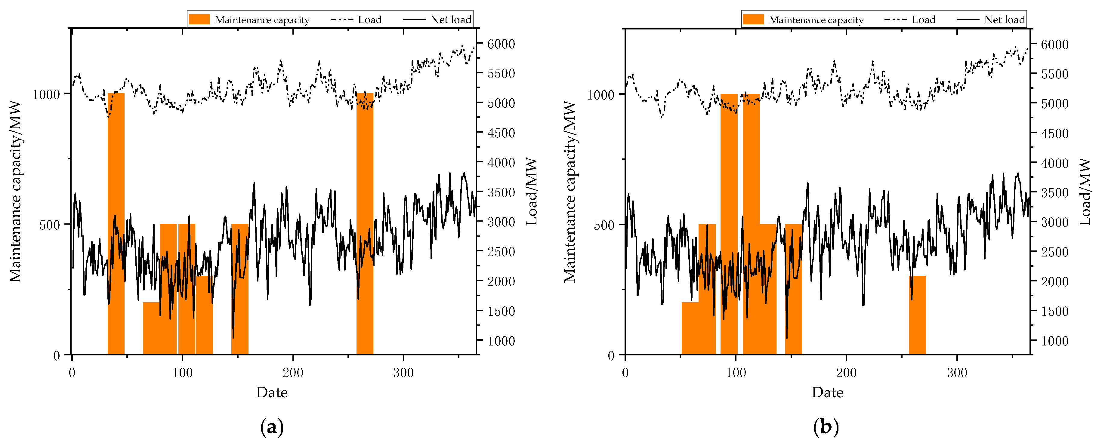
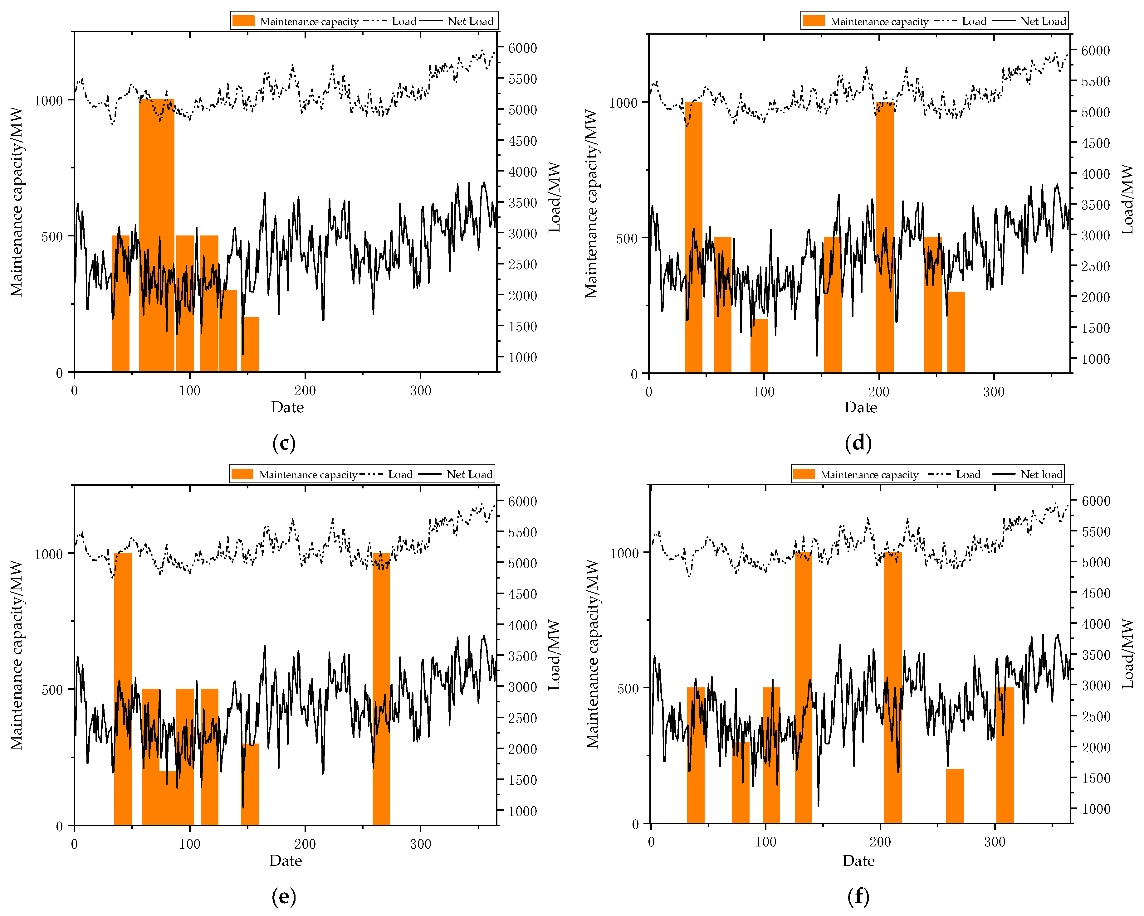
The maintenance plans for the units obtained in each scenario are shown in Figure 6. The net load in the figure is equal to the load minus the predicted output of wind and solar power.
In Scenario 2, the maintenance plan for thermal power units is determined in advance before the optimization scheduling begins, and the maintenance of the units is forced to be carried out during the period when the net load output is at its minimum. As shown in Figure 6b, the smaller the net load, the greater the maintenance capacity arranged.
Both Scenario 1 and Scenario 3 arrange the maintenance of the units based on the predicted values of wind and solar output, as shown in Figure 6a,c. The obtained maintenance plans partially overlap with those in Scenario 2, and the similarity is relatively high. The difference is that Scenario 2 takes into account multiple possible scenarios of wind and solar output, concentrating the maintenance plan during periods when the load level is relatively stable, thus avoiding the period in the second half of the year when the load and renewable energy both fluctuate sharply, leading to an increase in regulation demand.
Scenarios 4, 5, and 6 all adopt robust optimization to arrange the unit maintenance plan. In Scenario 4, the maximum wind and photovoltaic deviations that may occur in all time periods are the same. Therefore, it is more inclined to schedule the unit maintenance during periods with lower load, as shown in Figure 6d. In Scenario 6, the renewable energy maximum allowable deviation is related to the predicted output. When the wind and photovoltaic predicted value is small, the fluctuation range is also small, and the required adjustment capacity for deviation is smaller. Therefore, Scenario 6 will arrange the maintenance of some units during the period with lower wind and solar output, as shown in Figure 6f.

4.4. Uncertainty Budget Sensitivity Analysis

In sensitivity analysis, the total system cost is affected by multiple uncertainty parameters, including the maximum deviation of wind and photovoltaic output, the load shedding penalty cost coefficient, the renewable energy power curtailment penalty cost coefficient, energy storage capacity, load level, etc. Reference [23] pointed out that the global sensitivity analysis method can effectively identify the dominant influence degree of different parameters on system performance, thereby providing more targeted theoretical guidance for scheduling decisions. However, owing to the complex coupling influence mechanism of different parameters on the system’s conservatism and economy, the existing data cannot support a complete global sensitivity analysis, which is not the focus of this paper’s research. Therefore, in this section, sensitivity analyses are conducted, respectively, for the uncertainty budget, renewable energy curtailment penalty cast, and load shedding penalty cost to reveal the relationship between the economic efficiency and robustness of the proposed method.
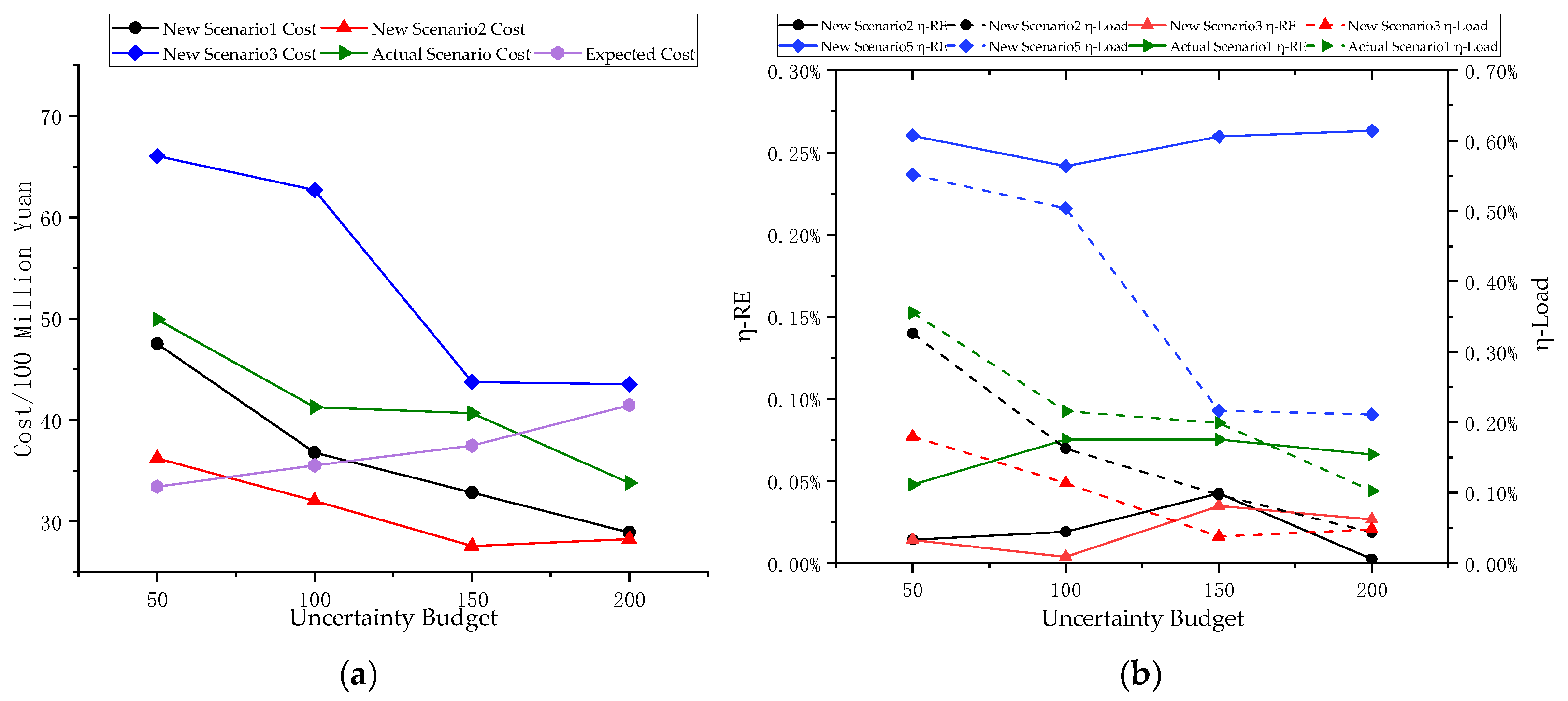
Taking four cases with uncertainty budgets of 50, 100, 150, and 200, respectively, carry out the proposed optimization method. Randomly select prediction errors, generate three new scenarios to verify the examples’ performance in different scenarios, which are, respectively, called New Scenario1, New Scenario2, and New Scenario3. The performance of the model in different scenarios was verified, and the results are shown in Figure 7. As the uncertainty budget increases, the expected cost gradually rises, while the actual operating cost gradually decreases. However, when the uncertainty budget increases to a certain value, the actual operating cost begins to recover slowly. As shown in the new scenario 2 in Figure 7a, when the uncertainty budget is set at 150, the actual operating cost is the smallest. When the uncertainty budget is set at 200, the cost is actually higher than when the uncertainty budget is set at 200.
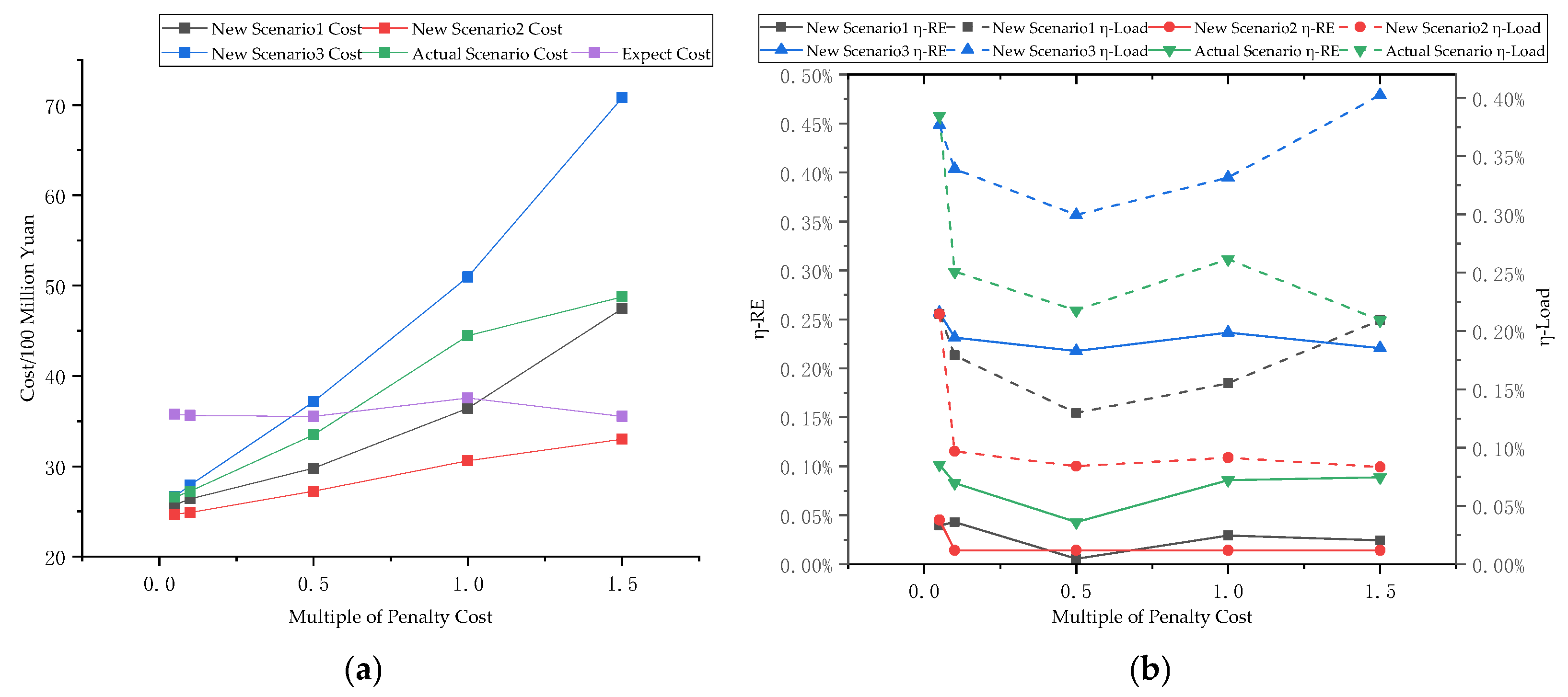
The penalty coefficients for renewable energy curtailment and load shedding are set to 0.05, 0.1, 0.5, and 1.5 times the values used in Section 4.1, respectively, and the results are presented in Figure 8. If the penalty coefficients for renewable energy curtailment and load shedding are less than a certain critical value, the load shedding rate and the renewable energy curtailment rate increase significantly. This is because the renewable energy curtailment and load shedding penalty costs are too small, and the model no longer takes avoiding renewable energy curtailment and load shedding as the optimization direction, resulting in a large amount of renewable energy power curtailment and load shedding in actual operation. When the penalty coefficients for renewable energy curtailment and load shedding exceed this critical value, avoiding renewable energy curtailment and load shedding remains the primary task of model optimization. No matter how much the penalty coefficients of renewable energy curtailment and load shedding increase, the rate of renewable energy curtailment and load shedding does not change much, but the actual operating cost increases rapidly.

5. Conclusions

To address the medium- and long-term optimal scheduling challenges for a renewable energy base comprising wind, solar, thermal power, and thermal storage, this study constructs a two-stage robust optimization model. The model explicitly accounts for both the thermal unit maintenance plan and the uncertainty of wind and photovoltaic output. In the first stage, the maintenance schedule and on/off plan of each unit are determined. In the second stage, the power output of every generation source is determined. A polyhedron set based on an uncertainty budget characterizes the fluctuations in wind and solar generation, and the overall problem is solved using the C&CG algorithm. Draw the following conclusions:
  • The proposed joint optimization framework realizes the collaborative decision-making of maintenance plans and operation scheduling, avoiding the problem of disconnection between maintenance arrangements and system regulation requirements in the traditional mode. Compared with the deterministic optimization, the proposed method reduces the load shedding rate by 0.6757%, and compared with the robust optimization with a pre-set maintenance plan, the proposed method reduces the load shedding rate by 0.1160%.
  • The case study analysis shows that in actual operation, compared with deterministic optimization, the load shedding rate of the proposed method is reduced by 0.6757%, and compared with the robust optimization with pre-set maintenance plans, the load shedding rate of the proposed method is reduced by 0.1160%.
  • The conservatism of the model is adjusted through the maximum fluctuation range and uncertainty budget. As the uncertainty budget and fluctuation range increase, the model’s conservatism rises, the expected cost increases, and the actual operating cost decreases. When the maximum fluctuation range is set at 0.6, the expected cost increases by 5.05447 billion yuan compared to when the maximum fluctuation range is set at 0.3, while the actual operating cost decreases by 1.57091 billion yuan.

Author Contributions

Conceptualization, L.J. and H.C.; methodology, M.X.; validation, L.J., M.X. and Q.X.; formal analysis, H.C.; resources, F.X.; data curation, L.C.; writing—original draft preparation, Q.X., L.H. and L.C.; writing—review and editing, L.J. and F.X.; visualization, J.L.; supervision, F.X.; project administration, L.H. All authors have read and agreed to the published version of the manuscript.

Funding

This research was funded by the project “Research and Application of Fully Domestic Secure Power Generation Control and Integrated Supervision System,” grant number CHDKJ24-04-01-35, and the project “Research and Application of Integrated Balance Regulation and Intelligent Decision-making for Source–Grid–Load–Storage under High-Penetration Renewable Energy,” grant number CHDKJ26-04-02-125.

Data Availability Statement

Data are available on request due to restrictions on privacy or ethics. The data presented in this study are available on request from the corresponding author.

Conflicts of Interest

Authors Ling Ji and Heng Chi were employed by Guodian Nanjing Automation Co., Ltd., Nanjing, China; authors Ling Ji, Heng Chi, Mingjun Xue and Qing Xu were employed by Nanjing SAC Power Grid Automation Co., Ltd., Nanjing, China. The remaining authors declare that the research was conducted in the absence of any commercial or financial relationships that could be construed as a potential conflict of interest. The authors declare that this study received funding from Guodian Nanjing Automation Co., Ltd. The funder was not involved in the study design, collection, analysis, interpretation of data, the writing of this article or the decision to submit it for publication.

References

  1. Wang, K.Y.; Zhu, H.T.; Dang, J.; Ming, B.; Wu, X. Short-term optimal scheduling of wind-photovoltaic-hydropower-thermal-pumped hydro storage coupled system based on a novel multi-objective priority stratification method. Energy 2024, 309, 133190. [Google Scholar] [CrossRef]
  2. Liu, H.T.; Zhai, R.R.; Patchigolla, K.; Turner, P.; Yu, X.H.; Wang, P. Multi-objective optimisation of a thermal-storage solar thermal power station-CSP-wind hybrid power system in three operation models. Energy 2023, 284, 129255. [Google Scholar] [CrossRef]
  3. Hu, B.J.; Cai, F.L.; Tai, N.L.; Wang, P. Dual-time scale optimal dispatch of the CSP-PV hybrid power plant considering dynamic operation. Energy 2024, 306, 132488. [Google Scholar] [CrossRef]
  4. Zhang, S.; Qiu, G.; Liu, Y.B.; Ding, L.J.; Shui, Y. Data-driven distributionally robust optimization-based coordinated dispatching for cascaded hydro-PV-PSH combined system. Electronics 2024, 13, 667. [Google Scholar] [CrossRef]
  5. Li, Y.G.; Su, Y.T.; Zhang, Y.J.; Wu, W.N.; Xia, L. Multiple-time-scale scheduling by optimizing the degradation cost models of hybrid energy storage systems in microgrids. Energy Convers. Manag. 2025, 343, 120186. [Google Scholar] [CrossRef]
  6. Dong, F.X.; Wang, J.J.; Xu, H.W.; Zhang, X.T. A robust real-time energy scheduling strategy of integrated energy system based on multi-step interval prediction of uncertainties. Energy 2024, 300, 131639. [Google Scholar] [CrossRef]
  7. Lu, X.H.; Li, H.B.; Zhou, K.L.; Yang, S.L. Optimal load dispatch of energy hub considering uncertainties of renewable energy and demand response. Energy 2023, 262, 125564. [Google Scholar] [CrossRef]
  8. Ye, Y.; Papadaskalopoulos, D.; Kazempour, J.; Strbac, G. Incorporating non-convex operating characteristics into bi-level optimization electricity market models. IEEE Trans. Power Syst. 2020, 35, 163–176. [Google Scholar] [CrossRef]
  9. Vahedipour-Dahraie, M.; Rashidizadeh-Kermani, H.; Anvari-Moghaddam, A. Risk-constrained stochastic scheduling of a grid-connected hybrid microgrid with variable wind power generation. Electronics 2019, 8, 577. [Google Scholar] [CrossRef]
  10. Okendo, E.O.; Farzaneh, H. A novel multi-objective bi-level optimization approach for strategic participation of hybrid renewable grid-connected microgrids in local electricity markets: Evidence from the Japan electric power exchange market. Appl. Energy 2026, 414, 127845. [Google Scholar] [CrossRef]
  11. Rodríguez, J.A.; Anjos, M.F.; Côté, P.; Desaulniers, G. MILP formulations for generator maintenance scheduling in hydropower systems. IEEE Trans. Power Syst. 2018, 33, 6171–6180. [Google Scholar] [CrossRef]
  12. Abiri-Jahromi, A.; Fotuhi-Firuzabad, M.; Parvania, M. Optimized Midterm Preventive Maintenance Outage Scheduling of Thermal Generating Units. IEEE Trans. Power Syst. 2012, 27, 1354–1365. [Google Scholar] [CrossRef]
  13. Amiri, S.; Honarvar, M.; Sadegheih, A. Providing an integrated model for planning and scheduling energy hubs and preventive maintenance. Energy 2018, 163, 1093–1114. [Google Scholar] [CrossRef]
  14. Helseth, A.; Fodstad, M.; Mo, B. Optimal hydropower maintenance scheduling in liberalized markets. IEEE Trans. Power Syst. 2018, 33, 6989–6998. [Google Scholar] [CrossRef]
  15. Wang, Y.; Kirschen, D.S.; Zhong, H.W.; Xia, Q.; Kang, C.Q. Coordination of generation maintenance scheduling in electricity markets. IEEE Trans. Power Syst. 2016, 31, 4565–4574. [Google Scholar] [CrossRef]
  16. Rokhforoz, P.; Gjorgiev, B.; Sansavini, G.; Fink, O. Multi-agent maintenance scheduling based on the coordination between central operator and decentralized producers in an electricity market. Reliab. Eng. Syst. Saf. 2021, 210, 107495. [Google Scholar] [CrossRef]
  17. Kang, K.; Su, Y.F.; Yang, P.; Wang, Z.J.; Liu, F. Securing long-term dispatch of isolated microgrids with high-penetration renewable generation: A controlled evolution-based framework. Appl. Energy 2025, 381, 125140. [Google Scholar] [CrossRef]
  18. Du, C.; Gao, Y.; Wang, L.; Li, X.; Cui, Y.; Gao, J. Medium- and Long-Term Optimal Stochastic Scheduling for Inter-Basin Hydro-Wind-Photovoltaic Complementary Systems Considering Wind and Solar Output Uncertainty. IEEE Open Access J. Power Energy 2025, 12, 404–416. [Google Scholar] [CrossRef]
  19. Lu, N.; Wang, G.Y.; Su, C.G.; Ren, Z.; Peng, X.; Sui, Q. Medium- and long-term interval optimal scheduling of cascade hydropower-photovoltaic complementary systems considering multiple uncertainties. Appl. Energy 2024, 353, 122085. [Google Scholar] [CrossRef]
  20. Liu, N.; Chen, Y.; Jiang, K.; Huang, J.; Wang, Z. Joint maintenance scheduling for generators and energy storage systems in sustainable power systems. Int. J. Electr. Power Energy Syst. 2026, 174, 111432. [Google Scholar] [CrossRef]
  21. Yang, X.; Zhao, Y.; Li, Y.; Huang, C.; Ding, Q. Generation Maintenance Scheduling for Power Systems Considering the Risk Quantification of Hybrid Uncertainty. IEEE Trans. Power Syst. 2025, 40, 3499–3512. [Google Scholar] [CrossRef]
  22. Liang, Z.; Yin, X.; Chung, C.Y.; Rayeem, S.K.; Chen, X.; Yang, H. Managing Massive RES Integration in Hybrid Microgrids: A Data-Driven Quad-Level Approach with Adjustable Conservativeness. IEEE Trans. Ind. Inform. 2025, 21, 7698–7709. [Google Scholar] [CrossRef]
  23. Qiu, D.; Zhang, S.; Luo, T.; Zhang, X. Global Sensitivity Analysis for Cyber-Physical Power Distribution Network. IEEE Trans. Ind. Cyber Phys. Syst. 2026, 4, 213–224. [Google Scholar] [CrossRef]
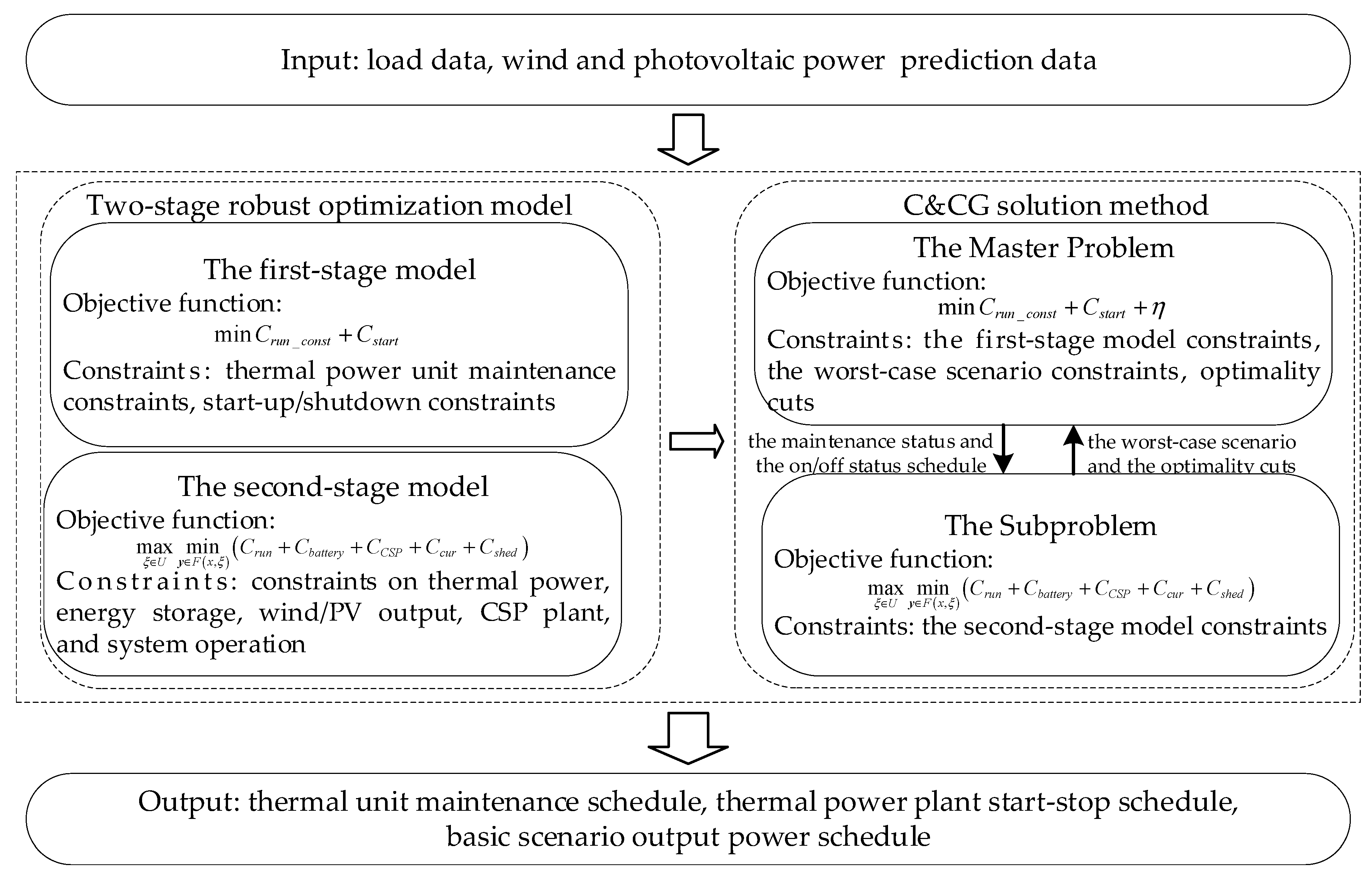
Figure 1. A robust optimization model framework considering the impacts of wind and photovoltaic output uncertainties and unit maintenance.
Electronics 15 02585 g001
Figure 2. C&CG algorithm solving process.
Electronics 15 02585 g002
Figure 3. Load, wind power, and PV power diagram in (a) load, forecast wind power, and actual wind power; (b) load, forecast PV power, and actual PV power.
Electronics 15 02585 g003
Figure 4. The convergence curve of the evaluated scenario.
Electronics 15 02585 g004
Figure 5. Comparison of the operation effects in terms of (a) cost, (b) renewable energy curtailment rate, and (c) load shedding rate.
Electronics 15 02585 g005aElectronics 15 02585 g005b
Figure 6. Generator maintenance schedule in (a) maintenance schedule of Scenario 1; (b) maintenance schedule of Scenario 2; (c) maintenance schedule of Scenario 3; (d) maintenance schedule of Scenario 4; (e) maintenance schedule of Scenario 5; (f) maintenance schedule of Scenario 6.
Electronics 15 02585 g006aElectronics 15 02585 g006b
Figure 7. Result comparison of different uncertainty budgets in (a) expected cost and actual cost; (b) renewable energy curtailment rate and load shedding rate. η-RE is the renewable energy curtailment rate, and η-Load is the load shedding rate.
Electronics 15 02585 g007
Figure 8. Results comparison of different renewable energy curtailment and load shedding penalty coefficients in (a) expected cost and actual cost; (b) renewable energy curtailment rate and load shedding rate. η-RE is the renewable energy curtailment rate, and η-Load is the load shedding rate.
Electronics 15 02585 g008
Disclaimer/Publisher’s Note: The statements, opinions and data contained in all publications are solely those of the individual author(s) and contributor(s) and not of MDPI and/or the editor(s). MDPI and/or the editor(s) disclaim responsibility for any injury to people or property resulting from any ideas, methods, instructions or products referred to in the content.