Embedded Implementation and Characterization of a Model Predictive Control in Velocity Form for Synchronous Motor Currents

Abstract

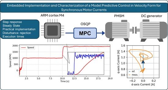
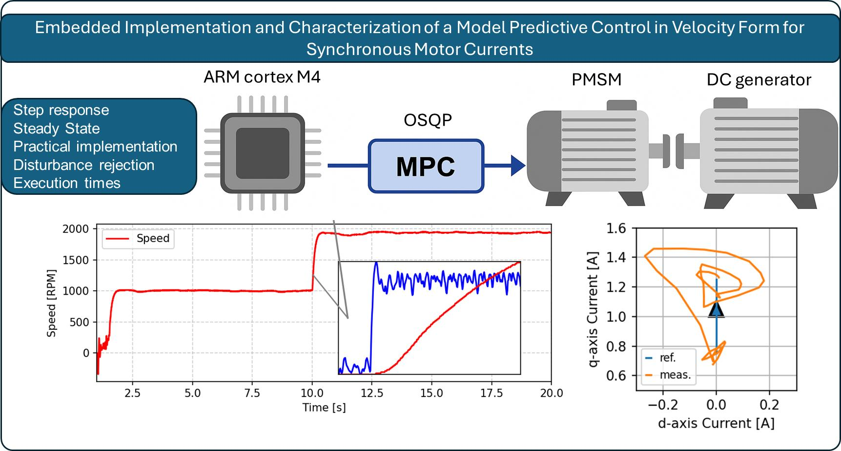
Electric motor control may be challenging due to nonlinearity, cross-coupling and current and voltage constraints. Multivariable action may enhance the effectiveness of control on electric motors. This work presents the real-time implementation of a Model Predictive Control (MPC) strategy for current regulation in a low-power synchronous electric motor, on a low-cost microcontroller platform. The experimental setup employs a back-to-back configuration with a DC motor operating as a generator, enabling comparative analysis of the impact of different cost-function formulations on the closed-loop dynamics. Both transient and steady-state capabilities have been investigated through suitable key performance indexes.

1. Introduction

The control of rotating electrical machines represents a crucial topic in modern drive applications, where efficiency, robustness, and high dynamic performance are increasingly demanded. The most common control architecture incorporates an outer loop for speed control and an inner loop for current control, most often of the Field Oriented Control (FOC) type. A conventional FOC routine makes use of Proportional Integral (PI) regulators, representing a valid industrial solution, but often with the hypothesis of perfectly independent action on d-axis and q-axis, that may be a rough approximation of the real condition of the machine. In fact, cross-coupling effects, magnetic saturation, thermal drift and other perturbations should not be neglected during control design [1].

To overcome the limitations of such single-input single-output control, several advanced control strategies have been proposed in the literature to enhance robustness and performance. Among them, sliding mode control approaches, such as super-twisting algorithms, as well as fractional-order control strategies for electrical drives, have been recently investigated, showing promising robustness properties [2,3]. On the other hand, Linear Quadratic Control (LQ) is of broad adoption thanks to its straightforward formulation within a solid theoretical framework and it is relevant for several applications, such as trajectory control for drones [4], microgrids [5], urban traffic networks [6] and motor control [7]. Even if robustness against disturbances can be built with Linear Quadratic Gaussian (LQG) control, by adding a stage of Kalman filtering for observing states [8], LQ control cannot explicitly incorporate operational constraints like voltage saturation or current limits for electric motors, and may therefore produce control actions that are theoretically optimal but actually infeasible.

The Model Predictive Control (MPC) has consequently emerged as a natural evolution, thanks to its ability to handle constraints directly into an optimization problem while predicting the future system behavior [9]. MPC is now widely adopted in electrical drives [10,11]. When applied to electrical machines, two main families of current MPC exist: the Continuous Control Set Model Predictive Control (CCS-MPC) and the Finite Control Set Model Predictive Control (FCS-MPC) [12]. Both rely on a discrete-time representation of the dynamical system. A FCS-MPC scheme evaluates candidate inverter switching states at each sampling step and selects the configuration that minimizes a cost function. This eliminates the need for modulation. Unless explicitly addressed [13], this approach may generate irregular switching patterns and non-uniform current spectra, which can result in undesirable noise or vibrations [14]. However, it is highly suitable for multi-level conversion [15] and for multi-objective cost functions [16]. On the other hand, the Continuous Control Set MPC requires an independent modulator, and it needs to solve a constrained optimization problem at each cycle.

Like LQ control, both CCS-MPC and FCS-MPC rely on an accurate dynamical model, assuming a perfect match between the prediction model and the actual system. Furthermore, MPC is usually applied to models of linear or linearized dynamics. Nonlinear MPC could relax this requirement at the cost of a higher computational burden, as it requires non-linear solvers [17,18].

An integral action is often added to improve robustness to model mismatch, enabling compensation of slowly varying disturbances while preserving the linear MPC framework. Within linear MPC with integral actions, for Continuous Control Set MPC, two main formulations are commonly adopted: disturbance-estimation MPC and velocity-form MPC [19]. The first augments the state with an explicit disturbance term and requires a dedicated estimation procedure, whereas the second directly controls increments of the input, inherently suppressing constant or slowly varying disturbances [20].

Due to limited computational resources, implementing MPC on microcontrollers is challenging. The optimization problem, typically expressed as a Quadratic Program (QP), must be solved at every control interval, requiring efficient numerical solvers and careful tuning to meet real-time constraints. Some works have demonstrated practical implementations for current control in synchronous machines. The main adopted solvers are OSQP (Operator Splitting Quadratic Programming) [21] and qpOASES (Quadratic Programming Online Active Set Strategy) [22]. In [23], a controller employs the qpOASES solver with an update frequency of 6 kHz and a prediction horizon of three steps, with a particular focus on constraint handling. Another implementation with qpOASES is in [19], with the comparison between the disturbance estimation approach and the velocity-form approach. However, both the cited studies rely on the use of Rapid Control Prototyping (RCP) units, with significantly greater computational capabilities than microcontrollers. Another study proposes an algorithm that guarantees convergence within a fixed computational window, ensuring deterministic performance on a low-cost platform [24].

This work presents an implementation of MPC with the OSQP solver on a low-cost platform, adopting a velocity-form MPC strategy, which avoids the additional estimation step, remains compatible with moderate model mismatch while compensating dominant disturbances. The paper is organized as follows: Section 2 introduces the main theoretical framework for the proposed controller, Section 3 describes the test setup, Section 4 collects the main steps of control design. In Section 5, the main results are presented.

2. Theoretical Framework

2.1. Dynamical Model

The equations of Kirchhoff Voltage Law (KVL) in the time domain, applied to a three-phase electric motor, can be represented as follows:

$$\begin{array}{c}\hfill \left\{\begin{array}{c}{v}_a=R_{ph}{i}_a+{\displaystyle \frac{d}{dt}}{\psi }_a\hfill \\ v_b=R_{ph}{i}_b+{\displaystyle \frac{d}{dt}}{\psi }_b\hfill \\ v_c=R_{ph}{i}_c+{\displaystyle \frac{d}{dt}}{\psi }_c\hfill \end{array}\right.\end{array}$$

(1)

where ${\psi }_{a,b,c}$ are the flux linkages, $R_{ph}$ is phase resistance, $v_{a,b,c}$ and $i_{a,b,c}$ are respectively phase voltages and currents. This set of equations can be represented on a suitable dq rotating reference frame by the mean of Clarke and Park transforms. The adopted amplitude invariant transformation matrix can be represented as follows:

$$\begin{array}{cc}\hfill {\mathbf{T}}_{dq}\left({\theta }_{el}\right)& ={\displaystyle \frac{2}{3}}\left[\begin{array}{ccc}cos\left({\theta }_{el}\right)& cos({\theta }_{el}-{\displaystyle \frac{2\pi }{3}})& cos({\theta }_{el}+{\displaystyle \frac{2\pi }{3}})\\ -sin\left({\theta }_{el}\right)& -sin({\theta }_{el}-{\displaystyle \frac{2\pi }{3}})& -sin({\theta }_{el}+{\displaystyle \frac{2\pi }{3}})\\ 1/2& 1/2& 1/2\end{array}\right]\hfill \end{array}$$

(2)

where ${\theta }_{el}$ is the electrical angular position of the rotor according to the reference choice. After the transformation, the resulting model of synchronous machines in the rotating $dq$ reference frame is described by the following compact set of differential equations:

$$\begin{array}{c}\hfill \left\{\begin{array}{c}{v}_d=R_s{i}_d+{\displaystyle \frac{d}{dt}}{\psi }_d-{\omega }_{el}{\psi }_q\hfill \\ v_q=R_s{i}_q+{\displaystyle \frac{d}{dt}}{\psi }_q+{\omega }_{el}{\psi }_d\hfill \end{array}\right.\\ \hfill T={\displaystyle \frac{3}{2}}p({\psi }_d{i}_q-{\psi }_q{i}_d)\end{array}$$

(3)

where $v_d$ and $v_q$ denote the stator voltages on the synchronous $dq$ frame, $i_d$ and $i_q$ represent the corresponding stator currents, $R_s$ is the equivalent stator phase resistance, and ${\psi }_d$ and ${\psi }_q$ are the flux linkages. The term ${\omega }_{\mathrm{el}}$ is the electrical angular velocity of the rotor, related to the mechanical angular velocity by ${\omega }_{\mathrm{el}}=p{\omega }_{\mathrm{r}}$, where p is the number of pole pairs. T is the generated torque. This formulation constitutes the standard basis for Field-Oriented Control [25] and it is adopted for the proposed control strategy.

Since fluxes are working point dependent, a single comprehensive state-space representation can not be built. When the system in (3) is referred to a Permanent Magnet Synchronous Motor (PMSM), a discrete-time state-space representation with fixed parameters can be constructed by grouping the electrical dynamics and introducing an additive disturbance term associated with the permanent-magnet flux. The continuous-time flux equations are written as follows:

$$\begin{array}{c}\hfill \left\{\begin{array}{ccc}\hfill \underset{\dot{\mathbf{x}}\left(t\right)}{\underbrace{{\displaystyle \frac{d}{dt}}\left[\begin{array}{c}{i}_d\\ i_q\end{array}\right]}}& =& \underset{\mathbf{A}}{\underbrace{\left[\begin{array}{c}-{\displaystyle \frac{R_s}{{\overline{L}}_d}}{\displaystyle \frac{{\overline{\omega }}_{el}{\overline{L}}_q}{{\overline{L}}_d}}\\ -{\displaystyle \frac{{\overline{\omega }}_{el}{\overline{L}}_d}{{\overline{L}}_q}}-{\displaystyle \frac{R_s}{{\overline{L}}_q}}\end{array}\right]}}\underset{\mathbf{x}\left(t\right)}{\underbrace{\left[\begin{array}{c}{i}_d\\ i_q\end{array}\right]}}+\underset{\mathbf{B}}{\underbrace{\left[\begin{array}{c}{\displaystyle \frac{1}{{\overline{L}}_d}}0\\ 0{\displaystyle \frac{1}{{\overline{L}}_q}}\end{array}\right]}}\underset{\mathbf{u}\left(t\right)}{\underbrace{\left[\begin{array}{c}{v}_d\\ v_q\end{array}\right]}}+\underset{\mathbf{M}}{\underbrace{\left[\begin{array}{c}0\\ -{\overline{\omega }}_{el}{\displaystyle \frac{{\varphi }_m}{{\overline{L}}_q}}\end{array}\right]}}\hfill \\ \hfill \underset{\mathbf{y}\left(t\right)}{\underbrace{\left[\begin{array}{c}{y}_1\\ y_2\end{array}\right]}}& =& \underset{\mathbf{C}}{\underbrace{\left[\begin{array}{cc}1& 0\\ 0& 1\end{array}\right]}}\left[\begin{array}{c}{i}_d\\ i_q\end{array}\right]\hfill \end{array}\right.\end{array}$$

(4)

where the inductances ${\overline{L}}_d$ and ${\overline{L}}_q$, as well as the speed ${\overline{\omega }}_{\mathrm{el}}$ are working-point specific, while ${\varphi }_m$ denotes the magnetic flux contribution of permanent magnets.

2.2. Velocity-Form MPC

Starting from the discrete-time state-space model of the PMSM in the $dq$ reference frame, the velocity-form representation is obtained by expressing the system in terms of state increments. The integral action of the velocity-form MPC allows to compensate for limited model mismatch, as shown in [19,20]. After Zero-Order Hold discretization with sampling time $T_s$, from which the matrices ${\mathbf{A}}_d$, ${\mathbf{B}}_d$, and ${\mathbf{C}}_d$ are obtained, the discrete-time model takes the form

$$\underset{{\epsilon }_{k+1}}{\underbrace{\left[\begin{array}{c}\delta {\mathbf{x}}_{k+1}\\ {\mathbf{e}}_{k+1}\end{array}\right]}}=\underset{{\overline{\mathbf{A}}}_d}{\underbrace{\left[\begin{array}{c}{\mathbf{A}}_{d}0\\ -{\mathbf{C}}_d{\mathbf{A}}_d\mathbf{I}\end{array}\right]}}\underset{{\epsilon }_k}{\underbrace{\left[\begin{array}{c}\delta {\mathbf{x}}_k\\ {\mathbf{e}}_k\end{array}\right]}}+\underset{{\overline{\mathbf{B}}}_d}{\underbrace{\left[\begin{array}{c}{\mathbf{B}}_d\\ -{\mathbf{C}}_d{\mathbf{B}}_d\end{array}\right]}}\delta {\mathbf{u}}_k$$

(5)

where the extended state vector can be defined as follows:

$${\epsilon }_k=\left[\begin{array}{c}\delta {\mathbf{x}}_k\\ {\mathbf{e}}_k\end{array}\right]=\left[\begin{array}{c}{\mathbf{i}}_{dq,k}-{\mathbf{i}}_{dq,k-1}\\ {\mathbf{i}}_{dq,k}^{ref}-{\mathbf{i}}_{dq,k}\end{array}\right]$$

(6)

Since the disturbance associated with the permanent magnet flux is proportional to rotor electrical speed, which is considered to be slowly varying with respect to the dynamics of the current loop, the following equation stands:

$${\omega }_{el,k}\approx {\omega }_{el,k-1}\Rightarrow {\mathbf{M}}_k-{\mathbf{M}}_{k-1}\approx 0.$$

(7)

causing the disturbance component to vanish from the incremental dynamics.

By defining $\mathbf{Q}$ as the state weighting matrix that penalizes deviations of the elements of the extended state vector, $\mathbf{R}$ as the input weighting matrix penalizing the increments in the control inputs and $\mathbf{S}$ as the terminal cost matrix, the proposed cost function can be represented as follows:

$$J={\displaystyle \sum _{i=0}^{N-1}}\left(\right||{\epsilon }_{k+i}{\left|\right|}_{\mathbf{Q}}^2+\left|\right|\delta {\mathbf{u}}_{k+i}{\left|\right|}_{\mathbf{R}}^2)+||{\epsilon }_{k+N}{\left|\right|}_{\mathbf{S}}^2$$

(8)

provided that $({\overline{\mathbf{A}}}_d,{\overline{\mathbf{B}}}_d)$ is reachable, $({\overline{\mathbf{A}}}_d,{\mathbf{Q}}^{1/2})$ is observable, $\mathbf{Q}={\mathbf{Q}}^T⪰0$, and $\mathbf{R}={\mathbf{R}}^T\succ 0$ with dimensions according to the system in (5). Operational constraints can be posed on $\delta {\mathbf{u}}_k$ and $\delta {\mathbf{x}}_k$. N is the number of steps of the prediction horizon. The terminal cost $\mathbf{S}$ is computed here as the solution of the Riccati equation of the unconstrained problem, which is a standard choice [26]. The choice of terminal cost and terminal set has implications on the stability of MPC [9], but it is not further considered. At each cycle, an optimal incremental control action $\delta {\mathbf{u}}_k$ is found and applied

$${\mathbf{u}}_k={\mathbf{u}}_{k-1}+\delta {\mathbf{u}}_k$$

(9)

2.3. Quadratic Programming Formulation for MPC

The velocity-form model enables the standard formulation of the Model Predictive Control, expressed as a QP problem of the form

$$\underset{\delta \mathbf{U}}{min}{\displaystyle \frac{1}{2}}\delta {\mathbf{U}}^{\prime }\mathbf{H}\delta \mathbf{U}+{\mathbf{f}}^{\prime }\delta \mathbf{U}$$

(10)

where

$$\delta \mathbf{U}=\left[\begin{array}{c}\delta {\mathbf{u}}_k\\ \delta {\mathbf{u}}_{k+1}\\ ⋮\\ \delta {\mathbf{u}}_{k+N-1}\end{array}\right]$$

(11)

The vector $\delta \mathbf{U}$ represents the control action from the instant k up to the instant k+N-1, but the applied control action is only the first step of the prediction ($\delta {\mathbf{u}}_k$). The optimization problem in (10) can be subject to eventual linear inequality constraints of the type

$$\mathbf{P}\delta \mathbf{U}\le \mathbf{b}$$

(12)

The matrix $\mathbf{P}$ defines the linear inequality constraints associated with voltage saturation and current limits, expressed either in absolute-value or incremental form. The vector $\mathbf{b}$ contains the corresponding admissible bounds, properly adjusted according to the current system state.

The optimization problem is formulated in a condensed form [27], where the Hessian matrix $\mathbf{H}$ and the inequality matrix $\mathbf{P}$ are pre-calculated offline and remain constant during the control routine, while the linear term $\mathbf{f}$ and the vector $\mathbf{b}$ are updated at each iteration according to the current operating conditions.

3. Test Equipment

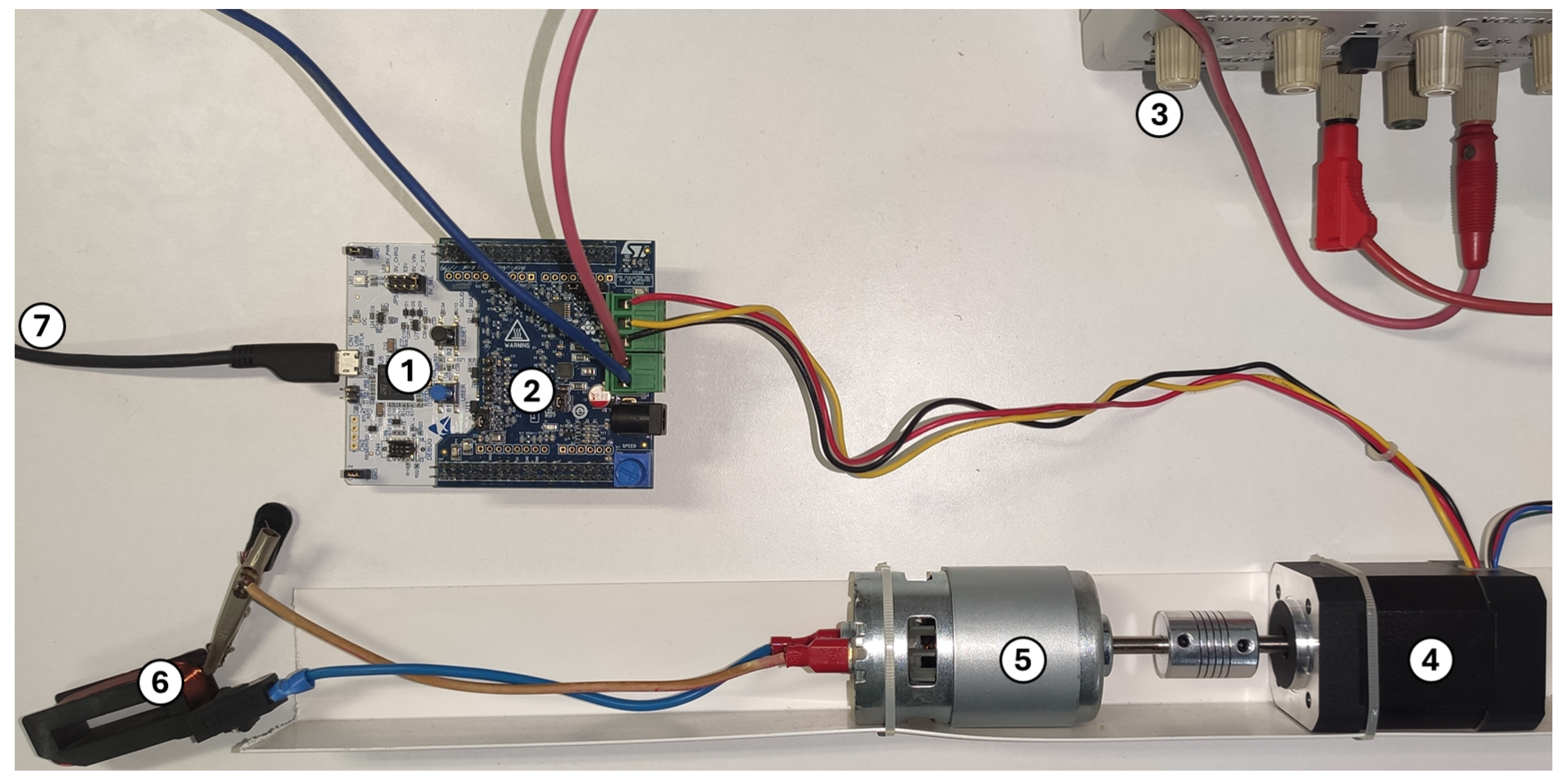
The proposed test setup is introduced here, and it is displayed in Figure 1.

3.1. Microcontroller and Power Stage

The control platform is built around the NUCLEO-G431RB development board with a STM32G431RB microcontroller (STMicroelectronics, Plan-les-Ouates, Geneva, Switzerland), equipped with a 32-bit Arm Cortex-M4 core with a single-precision floating-point unit and a clock frequency of 170 MHz. The family of STM32 microcontrollers is widely adopted for embedded applications in electric systems. Some applications can be found in battery storage systems [28], temperature estimation for permanent magnets in synchronous motors [29,30], performance enhancement of motors [31], advanced control techniques [32,33].

The power stage is implemented through the X-NUCLEO-IHM16M1 driver board (STMicroelectronics, Plan-les-Ouates, Geneva, Switzerland), provided with a low-power three-phase H-bridge. A three-shunt current-sensing architecture is employed. The driver board provides a back-electromotive force (BEMF) sensing circuit for sensorless operation. The system is powered by the model PS281 from Tektronix (Beaverton, Oregon, United States), a controlled DC power supply capable of delivering up to 30 V and 5 A. The main features of the selected microcontroller, power board and power supply are collected in

Table 1. Main characteristics of the driver board, power board and power supply.

Element	Model	Parameter	Value	Symbol
Microcontroller	STM32G431RB	Architecture	Arm Cortex-M4	–
		Clock frequency	170 MHz	$f_{ck}$
		Current sampling rate	153 MHz	$f_{sam}$
		Communication rate	3 kHz	$f_{com}$
		Current control ISR rate	3 kHz	$f_s$
Power stage	IHM16M1	Current sensing	Shunt resistors	–
		Max. DC input voltage	45 V	–
		Maximum current	2 A	–
		Maximum continuous power	40 W	–
		Switching frequency	15 kHz	$f_{sw}$
Power supply	PS281	Maximum voltage	30 V	–
		Maximum current	5 A	–

. The selected operating DC voltage is 24 V.

3.2. Communication and Measurements

The rotor position and the mechanical speed are estimated with a sensorless method based on BEMF observation. The communication interface between the control board and the computer is implemented via a USART peripheral, configured at a baud rate of 1,843,200 bps. The USB connection simultaneously supplies the logic stage with 5 V and provides a port for serial communication. Phase currents are measured with the shunt resistors integrated in the driver stage, with a maximum measurable current of ±3.3 A and a resolution of 32,767 counts. The accuracy of the measurement chain is not addressed in this work, but the measured signals are considered sufficiently accurate for comparative evaluation of the various control strategies. The recorded quantities are: voltages and currents in the $dq$ reference frame, measured currents in the $\alpha \beta$ framework, current setpoints and estimated speed.

3.3. Electric Motor

The controlled machine is a three-phase PMSM with surface-mounted permanent magnets (SPM), a unit of DT4260-24-055-04H-TI from TelcoMotion (Houston, TX, USA), of the NEMA standard 17. The main parameters are collected in

Table 2. Motor parameters.

Name	Symbol	Value
Pole pairs	p	4
Line–line resistance	$R_{LL}$	0.8 $\mathrm{\Omega }$
Nominal voltage	$V_{DC}$	24 V
No-load speed	$n_0$	6000 rpm
Nominal torque	$T_n$	125 mNm
Nominal speed	$n_n$	4000 rpm
Peak torque	$T_{peak}$	380 mNm
Torque constant	$k_T$	35.5 mNm/A
Voltage constant	$k_e$	2.71 V/krpm
Rotor inertia	I	48 g·cm2
Weight	m	0.45 kg
Height	H	42 mm
Width	W	42 mm
Depth	D	60.3 mm

. The motor was profiled using an automatic tuning procedure, and the resulting parameters are used as the basis of the control strategies adopted in the present work. The equivalent phase resistance at ambient temperature is $R_s=0.5$ $\mathrm{\Omega }$. The estimated d-axis inductance is ${\overline{L}}_d=0.28\mathrm{mH}$. This value has been obtained using a standard identification procedure, based on the injection of a voltage signal along the d-axis and the subsequent estimation of the motor parameters from the resulting current response. The dynamical model in (4) has been built around a speed of 1000 rpm. For the negligible saliency, it is assumed ${\overline{L}}_d\approx {\overline{L}}_q$. The motor torque is therefore generated only by the q-axis current.

3.4. Mechanical Load

The motor shaft is mechanically coupled through an elastic coupling to a separately excited, brushed DC motor of the commercial RS-775 type, with a voltage constant $k_{E,DC}=$ 11.5 mV/(rad/s). The DC motor operates as a generator and provides a speed-dependent load torque. The electrical load is implemented using an external 0.8 $\mathrm{\Omega }$ series resistor. With the hypothesis of limited thermal drift and negligible friction, the torque is given by

$$T_{DC}={\displaystyle \frac{k_{E,DC}^2{\omega }_r}{R}}$$

(13)

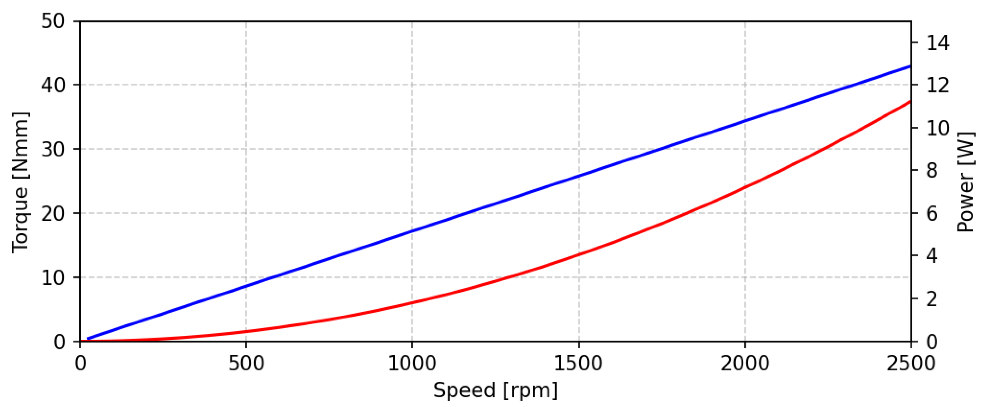
where R represents the sum of load resistance and armature resistance and ${\omega }_r$ is the mechanical speed of the rotor, expressed in rad/s. The analytically estimated curve is represented in Figure 2.

4. Control

4.1. Cost Functions

Since the cost function is quadratic, the optimal solution of the QP problem remains unchanged as long as the relative scaling among the cost weights is preserved. However, the condition number of the Hessian matrix $\mathbf{H}$, and therefore the robustness and the speed of convergence, is strongly influenced by relative magnitudes of the cost weight in a non-trivial way. Typically, weighting matrices are chosen in diagonal form, assigning independent penalties to each state or input. However, the effect of the variation of an individual element of the weighting matrix is difficult to isolate in the resulting control action, leading to a case-dependent and generally non-intuitive tuning process. For these reasons, the impact of the weight elements has been studied by varying the cost matrices to implement different cost functions.

The considered weight matrices and the condition numbers for the resulting matrices $\mathbf{H}$ are collected in

Table 3. Definition of controllers through cost functions.

Label	Q	R	cond(H) *
C1	diag(0.1 ${\lambda }_x$, 0.1 ${\lambda }_x$, ${\lambda }_x$, ${\lambda }_x$) **	diag(100${\lambda }_u$, $100{\lambda }_u$)	12.1
C2	diag(0.1 ${\lambda }_x$, 0.1 ${\lambda }_x$,$10{\lambda }_x$, $10{\lambda }_x$)	diag($100{\lambda }_u$, $100{\lambda }_u$)	39.7
C3	diag(0.1 ${\lambda }_x$, 0.1 ${\lambda }_x$,${\lambda }_x$, ${\lambda }_x$)	diag($1000{\lambda }_u$, $1000{\lambda }_u$)	3.5

* cond(H) represents the condition number of the Hessian matrix, ** diag(·) represents the diagonal matrix with the displayed elements.

. The selection of the weighting factors was carried out based on a normalization approach. By considering representative values for the states and inputs ($\overline{x}=1\mathrm{A}$, $\overline{u}=10\mathrm{V}$, the following normalized weights were obtained:

$$\left\{\begin{array}{c}{\lambda }_x={\displaystyle \frac{1}{{\overline{x}}^2}}=1\hfill \\ {\lambda }_u={\displaystyle \frac{1}{{\overline{u}}^2}}=0.01\hfill \end{array}\right.$$

(14)

Furthermore, due to the isotropic nature of the machine, identical weights were assigned along both the d-axis and the q-axis. Three different cost functions have been analyzed. For the first cost function, hereafter labeled as controller 1 (C1), a baseline configuration is considered: the elements of $\mathbf{Q}$ associated with current increments are weighted less ($0.1{\lambda }_x$), while the remaining states, associated with errors, are weighted with ${\lambda }_x$. The input weighting matrix $\mathbf{R}$ is set to $100{\lambda }_u$, providing a balanced trade-off between tracking performance and control effort. For the second cost function (C2), the weights associated with errors are increased to $10{\lambda }_x$, while keeping $\mathbf{R}$ unchanged. This configuration emphasizes the reduction of specific state errors, resulting in a more aggressive response that may lead to faster but potentially more oscillatory dynamics. Finally, for controller 3 (C3), the state weighting matrix $\mathbf{Q}$ is kept identical to C1, while the input weighting matrix $\mathbf{R}$ is increased to $1000{\lambda }_u$. This choice strongly penalizes the control action, leading to a smoother response at the expense of slower dynamics. In all cases, the weights associated with the increments are kept low to preserve a satisfactory dynamic response.

4.2. Settings for Real-Time Operation

The choice of the prediction horizon is $N=3$. The controller is refreshed at 3 kHz. For an immediate reference, the motor has a time constant of ${\tau }_{el}={\overline{L}}_d/R_s$ = 0.56 ms, whereas the prediction horizon covers $N/f_s=1$ ms. The refresh frequency of the controller may be unsuitably low as the switching frequency. Therefore, the switching frequency has been set to 15 kHz, and the controller is called every 5 PWM cycles.

A warm-start procedure is employed. At each cycle, the initial guess for the QP solution is initialized using the solution from the previous time step

$$\delta {\mathbf{U}}_k^{\left(0\right)}=\delta {\mathbf{U}}_{k-1}$$

(15)

where $\delta {\mathbf{U}}_k^{\left(0\right)}$ denotes the first guess of the solution at the instant k. When consecutive optimal solutions do not differ significantly, warm starting can drastically reduce the necessary number of iterations for convergence. A maximum of four solver iterations per cycle was found empirically through successive experimental trials. The value is comparable with what has been found in [24] for the implementation of MPC on microcontrollers.

The absolute and relative tolerances are set to 1% and 0.1% respectively. If the solver fails, the control increments are set to zero; whereas, if the solver finds an inaccurate solution, the control update is still applied. Although these settings may occasionally produce a suboptimal response, they reduce the computational burden, increasing operational robustness by prioritizing continuity over strict optimality. Constraints are imposed only on the immediate next prediction step, as extending them over the full prediction horizon may excessively restrict the feasibility region or increase solving time.

The modulation technique is Space Vector Modulation (SVM). The maximum allowable amplitude for voltage will be referred to as $U_M$, whereas the maximum allowable current is defined as $I_M$. The constraints on voltages must ensure

$$\left|\right|{\mathbf{u}}_{k-1}+\delta {\mathbf{u}}_k\left|\right|<U_M$$

(16)

which prevents the incremental action from exceeding the available voltage margin. At each instant, such an amplitude constraint expands into four scalar inequalities, corresponding to the maximum and minimum admissible values of the d and q axis voltage components. On the other hand, current constraints can be imposed according to

$$\left|\right|{\mathbf{x}}_k+{\mathbf{A}}_d\delta {\mathbf{x}}_k+{\mathbf{B}}_d\delta {\mathbf{u}}_k\left|\right|<I_M$$

(17)

from which four other scalar inequalities can be built. The dimensions of the matrices are the following: ${\mathbf{H}}^{6\times 6}$, ${\mathbf{Q}}^{4\times 4}$, ${\mathbf{R}}^{2\times 2}$, ${\mathbf{S}}^{4\times 4}$, ${\mathbf{P}}^{8\times 6}$, ${\mathbf{b}}^{8\times 1}$, $\delta {\mathbf{U}}^{6\times 1}$, and $\delta {\mathbf{u}}_k^{2\times 1}$.

5. Results

5.1. Mission Profile

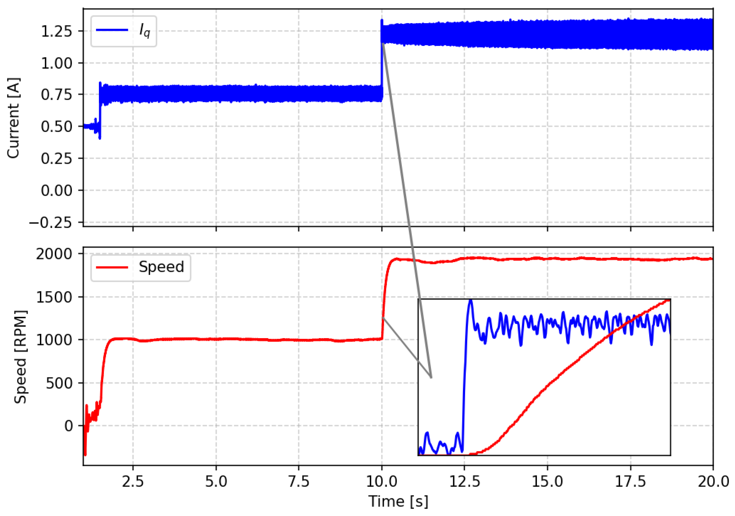
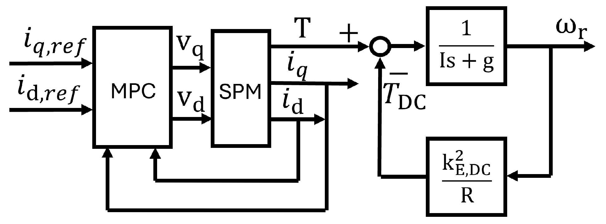
The system is driven in torque control mode. As a result, the speed is a torque-dependent output, according to the mechanical dynamics and the DC motor characteristic curve from Figure 2. The functional block scheme of the proposed setup is illustrated in Figure 3, where I denotes the rotational inertia of the system and g denotes the friction coefficient for the transfer function for the mechanical block in the Laplace-domain notation. From idle, the motor is gradually driven to a first target of 0.75 A of q-axis current, with a resulting speed of around 1000 rpm. Then, a step of amplitude 0.5 A is imposed to reach a 1.25 A q-axis current setpoint, with a resulting speed of around 1930 rpm. Then, 10 s of steady-state operation are acquired. The procedure is repeated for all the proposed controllers in Table 3. The whole mission profile for one of the recorded acquisitions is displayed in Figure 4. The zoomed detail highlights that the electrical subsystem reaches steady state prior to any significant mechanical response. The startup procedure is carried out with open-loop operation until the speed crosses a 200 rpm threshold, beyond which the virtual speed sensor is considered sufficiently reliable.

5.2. Transient Characterization

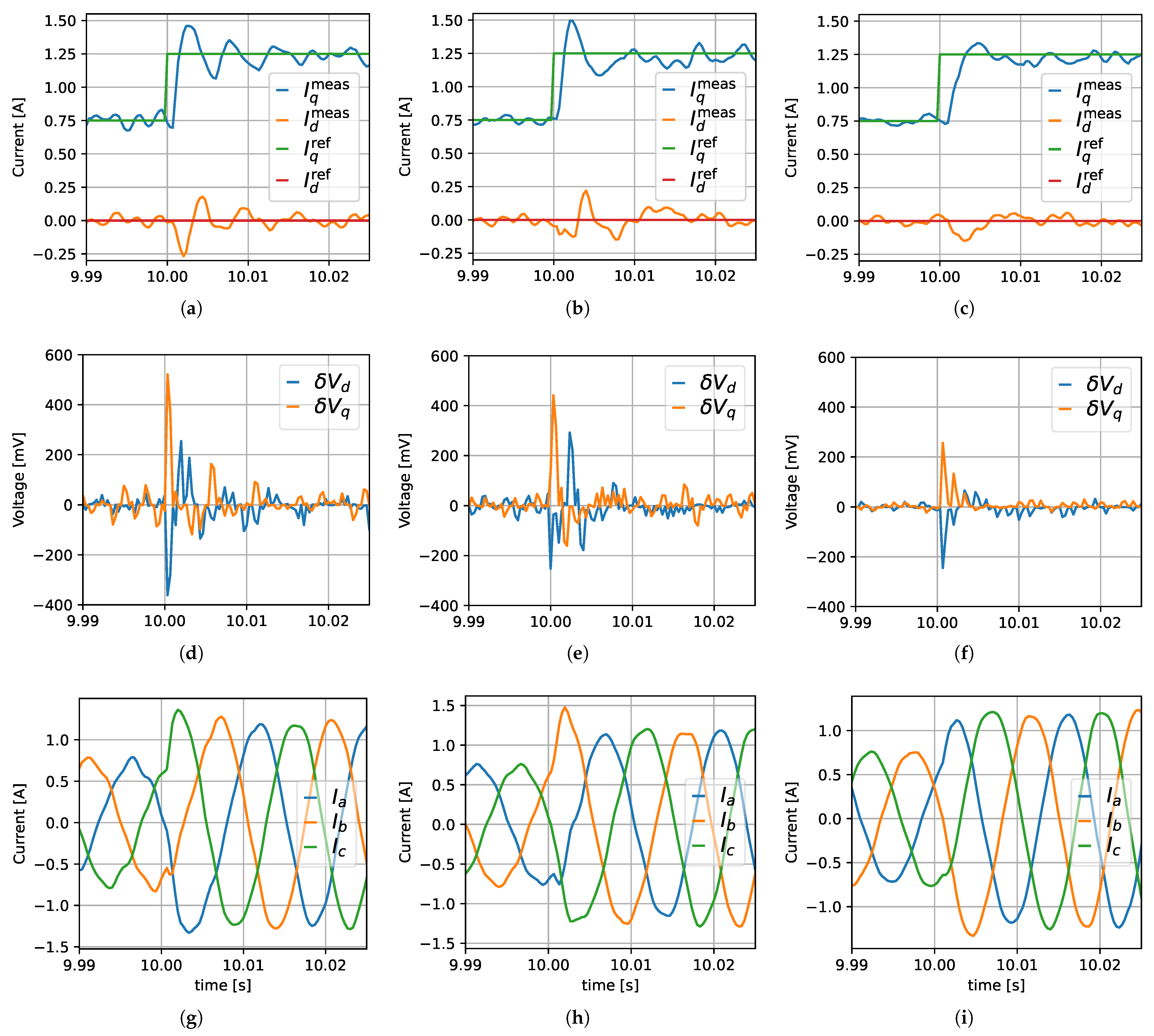
The transient performance of the proposed controller is assessed by analyzing the current and voltage waveforms around the instant at which the step is applied. In Figure 5, the curves of the currents and the underlying control actions are illustrated for all the considered controllers. For C3, due to the higher weighting applied to the elements of the matrix $\mathbf{R}$, which penalizes the control effort, a slower response is observed, as shown in Figure 5c. This behavior is consistent with the intentionally less aggressive control action when compared with C1, in Figure 5a and C2, in Figure 5b, whose responses exhibit similar settling times. The maximum peak ($M_p$) overshoot for q-axis current is defined as follows:

$$M_p={\displaystyle \frac{\max \left(i_{q,k}\right)-i_{q,ref}}{i_{q,ref}}}$$

(18)

The maximum recorded value of 31.7% is observed for C1, a value of 35.0 % is recorded for C2 and a sensibly lower value of 20.5 % is observed for C3. The maximum magnitude of the control increment vector is defined as follows:

$$\delta u_{\max }=\max \parallel \delta u_k\parallel$$

(19)

The amplitudes are equal to 64 mV for C1, as in Figure 5d, 44 mV for C2, as shown in Figure 5e and the minimum value of 36 mV is recorded for C3, shown in Figure 5f, respecting the smoother control approach of the relative cost function. Currents in the $abc$ reference frame are represented in Figure 5g for C1, in Figure 5h for C2 and in Figure 5i for C3.

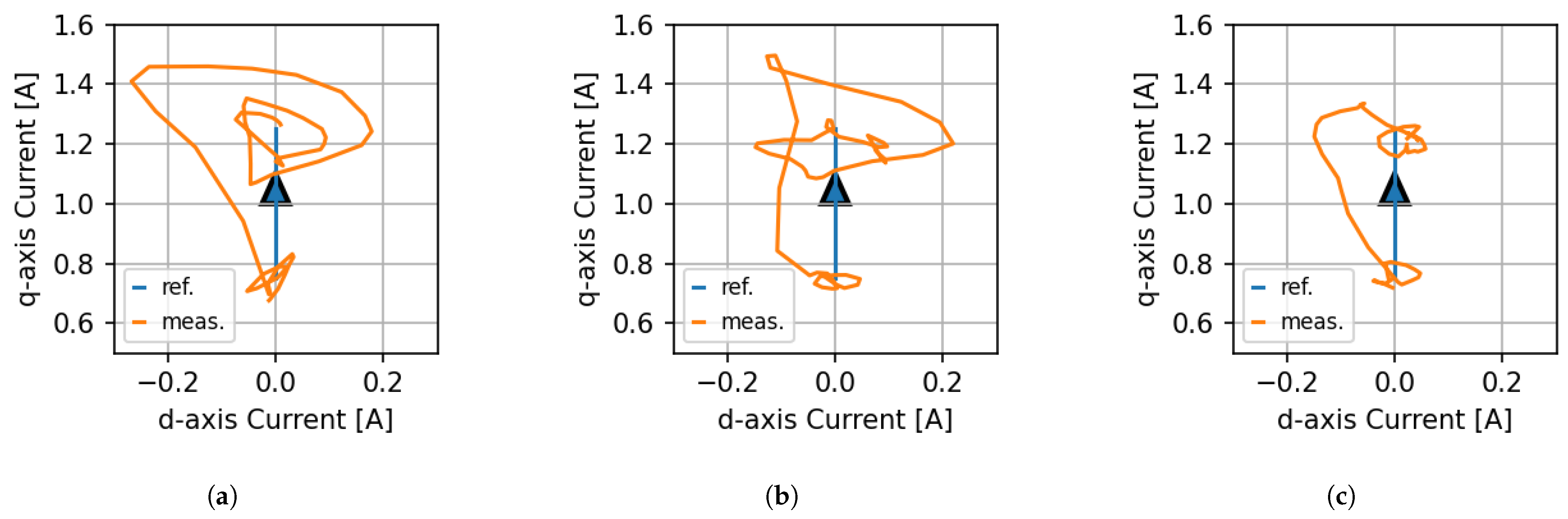
The trajectories of the current vector in the $dq$ plane during the transient are shown for the three cases in Figure 6. As expected, the trajectory corresponding to C3, in Figure 6c, exhibits a reduced deviation from the reference path, which can be considered an additional indicator of a less aggressive control policy. The trajectory of C2 shows in Figure 6b some sharp corners, which are not present for the other cases. This may be due to the high penalty assigned to the error, which may lead to a faster-acting response by design.

5.3. Execution Time Measurement

The execution times ($t_{exec}$) of the proposed routine have been measured by the means of the DWT (Data Watchpoint and Trace). Maximum execution time and mean execution time have been recorded along the mission profile in Figure 4. The execution time for the whole ISR (Interrupt Service Routine) has been separated from the execution time of the QP problem solving, including the update of the linear vector and the update of constraints. The results are collected in

Table 4. Execution times for ISR and QP problem solving.

Label	ISR Mean ${\mathit{t}}_{\mathit{exec}}$ [$\mathsf{\mu }$s]	ISR Worst ${\mathit{t}}_{\mathit{exec}}$ [$\mathsf{\mu }$s]	QP Mean ${\mathit{t}}_{\mathit{exec}}$ [$\mathsf{\mu }$s]	QP Worst ${\mathit{t}}_{\mathit{exec}}$ [$\mathsf{\mu }$s]
C1	249	296	234	286
C2	255	297	240	286
C3	250	295	234	286

. All the controllers exhibit similar execution times. As a result, the employed OSQP solver appears to be largely insensitive to the condition number of the Hessian matrix within the tested range, although issues may arise for significantly higher condition numbers.

5.4. Steady-State Characterization

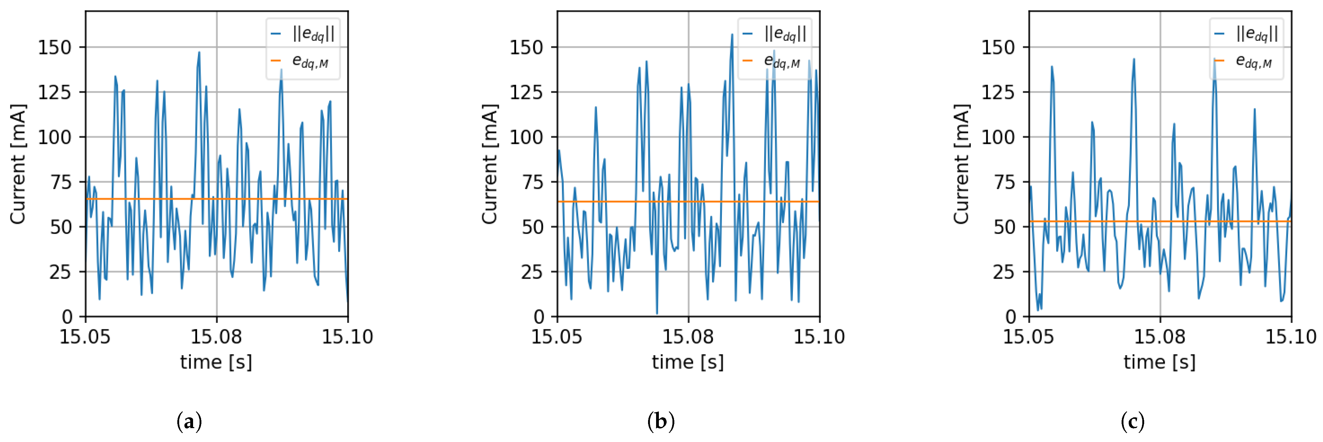
The proposed mission profile captures 10 s of steady-state regulation to study the steady-state performance of the controllers. Since the MPC used in this work behaves as a linear regulator, any harmonic components are propagated through the feedback loop. Each controller provides a distinct level of attenuation of the propagated harmonic content. The harmonic content of the currents is predominantly composed of low-frequency components, which originate from spatial harmonics of the machine. The most immediate parameter to consider is the mean amplitude of the error vector during the steady-state condition. It is always non-zero due to intrinsic oscillation from the feedback signal. However, a lower value implies a better steady-state regulation of the state. This quantity can be defined as follows, along a window of $N_w$ samples

$${\mathrm{e}}_{dq,M}={\displaystyle \frac{1}{N_w}}{\displaystyle \sum _{k=1}^{N_w}}\sqrt{e_d^2\left[k\right]+e_q^2\left[k\right]}={\displaystyle \frac{1}{N_w}}{\displaystyle \sum _{k=1}^{N_w}}\sqrt{{\left(i_{d,\mathrm{ref}}\left[k\right]-i_d\left[k\right]\right)}^2+{\left(i_{q,\mathrm{ref}}\left[k\right]-i_q\left[k\right]\right)}^2}$$

(20)

For the considered controllers, the quantity is illustrated in Figure 7. For C1 and C2, the quantity is comparable, with the values of 65 mA and 64 mA respectively. C3 leads to the best steady-state regulation with 52 mA.

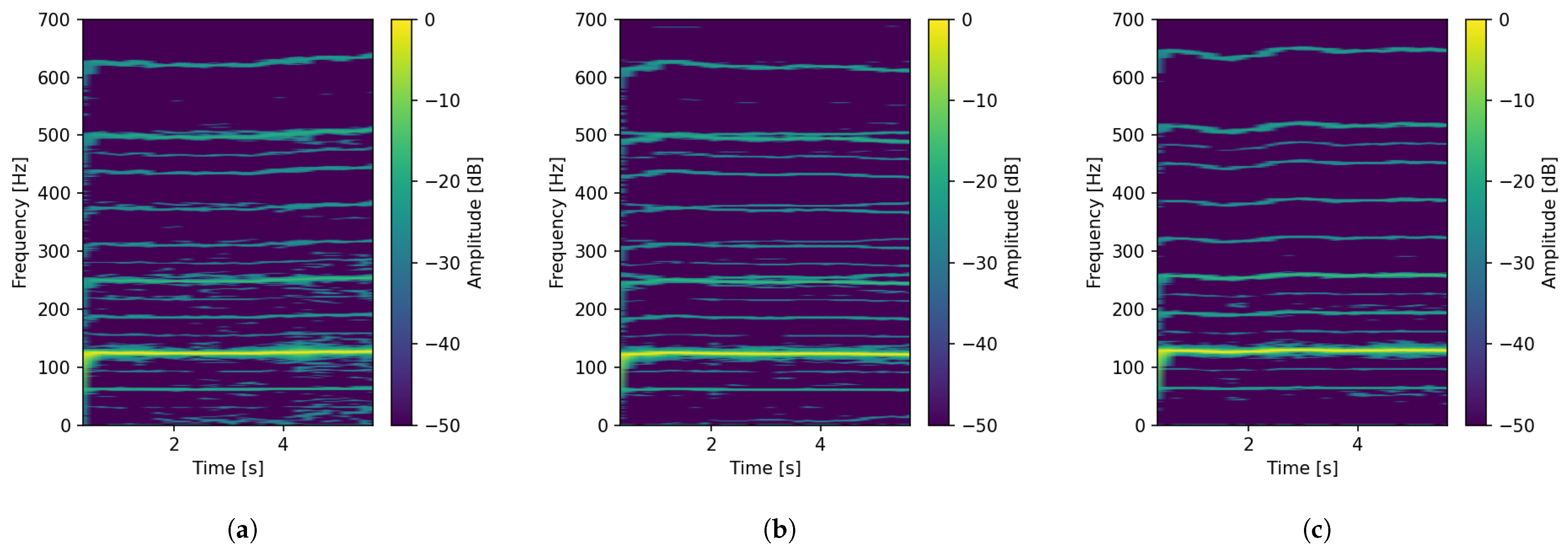
Steady-state behaviour has also been investigated in the frequency domain, with a study performed on the acquired currents. Figure 4 shows some time variability of the acquired speed. Generally, for closed-loop systems applied to synchronous electrical drives, the application of a Fast Fourier Transform (FFT) on the signals may be inadequate due to the variability of the fundamental frequency, which is directly proportional to speed. To carry out frequency analysis on signals with slow time-varying fundamental frequency, some advanced techniques exist, such as Short Time Fourier Transform (STFT) [34] or Dragon transform [35,36]. For the proposed study, the STFT has been considered. A richer spectrum in harmonics is a possible indicator of subpar regulation for steady-state operation. The spectrograms are calculated with the application of a 2048 points FFT, with a 75% of overlapping, after the application of a window of the Hann type and then normalized. Measurement data are acquired with the same update frequency as the current controller, leading to a Nyquist frequency of 1500 Hz, with the 11th harmonic as the highest observable order for the considered working point.

The resulting spectrograms for the acquired steady-state operation are illustrated in Figure 8. The oscillation of the fundamental frequency is visible for each of the proposed representations. However, the spectrograms for C1 and C2 reveal richer harmonic content, indicating a less effective filtering action of the controllers, aligned with the faster response due to a higher penalty for the error. The proposed index to evaluate the steady-state behaviour in the frequency domain has been designed as follows:

$${\mathrm{E}}_{\%}:={\displaystyle \frac{E-E_1}{E}}$$

(21)

where $E_1$ is the energy associated with the fundamental frequency $f_1$, whereas E is the total energy of the signal, calculated from the spectrogram $\mathbf{X}(f,t)$

$$\begin{array}{c}\hfill E_1=\sum _{f_1}\sum _t\mathbf{X}{(f,t)}^2\\ \hfill E=\sum _f\sum _t\mathbf{X}{(f,t)}^2\end{array}$$

(22)

For C1, a value of 58.1% is recorded. For C2, 55.0%, whereas C3 has the lower value with 34.4%.

5.5. Load Disturbance Analysis

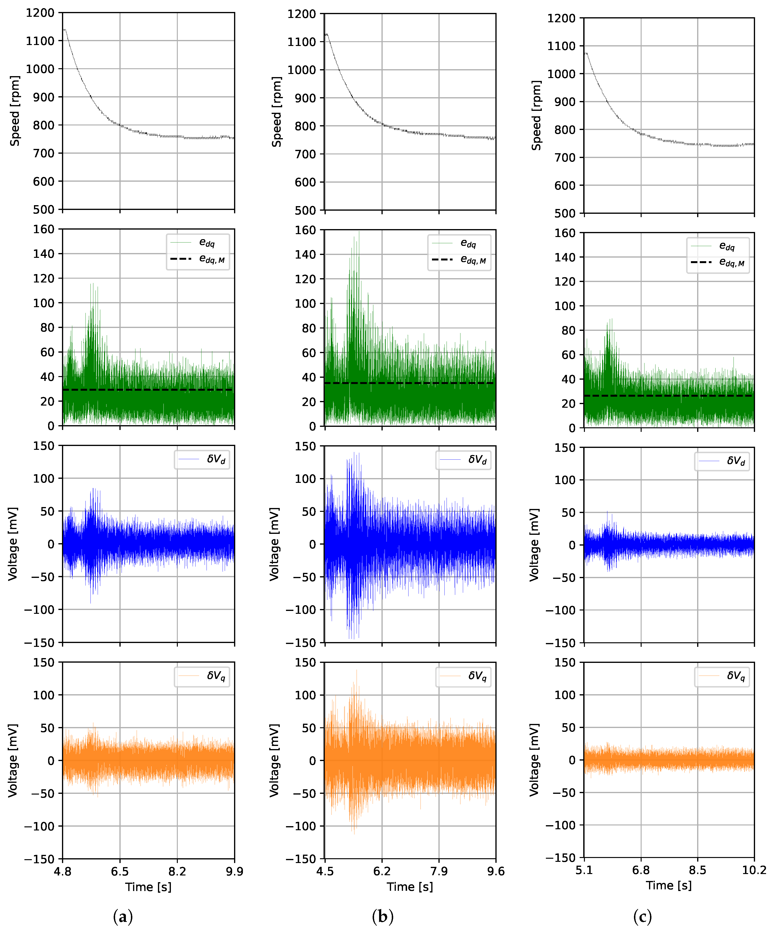
To evaluate the robustness against load variations, experimental tests were performed at a fixed current setpoint. A reference value of 0.35 A for the q-axis current was selected, and the transition from no-load conditions to the connection of a 10 $\mathrm{\Omega }$ load resistor was recorded. The corresponding results are shown in Figure 9.

During the transient, the rotor speed decreases due to the applied load, and all controllers exhibit noticeable oscillations. The observed behavior is consistent with the step-response characteristics: C3 provides the smoothest control action, achieving the lowest mean error ($e_{dq,M}=26$ mA) and the smallest peak error (90 mA). In contrast, C2 shows the most aggressive behavior, with the highest control variation ($\delta u_{\max }=194$ mV) and larger tracking errors ($e_{dq,M}=35$ mA, with a maximum value of 159 mA). A complete comparison is reported in

Table 5. Numerical results for load disturbance rejection.

Label	$\mathit{\delta }{\mathit{u}}_{\mathit{max}}$ [mV]	$\mathit{max}\left({\mathit{e}}_{\mathit{dq}}\right)$ [mA]	${\mathit{e}}_{\mathit{dq},\mathit{M}}$ [mA]
C1	93	116	29
C2	194	159	35
C3	52	90	26

.

6. Conclusions

This work presented the embedded implementation of a velocity-form Model Predictive Control for current regulation in a low-power PMSM. The controller was executed in real time on a low-cost platform using a condensed QP formulation and the OSQP solver with a limited number of iterations.

Experimental validation on a back-to-back test bench confirmed that different cost–function configurations have a direct impact on the control performances. Controllers with lower input penalization achieved faster transients, whereas a stronger penalization of the control action resulted in improved steady-state behavior and reduced harmonic content.

The results highlight the trade-off between dynamical response and steady-state operation, and show that velocity-form MPC may represent an alternative to conventional regulators when multivariable interactions and constraints must be accounted for. Future work may address computational optimization for horizon extension, analysis of recursive feasibility, and further testing on different synchronous motors, such as Synchronous Reluctance motors, Interior Permanent Magnet motors, and Wound Field Synchronous Machines. The behaviour around the maximum performance curve, to test constraints handling, will also be investigated. A structured comparison with a state-of-the-art PI controller will be performed.

References

1. Busarello, T.D.C.; Bubshait, A.; Varaprasad, O.V.S.R.; Alsaleem, A.; Simões, M.G. A Comprehensive Methodology of Field-Oriented Control Design with Parameter Variation Analysis for Interior Permanent Magnet Synchronous Machine Drives. IEEE Access 2025, 13, 89524–89541. [Google Scholar] [CrossRef] [Scilit]
2. Tuyen, T.T.; Yang, J.; Liao, L.; Thao, N.G.M. Recent Advances in Sliding Mode Control Techniques for Permanent Magnet Synchronous Motor Drives. Electronics 2025, 14, 3933. [Google Scholar] [CrossRef] [Scilit]
3. Hou, Q.; Ding, S.; Yu, X.; Mei, K. A Super-Twisting-Like Fractional Controller for SPMSM Drive System. IEEE Trans. Ind. Electron. 2022, 69, 9376–9384. [Google Scholar] [CrossRef] [Scilit]
4. Martins, L.; Cardeira, C.; Oliveira, P. Linear Quadratic Regulator for Trajectory Tracking of a Quadrotor. IFAC-PapersOnLine 2019, 52, 176–181. [Google Scholar] [CrossRef] [Scilit]
5. Patarroyo-Patarroyo-Montenegro, J.F.; Andrade, F.; Guerrero, J.M.; Vasquez, J.C. A Linear Quadratic Regulator with Optimal Reference Tracking for Three-Phase Inverter-Based Islanded Microgrids. IEEE Trans. Power Electron. 2020, 36, 7112–7122. [Google Scholar] [CrossRef] [Scilit]
6. Wang, H.; Zhu, M.; Hong, W.; Wang, C.; Tao, G.; Wang, Y. Optimizing Signal Timing Control for Large Urban Traffic Networks Using an Adaptive Linear Quadratic Regulator Control Strategy. IEEE Trans. Intell. Transp. Syst. 2020, 23, 333–343. [Google Scholar] [CrossRef] [Scilit]
7. Shi, T.; Yan, Y.; Zhou, Z.; Xiao, M.; Xia, C. Linear Quadratic Regulator Control for PMSM Drive Systems Using Nonlinear Disturbance Observer. IEEE Trans. Power Electron. 2019, 35, 5093–5101. [Google Scholar] [CrossRef] [Scilit]
8. Liu, H.; Hu, F.; Su, J.; Wei, X.; Qin, R. Comparisons on Kalman-Filter-Based Dynamic State Estimation Algorithms of Power Systems. IEEE Access 2020, 8, 51035–51043. [Google Scholar] [CrossRef] [Scilit]
9. Li, N.; Chen, H.; Li, M.; Yu, S.; Huang, Y. Model Predictive Control: Past, Present, and Future. Control Theory Technol. 2026, 24, 173–193. [Google Scholar] [CrossRef] [Scilit]
10. Rodriguez, J.; Garcia, C.; Mora, A.; Flores-Bahamonde, F.; Acuna, P.; Novak, M.; Zhang, Y.; Tarisciotti, L.; Davari, S.A.; Zhang, Z.; et al. Latest Advances of Model Predictive Control in Electrical Drives—Part I: Basic Concepts and Advanced Strategies. IEEE Trans. Power Electron. 2022, 37, 3927–3942. [Google Scholar] [CrossRef] [Scilit]
11. Rodriguez, J.; Garcia, C.; Mora, A.; Davari, S.A.; Rodas, J.; Valencia, D.F.; Elmorshedy, M.; Wang, F.; Zuo, K.; Tarisciotti, L.; et al. Latest Advances of Model Predictive Control in Electrical Drives—Part II: Applications and Benchmarking with Classical Control Methods. IEEE Trans. Power Electron. 2022, 37, 5047–5061. [Google Scholar] [CrossRef] [Scilit]
12. Yu, Z.; Long, J. Review on Advanced Model Predictive Control Technologies for High-Power Converters and Industrial Drives. Electronics 2024, 13, 4969. [Google Scholar] [CrossRef] [Scilit]
13. Aguirre, M.; Kouro, S.; Rojas, C.A.; Rodriguez, J.; Leon, J.I. Switching Frequency Regulation for FCS-MPC Based on a Period Control Approach. IEEE Trans. Ind. Electron. 2018, 65, 5764–5773. [Google Scholar] [CrossRef] [Scilit]
14. Li, T.; Sun, X.; Lei, G.; Guo, Y.; Yang, Z.; Zhu, J. Finite-Control-Set Model Predictive Control of Permanent Magnet Synchronous Motor Drive Systems—An Overview. IEEE/CAA J. Autom. Sin. 2022, 9, 2087–2105. [Google Scholar] [CrossRef] [Scilit]
15. Gemma, F.; Tresca, G.; Riccio, J.; Mohammadzadeh, B.; Volpini, A.; Zanchetta, P. Computationally Efficient MPC with Embedded Adaptive Battery Balancing for CHB Inverters. IEEE Trans. Ind. Appl. 2026, 1–10. [Google Scholar] [CrossRef] [Scilit]
16. Gemma, F.; Riccio, J.; Rovere, L.; Tresca, G.; Volpini, A.; Zanchetta, P. Model-Predictive Control of Open-End Winding Synchronous Reluctance Motor Drives. IEEE Trans. Ind. Appl. 2026, 1–10. [Google Scholar] [CrossRef] [Scilit]
17. Santos, J.C.; Gouttefarde, M.; Chemori, A. A Nonlinear Model Predictive Control for the Position Tracking of Cable-Driven Parallel Robots. IEEE Trans. Robot. 2022, 38, 2597–2616. [Google Scholar] [CrossRef] [Scilit]
18. Zhang, H.; Prempain, E. A Non-Linear Offset-Free Model Predictive Control Design Approach. Actuators 2024, 13, 322. [Google Scholar] [CrossRef] [Scilit]
19. Favato, A.; Carlet, P.G.; Toso, F.; Torchio, R.; Bolognani, S. Integral Model Predictive Current Control for Synchronous Motor Drives. IEEE Trans. Power Electron. 2021, 36, 13293–13303. [Google Scholar] [CrossRef] [Scilit]
20. Schimperna, I.; Rubino, A.; Magni, L. Velocity Form MPC for Current Control in Synchronous Reluctance Motors. IEEE Trans. Control Syst. Technol. 2025, 33, 2463–2469. [Google Scholar] [CrossRef] [Scilit]
21. Stellato, B.; Banjac, G.; Goulart, P.; Bemporad, A.; Boyd, S. OSQP: An Operator Splitting Solver for Quadratic Programs. Math. Program. Comput. 2020, 12, 637–672. [Google Scholar] [CrossRef] [Scilit]
22. Ferreau, H.J.; Kirches, C.; Potschka, A.; Bock, H.G.; Diehl, M. QpOASES: A Parametric Active-Set Algorithm for Quadratic Programming. Math. Program. Comput. 2014, 6, 327–363. [Google Scholar] [CrossRef] [Scilit]
23. Toso, F.; Carlet, P.G.; Favato, A.; Bolognani, S. On-line Continuous Control Set MPC for PMSM Drives Current Loops at High Sampling Rate Using qpOASES. In Proceedings of the 2019 IEEE Energy Conversion Congress and Exposition (ECCE), Baltimore, MD, USA, 29 September–3 October 2019; pp. 6615–6620. [Google Scholar] [CrossRef] [Scilit]
24. Cimini, G.; Bernardini, D.; Levijoki, S.; Bemporad, A. Embedded Model Predictive Control with Certified Real-Time Optimization for Synchronous Motors. IEEE Trans. Control Syst. Technol. 2020, 29, 893–900. [Google Scholar] [CrossRef] [Scilit]
25. De Boni, G.; Mantione, L.; Minervini, M.; Frosini, L. Look-Up Table Based Reduced Order Model of Synchronous Motors for Digital Twin Applications. 2025 IEEE Workshop on Electrical Machines Design, Control and Diagnosis (WEMDCD), Valletta, Malta, 9–10 April 2025; pp. 1–6. [Google Scholar] [CrossRef] [Scilit]
26. Ahuar, R.L.; Figueroa, D.; Agüero, J.C.; Silva, C.A. Experimental Validation of Offset-Free Model-Based Predictive Control in Voltage Source Inverters for Grid Connected and Microgrids Applications. Appl. Sci. 2025, 15, 1567. [Google Scholar] [CrossRef] [Scilit]
27. Jerez, J.L.; Kerrigan, E.C.; Constantinides, G.A. A sparse and condensed QP formulation for predictive control of LTI systems. Automatica 2012, 48, 999–1002. [Google Scholar] [CrossRef] [Scilit]
28. Barros, A.; Peretti, E.; Fabroni, D.; Carrera, D.; Fragneto, P.; Boracchi, G. Adaptive Extended Kalman Filtering for Battery State of Charge Estimation on STM32. IEEE Embed. Syst. Lett. 2025, 17, 160–163. [Google Scholar] [CrossRef] [Scilit]
29. Liao, X.; Chen, S.; Long, Y.; Zhao, S. Neural Dynamics Model for Temperature Estimation of Permanent Magnet Synchronous Motor. IEEE Trans. Veh. Technol. 2025, 74, 11993–12003. [Google Scholar] [CrossRef] [Scilit]
30. Czerwinski, D.; Gęca, J.; Kolano, K. Machine Learning for Sensorless Temperature Estimation of a BLDC Motor. Sensors 2021, 21, 4655. [Google Scholar] [CrossRef] [Scilit]
31. Antony, R.P.; Komarasamy, P.R.G.; Ibrahim, M.A.; Alanazi, A.; Rajamanickam, N. Performance Enhancement of Wireless BLDC Motor Using Adaptive Reinforcement Learning for Sustainable Pumping Applications. Sustainability 2025, 17, 10881. [Google Scholar] [CrossRef] [Scilit]
32. Kroičs, K.; Būmanis, A. BLDC Motor Speed Control with Digital Adaptive PID-Fuzzy Controller and Reduced Harmonic Content. Energies 2024, 17, 1311. [Google Scholar] [CrossRef] [Scilit]
33. Zhang, P.; Shi, Z.; Yu, B.; Qi, H. Research on the Control Method of a Brushless DC Motor Based on Second-Order Active Disturbance Rejection Control. Machines 2024, 12, 244. [Google Scholar] [CrossRef] [Scilit]
34. De Boni, G.; Fernandez-Cavero, V.; Frosini, L.; Duque-Perez, O.; Morinigo-Sotelo, D. Fault Harmonics Current Detection in Closed-Loop Controlled Induction Motors. In Proceedings of the 2023 IEEE 14th International Symposium on Diagnostics for Electrical Machines, Power Electronics and Drives (SDEMPED), Chania, Greece, 22–25 August 2023; pp. 443–449. [Google Scholar] [CrossRef] [Scilit]
35. Mantione, L.; Garcia-Calva, T.; Fernandez-Cavero, V.; Frosini, L.; Moriñigo-Sotelo, D. Broken Rotor Bar Detection in Closed Loop Inverter Fed Induction Motors Through Time-Frequency Techniques. IEEE Trans. Ind. Appl. 2025, 61, 209–217. [Google Scholar] [CrossRef] [Scilit]
36. Bonet-Jara, J.; Fernandez-Cavero, V.; Vedreno-Santos, F.; Morinigo-Sotelo, D.; Pons-Llinares, J. Very Accurate Time-Frequency Representation of Induction Motors Harmonics for Fault Diagnosis Under Load Variations. IEEE Trans. Ind. Appl. 2024, 60, 3903–3911. [Google Scholar] [CrossRef] [Scilit]
Figure 1. Test setup: microcontroller board (1), driver board (2), DC supply (3), PMSM motor (4), DC generator (5), load resistor (6), and USB communication (7).
Electronics 15 02561 g001
Figure 2. Analytically estimated mechanical load characteristics as a function of rotational speed: load torque (red) and load power (blue).
Electronics 15 02561 g002
Figure 3. Block scheme of the realized control.
Electronics 15 02561 g003
Figure 4. Mission profile with zoom box on the studied step reference change.
Electronics 15 02561 g004
Figure 5. Current step characterization. d q currents: C1 (a), C2 (b), and C3 (c). Control actions: C1 (d), C2 (e), and C3 (f). Currents in a b c framework: C1 (g), C2 (h), and C3 (i).
Electronics 15 02561 g005
Figure 6. d q plane trajectories for measured currents and setpoints during transient: C1 (a), C2 (b), and C3 (c).
Electronics 15 02561 g006
Figure 7. Steady-state error amplitude: C1 (a), C2 (b), and C3 (c).
Electronics 15 02561 g007
Figure 8. Spectrogram for steady-state operation: C1 (a), C2 (b), and C3 (c).
Electronics 15 02561 g008
Figure 9. Load disturbance rejection: C1 (a), C2 (b), and C3 (c).
Electronics 15 02561 g009