Article

Connectivity Assessment: Strength, Trend, and Regularity in Opportunistic Networks


by
William C. da Rosa
1,*,
Celso B. Carvalho
1,*,
Marcel W. R. da Silva
2,
Raphael M. Guedes
3,
André C. Mendes
4 and
Waldir S. S. Junior
1
1
Faculty of Electrical and Computer Engineering, Federal University of Amazonas, 6200 Gen. Rodrigo Octavio Ave., Coroado, Manaus 69080-900, AM, Brazil
2
Department of Computer Science, Federal Rural University of Rio de Janeiro, Gov. Roberto Silveira Ave., Moquetá, Nova Iguaçu 26285-060, RJ, Brazil
3
Department of Informatics and Computer Science, Rio de Janeiro State University, 524 São Francisco Xavier St, Maracanã, Rio de Janeiro 20550-900, RJ, Brazil
4
VALORIZA—Research Centre for Endogenous Resource Valorization, Portalegre Polytechnic University, Campus Politécnico, 7300-555 Portalegre, Portugal
*
Authors to whom correspondence should be addressed.
Electronics 2026, 15(11), 2351; https://doi.org/10.3390/electronics15112351
Submission received: 29 April 2026 / Revised: 23 May 2026 / Accepted: 26 May 2026 / Published: 28 May 2026

Highlights

What are the main findings?
  • The proposed CASTRO protocol utilizes connectivity strength, trend, and regularity to achieve delivery rates near 90% in both dense pedestrian and sparse vehicular networks.
  • Integrating Q-Learning (QL-CASTRO) reduces average delivery latency while maintaining high delivery rates and moderate overhead.
What are the implications of the main findings?
  • Combining socially aware metrics with reinforcement learning offers a robust, autonomous alternative to flooding-based routing in resource-constrained IoT environments.
  • Dynamic delay estimation and message retirement policies effectively prevent buffer saturation without requiring end-to-end connectivity or global topology knowledge.

Abstract

Routing in Opportunistic Networks (OppNets) is continuously challenged by intermittent connectivity and severe resource constraints. To address these limitations, this paper proposes CASTRO, a novel routing architecture, alongside its reinforcement learning extension, QL-CASTRO. The primary novelty lies in the mathematical modeling of disconnection intervals (OFF-mode) to extract precise social indicators—Strength, Trend, and Regularity—providing a robust alternative to traditional encounter-frequency metrics. To overcome the latency penalties inherent to conservative social routing, QL-CASTRO integrates a tabular Q-Learning paradigm. This acts as a dynamic acceleration mechanism, fusing social metrics with autonomous delivery delay estimates and strict message retirement policies. Performance was rigorously evaluated using the ONE simulator across dense pedestrian (Helsinki) and sparse vehicular (Manaus) environments. The results demonstrate that both protocols achieve high delivery rates near 90%. Crucially, QL-CASTRO significantly reduces average delivery latency compared to the baseline CASTRO protocol while maintaining moderate overhead and low energy consumption. Ultimately, this hybrid approach offers a scalable, resource-efficient routing solution for dynamic IoT environments where system longevity and information integrity are paramount.

1. Introduction

The technological evolution of embedded systems and the ubiquity of mobile devices have fundamentally expanded the scope of the Internet of Things (IoT) [1,2,3,4]. Beyond traditional data dissemination, modern opportunistic architectures provide the essential transport layer for Edge Intelligence (EI), where the confluence of machine learning and edge computing enhances system responsiveness and data privacy in infrastructure-less environments [5]. These decentralized networks are increasingly vital for emerging paradigms, such as federated digital twin construction via distributed sensing [6]. In these complex frameworks, synchronization between physical assets and virtual replicas must overcome dynamic topologies and edge-cloud collaboration challenges, making the freshness of status updates—conceptualized as the Age of Information (AoI)—critical for system fidelity [7].
To sustain data dissemination amidst stochastic connectivity, Opportunistic Networks (OppNets)—a specialized subset of Delay/Disruption-Tolerant Networks (DTNs) [8,9]—rely on the physical movement of nodes. Establishing continuous end-to-end communication links is often unfeasible in highly dynamic environments. Such operational scenarios include unmanned aerial vehicles (UAVs) [10,11], vehicular ad hoc networks (VANETs) [12,13,14], wildlife monitoring [15], agriculture [16], and maritime search operations [17], among others. Therefore, nodes perform decentralized communication via the store-carry-forward paradigm. The core routing dilemma consists of formulating autonomous forwarding decisions that maximize the probability of message delivery while strictly minimizing latency and the depletion of constrained resources. Consequently, efficient buffer management [18,19,20,21] and the mitigation of rapid battery exhaustion caused by continuous beaconing and data transmission [22,23,24,25] are paramount to ensure network sustainability.
Historically, routing algorithms have attempted to balance this operational trade-off through various taxonomic approaches [26,27]. Pure flooding mechanisms, exemplified by the Epidemic protocol [28], achieve optimal delivery rates under ideal conditions but rapidly induce network congestion. To mitigate such overhead, controlled replication frameworks like Spray and Wait (SnW) [29,30] restrict the upper limit of message copies, an approach continuously refined by recent stable transmission capacity evaluations [31]. Bridging these extremes, history-based probabilistic architectures—notably PRoPHET [32] and several derived approaches [33,34,35,36,37,38]—utilize past encounter frequencies and transitivity to estimate future delivery predictability.
Recent advancements have transitioned towards utility-based and hybrid routing strategies. These models extract sophisticated social metrics [39], influential node characteristics [40], node centrality [41], and relational trees [42] to evaluate reliability. Frameworks such as HESnW [43] incorporate multiple predictability metrics, while QoN-ASW [44] assesses the Quality of Node by merging message handling capacity with predictability functions. Despite these theoretical refinements, an analytical gap persists. Most contemporary algorithms prioritize data from periods when nodes are actively connected (ON-mode) [44]. While recent efforts have begun to explore connection separation times (OFF-mode) to improve probabilistic routing [45], these approaches typically rely on heuristic exponential decays and trajectory similarities as auxiliary parameters to extend traditional protocols like PRoPHET. Consequently, they lack a formal mathematical bounding of the OFF-mode temporal distribution. To accurately predict future encounters without inducing heavy computational overhead, it is imperative to model the statistical variance of inter-contact times against a proven theoretical limit, providing a deterministic assessment of social regularity among nodes.
To address the limitations of rigid heuristic rules, researchers have increasingly adopted Reinforcement Learning (RL) and Markov Decision Processes (MDP) to optimize routing in dynamic networks [46,47,48,49,50]. Recent high-quality works, such as the distributed DDPG-based resource allocation model proposed by Zheng et al. [7], demonstrate the power of deep reinforcement learning (DRL) in minimizing AoI in mobile IoT environments. However, applying RL specifically to OppNet routing presents unique challenges. While existing RL-based OppNet protocols show great potential, they often encounter practical challenges. They can struggle with state-space scalability and generally depend on frequent contacts to converge, which limits their effectiveness in sparse mobility scenarios where reward feedback is delayed. Furthermore, although Deep RL (DRL) approaches are highly capable, they require memory footprints and tensor operations that often stretch the sub-megabyte static RAM limits of autonomous edge devices [51,52]. As a result, these intensive computational models typically depend on edge-server offloading [53]—a condition that is difficult to ensure in the infrastructure-less nature of OppNets.
Motivated by the need for a routing protocol that balances data reliability with IoT hardware constraints, this paper introduces CASTRO—a novel routing architecture for Connectivity Assessment based on Strength, Trend, and Regularity in Opportunistic networks—alongside its reinforcement learning extension, QL-CASTRO.
QL-CASTRO addresses the modern demands of edge frameworks by utilizing social metrics to support the reliable propagation of data in Federated Learning environments, where heterogeneous devices operate as autonomous intelligent agents [54]. QL-CASTRO operates as a hybrid mechanism, relying on the mathematical evaluation of the OFF-mode to establish a robust social baseline. This social intelligence effectively guides the exploration space, allowing a bounded, tabular Q-Learning agent to achieve more stable convergence even in sparse environments. This design strategically accepts a modest O(N) memory footprint, focusing on dynamic delivery delay estimation and proactive message retirement to filter out stale data.
The main contributions of this paper are summarized as follows:
  • Analytical Modeling of the OFF-Mode: We propose the CASTRO protocol, which extracts precise social indicators (Strength, Trend, and Regularity) strictly from encounter history, providing a robust mathematical foundation to evaluate node consistency.
  • Dynamic Delay Estimation via Tabular Q-Learning: We introduce QL-CASTRO, which integrates a lightweight Q-Learning paradigm to balance the strictly conservative nature of social routing. Rather than pursuing absolute lowest latency at the cost of network flooding, this extension couples social metrics with autonomous delay estimation to reduce the latency of the CASTRO protocol.
  • TTL Rejuvenation and Message Retirement: We implement dynamic TTL (Time-To-Live) renewal alongside strict message retirement policies. By extending the lifespan of messages traversing reliable paths and actively filtering out stale data, this mechanism prevents premature buffer drops and channel saturation. Ultimately, this acts as the primary driver for achieving the high delivery success rates that characterize both the CASTRO and QL-CASTRO protocols.
  • Rigorous Empirical Validation: Extensive simulations in both dense pedestrian (Helsinki) and sparse vehicular (Manaus) environments demonstrate that both protocols achieve delivery rates near 90%, significantly outperforming contemporary baselines in delivery rates with low energy consumption.
The remainder of this article is organized as follows. Section 2 delineates the mathematical formulation of the connectivity metrics and introduces both the CASTRO protocol and its Q-Learning-based extension, alongside the experimental configuration. Section 3 presents the simulation results in dense pedestrian and sparse vehicular environments. Section 4 provides a comprehensive discussion of the performance outcomes. Finally, Section 5 concludes the study.

2. Materials and Methods

To effectively navigate the unpredictable topology of OppNets, the proposed routing architecture relies on a rigorous evaluation of historical contact patterns. Rather than simply counting encounter frequencies, the framework models both the connection and disconnection phases of the nodes. This section details the mathematical formulation of the connectivity metrics, the design of the CASTRO and QL-CASTRO protocols, and the experimental configuration used for performance validation.

2.1. System Model and Social Connectivity Metrics

In a highly dynamic network, the interaction history between any pair of mobile nodes, i and j , can be segmented into discrete temporal intervals. When the nodes are within transmission range and establish a valid communication link, they operate in an active state (ON-mode). Conversely, the absence of a link designates an inactive state (OFF-mode). The cumulative duration of all active intervals is denoted as t O N , whereas the sum of all inactive intervals is defined as t O F F .
To illustrate these concepts, Figure 1 depicts a hypothetical encounter history for node i interacting with nodes j and k within a specific time window ( t = 300 s), highlighting their connection intervals. As shown in Figure 1, nodes i and j established six brief connection intervals (10 s each). Meanwhile, nodes i and k established two longer intervals (30 s each).
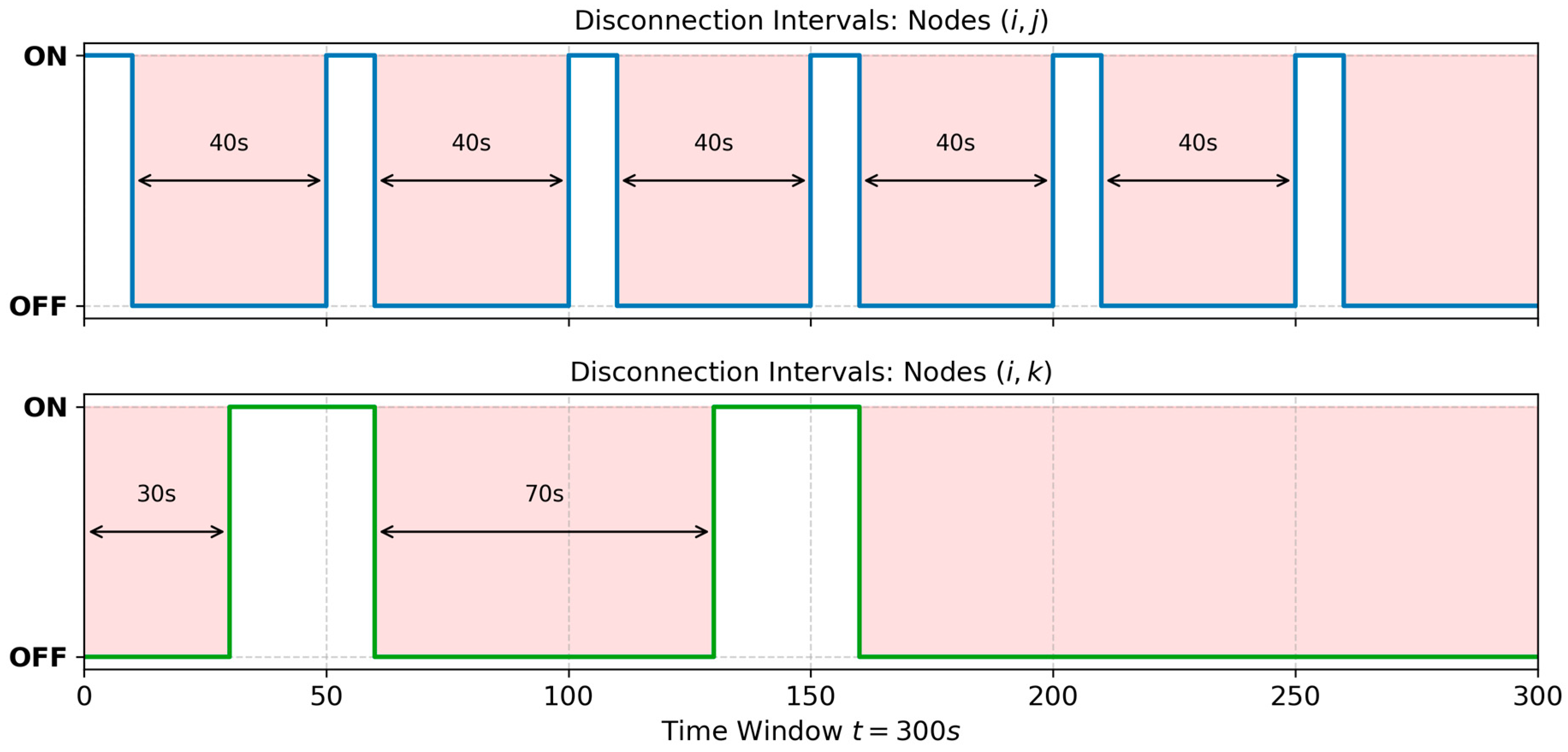
Concurrently, Figure 2 illustrates the corresponding disconnection intervals for the same scenario. Figure 2 reveals their disconnection patterns. Nodes i and j experienced six uniform disconnection intervals (40 s each). Nodes i and k recorded two distinct intervals (30 s and 70 s). Note that the final ongoing period of inactivity is not accounted for until the disconnection interval concludes. These base values drive the extraction of three behavioral metrics.
Connection Strength ( S ): The primary metric evaluating the robustness of a social tie is the Connection Strength. It quantifies the proportion of time a pair of nodes spends in direct physical contact relative to their entire interaction history. Bounded within [ 0 , 1 ] , S ( i , j ) is expressed as:
S ( i , j ) = t o n ( i , j ) t o n ( i , j ) + t o f f ( i , j ) .
Physically, Equation (1) represents the historical probability of node availability. By evaluating the ratio of active time to total elapsed time, this metric actively filters out fleeting encounters. It prioritizes node pairs that sustain robust, long-duration communication links.
In the scenario presented in Figure 1 and Figure 2, both pairs i , j and i , k share an identical Connection Strength of 0.2 (or 20%), since their cumulative active times ( t o n ) equal 60 s, and their inactive times ( t o f f ) equal 240 s. However, their contact dynamics differ substantially. While S ( i , j ) effectively isolates sustained connections, it fails to differentiate between nodes that meet frequently for negligible durations and nodes that meet rarely for extended periods. To encapsulate these temporal nuances, the analytical framework extends to the periods of disconnection.
Connection Trend ( T ): Let I ( i , j ) represent the set of closed disconnection intervals between nodes i and j . Each element I n ( i , j ) corresponds to the duration, in seconds, of the n -th chronological separation (e.g., I 1 ( i , k ) = 30   s , I 2 ( i , k ) = 70   s in Figure 2). To quantify the predisposition of two nodes to reestablish contact following brief separations, each interval is classified into a discrete category C t using a baseline reference window R e f (configured to 300 s in this study):
C t I n ( i , j ) = i n t I n ( i , j ) R e f   + 1 .
The Connection Trend is formulated as the arithmetic mean of the reciprocal square roots of these discrete categories. For a set containing N disconnection intervals, T ( i , j ) is calculated as:
T ( i , j ) = 1 N n = 1 N 1 C t I n ( i , j )   .
If raw duration values were applied directly to the Trend calculation, the resulting addends would converge to zero too abruptly. Equation (2) addresses this by scaling continuous disconnection times into discrete categories, thereby amortizing the mathematical reduction in each addend over time. The reference window ( R e f = 300 s) dictates the sensitivity of this decay. Small reference values would cause the Trend to approach zero prematurely, whereas excessively large values would homogenize the metric across different node pairs, diminishing the protocol’s ability to identify the most promising interactions. Finally, the additive constant ( + 1 ) ensures a strictly positive baseline category, preventing division by zero in Equation (3).
The Connection Trend evaluates these categorized elements through Equation (3). This formulation ensures an inverse proportionality: longer separations yield lower routing utility. Because the input is an amortized category, the square root applies a controlled, sub-linear penalty. This allows the metric to decay smoothly across broader social patterns while strictly bounding the final normalized result within the [0, 1] scale.
Consequently, the Connection Trend increases when disconnection intervals are shortened, signaling a greater predisposition for imminent encounters. Low values indicate that nodes must endure prolonged waiting periods, reducing their potential for efficient opportunistic routing.
Connection Regularity ( R ): To comprehensively predict future encounters, the routing framework must determine not just how rapidly nodes reconnect, but how uniformly they do so. The Connection Regularity metric addresses this by calculating the statistical variance of the elements of I ( i , j ) , distinguishing occasional encounters from predictable social patterns. This evaluation relies on the arithmetic mean μ I ( i , j ) and the population variance σ I ( i , j ) 2 of the disconnection set:
μ I ( i , j ) = 1 N n = 1 N I n i , j   ,
σ I ( i , j ) 2 = 1 N n = 1 N I n i , j 2 μ I ( i , j ) 2 .
A reduced variance indicates that disconnection intervals possess durations close to the mean, denoting high predictability. However, to utilize this metric in routing decisions, it must be normalized to a [0, 1] scale. This requires comparing the sample variance against the theoretical maximum variance, σ m a x ( i , j ) 2 , for an abstract set of intervals possessing the identical mean and sample size.
As formally proven in Appendix A (Theorem A1), the absolute mathematical boundary for variance occurs when N 1 intervals hold a unitary duration, and a single interval absorbs the remainder of the temporal sum. This maximum variance is given by:
σ m a x ( i , j ) 2 = 1 N N 1 + n = 1 N I n i , j N 1 2 μ I ( i , j ) 2 .
Finally, the Connection Regularity ( R ( i , j ) ) is defined as:
R i , j = 1 σ I i , j 2 σ max i , j 2 .
Physically, Connection Regularity quantifies the predictability of social rhythms. While the Trend metric evaluates how quickly nodes reconnect, Regularity evaluates how uniformly they do so. By measuring the statistical variance of the disconnection intervals, the protocol differentiates between erratic, stochastic encounters and stable, periodic routines (such as daily commutes). Normalizing this variance against the absolute theoretical maximum restricts the metric to a defined [0, 1] scale. Consequently, Regularity values approaching 1 denote highly predictable interaction patterns, whereas values near 0 indicate unreliable mobility behaviors, allowing the routing logic to penalize unpredictable links.
Node Consistency ( φ ): The extracted parameters of Trend and Regularity form the basis of node Consistency, an indicator of social centrality. It reflects a node’s capacity to reliably reestablish connections across the network. Let V R be the subset of nodes with which i maintains a valid regularity value; the Consistency of node i is computed as:
φ i = v     V R T ( i , v ) R ( i , v ) .
Direct and Transitive Scores: To control message dissemination, the metrics are synthesized into routing scores assigned to node pairs. The Direct Score ( D i r S c ) evaluates immediate adjacencies. Its formulation incorporates the Regularity metric strictly when multiple disconnection intervals exist ( N 2 ):
D i r S c ( i , j ) = S i , j + 1 S i , j T i , j ,                               f o r   N = 1   S i , j + 1 S i , j T i , j R i , j ,     f o r   N 2   .
Furthermore, opportunistic routing inherently relies on multi-hop paths. The Transitive Score evaluates the potential of node i to forward data to destination j through an intermediate relay k . Before computing transitivity, the direct score between the relay k and the destination j must be updated. If nodes k and j are not currently connected, their direct score is subjected to an aging factor to reflect topological decay. Let τ D i r ( k , j ) represent the time units elapsed since their last disconnection, while ξ is the aging constant. The updated score is obtained via:
D i r S c U p d k , j = D i r S c ( k , j ) ,                                               O N   m o d e   ξ τ D i r ( k , j ) D i r S c k , j ,     O F F   m o d e   .
With the direct score updated, the transitive heuristic H ( i , k , j ) is calculated as the geometric mean between the direct connections forming the path:
H i , k , j = D i r S c ( i , k ) D i r S c U p d k , j .
Finally, the new Transitive Score ( T r S c ( i , j ) ) assigned to the path is determined by comparing the heuristic H against the previously stored transitive score, which itself decays over time ( τ T r ( i , j ) ). The highest value is retained. This max-function ensures the routing table strictly preserves the most optimal indirect paths available:
T r S c ( i , j ) = m a x ξ τ T r ( i , j ) T r S c i , j ,   H i , k , j .
To ensure computational feasibility on resource-constrained devices, the evaluation of these scores is highly optimized. Calculating the Direct Score requires updating the Strength, Trend, and Regularity metrics. The protocol achieves this by mapping stateful accumulators to neighbor identifiers via hash maps. It continuously tracks running sums of historical intervals, their squared values, and trend factors. This stateful approach effectively eliminates the need to recalculate the entire historical set of size N . Consequently, the time complexity to update the Direct Score upon a new encounter is optimized to a constant O ( 1 ) .
Conversely, the Transitive Score update procedure is triggered whenever two nodes meet. This allows the encountered peer to act as a potential intermediary. The algorithm iterates through the P entries in the routing table, where P represents the total number of known destinations. By applying an O ( 1 ) aging penalty and calculating the geometric mean heuristic for each destination, the transitive update imposes a strictly linear complexity of O ( P ) . This dual-update mechanism guarantees that maintaining the social routing table remains lightweight. It scales efficiently regardless of the volume of historical encounters.
The social metrics of this section are the foundational parameters for the forwarding policies adopted by the CASTRO protocol, as detailed in the subsequent section.

2.2. The CASTRO Protocol

The CASTRO protocol aggregates the direct and transitive scores into a unified metric defined as the Routing Key ( K ). For any node i evaluating its potential to reach a destination d , the routing key is formulated as:
K i , d =   D i r S c i , d + T r S c i , d .
Physically, the Routing Key quantifies the spatial–temporal predictability of a routing path, drawing conceptual inspiration from the pathfinding logic of the A* search algorithm. In A*, a node’s viability is evaluated as the sum of a known historical path cost and a predictive heuristic to the goal. Analogously, K i , d assesses a node’s topological proximity to a destination by combining the Direct Score—representing the strictly verified, physical encounter history—and the Transitive Score—acting as a multi-hop heuristic that estimates the indirect likelihood of reaching the destination through community links. Consequently, nodes possessing higher routing keys are strong candidates to encounter message destinations.
The main idea and core strength of the proposed algorithm lie in replacing unconstrained probabilistic flooding with a highly selective, resource-aware diffusion. CASTRO achieves this strict routing discipline by relying exclusively on local encounter history. By operating completely autonomously, it eliminates the need for energy-draining GPS tracking, complex cluster maintenance, or global topological knowledge. Based on this fully decentralized premise, the protocol operates through a set of sequential algorithms executed during every contact opportunity.
The core of both the message rejuvenation and copy allocation mechanics relies on the Proportional Weighting Factor ( f d , i , j ), which dynamically quantifies the relative social advantage of an encountered relay ( j ) over the sender ( i ) towards a destination ( d ). The calculation follows a hierarchical evaluation. First, if the relay possesses a strictly superior Routing Key for the specific destination ( K j , d > K i , d ), the factor is defined by their relative local knowledge:
f d , i , j =   K j , d K j , d + K i , d   .
Second, if this specific routing advantage is absent, the protocol evaluates their structural centrality via global Consistency ( φ ). If the relay is globally more consistent ( φ j > φ i ), the factor falls back to:
f d , i , j =   φ j φ j + φ i   .
Finally, should the prospective relay fail to demonstrate either a local or global social advantage, the factor strictly defaults to a baseline parameter (0.0 for topology-based TTL updates, and 0.5 for both physical copy allocation and post-transmission TTL updates). This hierarchical fallback ensures that resources are scaled according to the proven utility of the encounter. The complete routing orchestration integrating these metrics is formally described in Algorithm 1.
Algorithm 1: CASTRO Routing and Forwarding Logic
Input: Sender node i, newly encountered relay j, set of all active neighbors V of i (jV), local buffer(i)
Output: Message forwarding decisions and updated local states
1: Phase 1: State Synchronization (ij)
2: Update local social metrics (S,T,R,DirSc,TrSc) for the ij link, (ξ = 1 − 10−5)
3: Execute ACK_table exchange with node j
4: for each message mbuffer(i) do
5:    d ← destination of m
6:    if j == d then
7:           Deliver m directly to j
8:           Add m to ACK_table(i) and
9:           Remove m from buffer(i),
10:  else
11:         Compute fd,i,j, // baseline fd,i,j ← 0
12:         TTL(m) ← min⁡(TTLmax,TTL(m) + fd,i,j · (TTLmaxTTL(m)))
13:  end if
14: end for
15: Phase 2: Candidate Selection & Asymmetric Copy Allocation (ivV)
16: Initialize forwardList ← ∅
17: for each neighbor vV do
18:  for each message mbuffer(i) destined for dv do
19:         L ← current copies of m
20:         if (L > 1) or  (L == 1 and (K(v,d) > K(i,d)) or φv > φi))  then
21:           Add tuple (m,v) to forwardList
22:         end if
23:  end for
24: end for
25: Sort forwardList to prioritize the most recently generated messages
26: for each (m,v) ∈ forwardList do
27:  Compute fd,i,v, // baseline fd,i,v ← 0.5
28:  if L > 1 then
29:         Transmit ⌊(1/2) · fd,i,v  ·  L⌋ copies of m to v
30:  else if L == 1 and Buffer Occupancy of i and v are strictly below BOth then
31:         Transmit the final copy of m to node v
32:  end if
33:    TTL(m) ← min⁡(TTLmax,TTL(m) + fd,i,v  ·   (TTLmaxTTL(m)))
34:    Nodes i and v update local copy count for m
35: end for
Before executing the core routing orchestration, the protocol employs lightweight support mechanisms during the initial State Synchronization (Phase 1) of any contact opportunity. To actively mitigate network congestion without inducing severe computational bottlenecks, the protocol utilizes a stateful Epidemic Acknowledgment (ACK) system (Line 03). Nodes track the cardinality of their neighbors’ delivery notification tables. The full table traversal and subsequent preemptive discarding of locally buffered messages are strictly triggered only when a size discrepancy is detected, effectively keeping the amortized synchronization overhead bounded.
In Candidate Selection and Copy Allocation (Phase 2), the evaluation expands to the entire active neighborhood. By iterating over all messages against all active neighbors, a forwarding task is added to an aggregated list if it satisfies the structural routing criteria (Lines 17–24). Specifically, during the Active Wait phase (single remaining copy), a transfer is only approved if the prospective relay offers a higher Routing Key ( K )—indicating a superior topological trajectory toward the specific destination—or a higher global Consistency ( φ )—identifying the relay as a highly reliable central hub capable of bridging disjointed network communities. To mitigate transient channel congestion, this aggregated task list is sorted using a Newest-First scheduling policy, prioritizing the dispersion of fresh data streams (Line 25).
To dynamically manage message lifespans and prevent premature expiration of viable data, CASTRO introduces a Dual-Trigger Proportional Rejuvenation mechanism. The protocol revitalizes a message by restoring a fraction of its already consumed lifetime, weighted by the encountered relay’s social suitability factor ( f ). This rejuvenation operates in two sequential tiers: first, upon connection establishment, a topology bonus (baseline f = 0 ) evaluates all eligible buffered messages, rewarding those near socially advantageous paths (Lines 11–12). Second, upon a successful physical data exchange, a transmission bonus (baseline f = 0.5 ) is granted exclusively to the transferred payload, rewarding it with additional lifetime (Lines 27–33). To guarantee network stability and prevent buffer saturation from artificially immortalized packets, both triggers are mathematically safeguarded by a strict ceiling ( m i n ( T T L m a x ,   T T L c u r r e n t + bonus ) ), ensuring that no extension ever exceeds the message’s original maximum lifespan.
When a message is reduced to a single remaining copy (Active Wait phase), the transfer is safeguarded by a dual memory check (Line 30). The final payload is exclusively transferred if it demonstrates a clear temporal or social advantage and both the sender and the receiver operate below a critical Buffer Occupancy threshold ( B O t h ). This safely yields the payload to an optimal trajectory without inducing memory overflow on either end of the link.
During physical transmission, multi-copy messages undergo an asymmetric allocation modulated by the social weighting factor f . This mechanism acts as a strict token-based system: nodes share their forwarding quota with encountered relays proportionally to the relay’s social viability. A defining characteristic of this controlled diffusion is the protocol’s behavior upon copy exhaustion. When a sender transfers its remaining forwarding copies and its local quota is effectively reduced to zero, it does not discard the payload. Instead, the message is retained in the local memory buffer exclusively for a potential direct delivery to the final destination. Consequently, while the ability to relay data to intermediaries is strictly bounded by the initial spray limit, the absolute number of message replicas in the network can organically expand beyond this limit. This hybrid design allows for a broader spatial dispersion while effectively circumventing the channel saturation and energy drain characteristic of uncontrolled flooding.
Analytically, the computational complexity of the unified CASTRO orchestration (Algorithm 1) is strictly defined by the neighborhood scale and the aggregated forwarding queue. Let V denote the number of currently active neighbors and B the total number of messages residing in the local memory buffer. Phase 1 processes direct delivery checks requiring a standalone linear traversal O ( B ) . Phase 2 performs nested evaluations, comparing all B messages against all V neighbors, imposing a bounded O ( V B ) time complexity. Internal routing criteria evaluations—such as retrieving pre-computed scalar values for the Routing Key ( K ) and global Consistency ( φ )—are executed via O ( 1 ) hash map lookups, introducing no deeper nested overhead. The computational bottleneck resides in the Scheduling phase: assuming the aggregated f o r w a r d L i s t reaches a worst-case cardinality of F t o t a l (where F t o t a l V B ), sorting the routing tasks requires O ( F t o t a l l o g F t o t a l ) operations. Consequently, the absolute overall time complexity resolves to O ( V B + F t o t a l l o g F t o t a l ) . Since the aggregated forwarding list merely maintains lightweight memory pointers to the original messages and neighbor identifiers, the spatial complexity overhead remains strictly bounded by O ( F t o t a l ) , ensuring algorithmic feasibility on modern IoT architectures.

2.3. The QL-CASTRO Protocol

While the CASTRO protocol provides a comprehensive interpretation of encounter history to evaluate social behavior, its strictly conservative forwarding policy inherently elevates the average delivery latency. To mitigate this structural trade-off, we propose QL-CASTRO. This extension inherits the social evaluation of the base protocol but incorporates a Reinforcement Learning (RL) layer dedicated to estimating delivery delay, alongside a preemptive message retirement mechanism.
Given that routing in OppNets constitutes a sequential decision-making problem under uncertainty, contemporary approaches increasingly rely on Markov Decision Processes (MDP) to model dynamic connectivity and opportunistic message dissemination [50,55,56]. While the recent literature explores Deep Reinforcement Learning (DRL) for complex network optimizations, such architectures demand extensive memory footprints and high-power tensor operations for continuous training. For resource-constrained wearable and vehicular IoT devices operating autonomously, performing online DRL training locally presents significant practical challenges [51]. Standard DRL algorithms typically require substantial static RAM for experience replay and full back-propagation, which often stretches the constraints of sub-megabyte microcontrollers [52]. Consequently, these intensive computational models generally rely on edge-server offloading [53]—a condition that is difficult to ensure in the infrastructure-less nature of Opportunistic Networks. Therefore, to maintain continuous, fully decentralized on-device learning, QL-CASTRO deliberately adopts a lightweight, tabular Q-Learning approach [57]. This classic model-free algorithm, relying on the foundational reinforcement learning principles established by Sutton and Barto [58], mathematically guarantees convergence for the discrete state space of destination-based routing, a paradigm proven effective for autonomous optimization in DTN environments [55].
To operationalize this within QL-CASTRO, the multi-hop forwarding decision is formulated as an MDP defined by the tuple S A C . In classical Q-Learning, agents typically seek to maximize cumulative future rewards. However, optimal routing in OppNets requires mitigating the cumulative transit time. Following the Q-Routing paradigm and the algebraic adaptations established by Mammeri [59], the standard Bellman equation is modified to prioritize delay reduction. The specific MDP components are defined as follows:
State Space ( S ): Represents the local knowledge of the autonomous agent at the decision instant. It is defined by the specific message currently held in the local memory buffer and its intended target destination d .
Action Space ( A ): Consists of the binary routing decision upon encountering a prospective relay j : either forward a copy of the message to j or retain it exclusively in the local buffer (wait).
Cost Function (C): Replacing the traditional RL concept of maximizing immediate reward, this function evaluates the immediate transition cost. To achieve delay minimization, this cost is defined as directly proportional to the elapsed time ( Δ t ) since the relay last encountered the destination.
To translate this theoretical formulation into a decentralized protocol, each mobile node operates as an independent agent maintaining a local Q-table. Within this table, a specific entry Q i , d encapsulates node i ’s current best historical estimate of the minimum cumulative delay required to route a message to destination d .
Nevertheless, applying this purely historical metric to the intermittent reality of OppNets strictly demands accounting for ongoing physical separations. Let us suppose that node i evaluates a newly encountered relay j . The relay shares its own stored estimate, Q j , d . Concurrently, let Δ t j , d = t t l a s t ( j , d ) represent the elapsed time since j last encountered d . Relying solely on the stored Q j , d allows topologically outdated nodes to act as deceptive data sinks. Therefore, we introduce the dynamic delay estimate Q e s t , which actively penalizes the historical expectation by the ongoing separation time:
Q e s t j , d =   Q j , d + Δ t j , d .
To integrate this dynamic heuristic back into the RL framework, the temporal difference error is calculated. Assuming the immediate MAC-layer transmission latency is mathematically negligible compared to the macroscopic inter-contact times typical of OppNets, the distributed Q-value update incorporates the learning rate α ( 0 ,   1 (configured to α = 0.3 ). This factor dictates how the node balances recent topological shifts against historical stability:
Q i , d =   1 α Q i , d + α Q e s t j , d .
Equation (17) strictly distributes the learning rate to computationally smooth the assimilation of routing knowledge. Notably, upon successfully delivering a message directly to its destination, the protocol enforces a terminal state condition: the transitive delay Q d d is explicitly anchored to zero, preventing unbounded drift in the network’s delay estimations.
Algorithm 2 orchestrates the advanced logic of QL-CASTRO, superimposing a reinforcement learning layer over the established routing framework. During Phase 1 (State Synchronization and RL Update), triggered by a new contact with relay j , the sender i mathematically evaluates the temporal difference between its own stored Q-table and the dynamic estimates provided by j . This strict linear process updates the transitive path costs, allowing node i to map the fastest trajectories across the topology. Concurrently, undelivered messages are evaluated for dynamic TTL renewal. Unlike the baseline protocol, QL-CASTRO bypasses complex scalar factor calculations. To ensure network stability, two operational safeguards are strictly enforced: first, upon successful direct delivery (Line 19), the transitive delay Q i j is explicitly reset to zero, anchoring the delay estimation. Second, the algorithm grants a fixed temporal bonus ( b m ) to messages traversing highly viable paths, but mathematically caps this extension (Line 21) to not exceed the original T T L m a x . This prevents the premature expiration of valid data while simultaneously avoiding buffer saturation caused by artificially immortalized messages.
Algorithm 2: QL-CASTRO Routing and Reinforcement Learning Logic
Input: Sender node i, newly encountered relay j, set of all active neighbors V of i (jV), local buffer(i), Q-table of i
Output: Message forwarding decisions and updated local states
1: Phase 1: State Synchronization & RL Update (ij)
2: Update local social metrics for the ij link and exchange ACK tables, (ξ = 0.98)
3: for each destination d in node j’s Q-table do
4:      if d == i then continue
5:    Δt(j,d) ← (Q(j,d) < 0) ? Qmax : (ttlast(j,d))
6:    Qest(j,d)Q(j,d) + Δt(j,d)
7:    if d ∉ Q-table of i then
8:       Initialize Q(i,d)Qmax
9:      end if
10:    if Qest(j,d) < Q(i,d) then
11:      Q(i,d) ← (1 − α)  ·   Q(i,d) + α · Qest(j,d)
12:    end if
13: end for
14: Q(i,j) ← (1 − α) Q(i,j) // Asymptotic delay update for direct contact
15: for each message mbuffer(i) do
16:  d ← destination of m
17:    if j == d then
18:      Deliver m directly to j, add m to D(i), and remove from buffer(i)
19:      Q(i,j) ← 0
20:  else if Age(m) ≤ Agemax and (Qest(j,d) < Qest(i,d) or φj > φi) then
21:      TTL(m) ← min(TTL(m) + bm, TTLmax)
22:  end if
23: end for
24: Phase 2: Candidate Selection & Copy Allocation (ivV)
25: Initialize aggregated forwardList ← ∅
26: for each neighbor vV do
27:  for each message mbuffer(i) destined for dv do
28:    L ← current copies of m
29:    if (L > 1) or (L == 1 and (K(v,d) > K(i,d) or φv > φi or Qest(v,d) > Qest(i,d))
30:      Add tuple (m,v) to forwardList
31:    end if
32:  end for
33: end for
34: Sort forwardList to prioritize the most recently generated messages.
35: for each (m,v) ∈ forwardList do
36:  if L > 1 then
37:      Transmit ⌊L/2⌋ copies of m to v // Strict binary spray without f
38:  else if L == 1 and Buffer Occupancy of i and v are strictly below BOth then
39:      Transmit the final copy of m to node v
40:  end if
41:  Nodes i and v update local copy count for m
42: end for
In Phase 2 (Candidate Selection and Copy Allocation), the evaluation expands to the entire active neighborhood V . The critical architectural shift occurs during the Active Wait phase (single remaining copy): a routing task is added to the aggregated f o r w a r d L i s t not only for social advantages but also if the prospective relay v guarantees a strictly lower estimated delay ( Q e s t ( v , d ) < Q e s t ( i , d ) ). To directly reduce the latency inflation typical of conservative retention policies, QL-CASTRO implements a Newest-First scheduling policy, prioritizing fresh data streams. Furthermore, to offset the computational overhead introduced by the Q-learning updates, QL-CASTRO adopts a strict symmetric binary split ( L / 2 ) during the Spray phase, deliberately shedding the floating-point calculations of the social factor f used in the baseline model. This optimization ensures high-speed geographic dispersion. The final single-copy transfer remains strictly safeguarded by the Buffer Occupancy threshold ( B O t h ).
Analytically, the computational complexity integrates the routing table evaluation without inducing severe bottlenecks. Let P represent the total number of known destinations in the Q-table. Phase 1 requires an O ( P ) traversal to compute the temporal difference updates, alongside the O ( B ) direct delivery and TTL renewal scan. Phase 2 maintains the nested structural bounds of the baseline model, comparing all B messages against all V active neighbors, imposing O ( V B ) . The Newest-First sorting of the aggregated task list requires O ( F t o t a l l o g F t o t a l ) operations, where F t o t a l   V B . By intentionally stripping the proportional social factor calculations during copy allocation, the instruction set per loop is significantly lightened. Consequently, the absolute overall time complexity resolves to O ( P + V B + F t o t a l l o g F t o t a l ) . By strictly avoiding nested loops during the Q-table updates and relying on constant-time scalar algebra for the Bellman operations, this formulation proves that QL-CASTRO effectively reduces network latency while preserving the scalability required by modern resource-constrained IoT architectures.

2.4. Experimental Setup and Evaluation Metrics

To empirically validate the proposed routing architectures against consolidated protocols (PRoPHET, Spray and Wait, HESnW, and QoN-ASW), comprehensive simulations were conducted using the Opportunistic Network Environment (ONE) simulator. To ensure an unbiased comparative baseline, all evaluated protocols were subjected to an identical epidemic acknowledgment system for preemptive buffer management.
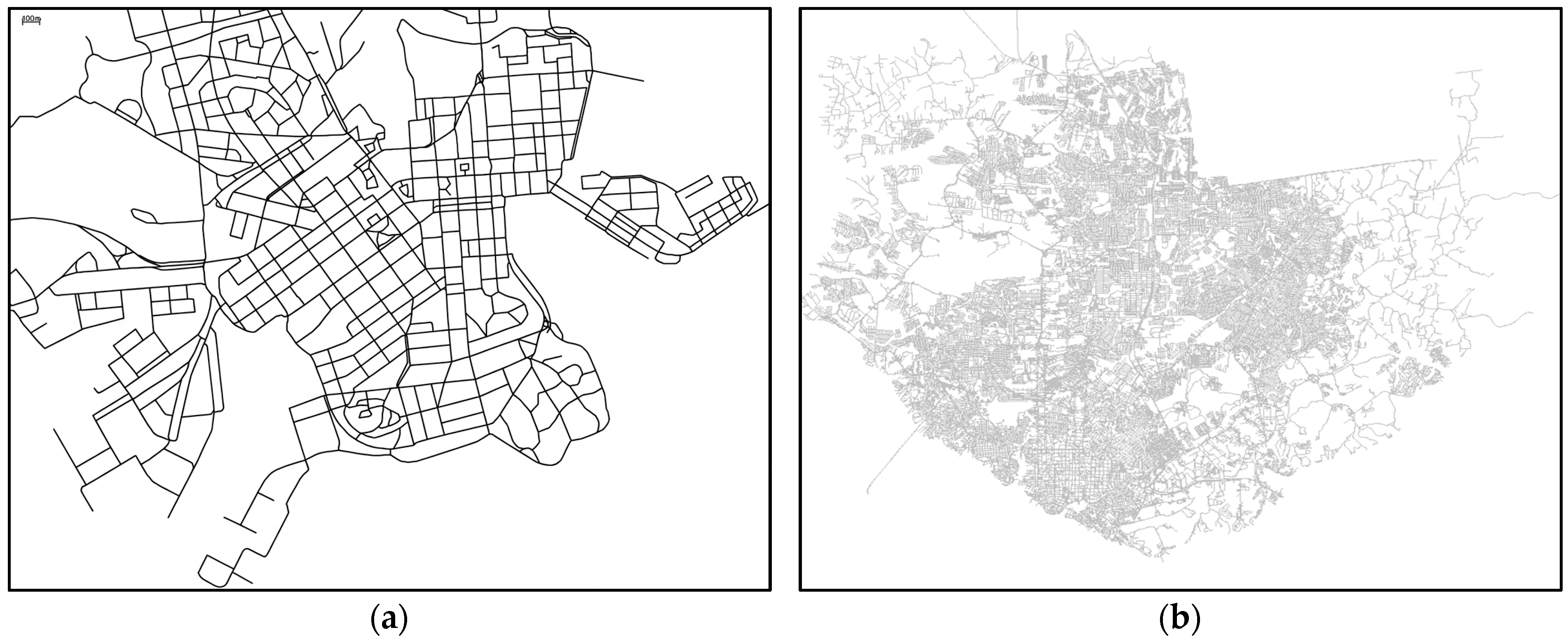
The evaluation encompassed two distinct mobility scenarios (Figure 3), utilizing spatial data initially extracted via Geographic Information Systems (GIS). To accurately reflect real-world topographical constraints within the Opportunistic Network Environment (ONE) simulator, these maps were converted into navigable routing topologies used by the Shortest Path Map-Based Movement (SPMBM) model. This internal representation abstracts traditional cartographic properties, retaining strictly the mathematical relative coordinates (X, Y) required for node mobility and pathfinding algorithms. The scenarios evaluated are:
  • Dense Pedestrian Network (Downtown Helsinki): A 4.5 × 3.4 km central urban area hosting 500 wearable IoT nodes. Devices operated at pedestrian speeds (0.5 to 1.5 m/s) utilizing Bluetooth Low Energy (BLE) interfaces, configured with a 10 m communication range and a 250 kBps transmission rate. This scenario evaluates protocol resilience against network congestion, frequent but brief encounters, and rapid buffer exhaustion. The energy model was parameterized based on typical IoT hardware (e.g., the Nordic nRF52 family).
  • Sparse Vehicular Network (Manaus): A large 35 × 35 km metropolitan road network extracted via OpenStreetMap (OSM) and QGIS. Representing a Vehicular Ad Hoc Network (VANET), 500 nodes traveled at vehicular speeds of 30 to 60 km/h. Communication relied on Wi-Fi 6 (IEEE 802.11ax) interfaces providing a 100 m range and a 25 MBps transmission rate. The energy model reflected onboard vehicular Wi-Fi modules (e.g., Panasonic PAN9019). This environment tests routing efficacy under fleeting, high-speed contact windows and geographic sparsity.
Although the mobility paths are generated by the SPMBM model, mapping them over real Geographic Information Systems (GIS) naturally induces realistic spatial bottlenecks and social hotspots (e.g., major intersections and urban centers). This topological constraint forces nodes into recurrent encounter patterns, providing a rigorous testbed for the Strength, Trend, and Regularity social metrics.
Table 1 summarizes the fixed general parameters established for both simulation environments.
The buffer limits evaluated in our scenarios (e.g., 10 MB to 80 MB for the Manaus network) were defined considering the multi-tasking nature of modern edge devices. Although Wi-Fi 6 modules interface with hardware capable of gigabyte-scale storage, opportunistic routing typically operates as a background service. In vehicular and wearable environments, this service is assigned a restricted application-level resource quota to prevent memory exhaustion for mission-critical processes (e.g., real-time vehicle control units). Imposing these constraints ensures a stringent evaluation, proving that QL-CASTRO maintains high reliability even when its operational slice of memory is intentionally limited.
Regarding the Reinforcement Learning configuration, the Q-learning rate α was calibrated to 0.3 . This value effectively balances stability and plasticity in non-stationary topologies. Learning coefficients above 0.5 prioritize recent encounters over historical delay estimates, which, in sparse topologies, allows sporadic encounters to heavily bias the stored values. The choice of α = 0.3 is mathematically consistent with recent opportunistic routing optimizations [60] and statistical convergence models [61], providing an optimal trade-off between historical knowledge retention and rapid environmental adaptation.
To ensure computational feasibility on highly constrained wearable and IoT devices, CASTRO and QL-CASTRO were rigorously evaluated for memory and energy overhead. To maintain numerical stability in long-term variance calculations, the protocol utilizes a condensed set of double-precision (8 bytes) statistical accumulators. As established in Section 2.3, the tabular Q-learning spatial complexity scales linearly O ( N ) . In the worst-case of the default density ( N = 500 nodes), the total memory footprint for the routing matrices, Q-tables, and Epidemic ACK delivery tables remains strictly below 150 KB. While this requirement targets high-tier IoT SoCs (e.g., nRF52840 with 256 KB RAM) and vehicular on-board units (OBU), it represents a strategic engineering trade-off to minimize radio frequency (RF) activity.
From an energy perspective, the cost of CPU-bound O ( 1 ) Q-table updates is negligible. To ensure empirical fidelity, the node energy model was parameterized using the Panasonic PAN9019 Wi-Fi 6 module specification [62]. The instant power consumption was calculated by aggregating the current draw from the 1.8 V and 3.3 V supply lines, yielding P t x = 0.640 W and P r x = 0.231 W. Conversely, based on the ARM Cortex-M4 datasheet [63], the processor consumes 12.26 μW/MHz. At a 64 MHz clock rate, the CPU consumes only 0.784 mW. Therefore, the protocol’s high-precision social intelligence is highly sustainable: it utilizes available static RAM to prevent redundant, high-power radio transmissions that would otherwise drain the battery.
Furthermore, the performance evaluation strictly adhered to a variable isolation methodology. As detailed in Table 2, a set of default values was established for the independent analysis variables. During each set of experiments, while a specific variable was iteratively scaled to observe its impact, all other parameters were maintained at their default values. This approach guarantees that any recorded performance fluctuations are caused exclusively by the parameter under observation.
Finally, the routing performance was systematically analyzed through four definitive metrics: (1) Delivery Ratio (%), indicating the percentage of successfully delivered messages out of the total generated; (2) Average Latency (min), measuring the mean time required for end-to-end payload transit; (3) Network Overhead, representing the ratio of redundant relayed copies to successful deliveries; and (4) Energy Consumption (J), quantifying the total energy depleted by the radio interfaces during transmission and reception operations.
To ensure the statistical reliability of the evaluations and mitigate the impact of stochastic variations inherent to opportunistic routing, every data point presented in the subsequent performance graphs represents the arithmetic mean of 15 independent simulation runs. The random seed associated with message generation was uniquely configured for each iteration via the simulator’s built-in settings.

3. Results

This section presents the performance evaluation of the proposed CASTRO and QL-CASTRO protocols compared to four consolidated baselines: PRoPHET, Spray and Wait (SnW), HESnW, and QoN-ASW. The analysis is divided according to the distinct mobility environments and investigates the impact of varying network parameters.

3.1. Performance in Dense Pedestrian Networks

3.1.1. Effect of Number of Nodes

The dense pedestrian scenario (Downtown Helsinki) is characterized by frequent encounters and a natural propensity for rapid buffer exhaustion. This configuration serves as a stress test to evaluate routing efficiency, congestion control, and resource management.
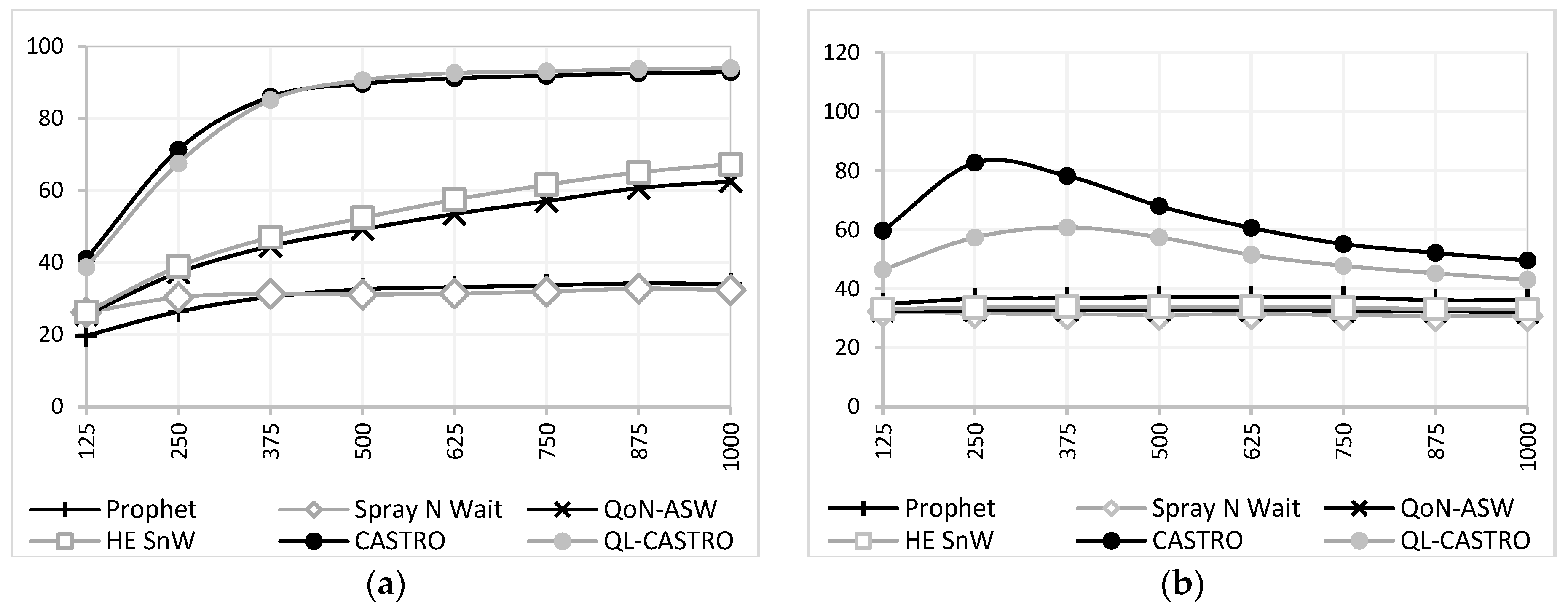
Varying the network density from 125 to 1000 nodes directly impacts the availability of routing opportunities and the volume of concurrent data exchanges. As illustrated in Figure 4a, both CASTRO and QL-CASTRO exhibit remarkable delivery rates. From 375 nodes onward, the proposed protocols surpass the 80% delivery mark, converging to over 90% in the densest configurations. In contrast, HESnW and QoN-ASW achieve between 60% and 70%, while PRoPHET and SnW remain near the 30% threshold. This significant performance gap demonstrates that the extraction of Strength, Trend, and Regularity metrics accurately maps the underlying social topology, ensuring that messages reliably reach their destinations even as structural complexity increases.
The average latency analysis (Figure 4b) highlights one of the advantages of the QL-CASTRO extension. The baseline CASTRO protocol exhibits an elevation in latency, reaching approximately 80 min at 250 nodes. This behavior is mathematically expected; because the protocol successfully delivers a massive volume of messages to hard-to-reach destinations, the global average transit time naturally rises. However, by introducing the Q-Learning dynamic delay estimate ( Q e s t ), QL-CASTRO actively mitigates prolonged message retention. The reinforcement learning layer flattens the latency curve to under 60 min across all densities, maintaining a strict temporal advantage over its predecessor. The lower average latencies (30 to 40 min) observed in baseline protocols correlate with their lower delivery rates, as successfully routed messages are predominantly those traversing shorter paths, reflecting a bias where messages with faster routes reach their destinations.
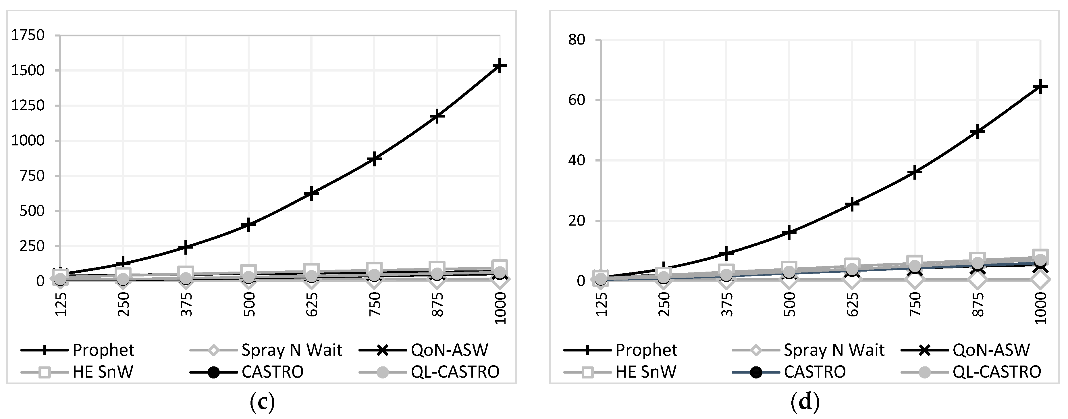
Regarding network overhead and energy consumption (Figure 4c,d), the pure flooding profile of PRoPHET generates exponential growth, exceeding 1500 in overhead and 60 J in energy depletion. When isolating the context-aware protocols, CASTRO and QL-CASTRO operate within highly sustainable margins, registering overheads between 40 and 60 and consuming approximately 6 J. These metrics are comparable to state-of-the-art models like QoN-ASW and HESnW, confirming that the asymmetric spray and active wait policies effectively prevent network saturation while maximizing data delivery.

3.1.2. Effect of Buffer Size

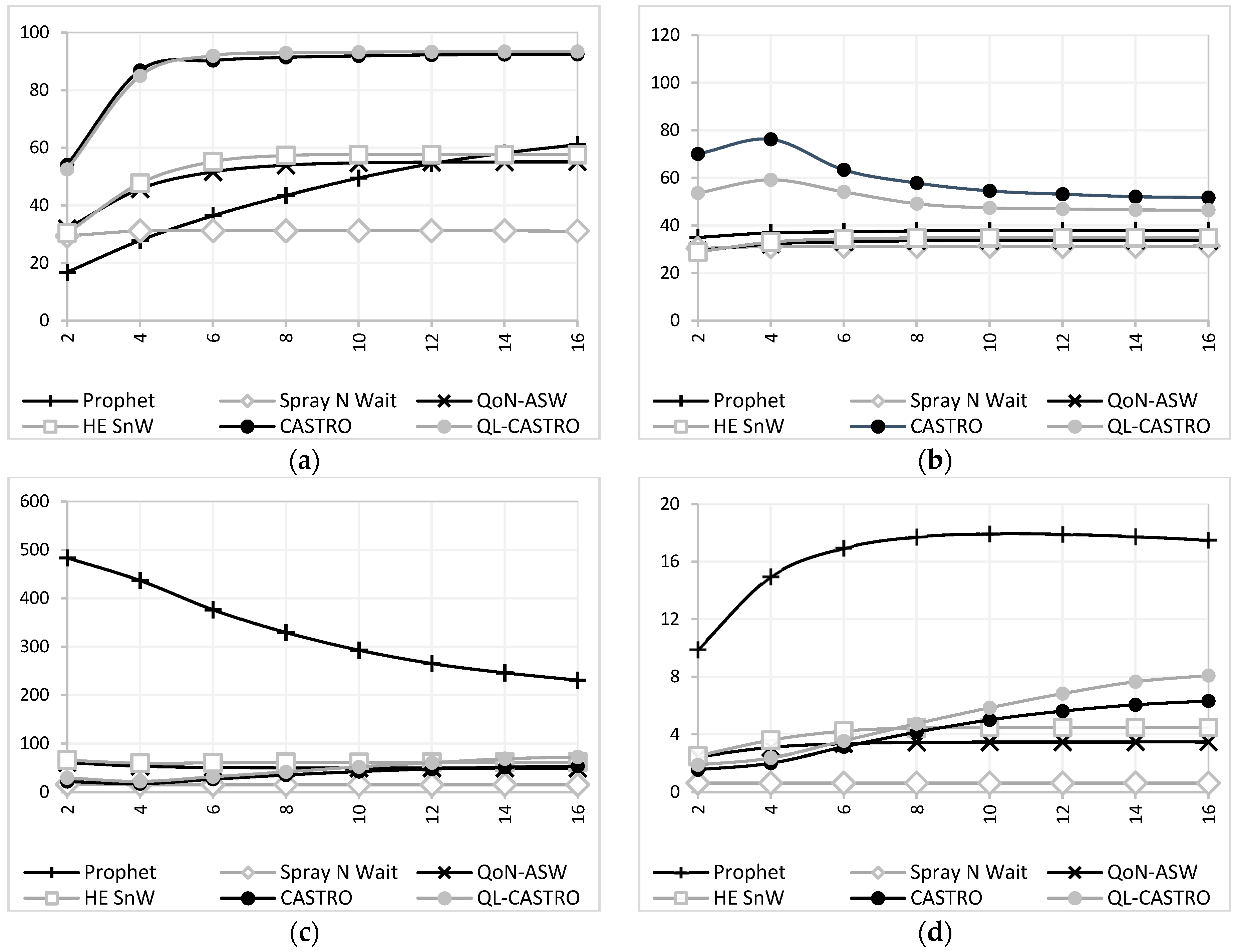
Restricting buffer capacity directly influences the likelihood of message drops due to memory overflow. As the buffer size varies between 2 MB and 16 MB, the delivery rate curves (Figure 5a) expose the resilience of the proposed models. Even under severe constraints (e.g., a 4 MB buffer), CASTRO and QL-CASTRO achieve approximately 85% delivery success. In contrast, competing protocols require significantly larger storage capacities to approach the 60% mark. This confirms the effectiveness of the preemptive acknowledgment and the TTL renewal mechanisms, which continuously remove successfully delivered data to accommodate new traffic and give more time for messages with high potential of delivery to traverse on the network.
In terms of latency (Figure 5b), severe memory constraints force the proposed protocols to limit forwarding attempts, holding messages for longer until optimal social contacts emerge. Once again, QL-CASTRO demonstrates superior control compared to its predecessor, maintaining the average delay below 60 min and gradually reducing this value as storage capacity expands, validating the Q-Learning delay estimation.
The network overhead and energy consumption metrics reveal a distinctive behavioral trait (Figure 5c,d). For CASTRO and QL-CASTRO, as the buffer expands from 2 MB to 16 MB, both overhead and energy consumption exhibit a slight, controlled increase. This phenomenon occurs because larger memory availability allows nodes to retain valid messages longer, enabling legitimate multi-hop transfers that would have otherwise been prematurely discarded. In contrast, protocols like PRoPHET, QoN-ASW and HESnW display a decreasing overhead alongside rising energy consumption. This shift is tied to their gradual improvement in delivery rates; as buffers grow, they deliver more messages, increasing the denominator in the overhead equation, but at the cost of more physical transmission and reception operations.

3.1.3. Effect of Message TTL

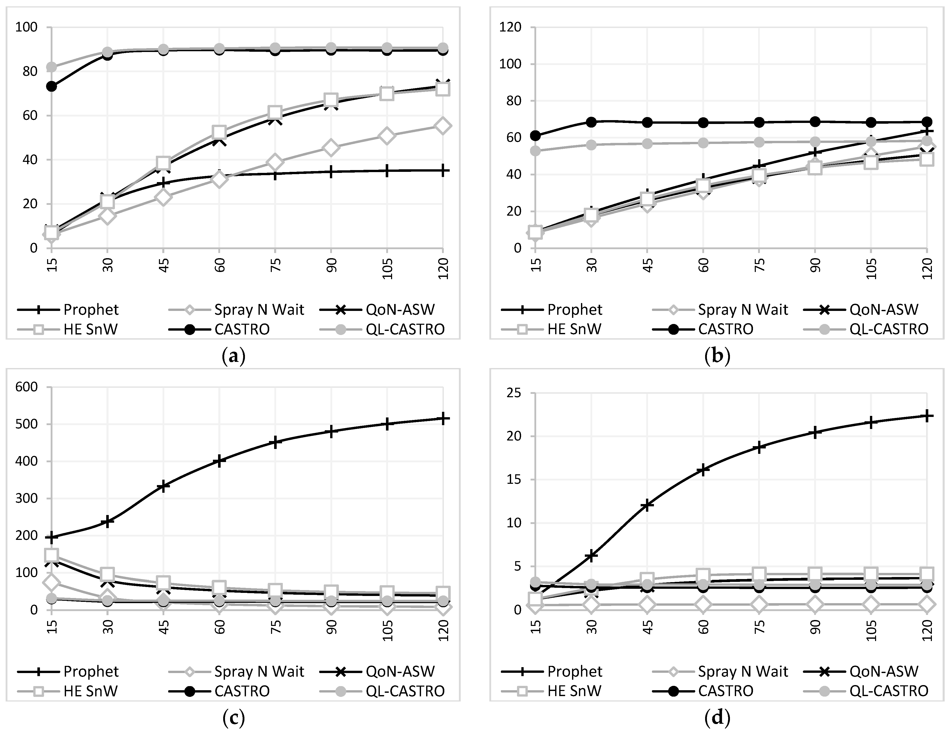
The Time-to-Live (TTL) parameter, evaluated between 15 and 120 min, dictates the maximum temporal window a message possesses to complete its routing trajectory. As illustrated by Figure 6a, restrictive TTL values severely penalize traditional algorithms, as messages frequently expire before reaching their destinations. This limitation is circumvented by the dynamic TTL renewal policy embedded in CASTRO and QL-CASTRO. By granting lifespan extensions to messages traversing highly consistent or faster paths, both proposed models converge to near 90% delivery success for TTL equal to 30 min, whereas the most efficient baseline protocols (QoN-ASW and HESnW) require 105 min of TTL to successfully deliver 70% of the generated payload.
In the average latency analysis (Figure 6b), baseline protocols exhibit reduced delays at lower TTLs, a behavior intrinsically tied to their lower delivery rates—only messages with immediate, short-path routes avoid expiration. As the TTL expands, allowing more complex trajectories to conclude successfully, the global latency naturally increases across all models. Notably, while the baseline CASTRO protocol reaches a latency peak near 70 min, QL-CASTRO uses its reinforcement learning to keep the average latency below 60 min, exhibiting a significantly flatter and more controlled curve even under permissive 120 min configurations.
The network overhead and energy consumption metrics further highlight the distinct resource management strategies (Figure 6c,d). The extended lifespan naturally provides more opportunities for encounters. For flooding-based models like PRoPHET, this extended window translates directly into redundant transmissions, resulting in an exponential surge in overhead and energy depletion. Conversely, CASTRO and QL-CASTRO maintain remarkably stable and bounded curves across the entire TTL spectrum. This stability confirms that the proposed forwarding policies restrict replication to socially or temporally advantageous paths, ensuring that an extended message lifespan does not inadvertently trigger communication channel saturation.

3.1.4. Effect of Generation Interval

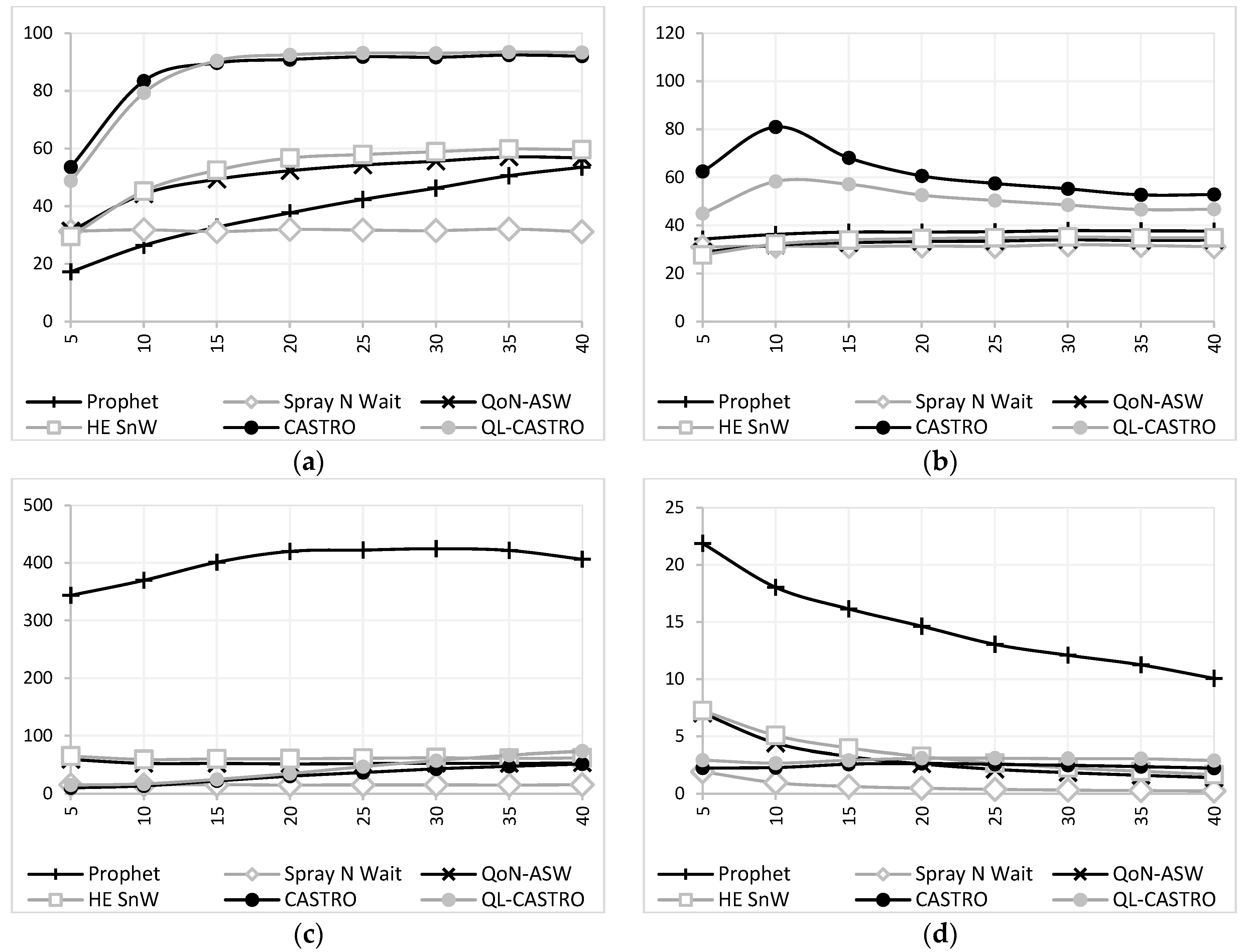
Varying the message generation interval from 5 to 40 s evaluates the network’s resilience against severe data congestion. Under maximum stress (5 s intervals), the continuous influx of newly generated messages rapidly exhausts available storage, forcing memory-constrained devices into premature message discards. Consequently, baseline protocols experience performance degradation, with delivery rates dropping to between 18% and 32%. In contrast, CASTRO and QL-CASTRO demonstrate significantly higher resilience, maintaining delivery rates above 50% even in this worst-case scenario (Figure 7a). As the generation interval expands to 15 s and beyond—alleviating buffer pressure—the proposed protocols rapidly converge to a 90% delivery success rate, whereas state-of-the-art models like HESnW and QoN-ASW achieve a success rate of approximately 60%.
The latency analysis further illustrates the behavioral dynamics of the protocols under heavy traffic (Figure 7b). The baseline CASTRO protocol exhibits a sharp escalation in average delivery time, peaking at approximately 80 min when the generation interval is 10 s. This peak reflects the continuous injection of messages coupled with the protocol’s conservative social retention policies. To effectively counteract this adverse effect, QL-CASTRO leverages the synergy between its dynamic delay estimations (Q-Learning), Newest-First queue management, and message retirement threshold. This strategic combination successfully suppresses the latency peak to roughly 60 min. As the generation interval continues to widen and network congestion eases, the average latency for QL-CASTRO gradually declines toward 45 min, continuously outperforming its predecessor.
The network overhead and energy consumption metrics reveal how the proposed algorithms dynamically adapt to available resources (Figure 7c,d). High data-generation frequencies severely penalize unconstrained protocols like PRoPHET, driving initial energy expenditure above 20 J due to redundant transmissions. In contrast, CASTRO and QL-CASTRO exhibit a unique, controlled behavior: as the generation interval widens (from 5 to 40 s), their overhead slightly increases from roughly 10 to 70. This phenomenon occurs because longer intervals yield more available buffer space, allowing the proposed algorithms to safely retain and forward legitimate multi-hop messages that would have otherwise been preemptively rejected under heavy traffic. Despite this targeted increase in relayed copies, their absolute energy consumption remains remarkably stable, consistently operating within the energy efficiency margins required by Bluetooth Low-Energy interfaces.

3.2. Performance in Sparse Vehicular Networks

3.2.1. Effect of Number of Nodes

The Manaus scenario represents a metropolitan-scale VANET. Characterized by high-speed mobility, fleeting contact windows, and geographic sparsity, this environment tests the routing protocols’ ability to discover and maintain viable multi-hop paths over vast distances without relying on continuous infrastructure.
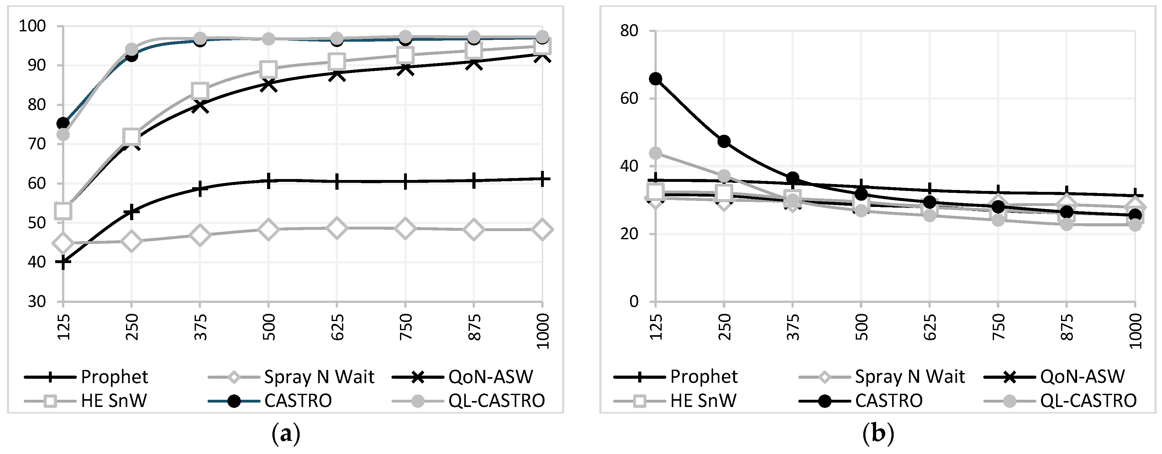
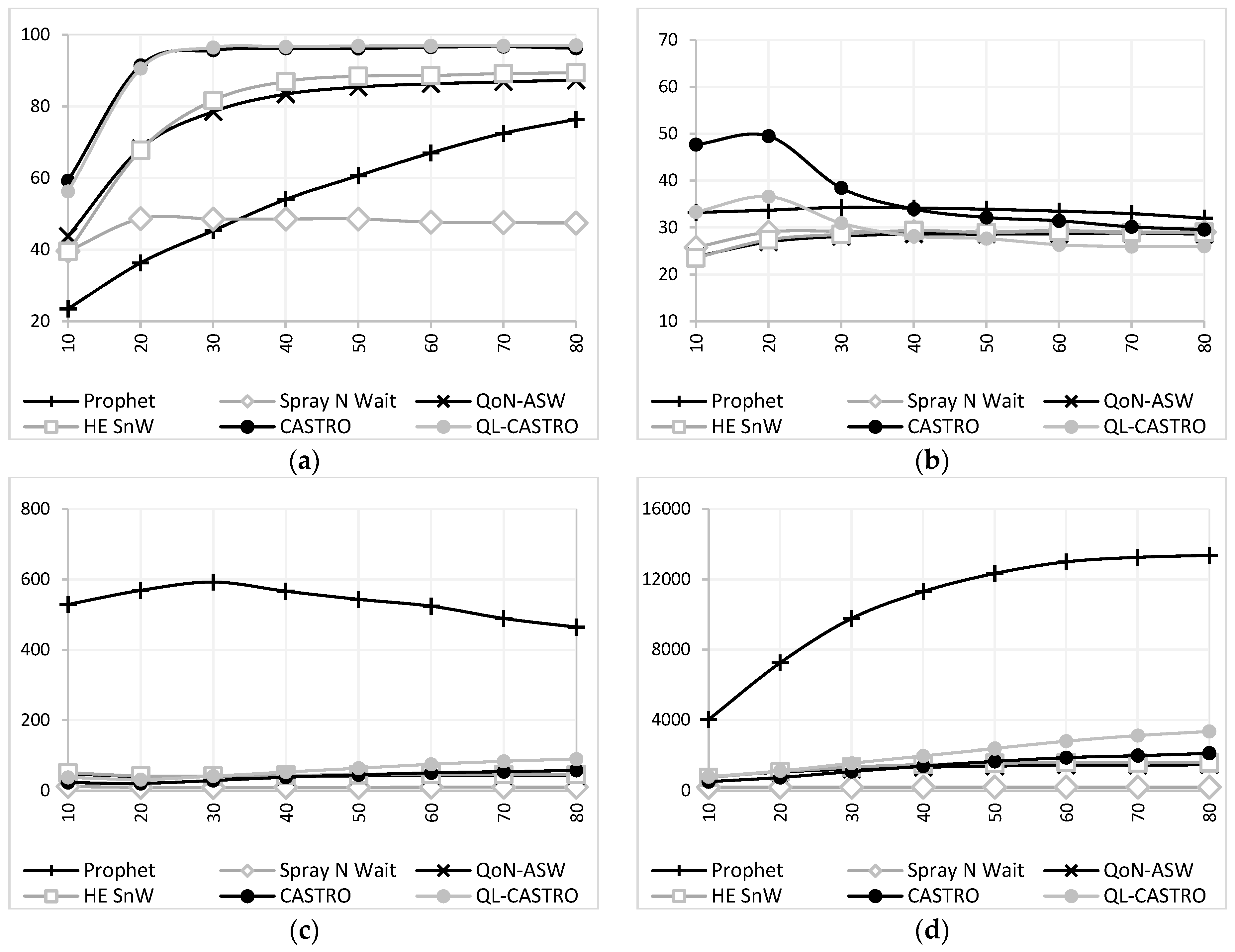
Evaluating the network density from 125 to 1000 vehicles reveals the resilience of the proposed models against geographic dispersion. As illustrated in Figure 8a, even in the sparsest configuration (125 nodes), CASTRO and QL-CASTRO achieve delivery rates approaching 75%. In contrast, recent baseline protocols such as HESnW and QoN-ASW register between 50% and 55%, while PRoPHET operates below 45%. As the network scales to 250 nodes and beyond, the proposed models rapidly converge to a 95% delivery success rate. This demonstrates high efficiency in exploiting the limited and brief encounter opportunities, proving that the social metrics effectively map the vehicular topology.
The average latency analysis (Figure 8.b) provides the clearest evidence of the Q-Learning architectural advantage in sparse environments. For the 125-node configuration, the baseline CASTRO protocol exhibits prolonged message retention while waiting for highly consistent social contacts, resulting in an average latency of 65 min. The introduction of QL-CASTRO immediately reduces this metric to approximately 45 min. More importantly, as node density increases, QL-CASTRO achieves the lowest latencies of the entire experiment, dropping to approximately 22 min at 1000 nodes. This continuous reduction substantiates that the reinforcement learning agent, strictly focused on minimizing the dynamic delay estimate ( Q e s t ), successfully optimizes the relay selection process for significantly faster data propagation.
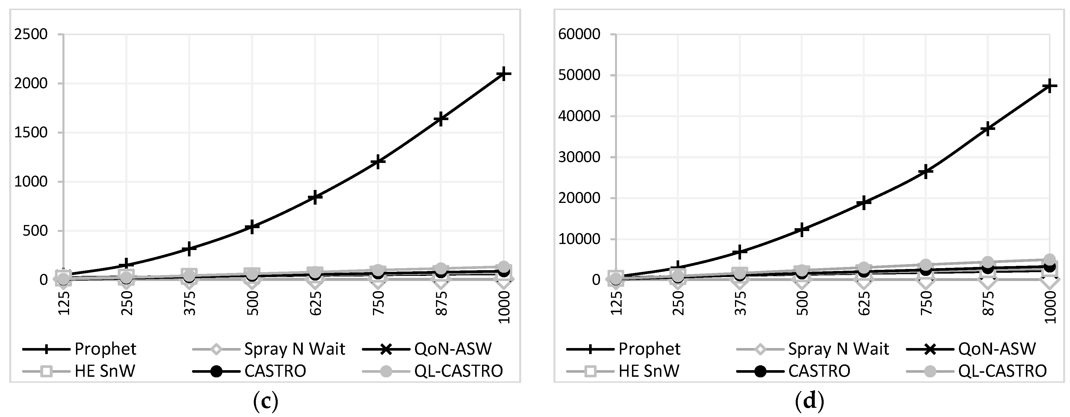
Regarding network overhead and energy consumption (Figure 8c,d), the unconstrained flooding nature of PRoPHET results in an exponential surge, surpassing an overhead of 2000 and severely draining network energy resources, rendering it impractical for real-world vehicular deployments. In stark contrast, CASTRO and QL-CASTRO maintain their overhead strictly below 140 across all densities. It is noteworthy that QL-CASTRO presents slightly higher overhead and energy consumption metrics than the baseline CASTRO protocol. This increment is a direct and mathematically expected consequence of the Q-Learning exploratory mechanism, where the autonomous agent must occasionally test new routes to converge on the optimal path. Considering the substantial reduction in delivery latency and the sustained high delivery rates, this energy expenditure represents a highly favorable and sustainable operational trade-off.

3.2.2. Effect of Buffer Size

Restricting the buffer capacity—evaluated from 10 MB to 80 MB—for messages of up to 5 MB imposes a high probability of message drops due to memory overflow. As illustrated by Figure 9a, this constraint significantly impairs probabilistic and flooding-based protocols. At the 10 MB threshold, algorithms such as PRoPHET, QoN-ASW, and HESnW suffer from premature discards, yielding delivery rates between 20% and 45%. CASTRO and QL-CASTRO protocols demonstrate more resilience, securing approximately 60% delivery success under the same constraints. As the buffer capacity expands to 20 MB and beyond, the proposed protocols rapidly converge to over 90% efficacy, capitalizing on social metrics, dynamic TTL renewals, and delivery acknowledgments to proactively free space for new traffic.
The average latency analysis (Figure 9b) highlights a defining characteristic of the socially conservative forwarding policy. In the baseline CASTRO protocol, an expansion to 20 MB provides enough storage to retain difficult-to-route messages, resulting in a latency peak near 50 min as the node waits for highly consistent contacts. However, QL-CASTRO effectively neutralizes this retention trap. By integrating Q-Learning delay estimates ( Q e s t ) with a Newest-First queue and a strict retirement threshold, the RL-enhanced model flattens the latency curve, reaching a peak near 36 min. Remarkably, as storage constraints ease (from 50 MB to 80 MB), QL-CASTRO leverages the available memory to explore faster routes, achieving the lowest average latency of the entire experiment—which is approximately 26 min.
The network overhead and energy consumption metrics underscore the distinct resource utilization strategies. Unconstrained replication inherently causes PRoPHET to experience an unsustainable surge, exceeding 12,000 J and an overhead of 500 as the buffer grows. Among the context-aware protocols, CASTRO and QL-CASTRO exhibit a deliberate, controlled upward trend. As memory becomes more available, both algorithms safely retain legitimate multi-hop messages for longer durations, resulting in a modest increase in relayed copies (overhead below 90) and energy consumption (approaching 3000 J for QL-CASTRO at 80 MB). This slight energetic increment in QL-CASTRO, compared to the base model, is the mathematical cost of the reinforcement learning’s exploratory mechanism. Given that this controlled exploration secures a reduction in latency while maintaining high delivery rates, the algorithm proves its capability to optimally balance computational overhead and routing efficiency in sparse vehicular environments.

3.2.3. Effect of Message TTL

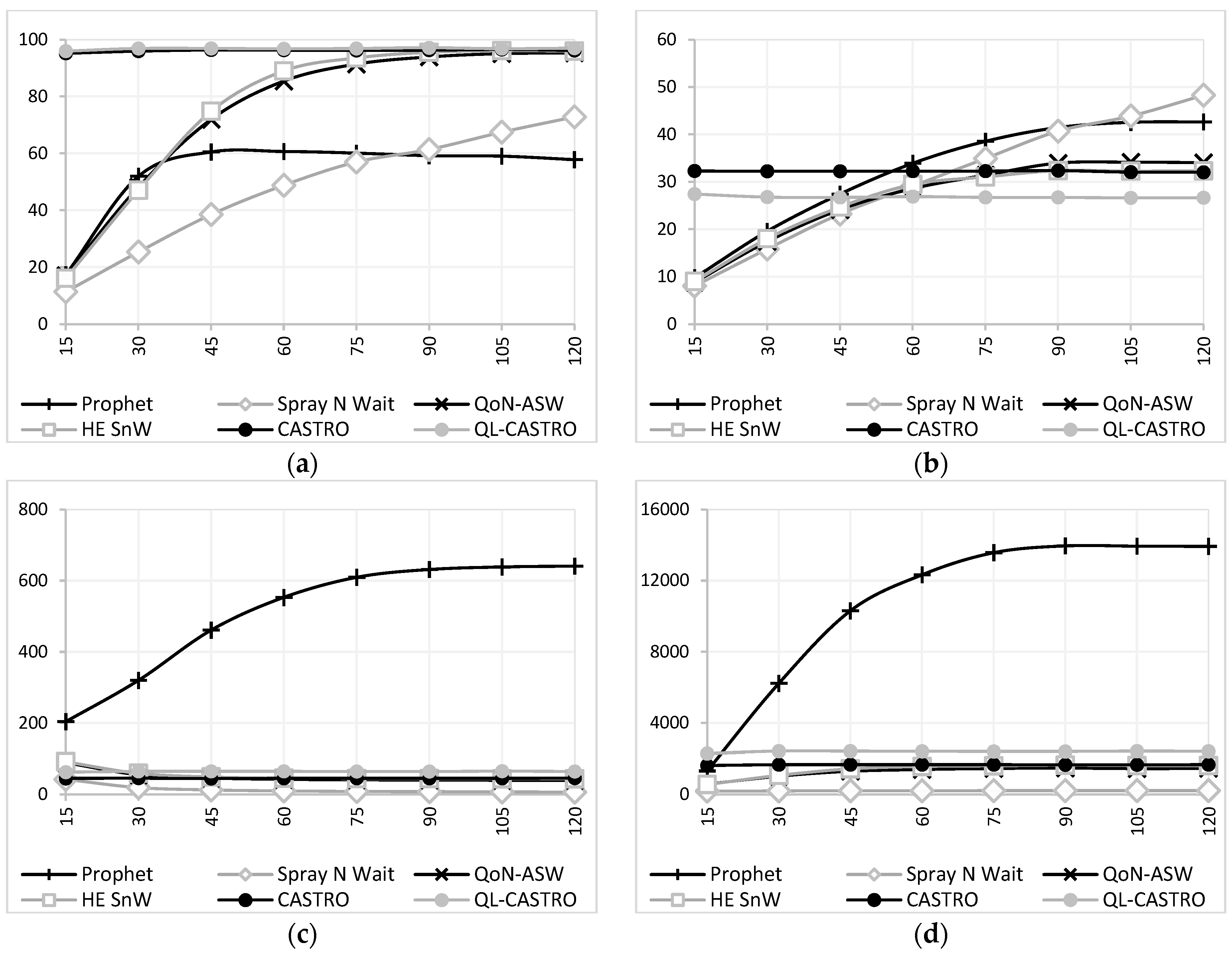
The Time-to-Live (TTL) parameter, evaluated between 15 and 120 min, defines the temporal window available for a message to traverse the sparse vehicular topology. In the most restrictive scenario (15 min), the vast geographic distances and fleeting contact opportunities penalize traditional routing algorithms. Baseline protocols struggle significantly, achieving delivery rates between 10% and 20% due to premature message expirations. In sharp contrast, CASTRO and QL-CASTRO leverage their dynamic TTL renewal policies. By granting mathematically calculated lifespan extensions to messages traversing highly consistent or faster trajectories, the proposed protocols sustain delivery rates above 90% even under the strict 15 min constraint, as illustrated by Figure 10a.
The average latency analysis (Figure 10b) provides a visualization of the protocols’ behavioral differences. For baseline algorithms, the latency starts low at a 15 min TTL. This is a consequence of their low delivery rates—only messages requiring immediate, single-hop transit survive, while others are dropped. As the TTL expands to 120 min, permitting more complex multi-hop trajectories, their average delays increase, with PRoPHET and SnW climbing past 40 min. Conversely, CASTRO and QL-CASTRO exhibit stable results. The baseline CASTRO protocol maintains a steady average of 32 min, while QL-CASTRO’s reinforcement learning optimization secures the lowest transit time at approximately 27 min. This proves that the message retirement policy ( A g e m a x ) and Newest-First queueing help protect the proposed models against the latency inflation typically caused by prolonged message lifespans.
The network overhead and energy consumption metrics (Figure 10c,d) expose the resource management flaws of flooding-based models under extended temporal windows. Unconstrained algorithms like PRoPHET exploit the additional time to blindly replicate data, resulting in a high overhead exceeding 600 and energy consumption climbing to 14,000 J (14 kJ). In contrast, CASTRO maintains a controlled diffusion, keeping energy consumption at roughly 1.5 kJ with an overhead of 45. QL-CASTRO registers a slightly higher total overhead (around 60) and energy metric (2.5 kJ). This increment is a direct consequence of the wider Q-Learning exploratory process. Nevertheless, this stable behavior ensures that extended lifespans can lead to very high delivery rates and reduce latency without saturating the vehicular communication channel.

3.2.4. Effect of Generation Interval

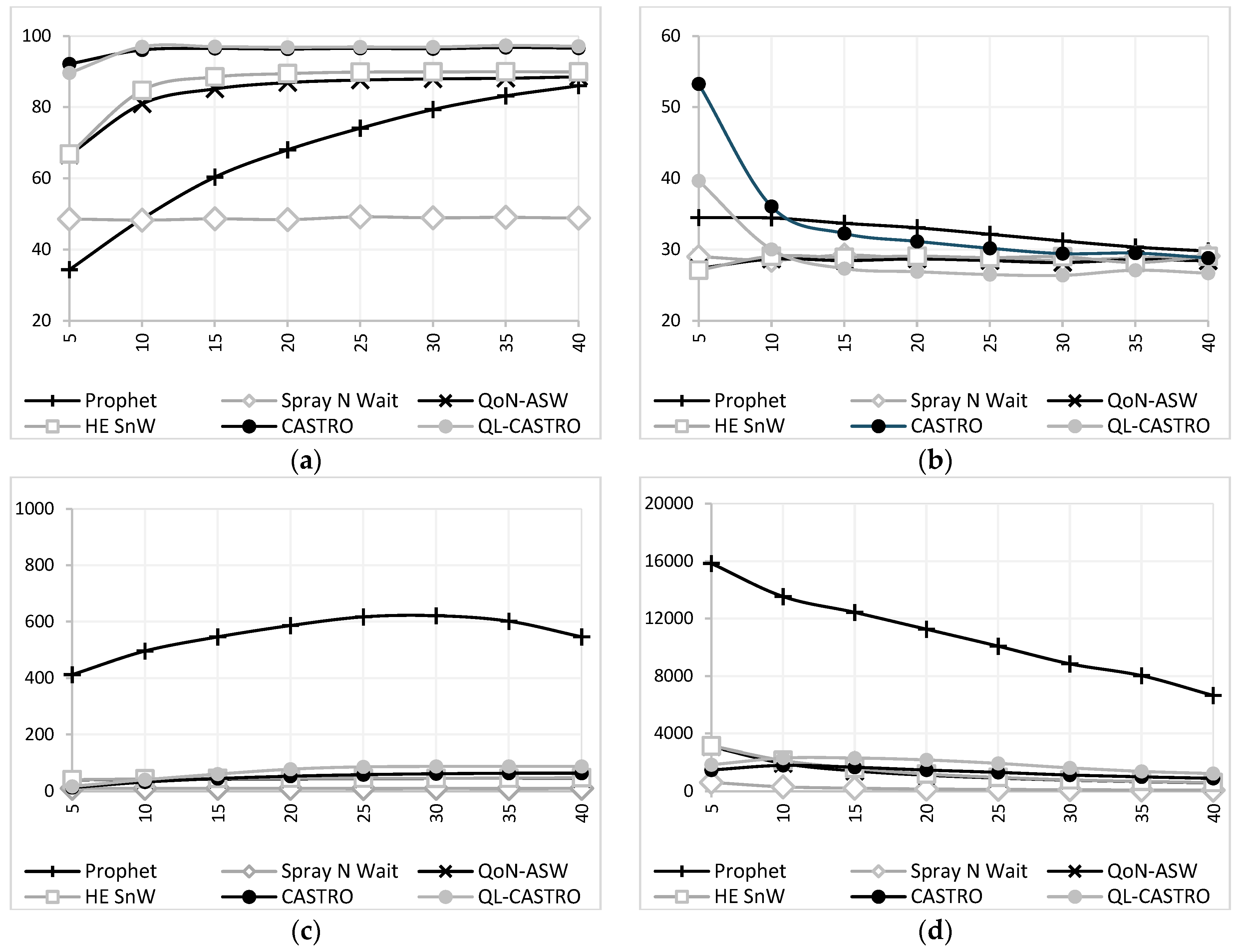
Varying the message generation interval from 5 to 40 s serves as a stress test, evaluating the VANET’s resilience against data congestion. At the maximum stress threshold (5 s intervals), the continuous influx of new payloads rapidly exhausts the local storage of mobile nodes, forcing premature message discards. Consequently, baseline protocols experience performance degradation (Figure 11a), with QoN-ASW and HESnW dropping to an approximately 65% delivery rate, and PRoPHET dropping to below 40%. In contrast, CASTRO and QL-CASTRO sustain delivery rates above 90% in the same scenario. This result confirms that restricting transmissions strictly to relays with proven social or temporal advantages protects the sparse network against congestion-induced losses.
The impact of conservative forwarding policies is prominently reflected in the average latency (Figure 11b). Under heavy traffic conditions (5 s intervals), the baseline CASTRO protocol experiences a sharp escalation in delivery time, peaking near 55 min. This behavior reflects the continuous injection of messages coupled with the protocol’s strict retention policy, where nodes wait for highly consistent social contacts while their buffers fill. To proactively counteract this adverse effect, QL-CASTRO leverages the synergy between its fast-route evaluations (Q-Learning), the prioritization of recent messages (Newest-First queue), and the dynamic message retirement threshold. This strategic combination successfully suppresses the maximum latency to under 40 min, ensuring timely data delivery even during peak network loads.
Finally, the network overhead and energy consumption metrics illustrate (Figure 11c,d) how the proposed protocols dynamically adapt to available resources. High data generation frequencies penalize traditional protocols, as the abundance of data drives them to maximize energy expenditure on redundant transmissions. Conversely, CASTRO and QL-CASTRO exhibit a slight, controlled increase in relayed copies as the generation interval widens (from 20 to 40 s). Longer intervals naturally yield more available buffer space, allowing the proposed algorithms to safely retain and forward legitimate multi-hop messages that would have otherwise been preemptively rejected under heavy traffic. This demonstrates that the QL-CASTRO protocol dynamically utilizes extra computational and memory resources to optimize routes, operating consistently within a highly sustainable energy margin without risking battery exhaustion.

4. Discussion

The experimental evaluations conducted across distinct mobility scenarios confirm the necessity of avoiding unconstrained replication mechanisms. Pure flooding, as seen in the Epidemic protocol, or unbounded probabilistic forwarding, as seen in PRoPHET, can cause severe resource depletion. Conversely, strictly limiting replication, like in Spray and Wait (SnW), averts congestion but severely restricts delivery rates in dynamic environments. Hybrid protocols (e.g., QoN-ASW and HESnW) partially bridge this gap. However, the proposed CASTRO protocol advances this paradigm by extracting specific social metrics: Strength, Trend, and Regularity. These metrics generate precise Routing Keys and global Consistencies. By employing these metrics during an Active Wait phase, CASTRO orchestrates intelligent forwarding decisions. This approach significantly elevates delivery rates compared to traditional methods. Furthermore, it effectively avoids the resource depletion inherent to unconstrained replication.
A defining characteristic of this controlled diffusion strategy is the protocol’s behavior upon copy exhaustion. When a node depletes its forwarding quota for a specific message ( L = 0 ), it does not discard the payload. Instead, it retains the message in the local buffer exclusively for a potential direct delivery. Consequently, the total number of message replicas organically expands beyond the initial spray limit. This allows for a broader spatial dispersion. Yet, because intermediate relaying halts once the quota is reached, this diffusion occurs at a highly regulated pace. This structural design effectively circumvents channel saturation, energy drain, and overflow losses.
Rigorous resource management policies further safeguard this controlled propagation. The buffer management system proactively removes previously delivered messages using exchanged acknowledgment tables. The results demonstrate that this mechanism significantly reduces network overhead. It also conserves battery life and minimizes message loss due to buffer overflow. Furthermore, the dynamic Time-to-Live (TTL) renewal mechanism emerges as a critical factor in maximizing delivery rates. The protocol grants lifespan extensions to messages traversing promising social trajectories. This prevents the premature dropping of viable data and ensures that routing efforts are not wasted by rigid expiration timers.
Despite the robustness of this socially conservative forwarding policy, the empirical data exposes an inherent trade-off: a natural elevation in average delivery latency. The integration of Reinforcement Learning in the QL-CASTRO extension successfully mitigates this drawback. The protocol fuses autonomous Q-Learning delay estimations with established social keys. This hybrid approach leverages a Newest-First queue and strict retirement thresholds. It effectively accelerates forwarding decisions without penalizing delivery rates or energy consumption.
We acknowledge that QL-CASTRO prioritizes delivery ratio and energy efficiency over ultra-low latency. However, its operational design is highly relevant to emerging frameworks, such as dynamic digital twin updates by adaptive model splitting [64]. In sparse environments, end-to-end connectivity is strictly opportunistic. Here, the delivery of outdated information functions as an uncertain data distortion. This stale data can induce severe errors in virtual–physical mapping. QL-CASTRO addresses this challenge by acting as a temporal filter. The social metrics, coupled with the strict message retirement policy, ensure that only data packets possessing an optimal Age of Information (AoI) consume constrained resources. This mechanism proactively filters obsolete sensory updates. Consequently, it preserves system fidelity in decentralized scenarios where infrastructure-dependent, low-latency communication is unfeasible.
Regarding network security, the decentralized store-carry-forward paradigm remains inherently susceptible to adversarial behaviors. Malicious relays could provide deceptive Q-learning estimates or fraudulent acknowledgments. To mitigate these vulnerabilities, the social indicators extracted by QL-CASTRO offer a potential analytical foundation for emerging Physical Layer Security (PLS) frameworks. Specifically, these metrics could support the formation of dynamic trilateral coalitions [65]. They serve as secondary indicators to verify node reliability and isolate eavesdroppers. Nevertheless, we identify a significant risk of Adversarial Mimicry. Cognitive adversaries may adopt deterministic mobility patterns to artificially inflate their social scores. This scenario exposes a potential limitation in game-theoretic models that assume a stochastic distinction between legitimate and malicious behaviors. Therefore, QL-CASTRO is positioned as a supportive layer for multi-factor defense strategies. Social reputation must be cross-referenced with physical-layer fingerprinting to ensure that trends and regularities are not leveraged as false trust indicators.
From a practical implementation standpoint, the mathematical formulation of both protocols deliberately avoids CPU bottlenecks. The resulting computational complexity ensures that these enhancements respect the processing restrictions of modern mobile hardware. The synergy between QL-CASTRO and high-tier edge hardware exemplifies a strategic transition toward Edge-driven Distributed Intelligence. By shifting the decisional complexity from the power-intensive radio interface to the processor’s static RAM, the architecture leverages localized memory to mitigate redundant retransmissions. This design is a fundamental prerequisite for next-generation Federated Learning and Digital Twin synchronization in Smart Cities. In these frameworks, decentralized nodes must evolve into autonomous intelligent agents. Preliminary efforts suggest that deploying QL-CASTRO as a background service on commercial smartphones is highly feasible. Future studies will focus on implementing dynamic physical interface handoffs. Devices could utilize BLE for continuous, energy-efficient neighbor discovery and seamlessly switch to high-bandwidth Wi-Fi 6 for large payload transmissions. Ultimately, this approach solidifies opportunistic routing as a viable, resource-efficient backbone for smart city infrastructures.

5. Conclusions

This study addressed the challenge of routing in resource-constrained Opportunistic Networks. We proposed the CASTRO architecture and its Reinforcement Learning extension, QL-CASTRO. Unlike traditional flooding or purely probabilistic models, the proposed protocols successfully model both connection and disconnection intervals. They evaluate Strength, Trend, and Regularity to restrict data replication exclusively to socially and temporally viable paths. The integration of Q-Learning in QL-CASTRO effectively mitigated the inherent latency limitations of conservative forwarding. The RL agent employed dynamic delay estimates, a Newest-First queue management, and strict message retirement policies. This allowed it to accelerate forwarding decisions without saturating the communication channel. Extensive simulations across dense pedestrian (Helsinki) and sparse vehicular (Manaus) environments validated our approach. Both models sustained delivery rates near 90%. They significantly outperformed baseline protocols (PRoPHET, SnW, HESnW, and QoN-ASW) under severe buffer and TTL constraints. Furthermore, QL-CASTRO successfully kept network overhead and energy consumption within the strict margins required by IoT devices. Future work will focus on transitioning these theoretical frameworks into real-world physical deployments. We will explore dynamic interface handoffs (e.g., BLE to Wi-Fi 6) to further solidify opportunistic routing as a scalable backbone for smart city infrastructures.

Author Contributions

W.C.d.R.: Conceptualization, Data curation, Formal analysis, Investigation, Methodology, Software, Validation, Writing—original draft, Writing—review and editing. C.B.C.: Conceptualization, Funding acquisition, Methodology, Project administration, Resources, Supervision, Writing—review and editing. M.W.R.d.S.: Conceptualization, Methodology, Writing—review and editing. R.M.G.: Conceptualization, Methodology, Writing—review and editing. A.C.M.: Conceptualization, Methodology, Writing—review and editing. W.S.S.J.: Funding acquisition, Resources, Supervision. All authors have read and agreed to the published version of the manuscript.

Funding

This research was funded by the Government of the State of Amazonas through the State Funding Agency of Amazonas (FAPEAM), under the Postgraduate Stricto Sensu Support Program (POSGRAD), Edition 2021–2022, through a scholarship award established by FAPEAM Resolution No. 006/2021, under Call/Resolution No. 008/2021 (POSGRAD 2021/2022–UFAM).

Data Availability Statement

The original contributions presented in this study are included in the article. Further inquiries can be directed to the corresponding author(s).

Conflicts of Interest

The authors declare no conflicts of interest. The funders had no role in the design of the study; in the collection, analyses, or interpretation of data; in the writing of the manuscript; or in the decision to publish the results.

Appendix A. Proof of Maximum Variance for Connection Regularity

To normalize the Connection Regularity metric (Equation (7)), it is necessary to determine the maximum possible variance for a set of discrete time intervals.
Theorem A1.
Given a set of  N  positive integers, whose sum of elements is represented by  C , the maximum sum of squares is obtained when one element of the set is equal to  C ( N 1 )  and the remaining  N 1  elements are equal to 1.
Proof. 
Let A = { a 1 , a 2 , , a N } be a set of N positive integers. The sum of the elements of A is denoted by C A , and the sum of their squares is denoted by Q A . The objective is to determine the values for the elements of A such that Q A reaches its maximum possible value. □
Assume a set of values A = { x , 1 , , 1 } , where x = C A ( N 1 ) . In this configuration, the sum of the squares is given by:
Q A = x 2 + N 1 .
Next, we evaluate an alternative combination of values for a set Y . Let y be a positive integer such that y = y 1 + y 2 + + y N 1 , where all addends are non-negative integers. We subtract y from x and distribute its addends among the remaining elements of A . The resulting set is Y , and the sum of the squares of its elements is given by Q Y :
Y = { x y ,   1 + y 1 ,   1 + y 2 , , 1 + y N 1 } ,
Q Y = x y 2 + 1 + y 1 2 + 1 + y 2 2 + + 1 + y N 1 2 .
Expanding the binomials, the sum of squares can be rewritten as:
Q Y = x y 2 + N 1 + 2 y + n = 1 N 1 y n 2 .
By applying the algebraic expansion of the square of the multinomial y = y 1 + y 2 + + y N 1 , we establish the following relationship:
n = 1 N 1 y n 2 = y 2 2 1 n < m N 1 ( y n   y m ) .
Substituting Equation (A4) into Equation (A3), we obtain:
Q Y = x 2 2 x y + y 2 + N 1 + 2 y + y 2 2 1 n < m N 1 ( y n   y m ) .
By inserting Equation (A1) into Equation (A5) and factoring the terms, we arrive at:
Q Y = Q A 2 y x y 1 + 1 n < m N 1 ( y n   y m ) .
Since the elements of set Y are strictly positive integers, it follows that x y 1 . Therefore, Q A Q Y holds true for all 0 y x 1 . The equality Q A = Q Y is observed if and only if y = 0 , which ensures that the subtrahends in Equation (A6) equal zero, meaning the sets A and Y are identical.
Thus, the maximum sum of squares for a set of N positive integers with a fixed sum is obtained when Q A = Q Y , corresponding to the exact case where one element is equal to C A ( N 1 ) and all other elements are equal to 1. This mathematical premise directly substantiates the maximum variance formula applied in Equation (6).

References

  1. Kolesnyk, K.; Kozemchuk, I. Analysis of methods and tools for designing embedded systems of the internet of things. CDS 2025, 7, 229–239. [Google Scholar] [CrossRef]
  2. Zreikat, A.I.; AlArnaout, Z.; Abadleh, A.; Elbasi, E.; Mostafa, N. The Integration of the Internet of Things (IoT) Applications into 5G Networks: A Review and Analysis. Computers 2025, 14, 250. [Google Scholar] [CrossRef]
  3. Oliveira, F.; Costa, D.G.; Assis, F.; Silva, I. Internet of Intelligent Things: A convergence of embedded systems, edge computing and machine learning. Internet Things 2024, 26, 101153. [Google Scholar] [CrossRef]
  4. Zhang, S.; He, N.; Li, Z.; Fu, Q.; Liang, W.; Xiong, N.N. A Survey on Mobile Crowd Sensing: Concepts, Applications, Technologies, and Future Directions. IEEE Internet Things J. 2025, 12, 52090–52109. [Google Scholar] [CrossRef]
  5. Mendez, J.; Bierzynski, K.; Cuéllar, M.P.; Morales, D.P. Edge Intelligence: Concepts, Architectures, Applications, and Future Directions. ACM Trans. Embed. Comput. Syst. 2022, 21, 48. [Google Scholar] [CrossRef]
  6. Chen, R.; Yi, C.; Zhou, F.; Kang, J.; Wu, Y.; Niyato, D. Federated Digital Twin Construction via Distributed Sensing: A Game-Theoretic Online Optimization With Overlapping Coalitions. IEEE Trans. Mob. Comput. 2025, 24, 12221–12238. [Google Scholar] [CrossRef]
  7. Zheng, K.; Luo, R.; Liu, X.; Qiu, J.; Liu, J. Distributed DDPG-Based Resource Allocation for Age of Information Minimization in Mobile Wireless-Powered Internet of Things. IEEE Internet Things J. 2024, 11, 29102–29115. [Google Scholar] [CrossRef]
  8. Gautam, T.; Dev, A. Opportunistic network routing protocols: Challenges, implementation and evaluation. In Proceedings of the 2019 9th International Conference on Cloud Computing, Data Science & Engineering (Confluence); IEEE: Piscataway, NJ, USA, 2019; pp. 100–106. [Google Scholar]
  9. Baudic, G.; Auger, A.; Ramiro, V.; Lochin, E. Using emulation to validate applications on opportunistic networks. In Advances in Delay-Tolerant Networks (DTNs) Architecture and Enhanced Performance, 2nd ed.; Elsevier: Amsterdam, The Netherlands, 2020; pp. 273–280. [Google Scholar]
  10. Bacanli, S.S.; Turgut, D. Energy-efficient unmanned aerial vehicle scanning approach with node clustering in opportunistic networks. Comput. Commun. 2020, 161, 76–85. [Google Scholar] [CrossRef]
  11. López-Villegas, I.; Martínez-Rios, E.A.; Izquierdo-Reyes, J.; Bustamante-Bello, R.; Falcone, F. A systematic literature review of emergency communications assisted by unnamed aerial vehicles. Ad Hoc Netw. 2026, 182, 104063. [Google Scholar] [CrossRef]
  12. Vegni, A.M.; Iglesias, C.B.; Loscrí, V. MOVES: A memOry-based VEhicular social forwarding technique. Comput. Netw. 2021, 197, 108304. [Google Scholar] [CrossRef]
  13. Saleem, Y.; Mitton, N.; Loscri, V. DIVINE: Data offloading in vehicular networks with QoS provisioning. Ad Hoc Netw. 2021, 123, 102636. [Google Scholar] [CrossRef]
  14. Abbas, A.; Krichen, M.; Alroobaea, R.; Malebary, S.; Tariq, U.; Piran, M.J. An opportunistic data dissemination for autonomous vehicles communication. Soft Comput. 2021, 25, 11899–11912. [Google Scholar] [CrossRef]
  15. Ayele, E.D.; Meratnia, N.; Havinga, P.J.M. Towards a new opportunistic IoT network architecture for wildlife monitoring system. In Proceedings of the 2018 9th IFIP International Conference on New Technologies, Mobility and Security (NTMS); IEEE: Piscataway, NJ, USA, 2018; pp. 1–5. [Google Scholar]
  16. Wu, H.; Han, X.; Zhu, H.; Chen, C.; Yang, B. An efficient opportunistic routing protocol with low latency for farm wireless sensor networks. Electronics 2022, 11, 1936. [Google Scholar] [CrossRef]
  17. Xian, J.; Wu, H.; Mei, X.; Chen, X.; Yang, Y. Low-delay and energy-efficient opportunistic routing for maritime search and rescue wireless sensor networks. Remote Sens. 2022, 14, 5178. [Google Scholar] [CrossRef]
  18. Prasad, A.; Gurung, S.; Sharma, K. Challenges and opportunities to enhance buffer management for disaster area in delay tolerant network: A review with performance analysis. In Proceedings of the 2024 International Conference on Electrical Electronics and Computing Technologies (ICEECT), Greater Noida, India, 29–31 August 2024. [Google Scholar]
  19. Ezife, F.; Li, W.; Yang, S. A survey of buffer management strategies in delay tolerant networks. In Proceedings of the 2017 IEEE 14th International Conference on Mobile Ad Hoc and Sensor Systems (MASS); IEEE: Piscataway, NJ, USA, 2017; pp. 599–603. [Google Scholar]
  20. Majeed, M.R.; Naeem, F.; Salam, A.; Khan, W.U.; Irfanullah, S. Enhanced buffer management scheme to avoid congestion in delay tolerant social network. In Proceedings of the 2018 IEEE 21st International Multi-Topic Conference (INMIC), Karachi, Pakistan, 1–2 November 2018. [Google Scholar]
  21. Biabani, M.; Yazdani, N.; Fotouhi, H. EE-MSWSN: Energy-efficient mobile sink scheduling in wireless sensor networks. IEEE Internet Things J. 2022, 9, 18360–18377. [Google Scholar] [CrossRef]
  22. Sreya, K.; Rajyalaxmi, M.; Nireesha, K.; Kumar, K.P.; Bhavani, A. Review on energy consumption in delay tolerant network (DTN). In Proceedings of the International Conference on IoT Based Control Networks and Intelligent Systems (ICICNIS); IEEE: Piscataway, NJ, USA, 2024; pp. 656–663. [Google Scholar]
  23. Lent, R. Experimental evaluation of a cognitive routing strategy for efficient energy management in DTN. IEEE J. Radio Freq. Identif. 2024, 8, 506–515. [Google Scholar] [CrossRef]
  24. Çelebi, H.; Yapici, Y.; Güvenç, İ.; Schulzrinne, H. Load-based On/Off scheduling for energy-efficient delay-tolerant 5G networks. IEEE Trans. Green Commun. Netw. 2019, 3, 955–970. [Google Scholar] [CrossRef]
  25. Wang, E.; Yang, Y.; Wu, J. Energy efficient beaconing control strategy based on time-continuous Markov model in DTNs. IEEE Trans. Veh. Technol. 2017, 66, 7411–7421. [Google Scholar] [CrossRef]
  26. Bharamagoudar, S.R.; Saboji, S.V. Routing in opportunistic networks: Taxonomy, survey. In Proceedings of the 2017 International Conference on Electrical, Electronics, Communication, Computer, and Optimization Techniques (ICEECCOT); IEEE: Piscataway, NJ, USA, 2017; pp. 301–306. [Google Scholar]
  27. Avoussoukpo, C.B.; Ogunseyi, T.B.; Tchenagnon, M. Securing and facilitating communication within opportunistic networks: A holistic survey. IEEE Access 2021, 9, 55009–55038. [Google Scholar] [CrossRef]
  28. Vahdat, A.; Becker, D. Epidemic Routing for Partially Connected Ad Hoc Networks. In Technical Report CS-200006; Department of Computer Science, Duke University: Durham, NC, USA, 2000. [Google Scholar]
  29. Spyropoulos, T.; Psounis, K.; Raghavendra, C.S. Spray and wait: An efficient routing scheme for intermittently connected mobile networks. In Proceedings of the 2005 ACM SIGCOMM Workshop on Delay-Tolerant Networking (WDTN ‘05); ACM: New York, NY, USA, 2005; pp. 252–259. [Google Scholar]
  30. Spyropoulos, T.; Psounis, K.; Raghavendra, C.S. Efficient routing in intermittently connected mobile networks: The multiple-copy case. IEEE/ACM Trans. Netw. 2008, 16, 77–90. [Google Scholar] [CrossRef]
  31. Huang, F.; Cui, J.; Chang, Y.; Wang, T.; Wang, M.; Yang, Y. An improved spray and wait routing algorithm based on stable transmission capacity evaluation of nodes in opportunistic network. Int. J. Distrib. Sens. Netw. 2024, 20, 7471329. [Google Scholar] [CrossRef]
  32. Lindgren, A.; Doria, A.; Schelén, O. Probabilistic routing in intermittently connected networks. ACM SIGMOBILE Mob. Comput. Commun. Rev. 2003, 7, 19–20. [Google Scholar] [CrossRef]
  33. Peng, D.; Chang, Y.; Duan, X.; Cui, J. A predictiveness-enhanced PRoPHET based on triple exponential smoothing in mobile opportunistic networks. In Proceedings of the 2024 International Conference on Ubiquitous Communication (Ucom); IEEE: Piscataway, NJ, USA, 2024; pp. 314–319. [Google Scholar]
  34. Basu, S.; Biswas, A.; Roy, S.; Dasbit, S. Wise-PRoPHET: A watchdog supervised PRoPHET for reliable dissemination of post disaster situational information over smartphone based DTN. J. Netw. Comput. Appl. 2018, 109, 11–23. [Google Scholar] [CrossRef]
  35. Bista, B.B.; Rawat, D.B. Enhancement of PRoPHET routing in delay tolerant networks from an energy prospective. In Proceedings of the 2016 IEEE Region 10 Conference (TENCON); IEEE: Piscataway, NJ, USA, 2016; pp. 1579–1582. [Google Scholar]
  36. Chen, J.; Bie, P.; Nie, J.; Wei, Z. HP-ECD: Heuristic prophet protocol based on energy balance, cache optimization, and asynchronous dormancy. J. King Saud Univ. Comput. Inf. Sci. 2024, 36, 101861. [Google Scholar] [CrossRef]
  37. Han, S.D.; Chung, Y.W. An improved PRoPHET routing protocol in delay tolerant network. Sci. World J. 2015, 2015, 623090. [Google Scholar] [CrossRef] [PubMed]
  38. Lee, E.H.; Seo, D.Y.; Chung, Y.W. An efficient routing protocol using the history of delivery predictability in opportunistic networks. Appl. Sci. 2018, 8, 2215. [Google Scholar] [CrossRef]
  39. Zhang, J.; Huang, H.; Min, G.; Miao, W.; Wu, D. Social-aware routing in mobile opportunistic networks. IEEE Wirel. Commun. 2021, 28, 152–158. [Google Scholar] [CrossRef]
  40. Tulu, M.M.; Mkiramweni, M.E.; Hou, R.; Feisso, S.; Younas, T. Influential nodes selection to enhance data dissemination in mobile social networks: A survey. J. Netw. Comput. Appl. 2020, 169, 102768. [Google Scholar] [CrossRef]
  41. Li, B.; Gao, Z.; Shan, X.; Zhou, W.; Ferrara, E. SoReC: A social-relation based centrality measure in mobile social networks. arXiv 2019, arXiv:1902.09489. [Google Scholar]
  42. Chen, D.; Cui, H.; Welsch, R.E. An adaptive routing algorithm based on relation tree in DTN. Sensors 2021, 21, 7847. [Google Scholar] [CrossRef]
  43. Gan, S.; Zhou, J.; Wei, K. HESnW: History encounters-based spray-and-wait routing protocol for delay tolerant networks. J. Inf. Process. Syst. 2017, 13, 618–629. [Google Scholar]
  44. Cui, J.; Cao, S.; Chang, Y.; Wu, L.; Liu, D.; Yang, Y. An adaptive spray and wait routing algorithm based on quality of node in delay tolerant network. IEEE Access 2019, 7, 35274–35286. [Google Scholar] [CrossRef]
  45. Cui, J.; Wu, Y.; Chang, Y.; Sun, J.; Yu, D. Probabilistic routing algorithm based on connection separation time in delay tolerant network. J. Chin. Comput. Syst. 2023, 44, 1257–1265. [Google Scholar]
  46. Liaq, M.; Sharif, S.; Zeadally, S.; Ejaz, W. Utilization of machine learning in future wireless networks for resource optimization: A survey. Ad Hoc Netw. 2025, 178, 103983. [Google Scholar] [CrossRef]
  47. Gandhi, J.; Narmawala, Z. A comprehensive survey on machine learning techniques in opportunistic networks: Advances, challenges and future directions. Pervasive Mob. Comput. 2024, 100, 101917. [Google Scholar] [CrossRef]
  48. Alaoui, E.A.A.; Tekouabou, S.C.K.; Maleh, Y.; Nayyar, A. Towards to intelligent routing for DTN protocols using machine learning techniques. Simul. Model. Pract. Theory 2022, 117, 102475. [Google Scholar] [CrossRef]
  49. Oualhaj, O.A.; Kobbane, A.; Ben-Othman, J. A decentralized control of autonomous delay tolerant networks: Multi agents Markov decision processes framework. In Proceedings of the 2018 IEEE International Conference on Communications (ICC); IEEE: Piscataway, NJ, USA, 2018; pp. 1–6. [Google Scholar]
  50. Saad, A.; Yan, P.; De Grande, R.E. MDP-based connectivity and availability models for internet of vehicles. Internet Things 2023, 24, 100963. [Google Scholar] [CrossRef]
  51. Elsayed, M.; Vasan, G.; Mahmood, A.R. Deep Reinforcement Learning Without Experience Replay, Target Networks, or Batch Updates. In Proceedings of the 38th Workshop on Fine-Tuning in Machine Learning (NeurIPS), Vancouver, BC, Canada, 14 December 2024. [Google Scholar]
  52. Lin, J.; Zhu, L.; Chen, W.M.; Wang, W.C.; Gan, C.; Han, S. On-device training under 256 kb memory. Adv. Neural Inf. Process. Syst. 2022, 35, 22941–22954. [Google Scholar]
  53. Abdulazeez, D.H.; Askar, S.K. Offloading mechanisms based on reinforcement learning and deep learning algorithms in the fog computing environment: A comprehensive review. IEEE Access 2023, 11, 12555–12586. [Google Scholar] [CrossRef]
  54. Lim, W.Y.B.; Luong, N.C.; Hoang, D.T.; Jiao, Y.; Liang, Y.C.; Yang, Q.; Niyato, D.; Miao, C. Federated Learning in Mobile Edge Networks: A Comprehensive Survey. IEEE Commun. Surv. Tutor. 2020, 22, 2031–2063. [Google Scholar] [CrossRef]
  55. Sammou, E.M. Intelligent routing agent based on Q-learning and Markov decision processes for routing optimization in DTN networks. Int. J. Intell. Netw. 2025, 6, 97–112. [Google Scholar] [CrossRef]
  56. Liu, L.; Wang, R.; Wu, J. A time-inhomogeneous Markov chain and its distributed solution for message dissemination in OUSNs. J. Parallel Distrib. Comput. 2019, 130, 179–192. [Google Scholar] [CrossRef]
  57. Watkins, C.J.C.H.; Dayan, P. Q-learning. Mach. Learn. 1992, 8, 279–292. [Google Scholar] [CrossRef]
  58. Sutton, R.S.; Barto, A.G. Reinforcement Learning: An Introduction, 2nd ed.; MIT Press: Cambridge, MA, USA, 2018. [Google Scholar]
  59. Mammeri, Z. Reinforcement learning based routing in networks: Review and classification of approaches. IEEE Access 2019, 7, 55916–55950. [Google Scholar] [CrossRef]
  60. Duenas Santos, C.L.; Mezher, A.M.; Astudillo León, J.P.; Cardenas Barrera, J.; Castillo Guerra, E.; Meng, J. Q-Learning-Based Routing Protocol for Advanced Metering Infrastructure in Smart Grids. Sensors 2024, 24, 4818. [Google Scholar] [CrossRef] [PubMed]
  61. Zhao, W.; Zhang, Z.; Zhao, H.; Bian, X. A Q-Learning-Assisted Evolutionary Optimization Method for Solving the Capacitated Vehicle Routing Problem. Appl. Sci. 2025, 15, 9332. [Google Scholar] [CrossRef]
  62. Panasonic. PAN9019 Product Specification Rev 1.3; Panasonic: Kadoma, Japan, 2025. [Google Scholar]
  63. ARM Ltd. Arm Cortex-M4 Datasheet; ARM Ltd.: Cambridge, UK, 2020. [Google Scholar]
  64. Chen, R.; Yi, C.; Zhu, H.; Wu, W.; Kang, J.; Niyato, D. Dynamic Digital Twin Update by Adaptive Model Splitting and Reliable Crowdsourcing Under Uncertain Data Distortions. IEEE Trans. Mob. Comput. 2026; in press. [CrossRef]
  65. Chen, R.; Yi, C.; Zhu, K.; Chen, B.; Cai, J.; Guizani, M. A Three-Party Hierarchical Game for Physical Layer Security Aware Wireless Communications With Dynamic Trilateral Coalitions. IEEE Trans. Wirel. Commun. 2024, 23, 4815–4829. [Google Scholar] [CrossRef]
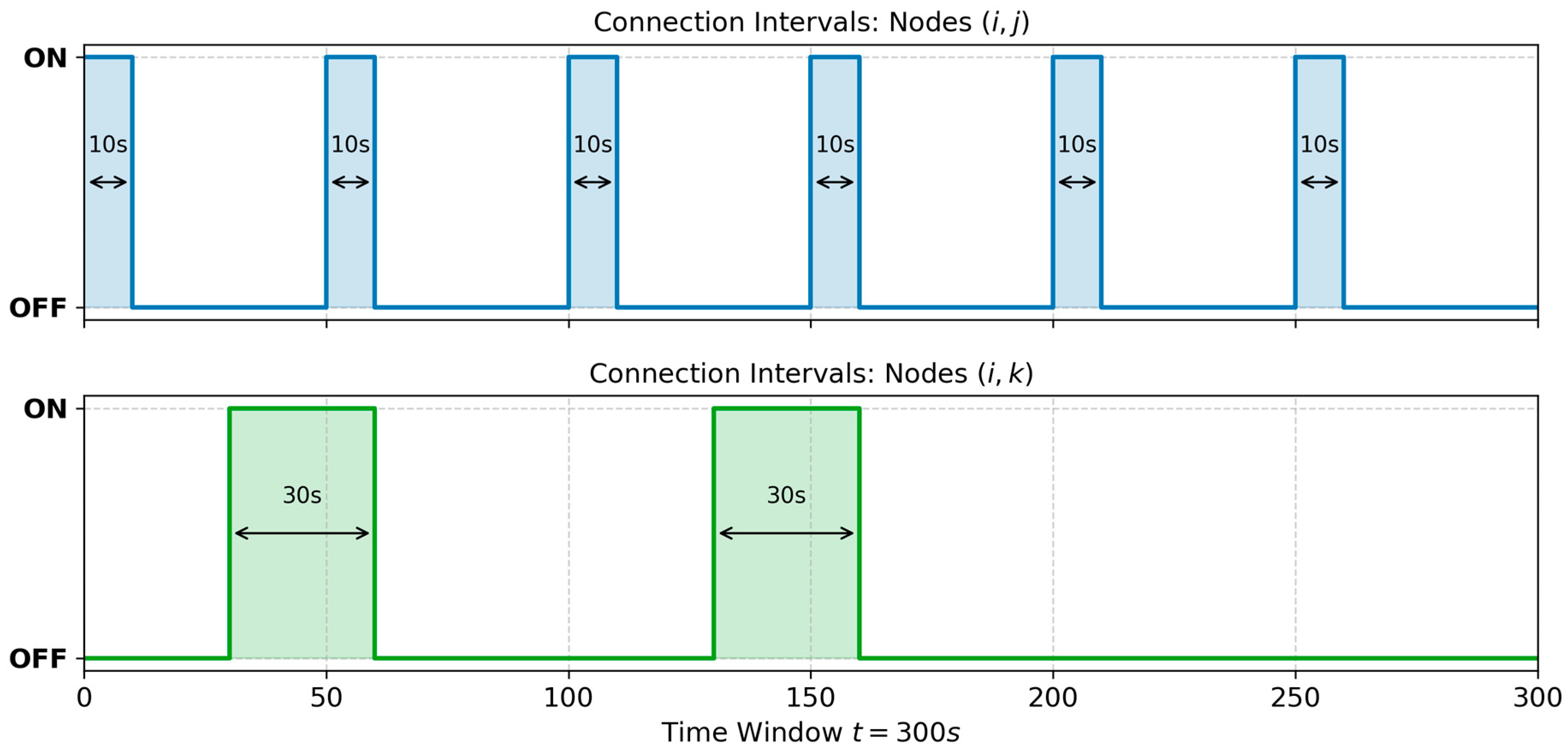
Figure 1. Illustrative example of connection intervals.
Electronics 15 02351 g001
Figure 2. Illustrative example of disconnection intervals.
Electronics 15 02351 g002
Figure 3. Topological representation of the simulation environments as rendered by the ONE simulator’s routing interface. The graphical outputs display the strictly navigable paths derived from OpenStreetMap (OSM) data for the Shortest Path Map-Based Movement model: (a) Downtown Helsinki (4.5 × 3.4 km); and (b) Metropolitan Manaus (35 × 35 km). Note that traditional cartographic elements (e.g., scale bars and compass roses) are inherently abstracted by the simulator’s internal relative coordinate system.
Electronics 15 02351 g003
Figure 4. Routing performance metrics in the dense pedestrian network (Helsinki) as a function of varying node density (125 to 1000 nodes). The panels detail: (a) Delivery Rate (%), (b) Average Latency (min), (c) Network Overhead, and (d) Total Energy Consumption (J). Data points represent the arithmetic mean of 15 independent simulation runs.
Electronics 15 02351 g004aElectronics 15 02351 g004b
Figure 5. Routing performance metrics in the dense pedestrian network (Helsinki) as a function of varying buffer size (2 to 16 MB). The panels detail: (a) Delivery Rate (%), (b) Average Latency (min), (c) Network Overhead, and (d) Total Energy Consumption (J). Data points represent the arithmetic mean of 15 independent simulation runs.
Electronics 15 02351 g005
Figure 6. Routing performance metrics in the dense pedestrian network (Helsinki) as a function of varying message TTL (15 to 120 min). The panels detail: (a) Delivery Rate (%), (b) Average Latency (min), (c) Network Overhead, and (d) Total Energy Consumption (J). Data points represent the arithmetic mean of 15 independent simulation runs.
Electronics 15 02351 g006
Figure 7. Routing performance metrics in the dense pedestrian network (Helsinki) as a function of varying message generation intervals (5 to 40 s). The panels detail: (a) Delivery Rate (%), (b) Average Latency (min), (c) Network Overhead, and (d) Total Energy Consumption (J). Data points represent the arithmetic mean of 15 independent simulation runs.
Electronics 15 02351 g007
Figure 8. Routing performance metrics in the sparse vehicular network (Manaus) as a function of varying node density (125 to 1000 nodes). The panels detail: (a) Delivery Rate (%), (b) Average Latency (min), (c) Network Overhead, and (d) Total Energy Consumption (J). Data points represent the arithmetic mean of 15 independent simulation runs.
Electronics 15 02351 g008aElectronics 15 02351 g008b
Figure 9. Routing performance metrics in the sparse vehicular network (Manaus) as a function of varying buffer sizes (10 to 80 MB). The panels detail: (a) Delivery Rate (%), (b) Average Latency (min), (c) Network Overhead, and (d) Total Energy Consumption (J). Data points represent the arithmetic mean of 15 independent simulation runs.
Electronics 15 02351 g009
Figure 10. Routing performance metrics in the sparse vehicular network (Manaus) as a function of varying message TTL (15 to 120 min). The panels detail: (a) Delivery Rate (%), (b) Average Latency (min), (c) Network Overhead, and (d) Total Energy Consumption (J). Data points represent the arithmetic mean of 15 independent simulation runs.
Electronics 15 02351 g010
Figure 11. Routing performance metrics in the sparse vehicular network (Manaus) as a function of varying message generation intervals (5 to 40 s). The panels detail: (a) Delivery Rate (%), (b) Average Latency (min), (c) Network Overhead, and (d) Total Energy Consumption (J). Data points represent the arithmetic mean of 15 independent simulation runs.
Electronics 15 02351 g011
Table 1. General simulation parameters for the evaluated scenarios.
ParameterScenario 1 (Helsinki)Scenario 2 (Manaus)
Map dimensions4.5 × 3.4 km35 × 35 km
Mobility modelShortest Path Map-BasedShortest Path Map-Based
Simulation duration12 h (43,200 s)15 h (54,000 s)
Node speed0.5 to 1.5 m/s30 to 60 km/h
Interface and rangeBluetooth LE (10 m)Wi-Fi 6 (100 m)
Transmission rate250 kBps25 MBps
Message size300 to 500 kB1 to 5 MB
TX/RX Power15.84 mW/10.89 mW640.5 mW/231.4 mW
Q-Learning Rate (α)0.30.3
Table 2. Default values adopted for the independent analysis variables.
Analysis VariableDefault Value
Number of nodes500 devices
Message Time-to-Live (TTL)60 min
Message generation interval15 s
Initial number of copies6 copies
Buffer size (Helsinki)5 MB
Buffer size (Manaus)50 MB
Disclaimer/Publisher’s Note: The statements, opinions and data contained in all publications are solely those of the individual author(s) and contributor(s) and not of MDPI and/or the editor(s). MDPI and/or the editor(s) disclaim responsibility for any injury to people or property resulting from any ideas, methods, instructions or products referred to in the content.