Path Loss Prediction in Dense WSN–IoT Networks with Machine Learning Techniques Across Diverse Terrains for Energy-Efficient Connectivity

Abstract

Accurate path loss prediction is essential for reliable and energy-efficient operation of dense Wireless Sensor Network–Internet of Things (WSN–IoT) systems, where radio transmission dominates node energy consumption and significantly impacts network lifetime. However, existing empirical or simulated models cannot achieve high prediction accuracy without explicitly linking statistical error metrics to system-level design parameters, thus limiting their practical interpretability in deployment scenarios. This work presents an extensive comparative evaluation among well-known propagation models versus machine learning regressors, and a lightweight convolutional neural network (CNN) for path loss prediction, using transmitter–receiver distance and carrier frequency as input features. A pairwise communication model is adopted to ensure consistent analysis across heterogeneous environments while preserving physical interpretability of the propagation process. Building upon this evaluation, a unified analytical framework is proposed that correlates path loss (PL) prediction accuracy to system-level metrics relevant to WSN–IoT design. Moreover, in this work we apply the Root Mean Square Error (RMSE) of the best-performing model as an empirical estimate of the shadowing standard deviation, under standard statistical assumptions, thereby allowing its direct use in link budget and fade margin calculations. Extensive experimental results across five heterogeneous wireless link datasets demonstrate that improved prediction accuracy leads to reduced transmission power requirements, lower energy consumption, enhanced communication reliability, and extended node lifetime.

1. Introduction

Designing dense Wireless Sensor Network–Internet of Things (WSN–IoT) systems that simultaneously achieve high reliability and energy efficiency critically depends on the accurate characterization of large-scale propagation effects, as path loss directly determines link quality, communication reliability, and node energy consumption [1,2,3]. In battery-powered deployments, radio transmission constitutes the dominant component of energy expenditure, making propagation-aware system design essential for extending network lifetime and ensuring sustainable operation [4,5,6]. Consequently, fundamental design tasks such as link budget analysis, transmit power estimation, and reliability provisioning must explicitly account for environmental propagation mechanisms, including multipath propagation, shadowing, clutter, vegetation, and non-line-of-sight conditions, which are particularly pronounced in dense and heterogeneous deployment scenarios [7].

Classical empirical propagation models, including free-space, log-distance, and COST-family formulations, remain widely adopted due to their analytical simplicity and low computational complexity. However, their limited ability to capture environment-specific variability and complex propagation phenomena often leads to inaccurate path loss estimation, resulting in suboptimal fade margin selection, degraded communication reliability, and inefficient energy utilization [7]. To address these limitations, data-driven approaches based on machine learning (ML) and deep learning (DL) have been increasingly investigated for path loss prediction, demonstrating the ability to model nonlinear propagation behavior directly from measurement data [8,9,10].

A broad range of ML-based techniques—including neural network ensembles, hybrid regression–classification models, and other data-driven approaches—have demonstrated improved predictive accuracy in several studies [11,12,13,14]. Furthermore, uncertainty-aware learning frameworks have been introduced to enhance robustness under stochastic channel conditions by explicitly modeling predictive uncertainty [15,16]. Comparative analyses across indoor, outdoor, and heterogeneous scenarios further confirm the effectiveness of ML-based models over classical approaches in complex environments [17]. Recent survey studies have highlighted the increasing heterogeneity and complexity of propagation environments across diverse wireless communication scenarios, emphasizing the need for accurate and generalizable path loss modeling approaches [18]. In parallel, node lifetime estimation in WSN–IoT systems has been traditionally studied using duty-cycle-based models, residual energy tracking, and traffic-aware approaches that abstract away propagation effects. While these methods are effective in capturing energy consumption patterns, they typically decouple energy modeling from channel variability and do not explicitly account for propagation-induced transmission power variations.

The development and evaluation in such data-driven frameworks require robust statistical validation methodologies to ensure generalization capability and prevent overfitting. In this context, cross-validation techniques provide a principled approach for model assessment and selection [19,20]. Within this framework, widely adopted ML algorithms such as random forests, gradient boosting, XGBoost, and extremely randomized trees provide strong nonlinear modeling capabilities and have been extensively validated in predictive modeling applications [21,22,23,24]. In parallel, energy-aware operation remains a critical design constraint in WSN–IoT systems, where communication efficiency directly impacts battery lifetime and long-term system sustainability [25,26,27].

Despite these advances, the majority of existing studies primarily focus on statistical accuracy metrics, such as RMSE, MAE, and R² without explicitly linking prediction performance to system-level design parameters through a consistent and formally defined transformation process, including link budgeting, fade margin determination, transmission power estimation, and network lifetime optimization. More importantly, these approaches do not provide a formally defined mechanism that translates prediction accuracy into operational communication system parameters. In particular, no explicit and reproducible mapping is established between statistical error metrics (such as RMSE) and key system-level design quantities, including fade margin, required transmission power, and node lifetime. This limitation is particularly critical in WSN–IoT systems, where energy-aware operation is tightly coupled with propagation uncertainty and channel variability [5,6]. Additionally, existing node lifetime estimation approaches are often developed independently of propagation modeling, resulting in a lack of explicit linkage between channel uncertainty, transmission power requirements, and energy consumption dynamics. As a result, existing approaches typically treat propagation modeling, prediction accuracy, and energy-aware system design as loosely coupled components rather than as part of a unified and explicitly defined analytical framework.

To address this gap, this work proposes a deployment-oriented framework that establishes a unified and statistically grounded transformation framework, within which classical propagation models, multiple ML regressors, and a lightweight Convolutional Neural Network (CNN) are systematically evaluated under consistent experimental conditions. The framework operates under standard large-scale propagation assumptions, including log-normal shadowing and approximately zero-mean residual errors, which are well-established in propagation theory [1,2]. RMSE can be interpreted, under appropriate statistical assumptions, as an empirical indicator of prediction dispersion consistent with propagation variability, enabling a practical—though not strictly physical—mapping between prediction accuracy and system-level design parameters, such as fade margin and required transmission power.

The novelty of this work lies in the formalization of an explicit propagation-to-system mapping that bridges data-driven path loss prediction and communication system design metrics within a unified analytical framework. In particular, rather than focusing exclusively on improving prediction accuracy, the proposed approach introduces a structured and reproducible transformation process in which prediction error (RMSE) is statistically interpreted as a proxy for channel variability under explicit conditions, subsequently mapped to fade margin through reliability constraints, and finally incorporated into link budget analysis and energy-aware network design. This formulation enables a direct and operational linkage between data-driven modeling outputs and system-level performance metrics, allowing a consistent assessment of how improvements in prediction accuracy influence transmission power requirements, communication reliability, and node lifetime in heterogeneous deployment scenarios. In this context, the proposed framework is not intended to replace existing energy or lifetime models, but rather to extend them through a propagation-aware and statistically grounded integration mechanism. To the best of our knowledge, no prior work provides an explicit and reproducible transformation from prediction error metrics to system-level design parameters within a unified analytical framework. Accordingly, the contribution of this work is centered on uncertainty propagation and system-level analytical integration rather than on the development of a new standalone propagation or energy model.

The proposed methodology is validated across multiple heterogeneous wireless link datasets, ensuring that environment-specific variability is captured while maintaining methodological consistency. The experimental results demonstrate that improved prediction accuracy is systematically associated with reduced transmission power requirements, enhanced communication reliability, and extended network lifetime under identical hardware constraints. Unlike existing approaches, the proposed framework explicitly bridges the gap between prediction accuracy and system-level design, providing a practical and technology-agnostic tool for energy-aware and reliability-aware WSN–IoT system design.

The main contributions of this work are summarized as follows:

• Formalization of a propagation-to-system mapping that translates statistical prediction error (RMSE) into channel variability under explicit statistical assumptions, enabling its integration into communication system design.
• Development of a unified and reproducible transformation process that links path loss prediction, fade margin estimation, link budget analysis, and node lifetime evaluation within a consistent analytical framework.
• Establishment of a reliability-aware interpretation of machine learning performance, where prediction accuracy is directly connected to communication reliability and transmission power requirements.
• Comprehensive cross-dataset validation demonstrating that improvements in predictive accuracy systematically translate into measurable gains in energy efficiency and network lifetime under identical system constraints.
• Provision of a technology-agnostic and deployment-oriented framework that bridges the gap between data-driven propagation modeling and practical wireless system design.

The remainder of this article is organized as follows. Section 2 reviews the related work and motivation. Section 3 details the proposed methodology. Section 4 presents the comparative results and discusses the practical implications of the findings for dense IoT deployments, and Section 5 concludes the paper.

2. Related Work and Motivation

Recent studies on path loss modeling in WSN–IoT environments have increasingly relied on heterogeneous datasets collected from diverse propagation scenarios in order to capture variability across environments, frequencies, and deployment conditions. Such datasets highlight the limitations of classical empirical models, which are typically derived under simplified assumptions and therefore exhibit reduced adaptability when applied to cross-environment scenarios [28]. As a result, their predictive performance often degrades when evaluated beyond the conditions for which they were originally calibrated.

To address these limitations, machine learning regressors have been widely investigated for path loss prediction using heterogeneous datasets, demonstrating improved ability to approximate nonlinear propagation behavior directly from measurement data [29]. These models are commonly evaluated across multiple datasets to assess their robustness and generalization capability under varying environmental conditions. In parallel, convolutional neural network (CNN) architectures have been introduced as lightweight deep learning models capable of learning structured representations from input features such as transmitter–receiver distance and frequency. When trained on heterogeneous datasets, CNN-based approaches have shown competitive performance compared to conventional regressors, particularly in scenarios involving complex propagation effects.

In addition, hybrid regression approaches that combine different learning strategies have been proposed to further enhance prediction accuracy by leveraging complementary modeling characteristics [30]. These methods aim to improve robustness across heterogeneous datasets by adapting to variations in propagation regimes. Kernel-based regressors, such as support vector regression (SVR), are also commonly used as reference models due to their strong theoretical foundation and ability to handle nonlinear relationships in high-dimensional feature spaces [31]. Across the literature, such methods are typically benchmarked on heterogeneous datasets to evaluate their comparative predictive performance.

Despite the extensive use of heterogeneous datasets and a variety of machine learning regressors and CNN-based models, existing work remains predominantly focused on statistical performance evaluation. In particular, model comparison is usually conducted using error metrics without explicitly interpreting how prediction accuracy relates to propagation uncertainty or system-level design requirements [29,30]. This is consistent with broader trends in the literature, where path loss prediction studies emphasize accuracy improvements but do not establish a direct mapping between modeling errors and practical deployment parameters such as fade margin selection, transmission power allocation, and reliability constraints [28,31]. Consequently, although heterogeneous datasets and advanced learning models improve predictive capability, their evaluation is largely limited to benchmarking tasks, without providing direct insight into their implications for communication system design.

Recent advances in adaptive and learning-based frameworks further illustrate the increasing integration of data-driven intelligence with system-level objectives. For example, the work in [32] proposes an autonomous online learning methodology capable of generating structured tutorials, highlighting the role of continuous learning and adaptive knowledge extraction in dynamic environments. Although developed in a different application domain, such approaches reflect a broader trend toward self-adaptive learning systems.

In parallel, reinforcement learning (RL) techniques have been explored for energy-aware communication optimization in resource-constrained wireless systems. The study in [33] introduces a deep reinforcement learning (DRL)-based framework for underwater acoustic sensor networks (UASNs), where coding strategies are dynamically adapted to channel conditions and energy constraints in order to improve reliability and energy efficiency.

These approaches focus primarily on adaptive decision-making and control policies. In contrast, the framework proposed in this work is deployment-oriented and emphasizes a statistically grounded transformation pipeline that explicitly links prediction uncertainty to communication system design parameters, including fade margin, transmission power, and node lifetime. As such, it provides a complementary perspective by enabling a reproducible and model-agnostic integration of propagation modeling with system-level design.

This observation motivates the need for modeling and evaluation approaches that not only assess predictive performance across heterogeneous datasets but also establish an explicit and consistent linkage between statistical model accuracy and communication system design parameters through a unified analytical framework, rather than treating these aspects independently as in most existing studies.

3. Proposed Methodology

3.1. Communication Model

To analyze wireless communication behavior in dense WSN-IοΤ deployments, a system representation based on a pair of communicating transceivers is adopted. Although large-scale sensor networks consist of many spatially distributed nodes, communication fundamentally occurs through individual wireless links established between neighboring nodes. Modeling the interaction between two transceivers therefore provides a practical abstraction for studying link-level propagation characteristics and enables the integration of prediction accuracy into energy-aware link budget analysis and node lifetime estimation.

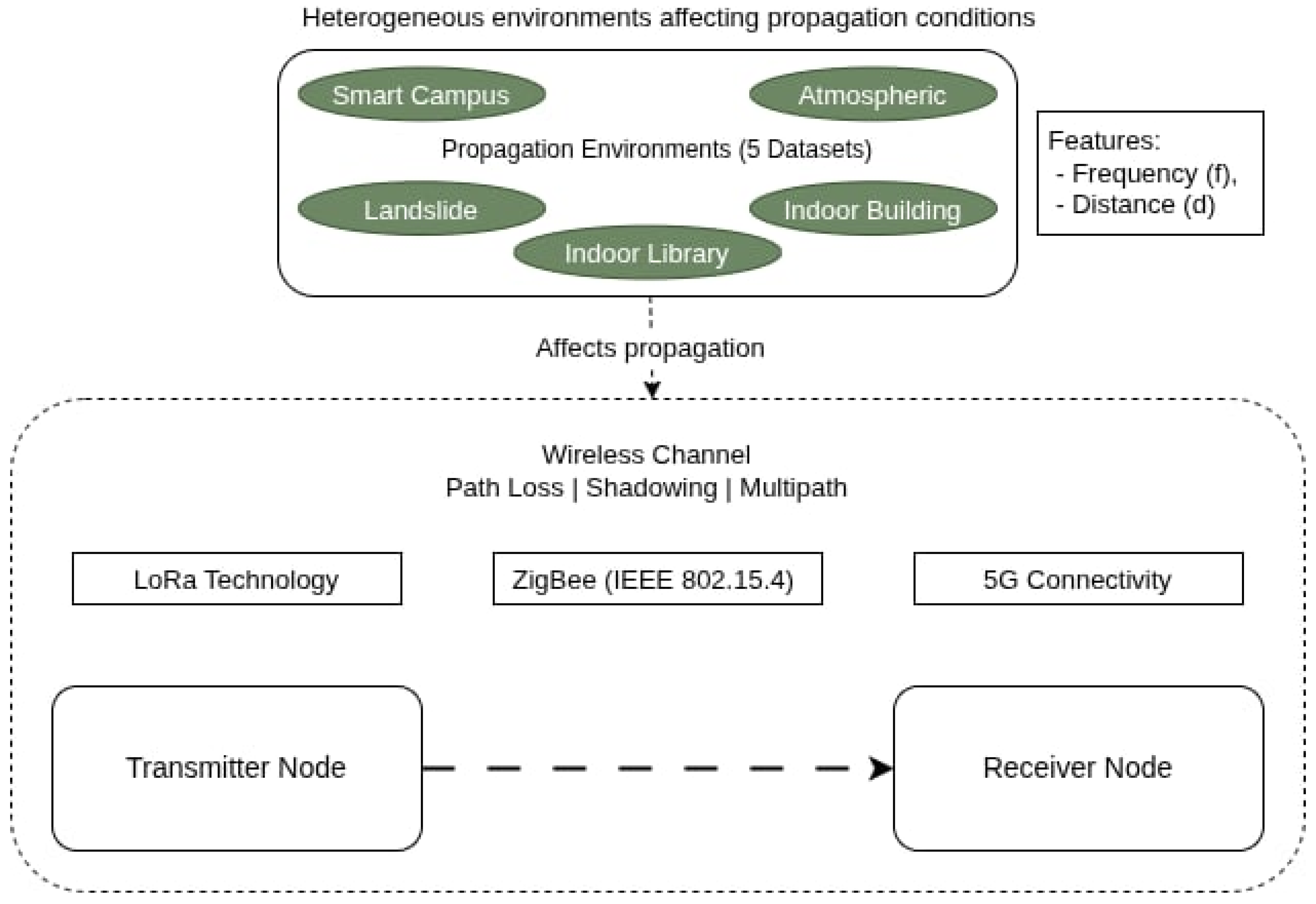
By parameterizing the transmitter–receiver distance and the operating frequency, this pairwise representation captures the dominant large-scale factors affecting signal propagation and path loss. These parameters remain fundamental for wireless link quality and network planning [1,2]. The transmitter–receiver distance is treated as either a measurable or design parameter depending on the deployment scenario, allowing the framework to remain applicable across both planned and data-driven network configurations. In dense and randomly deployed networks, each data transmission corresponds to a point-to-point interaction between neighboring nodes during data forwarding or multi-hop routing. Consequently, the behavior of arbitrary communication links can be approximated using this model, enabling scalable analysis of large-scale WSN and IoT infrastructures [1,2], as illustrated in Figure 1.

Each node integrates sensing, processing, and radio communication capabilities and may support wireless technologies commonly used in IoT systems, such as ZigBee based on the IEEE 802.15.4 standard [34] (IEEE Standard 802.15.4; IEEE Standard for Low-Rate Wireless Networks. IEEE: New York, NY, USA, 2020) for short-range energy-efficient communication, LoRa for long-range connectivity in geographically dispersed or obstacle-rich environments, and 5G connectivity where infrastructure support and higher data rates are available. The wireless channel between nodes is affected by attenuation, shadowing, and multipath propagation. These effects vary with terrain morphology and environmental conditions, leading to different path loss characteristics across deployment scenarios [1,2].

3.2. Datasets

To capture diverse propagation conditions, a collection of publicly available datasets from both peer-reviewed studies and open repositories covering atmospheric, smart campus, indoor building, indoor library, and landslide scenarios is employed for training and evaluation of machine learning models for path loss prediction. All models use transmitter–receiver distance and carrier frequency as input features to ensure a consistent and comparable feature space across datasets. The datasets include both empirical measurements and synthetic channel data generated using the NYUSIM channel simulator. The synthetic dataset is used to emulate high-frequency propagation conditions (mmWave) that are difficult to capture through large-scale measurements, while energy-aware analysis is interpreted in a comparative and scenario-based manner rather than as a hardware-specific deployment prediction. The synthetic dataset spans sub-GHz to millimeter-wave frequencies and includes multiple propagation environments characterized by varying shadowing levels, multipath effects, and line-of-sight (LOS/NLOS) conditions [35]. Combining simulated and measured datasets improves coverage of propagation regimes and supports evaluation of model generalization across heterogeneous environments. To address potential domain shift between heterogeneous real-world and synthetic datasets, a dataset-isolated evaluation strategy is adopted. Specifically, no joint training across datasets is performed. All models are trained, validated, and evaluated independently within each dataset using a consistent cross-validation protocol, without any cross-dataset data sharing or joint optimization. This design ensures that no information leakage occurs between domains and that each dataset is treated as a distinct propagation domain with its own underlying statistical characteristics. As a result, biases arising from distribution mismatch between simulated and real-world data are inherently mitigated by the evaluation design. Consequently, performance analysis focuses strictly on within-dataset comparisons rather than direct comparison of absolute metrics across datasets, enabling a controlled and fair assessment of model behavior under heterogeneous but internally consistent propagation conditions. It is important to clarify that the cross-band evaluation is conducted at the level of large-scale propagation modeling, where path loss is represented in the logarithmic (dB) domain as a function of distance and frequency. Under this abstraction, different frequency regimes share a common statistical representation based on distance-dependent attenuation and log-normal variability, allowing consistent evaluation within the proposed framework without implying equivalence of the underlying microscopic fading mechanisms.

The synthetic dataset (NYUSIM) is included in a complementary manner to extend coverage to high-frequency propagation regimes, and is not intended to substitute real-world measurements, thereby avoiding cross-domain interference that could arise from distribution mismatch between simulated and real-world propagation conditions.

The evaluated models include classical propagation models [1,2], multiple machine learning regressors [10,17], ensemble methods [21,22,23,24], and deep learning architectures, including CNNs [9]. These models are selected to capture nonlinear and environment-dependent propagation behaviors.

The selected datasets were chosen to ensure a comprehensive evaluation of model performance across heterogeneous and realistic propagation conditions. Specifically, they cover diverse environments, including indoor (Indoor Building, Indoor Library), outdoor urban (Smart Campus), terrain-affected (Landslide), and high-frequency scenarios (Atmospheric dataset generated using the NYUSIM channel simulator). This selection enables the analysis of key propagation effects such as multipath, shadowing, and LOS/NLOS conditions. In addition, the datasets span multiple frequency bands from sub-GHz to millimeter-wave ranges, and include both real-world measurements and synthetically generated data, ensuring coverage of different propagation regimes while maintaining physical realism. Overall, this strategy was adopted to assess the generalization capability and robustness of the models across heterogeneous deployment scenarios rather than optimizing performance for a specific environment. In addition to model evaluation, the selected datasets enable system-level analysis by providing representative path loss distributions that can be directly mapped to link budget requirements, transmission power estimation, and energy-aware node lifetime analysis.

The datasets employed in this study represent a wide range of propagation environments relevant to heterogeneous wireless systems, including WSN, IoT, short-range wireless, and cellular communication scenarios. They include a millimeter-wave dataset generated using the NYUSIM channel simulator covering Urban Microcell scenarios at 7.125 GHz, 24.25 GHz, 52.60 GHz, and 71 GHz [35]; a smart campus dataset collected at Covenant University at 1800 MHz with 3617 measured samples obtained via drive tests [36]; two indoor datasets, one from a multi-floor academic building using LoRa in the sub-GHz band with structural descriptors such as number of floors and walls [37], and another from a 3.5 GHz measurement campaign in a large library environment with dense structural variability [38]; and a terrain-affected dataset from a landslide-prone area in Thailand at 2400 MHz with transmitter–receiver distances ranging from 0.5 m to 50 m and repeated measurements to mitigate small-scale fading effects. The authors provide additional path loss measurement and simulation data as supplemental material to the article by [39]. Each dataset implicitly corresponds to a different communication technology and deployment scenario (e.g., sub-GHz LPWAN, short-range wireless, WiFi, and cellular systems), which justifies the use of technology-specific transmission power consumption models in the subsequent energy-aware analysis. This dataset-isolated strategy ensures evaluation within statistically consistent domains without cross-domain generalization.

Together, these datasets provide a comprehensive benchmark for evaluating model generalization across diverse propagation regimes while supporting deployment-level tasks such as transmission power planning, fade margin estimation, energy consumption analysis, and node lifetime prediction under realistic and heterogeneous conditions. Although some datasets contain additional environmental descriptors, these are excluded from the learning process to maintain a unified feature space and ensure fair cross-dataset comparability without dataset-specific tuning. This design choice ensures that the learned models remain agnostic to environment-specific descriptors, allowing the derived performance and uncertainty metrics (e.g., RMSE) to be consistently interpreted across datasets for subsequent system-level analysis.

To ensure methodological rigor, reproducibility, and consistency within the proposed unified framework, a unified experimental pipeline is adopted across all datasets. The feature space is restricted to transmitter–receiver distance (d) and carrier frequency (f), and all distance values are consistently converted to the appropriate units required by each propagation model implementation. A standardized preprocessing procedure is applied [20], without dataset-specific calibration of analytical models, preserving their intrinsic formulations. Model evaluation is conducted using 5-fold cross-validation with data shuffling and a fixed random seed [19]. Performance is assessed using Mean Absolute Error (MAE), RMSE, and the coefficient of determination (R²). RMSE is additionally used as a proxy for prediction uncertainty and, under explicitly validated statistical conditions, as an empirical indicator of dispersion consistent with shadowing variability, enabling its subsequent use in fade margin estimation and energy-aware link budget analysis [1,2,15,16,19,20]. All experiments are implemented within a consistent pipeline to ensure fair benchmarking across model classes. The use of a unified preprocessing and evaluation pipeline ensures that performance differences reflect propagation characteristics rather than methodological inconsistencies, reducing potential bias when analyzing heterogeneous datasets. The implementation tool was Python 3.12.10 using NumPy 2.1.3, Pandas 2.2.3, SciPy 1.15.2, and scikit-learn 1.6.1 for data processing and classical machine learning models. Deep learning models were developed using TensorFlow 2.19.0, while XGBoost 3.1.1 was used for gradient boosting experiments. Visualization was performed using Matplotlib 3.10.1 and Seaborn 0.13.2. This software stack ensures reproducibility and consistency across all experiments.”

Summary statistics for each dataset, including number of samples, distance and frequency ranges, and environment type, are provided in

Table 1. Summary Statistics for Path Loss Datasets.

Dataset	Number of Samples	Distance Range (m)	Frequency Range (MHz)	Technology Type
Atmospheric	2835	10–2000	7125–71,000	mmWave Cellular/5G
Smart Campus	3617	1–1135	1800	WiFi/Zigbee
Indoor Building	1317	6–106	868.1–868.5	LoRa/LPWAN
Indoor Library	343	14–27	3500	WiFi
Landslide	100	1–50	2400	Zigbee/ISM

.

For each dataset, the regression task is defined using a constrained feature space consisting exclusively of transmitter–receiver distance d (meters) and carrier frequency f (MHz) [1,2]:

$$x=\left[d,f\right]$$

The target variable is the measured path loss in decibels [7]:

$$y=P{L}_{\mathrm{dB}}$$

All datasets [32,33,35,36,37] were processed using a unified preprocessing pipeline to ensure methodological consistency. Column names were standardized, and only the universally available features—distance, frequency, and path loss—were retained. Samples with invalid entries (non-positive distance or frequency) or missing values were removed [20]. No dataset-specific feature engineering or environment-dependent adjustments were introduced, ensuring a fair benchmarking procedure across heterogeneous propagation scenarios [19,20]. The large-scale propagation behavior between a transmitter and a receiver is described by the path loss PL(d,f), where d denotes the transmitter–receiver distance in meters and f the carrier frequency in MHz. The received power is defined as:

$$P_{rx}=P_{tx}-PL\left(d,f\right)$$

(1)

where antenna gains and hardware losses are incorporated into the effective path loss term [1,2]. This formulation provides the foundation for the subsequent integration of propagation modeling with link budget analysis and energy-aware system design, where predicted path loss values are translated into transmission power requirements and node lifetime estimates under realistic deployment assumptions.

The corresponding publicly accessible repositories, DOI references, and dataset resources associated with References [35,36,37,38,39] are explicitly provided in the Data Availability Statement to ensure transparency and reproducibility.

3.3. Propagation Models

To establish a robust comparative baseline for wireless channel characterization, a set of widely adopted empirical and semi-empirical propagation models is implemented, namely the Free Space Path Loss (FSPL), Okumura–Hata, COST-231 Hata, Log-Distance, Egli, and ITU indoor models. The selection of these models is guided by the heterogeneous nature of the datasets employed in this study, which encompass indoor, outdoor urban, terrain-affected, and high-frequency propagation scenarios. Accordingly, the chosen models collectively cover the corresponding propagation regimes: indoor-oriented formulations such as the ITU model are aligned with indoor datasets, urban macrocell models such as Okumura–Hata and COST-231 are representative of outdoor urban environments, general-purpose models such as FSPL and Log-Distance provide baseline formulations applicable across conditions, while terrain-sensitive models such as Egli capture irregular propagation effects relevant to environments with non-uniform terrain characteristics. This alignment ensures that the evaluation framework reflects realistic deployment conditions and enables a consistent assessment of both environment-specific applicability and cross-environment generalization capability. These models are extensively used in wireless communication system design and are applicable across heterogeneous environments, including rural, suburban, urban, and indoor scenarios [28]. Consistent parameterization is applied across all models to ensure comparability, with frequency expressed in MHz and distance converted to kilometers where required by specific formulations, while antenna heights are fixed at representative values of 30 m for the base station and 1.5 m for the receiver.

The parameters used in the propagation models are summarized in

Table 2. Parameters used in propagation models.

Symbol	Description	Units
PL	Path Loss	dB
f	Operating frequency	MHz
d	Distance between transmitter and receiver	m or Km
ht	Transmitting antenna height	m
hr	Receiving antenna height	m

.

The FSPL model provides a theoretical lower bound for signal attenuation under ideal Line-of-Sight (LoS) conditions:

$$PL\left(d,f\right)=20lo{g}_{10}\left(d\right)+20lo{g}_{10}\left(f\right)+32.44$$

(2)

where d is the distance in kilometers and f is the operating frequency in MHz.

The Okumura–Hata model is an empirical formulation derived from extensive field measurements:

$$PL=69.55+26.16{log}_{10}\left(f\right)-13.82{log}_{10}\left(h_t\right)-a\left(h_r\right)+\left(44.9-6.55{log}_{10}\left(h_t\right)\right){log}_{10}\left(d\right)$$

(3)

where d is in kilometers and $a\left(h_m\right)$ represents the mobile antenna height correction factor.

The COST-231 Hata model extends the Okumura–Hata formulation to higher frequency bands (1500–2000 MHz):

$$PL=46.3+33.9{log}_{10}\left(f\right)-13.82{log}_{10}\left(h_t\right)-a\left(h_r\right)+\left(44.9-6.55{log}_{10}\left(h_t\right)\right){log}_{10}\left(d\right)+C$$

(4)

where C is an environmental constant (0 dB for suburban and medium-sized cities, and 3 dB for metropolitan areas).

The Log-Distance model generalizes FSPL by introducing a path loss exponent:

$$PL\left(d\right)=PL\left(d_0\right)+10n{log}_{10}\left({\displaystyle \frac{d}{d_0}}\right)$$

(5)

where n denotes the path loss exponent and depends on the propagation environment and d₀ denotes the reference distance (typically 1 m).

The Egli model accounts for antenna heights and partial obstruction:

$$PL=20{log}_{10}\left(f\right)+40{log}_{10}\left(d\right)-20{log}_{10}\left(h_t\right)-20{log}_{10}\left(h_r\right)+117$$

(6)

where h_t and h_r denote the transmitting and receiving antenna heights, respectively. This notation is consistent with the global variable definitions provided in Table 2.

The ITU indoor model incorporates structural attenuation effects:

$$PL\left(d,f\right)=20{log}_{10}\left(f\right)+N{log}_{10}\left(d\right)+L_f\left(n\right)-28$$

(7)

where N is the distance power loss coefficient and $L_f\left(n\right)$ represents floor penetration loss.

These models collectively provide a comprehensive baseline for evaluating propagation behavior across diverse environments [28].

3.4. Machine Learning Models

To model the nonlinear relationship between propagation parameters and measured path loss, several machine learning regression algorithms are employed, including ensemble methods, kernel-based models, and neural networks [17,40]. The selection of these models is guided by the need to provide a comprehensive set of widely adopted regression approaches capable of capturing nonlinear propagation behavior across heterogeneous datasets. In particular, ensemble methods such as Random Forests [21], Gradient Boosting [22], XGBoost [23], and Extremely Randomized Trees [24] are included due to their strong ability to improve generalization through the aggregation of multiple decision trees and their robustness to noise and dataset variability, as established in classical classification and regression tree (CART) methodology [41]. A Decision Tree Regressor is also considered as a baseline model for reference.

Support Vector Regression (SVR) with an RBF kernel is employed to capture nonlinear relationships in high-dimensional feature spaces [31], while a Multi-Layer Perceptron (MLP) trained via backpropagation [42] is used as a representative feedforward neural network model capable of approximating complex mappings between input features and path loss. In addition, CNN architectures have shown competitive performance in specific scenarios [9,43]. The CNN configuration (layers, epochs, optimizer, and other hyperparameters) was selected through automated hyperparameter tuning to ensure fair and reproducible performance across datasets, following the experimental setup in [43]. The inclusion of these models ensures coverage of different regression paradigms, enabling a consistent and fair evaluation of their predictive performance and generalization capability across heterogeneous propagation scenarios.

All models use two input features (distance and frequency) to predict path loss in dB. Feature standardization is applied to ensure stable convergence. Model evaluation is performed using 5-fold cross-validation [19], and performance is assessed using MAE, RMSE, and R².

Residuals are further analyzed using the Shapiro–Wilk test [44] to assess their statistical distribution. RMSE is interpreted as a practical measure of prediction dispersion and, under approximately Gaussian residual conditions, as an estimator of shadowing variability. This interpretation is applied cautiously in cases where the Gaussian assumption does not strictly hold.

To further enhance reproducibility and methodological transparency, the hyperparameter configurations of the implemented machine learning and deep learning models, together with the preprocessing, cross-validation, and statistical evaluation settings adopted throughout the experimental pipeline, are summarized in Appendix A (

Table A1. Hyperparameter settings used for ML and DL regression models for PL prediction.

Model	Hyperparameters	Values
Random Forest Regressor	Number of Trees (n_estimators)	150
	Random State	42
XGBoost Regressor	Number of Trees (n_estimators)	200
	Learning Rate	0.05
	Maximum Depth (max_depth)	6
Gradient Boosting Regressor	Number of Trees (n_estimators)	200
	Learning Rate	0.05
Extra Trees Regressor	Number of Trees (n_estimators)	200
	Random State	42
Decision Tree Regressor	Random State	42
Support Vector Regression (SVR)	Kernel	RBF
	Regularization Parameter (C)	20
	Gamma	scale
Multi-Layer Perceptron Regressor	Hidden Layers	(128, 64)
	Activation Function	ReLU
	Maximum Iterations (max_iter)	1000
Convolutional Neural Network (CNN)	Convolution Filters	32
	Kernel Size	(1 × 2)
	Activation Function	ReLU
	Dropout Rate	0.2
	Dense Layer Neurons	64
	Output Neurons	1
	Optimizer	Adam
	Loss Function	Mean Squared Error (MSE)
	Epochs	200
	Batch Size	32
	Validation Split	0.2
	Early Stopping Patience	15
	Restore Best Weights	True

and

Table A2. Parameter settings used for Cross-validation, preprocessing, and statistical evaluation.

Parameter	Value
Cross-Validation Strategy	5-Fold Cross Validation
Shuffle	True
Random Seed	42
Feature Scaling	StandardScaler
Test Split Ratio	20%
CNN Internal Validation	Validation Split (0.2)
Early Stopping Criterion	Validation Loss
Evaluation Metrics	MAE, RMSE, R2
Statistical Validation	Shapiro–Wilk Normality Test
Confidence Level	95%
Energy Overhead Factor	1.35
Battery Derating Factor	0.70

).

3.5. Node Lifetime Estimation

Based on the developed modeling and evaluation pipeline, the framework translates the obtained path loss predictions into system-level operational metrics by linking them to transmission power requirements and energy usage in battery-constrained WSN–IoT nodes. The estimated path loss is integrated within a link budget formulation to derive the minimum transmission power required for reliable communication, directly affecting per-transmission energy expenditure and, consequently, the expected node lifetime. It is important to clarify that the proposed framework does not perform power control or dynamic transmission policy optimization. Instead, it serves as a recommendation-oriented framework that translates link budget requirements into transmission power levels, intended for system-level design guidance rather than real-time control. To ensure reproducibility and consistency with established energy-aware modeling approaches for wireless sensor networks, all assumptions and parameters used in the proposed framework are explicitly defined and grounded in prior literature on WSN energy consumption and communication system design [4,5,6,25,26,27]. The assumptions and parameter values are displayed in

Table 3. Global assumptions of the energy-aware model.

Parameter	Value	Description	Justification
Energy overhead factor (koh)	1.35	Includes DC–DC, MCU, protocol overhead	[4,5,6]
Battery derating factor	0.70	Effective usable battery capacity	[5,25]
Reliability target	95%	Target link availability	[1,2]
Fade margin factor	1.65	z-score for 95% reliability	[1,2]
Base path loss	Median (PL)	dataset-derived robust estimator	[1,2]
Lifetime cap	10 years	Practical IoT deployment limit	[5,6]

. It is emphasized that the contribution of this work does not lie in the individual formulation of these components, which are well established in the literature, but in their integration through a structured and statistically grounded transformation process that enables consistent propagation of prediction uncertainty into system-level performance metrics.

The considered network operation follows typical WSN–IoT behavior, where nodes transmit periodically and remain in low-power sleep states between transmissions [4,6,25]. The device and communication parameters are selected to reflect realistic operating conditions reported in WSN and IoT deployments and are aligned with the characteristics of the datasets and their corresponding application scenarios [4,5,25,39]. These parameters are summarized in

Table 4. Scenario-specific device and communication parameters.

Dataset	Interval (s)	Battery (mAh)	Packet (Bytes)	Bitrate (kbps)	Sleep Current (mA)	Rx Sensitivity (dBm)
Landslide	300	2500	128	250	0.008	−95
Smart Campus	600	2600	128	250	0.02	−100
Indoor Building	900	2400	64	5.4	0.006	−137
Indoor Library	600	2500	128	500	0.03	−90
Atmospheric	900	3000	64	1000	0.08	−78

.

These parameters are not tied to a specific hardware platform but represent typical configurations reported in the literature for comparable deployment scenarios.

Given that wireless transmission represents the dominant component of energy consumption in such systems [4,5,6,26,27], accurate estimation of transmission power becomes critical for achieving energy-efficient operation. For each dataset, the model with the lowest RMSE is selected as the best-performing model for reliability-aware evaluation. In this context, this selection defines the reference model for generating power level suggestions rather than implying any control mechanism. Consequently, the overall framework remains recommendation-oriented rather than selection-driven. Furthermore, RMSE is interpreted as a proxy for prediction uncertainty and, under explicitly validated statistical conditions, as an approximate indicator of dispersion consistent with shadowing variability. This interpretation is conditional and does not imply that residuals exclusively represent physical channel effects.

3.5.1. Prediction Error, Channel Variability, and Fade Margin

Propagation model accuracy is evaluated using the RMSE calculated on an independent test dataset. For $N$ samples with measured path loss $P{L}_i^{meas}$ and predicted values $P{L}_i^{pred}$, the RMSE is defined as: [19].

$$RMSE=\sqrt{\left(\left({\displaystyle \frac{1}{N}}\right){\sum }_{i=1}^N{\left(P{L}_i^{pred}-P{L}_i^{meas}\right)}^2\right)}$$

(8)

Large-scale propagation effects are commonly modeled using the log-normal shadowing model, where path loss consists of a deterministic component plus a Gaussian random variable in the logarithmic (dB) domain with standard deviation $\sigma$ [1,2].

Let the prediction residual be,

$${ϵ}_i=P{L}_i^{meas}-P{L}_i^{pred}$$

(9)

The Mean Squared Error (MSE) of the residual distribution is [1,2].

$$MSE={\sigma }^2+bia{s}^2$$

(10)

where ${\sigma }^2$ denotes the variance of the residuals and $bias=E\left[ϵ\right]$ denotes the mean residual. The bias corresponds to the mean value of the residuals and quantifies systematic over- or under-estimation, while σ² represents the variance of the residuals and is associated with the shadowing component of large-scale propagation.

The proposed methodology does not assume a direct equivalence between RMSE and the shadowing standard deviation (σ), but instead evaluates whether RMSE can serve as an approximate estimator of dispersion consistent with shadowing variability under explicitly defined statistical conditions. First, the absence of systematic error is assessed by testing whether the residual mean is statistically indistinguishable from zero (bias ≈ 0) using a two-sided hypothesis test at a predefined significance level (e.g., α = 0.05), i.e., H₀: μ = 0 versus H₁: μ ≠ 0; this condition is satisfied when the corresponding p-value exceeds the significance threshold, indicating no evidence against the null hypothesis. Under the assumption of unbiased residuals, the Mean Square Error reduces to MSE ≈ σ², and consequently RMSE ≈ σ, which is interpreted here as an approximation of dispersion rather than a strict physical equivalence. Next, the normality of the residuals is evaluated using the Shapiro–Wilk test [44]; a p-value greater than α indicates no statistically significant deviation from Gaussianity. Under the joint conditions of negligible bias and approximate normality, RMSE can be interpreted as an empirical measure of dispersion in the logarithmic domain that is consistent with shadowing variability under log-normal propagation assumptions [1,2,20], which are widely adopted in wireless channel modeling literature [1,2,28].

This interpretation assumes that residuals predominantly reflect variability in the logarithmic (dB) domain. Nevertheless, in machine learning and deep learning models, residuals may also encompass contributions from modeling errors, approximation limitations, and dataset-specific biases. Consequently, RMSE should not be interpreted as a direct physical measurement of shadowing variability, but rather as an empirical measure of dispersion that remains consistent with large-scale propagation variability under appropriate statistical conditions. When these conditions are not strictly satisfied, RMSE serves as a robust indicator of prediction uncertainty. In such cases, its application in subsequent analysis is treated as an engineering approximation that enables consistent and comparative system-level evaluation across heterogeneous scenarios.

Due to stochastic shadowing, the received signal power may occasionally fall below the receiver sensitivity $S_{rx}$, leading to communication outages. This uncertainty is addressed by introducing a fade margin.

For a target link reliability $\eta$, [1,2].

$$M_{\eta }=z_{\eta }\sigma$$

(11)

where $z_{\eta }$ is the standard normal quantile. Classical outage probability analysis for log-normal fading channels shows that a reliability level of 95% corresponds to

$$z_{0.95} \approx 1.65$$

as derived in classical log-normal shadowing models and outage probability analysis [1,2,20]. Therefore, for a target reliability level of 95%, the fade can be approximated as:

$$M=1.65\times RMSE$$

(12)

under the assumption of approximately Gaussian and unbiased residuals. In this work, this relation is not interpreted as a direct physical estimation of shadowing variability, but as a statistically grounded approximation that enables the propagation of prediction uncertainty into reliability-aware system design. In particular, the RMSE-derived fade margin should be understood as an effective margin that captures the combined impact of propagation-induced variability, model approximation errors, and dataset-related uncertainties in the logarithmic (dB) domain.

For datasets where the Gaussianity or zero-bias assumptions are not strictly satisfied, the resulting fade margin is treated as an engineering approximation that preserves consistency across heterogeneous scenarios rather than as a strict representation of physical channel parameters. This interpretation ensures that the proposed formulation remains robust to deviations from ideal statistical conditions while enabling a unified and reproducible mapping from prediction error to communication reliability, link budget requirements, and energy-aware system design. Consequently, the framework does not rely on a strict equivalence between RMSE and shadowing standard deviation, but instead employs RMSE as a consistent uncertainty propagation metric within a deployment-oriented analytical pipeline applicable to both Gaussian and non-Gaussian residual regimes. While more advanced uncertainty-aware models could be employed, the use of RMSE provides a model-agnostic and practically interpretable metric, enabling consistent comparison across heterogeneous modeling approaches.

3.5.2. Link Budget and Transmission Power Estimation

The required transmit power is determined using the link budget: [1]

$$P_{req}=S_{rx}+P{L}_{base}+M$$

(13)

where $P{L}_{base}$ denotes the median path loss value of corresponding dataset.

Since commercial radios support discrete transmission power levels

$$P={\{P}_1,P_2,\dots ,P_k\}$$

the suggested transmit power is: [1,2].

$$P_{tx}=min{\{P}_k\in P:P_k\ge P_{req}\}$$

(14)

ensuring operation at the lowest available power level satisfying the link budget requirement and providing link-level reliability under the assumed propagation conditions.

In practical wireless transceivers, transmission power levels are discrete and the corresponding current consumption follows a nonlinear relationship with output power due to power amplifier efficiency and hardware constraints. This behavior has been extensively reported in wireless sensor network and IoT device studies [4,5,6,26,27]. To capture this effect, technology-aware transmission power consumption profiles are adopted, as summarized in

Table 5. Transmission power consumption profiles.

Dataset	Tx Power Levels (dBm)	Current Consumption (mA)	Technology Mapping
Atmospheric	10, 15, 20	350, 500, 650	mmWave Cellular/5G
Smart Campus	0, 10, 20	80, 140, 260	WiFi/Zigbee
Indoor Building	0, 10, 14	30, 45, 60	LoRa/LPWAN
Indoor Library	0, 5, 10	90, 140, 200	WiFi
Landslide	0, 10, 20	45, 70, 110	Zigbee/ISM

. These profiles are derived from representative device characteristics reported in the literature and reflect typical operating conditions across different communication technologies, including low-power wide-area networks (LPWAN), short-range wireless systems, and cellular IoT deployments [4,5,6,26,27,28].

The use of discrete transmission levels ensures consistency with practical radio implementations, where transmission power cannot be continuously adjusted but is selected from predefined hardware-supported levels [1,2]. Accordingly, the incorporation of RMSE-derived fade margin into the link budget should be interpreted as a mechanism for propagating prediction uncertainty into system design, rather than as a direct estimation of physical channel parameters.

3.5.3. Energy Consumption and Node Lifetime Estimation

Energy consumption is estimated using Coulomb counting [4,5,6]:

$$Q=I\times T$$

(15)

During each reporting interval $T_{interval}$, the node transmits for duration $T_{tx}$ and remains in sleep mode for the remaining time. The charge consumed per cycle is calculated as [4,5,6]:

$$Q_{tx}=I_{tx}{T}_{tx}$$

(16)

$$Q_{sleep}=I_{sleep}\left(T_{interval}-T_{tx}\right)$$

(17)

$$Q_{cycle}=\left(Q_{tx}+Q_{sleep}\right)k_{oh}$$

(18)

where $k_{oh}$ accounts for hardware overhead such as DC–DC inefficiencies and wake-up energy.

To account for aging and environmental effects, the usable battery charge is approximated as [5,25]

$$Q_{battery}=Capacity\times 0.70\times 3600$$

(19)

The number of supported reporting cycles is

$$N_{cycles}={\displaystyle \frac{Q_{battery}}{Q_{cycle}}}$$

(20)

and the expected node lifetime is [5,6]

$$L={\displaystyle \frac{N_{cycles}{T}_{interval}}{3600\times 24}}$$

(21)

expressed in days. In practical deployments, lifetime estimates may be capped at approximately 10 years due to hardware aging and maintenance constraints [5,6].

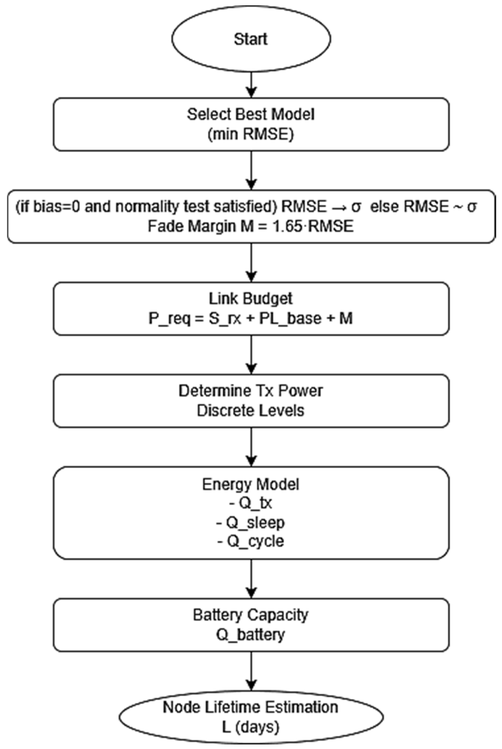
The proposed framework pipeline for node lifetime estimation is shown in Figure 2.

Algorithm 1 summarizes the complete workflow and serves as the sole procedural representation of the proposed framework.

Algorithm 1: System-Level Workflow

Input:

Dataset D = {distance d, frequency f, measured path loss PLmeas}

Step 1: Input dataset

x = [d, f],   y = PLmeas

Step 2: Model training and prediction

For each model m ∈ {Propagation model, ML, DL}:

Predict:

PLpred = f_m(x)

Compute:

RMSE_m = √(1/N Σ (PLpred − PLmeas)2)

m* = argmin(RMSEm)

Step 3: Residual computation

ε = PLmeas − f_{m*}(x)

Step 4: Statistical validation (interpretation metrics)

Compute:

p_bias (two-sided t-test for zero-mean residuals),

p_normality (Shapiro–Wilk test for Gaussianity)

Step 5: Dispersion representation

σest ← RMSEm* (empirical dispersion proxy under validated statistical assumptions)

Step 6: Reliability margin

M = 1.65 · σest

Step 7: Link budget

Preq = Srx + PLbase + M

Step 8: Transmission power mapping

Ptx = min{Pk ∈ P|Pk ≥ Preq}

Step 9: Energy consumption

Qcycle = f(Ptx)

Step 10: Node lifetime

L = (Qbattery/Qcycle) · T_interval

Output:

m*, RMSEm*, Ptx, Qcycle, L

4. Results

Learning-based models consistently demonstrate improved predictive performance compared to classical models. This is consistent with recent wireless propagation prediction studies using machine learning and ensemble methods [8,10,13,17,40]. Differences among learning-based models, particularly CNNs versus ensemble methods, require further interpretation in relation to feature space constraints and dataset characteristics.

4.1. Comparative Evaluation of Path Loss Prediction Models

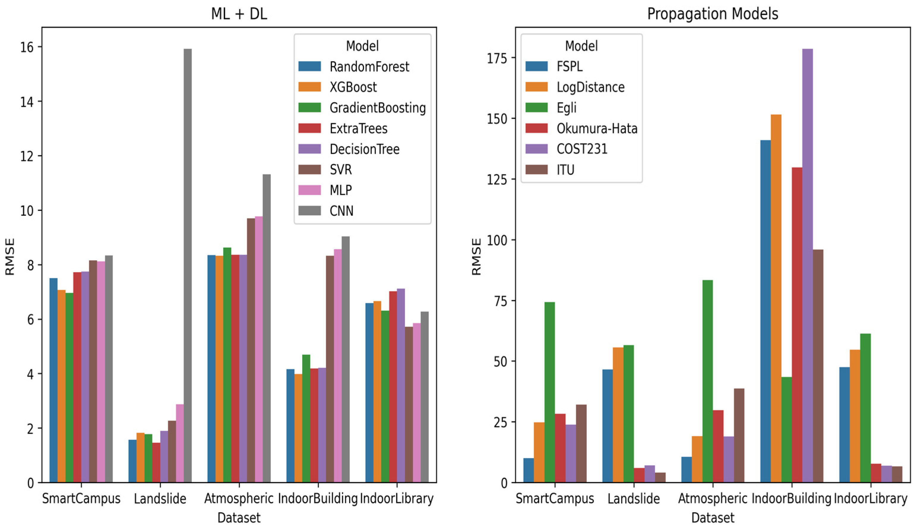
The proposed deployment-grade configurable framework is evaluated across five heterogeneous datasets representing realistic WSN–IoT deployment scenarios: outdoor environments (Smart Campus, Landslide), indoor cluttered environments (Indoor Building, Indoor Library), and high-frequency atmospheric propagation conditions. A uniform evaluation protocol was applied to all datasets, employing a 5-fold cross-validation protocol with shuffling and fixed random seed (random_state = 42), and assessing generalization performance on held-out folds, using RMSE, MAE, and R². Comparative benchmarking across heterogeneous indoor environments confirms that ensemble and deep learning models outperform classical regression-based propagation models, particularly under complex multipath and cluttered conditions [17]. The same test sets and evaluation metrics described in Section 3.2 were used consistently for all results reported in Figure 3 and Figure 4.

Table 6. Mean RMSE ± standard deviation across the 5-fold cross-validation procedure.

Prediction Method	Smart Campus	Landslide	Atmospheric	Indoor Building	Indoor Library
FSPL	10.042 ± 0.329	46.543 ± 0.428	10.503 ± 0.222	140.948 ± 0.309	47.459 ± 0.854
LogDistance	24.753 ± 0.234	55.647 ± 1.071	19.120 ± 0.350	151.552 ± 0.309	54.610 ± 0.762
Egli	74.233 ± 0.347	56.559 ± 2.709	83.359 ± 0.280	43.488 ± 0.471	61.235 ± 0.731
Okumura–Hata	28.226 ± 0.325	5.925 ± 1.981	29.803 ± 0.238	129.662 ± 0.386	7.733 ± 0.973
COST-231	23.843 ± 0.337	7.073 ± 0.586	18.918 ± 0.224	178.517 ± 0.382	6.923 ± 0.647
ITU	32.037 ± 0.230	4.072 ± 1.247	38.753 ± 0.260	95.844 ± 0.335	6.600 ± 0.860
RandomForest	7.498 ± 0.310	1.575 ± 0.240	8.351 ± 0.085	4.158 ± 0.169	6.586 ± 0.396
XGBoost	7.073 ± 0.250	1.826 ± 0.374	8.323 ± 0.098	3.983 ± 0.136	6.660 ± 0.476
GradientBoosting	6.956 ± 0.291	1.772 ± 0.355	8.623 ± 0.083	4.688 ± 0.056	6.304 ± 0.351
ExtraTrees	7.718 ± 0.315	1.461 ± 0.268	8.358 ± 0.079	4.184 ± 0.174	7.014 ± 0.454
DecisionTree	7.745 ± 0.335	1.890 ± 0.332	8.355 ± 0.095	4.215 ± 0.195	7.116 ± 0.543
SVR	8.156 ± 0.453	2.270 ± 1.176	9.699 ± 0.112	8.327 ± 0.299	5.714 ± 0.392
MLP	8.121 ± 0.332	2.868 ± 1.572	9.767 ± 0.186	8.563 ± 0.219	5.853 ± 0.309
CNN	8.331 ± 0.337	15.918 ± 1.638	11.317 ± 0.151	9.031 ± 0.176	6.275 ± 0.403

presents a comprehensive RMSE comparison across all evaluated analytical propagation models, machine learning (ML), and deep learning (DL) approaches. Classical empirical and semi-empirical models—such as FSPL, Log-Distance, Egli, Okumura–Hata, COST-231, and ITU—consistently exhibit substantially higher prediction errors across all deployment scenarios. This behavior reflects their reliance on simplified assumptions regarding propagation geometry, terrain homogeneity, and line-of-sight conditions, which limits their ability to adapt to heterogeneous and dynamically varying environments [1,2].

Across all evaluated models and datasets, the 5-fold cross-validation procedure not only provides mean performance estimates but also reveals consistent patterns in model stability across heterogeneous propagation environments. In particular, ensemble-based methods consistently exhibit lower RMSE variability across folds, indicating stable generalization behavior under different training–validation splits. XGBoost achieves RMSE_std values of 0.25 dB (Smart Campus), 0.09 dB (Atmospheric), and 0.13 dB (Indoor Building), while Gradient Boosting and other ensemble models show similarly consistent patterns across datasets. In contrast, CNN and SVR present higher variability, especially in the Landslide scenario, where CNN reaches RMSE_std = 1.64 dB and SVR = 1.18 dB, reflecting increased sensitivity to data partitioning under heterogeneous conditions. Overall, these results complement the mean RMSE analysis in Table 6 and confirm that ensemble methods provide a more favorable bias–variance trade-off across all evaluated propagation environments.

In contrast, learning-based models achieve significantly lower RMSE and MAE values, accompanied by systematically higher R² scores. The performance gap is particularly pronounced in indoor and terrain-affected outdoor environments, where multipath propagation, shadowing, and non-line-of-sight effects dominate signal attenuation. These results confirm the superior capability of data-driven approaches to approximate complex and nonlinear propagation behavior that cannot be adequately captured by closed-form analytical models [8,10]. The consistent trends observed across all datasets highlight the robustness of learning-based predictors under realistic deployment conditions where classical analytical assumptions no longer hold.

4.2. Best-Performing Models Across Deployment Scenarios

For each dataset, the best-performing model was identified based on minimum RMSE. The resulting best models and their corresponding performance metrics are summarized in

Table 7. Best-Performing Learning-Based model per Dataset (based on minimum RMSE).

Dataset	Best Model	MAE (dB)	RMSE (dB)	R2
Landslide	ExtraTrees	0.940	1.461	0.933
Indoor Building	XGBoost	2.767	3.983	0.937
Indoor Library	SVR	4.447	5.714	0.470
Smart Campus	Gradient Boosting	5.162	6.956	0.416
Atmospheric	XGBoost	6.636	8.323	0.720

, while comparative trends are illustrated in Figure 3. Ensemble-based ML methods—including Random Forest, Gradient Boosting, and XGBoost—consistently rank among the most accurate predictors across heterogeneous environments. This observation is fully consistent with prior studies, which demonstrated that ensemble learning methods such as Random Forest and XGBoost achieve the lowest RMSE and superior generalization performance in wireless path loss prediction tasks when evaluated using cross-validation protocols [40].

The lightweight CNN does not consistently outperform ensemble-based methods. This is mainly due to the very limited input feature space (distance and frequency), which does not provide the spatial or structured information required by convolutional architectures. As a result, the CNN behaves similarly to a generic nonlinear regressor, while ensemble models are more suitable for low-dimensional tabular data and achieve better bias–variance trade-offs. The observed behavior is therefore a consequence of feature representation rather than an inherent limitation of CNNs. From a computational perspective, the evaluated models exhibit different training and inference costs. Ensemble-based methods (e.g., Random Forest, XGBoost) provide a favorable trade-off between predictive accuracy and computational efficiency, with moderate training requirements and fast inference. In contrast, the CNN model involves higher training complexity due to iterative optimization and multiple training epochs, although inference remains relatively lightweight once the model is trained.

Given the deployment-oriented scope of the proposed framework, where model training is performed offline and predictions are used for system-level planning and design, the increased training cost of CNN models does not affect practical operation. Therefore, model selection is primarily driven by prediction accuracy and robustness rather than runtime constraints.

The observed differences in model performance across datasets can be directly attributed to the interaction between environmental propagation complexity and the inductive biases of each learning approach. In structured and moderately noisy environments (e.g., Landslide and Indoor Building), ensemble methods outperform other models due to their ability to partition the feature space effectively and capture localized nonlinearities without requiring explicit functional smoothness assumptions. In contrast, environments characterized by high variability and unobserved influencing factors (e.g., Smart Campus and Indoor Library) introduce stochasticity that reduces the effectiveness of purely deterministic regression boundaries, leading to lower R² values across all models despite relatively stable RMSE behavior. The CNN model does not consistently outperform tree-based ensembles because the input representation is strictly tabular (distance and frequency only), lacking spatial or grid-like structure that convolutional filters are designed to exploit. Similarly, SVR performs competitively in smoother propagation regimes but becomes less effective under highly heterogeneous conditions due to limited flexibility in partitioning complex, non-stationary error surfaces. Overall, these results indicate that model performance is primarily governed by the match between environmental complexity and model inductive bias rather than model capacity alone, with ensemble methods providing the most balanced performance across all evaluated propagation scenarios.

The strong performance of ensemble methods is attributed to their ability to aggregate multiple weak learners, thereby effectively balancing bias and variance while maintaining robustness to noise and dataset heterogeneity [21,22]. This advantage is especially evident in indoor and terrain-affected scenarios, where classical propagation models fail to capture site-specific attenuation mechanisms.

Lower R² values observed in the Indoor Library and Smart Campus datasets are not indicative of poor model behavior, but rather reflect the inherently high variability of these environments and the intentionally restricted feature space, which includes only distance and frequency. In such scenarios, substantial variance in measured path loss arises from unmodeled factors—such as dynamic human presence, furniture layout, building materials, antenna orientation, and local obstructions—placing an upper bound on achievable R² values. Importantly, despite reduced R², these models still achieve substantial reductions in absolute error (RMSE and MAE), which is the primary determinant of practical link budget accuracy.

The models reported in Table 4 correspond exclusively to the best-performing learning-based predictor for each dataset, selected strictly based on minimum RMSE on the test set, in accordance with the evaluation protocol defined in Section 4.2.

4.3. Measured vs. Predicted Path Loss Comparison and Implications for WSN–IoT Deployments

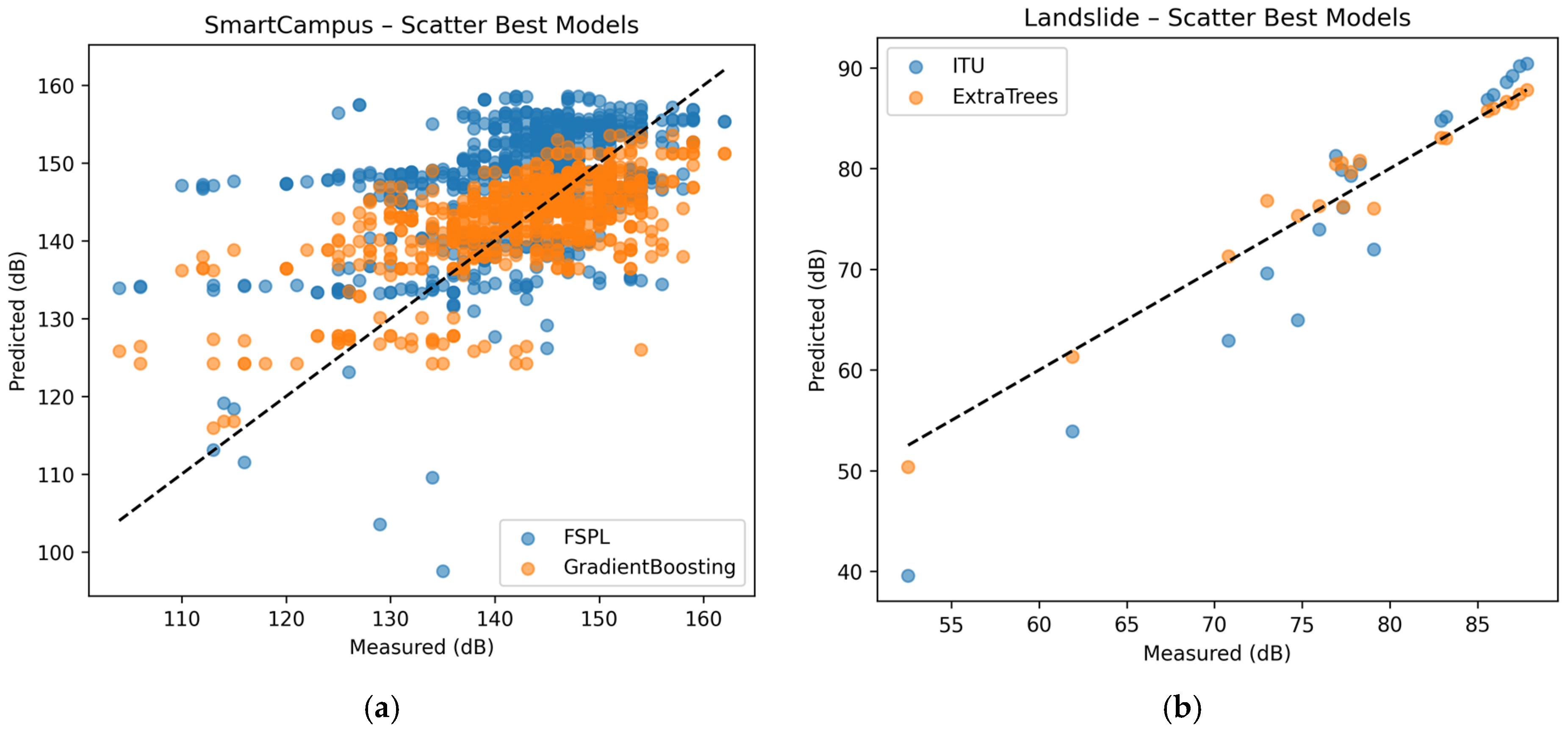
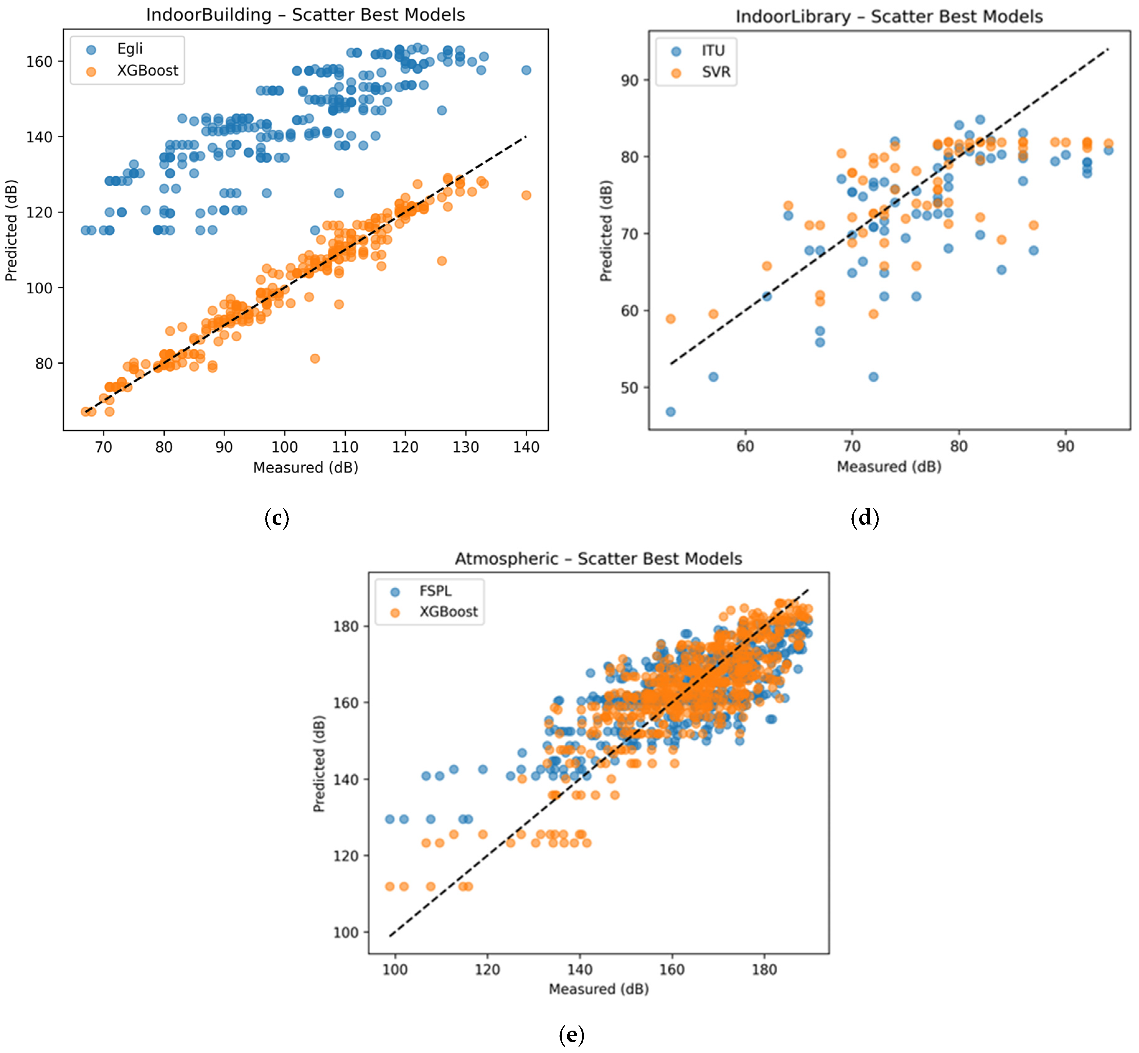
Measured and predicted path loss values are evaluated using the test set generated by a single independently trained model per dataset. The analysis relies on scatter plots of measured versus predicted values (Figure 4), which directly capture prediction accuracy, dispersion, and bias across the examined propagation scenarios. Prediction outputs are obtained from the final trained model, avoiding aggregation across cross-validation folds in order to preserve consistent error structure.

The scatter plots reveal distinct differences between classical propagation models and learning-based approaches. Classical models exhibit broader and often asymmetric dispersion around the ideal diagonal, with noticeable deviations at higher path loss values. These patterns indicate both increased prediction variance and systematic bias, reflecting the limited ability of analytical formulations to represent complex propagation effects under varying environmental conditions.

In contrast, learning-based models produce more compact and symmetric point distributions, closely aligned with the diagonal across the full range of values. This behavior indicates reduced variance and improved consistency, as well as a better balance between underestimation and overestimation errors. The tighter clustering is observed across all datasets, including those characterized by increased variability, demonstrating more stable generalization performance.

Differences in scatter structure are also evident across datasets. In scenarios with higher variability (lower R²), the dispersion increases for all models; however, learning-based approaches maintain more coherent distributions with fewer extreme deviations. The remaining spread is not associated with instability but reflects the stochastic nature of the propagation environment. This is further supported by the consistency between scatter patterns and the corresponding RMSE and MAE values reported in Section 4.2.

A direct comparison between the best-performing models confirms that machine learning predictors consistently achieve closer agreement with measured values, exhibiting reduced spread and minimal bias relative to classical models. In contrast, classical approaches show increasing dispersion and skewness as environmental complexity grows, particularly in high attenuation regions.

Overall, the scatter-based analysis demonstrates that learning-based models provide more accurate and stable predictions across diverse conditions, with error characteristics that remain consistent with the reported quantitative metrics. The observed dispersion patterns are therefore attributed to environmental variability rather than model-related deficiencies. CNN predictions show slightly higher dispersion compared to ensemble methods, consistent with the limitations imposed by the constrained feature space.

4.4. Statistical Significance and Residual Normality

Following the best model selection and in accordance with the statistical framework defined in Section 3.5.1, a structured residual analysis is performed to assess bias, normality, and the validity of reliability-aware interpretations. To ensure clarity in the interpretation of the reported error metrics, it is important to distinguish between the RMSE values presented in Table 7 and those reported in

Table 8. Structured statistical analysis of the residuals.

Dataset	Two-Sided p-Value	Shapiro p-Value	Normality	RMSE (dB)	σ (dB)
Landslide	0.253	0.093	True	1.8	1.78
Indoor Building	0.513	4.104 × 10−14	False	3.77	3.77
Indoor Library	0.076	0.585	True	6.23	6.14
Smart Campus	0.483	1.126 × 10−7	False	7.06	7.06
Atmospheric	0.486	0.630	True	8.15	8.15

. The RMSE values in Table 7 correspond to cross-validation performance metrics used for model selection, as described in Section 4.2. In contrast, the RMSE values in Table 8 are computed from the aggregated residual distribution of the selected best-performing model and are used for statistical analysis, including bias testing and variability estimation. Consequently, minor discrepancies between the two sets of RMSE values may arise due to differences in data partitioning, aggregation, and evaluation procedures.

The results indicate that, for all datasets, the residuals are statistically unbiased, as confirmed by the two-sided hypothesis test (p-value > 0.05), supporting the assumption of zero-mean error. Regarding normality, the Shapiro–Wilk test suggests that residuals follow an approximately Gaussian distribution in the Landslide, Indoor Library, and Atmospheric datasets, while deviations from normality are observed in the Indoor Building and Smart Campus datasets. Despite these deviations, the RMSE values remain numerically consistent with the estimated standard deviation (σ), confirming that RMSE serves as a reliable measure of dispersion across all scenarios. Under conditions of approximate normality and zero bias, this supports the interpretation of RMSE as an estimator of shadowing variability, in accordance with the framework defined in Section 3.5.1. In cases where normality is not strictly satisfied, RMSE should be interpreted as an effective empirical dispersion metric rather than a strict estimator of σ.

4.5. Energy-Aware Performance

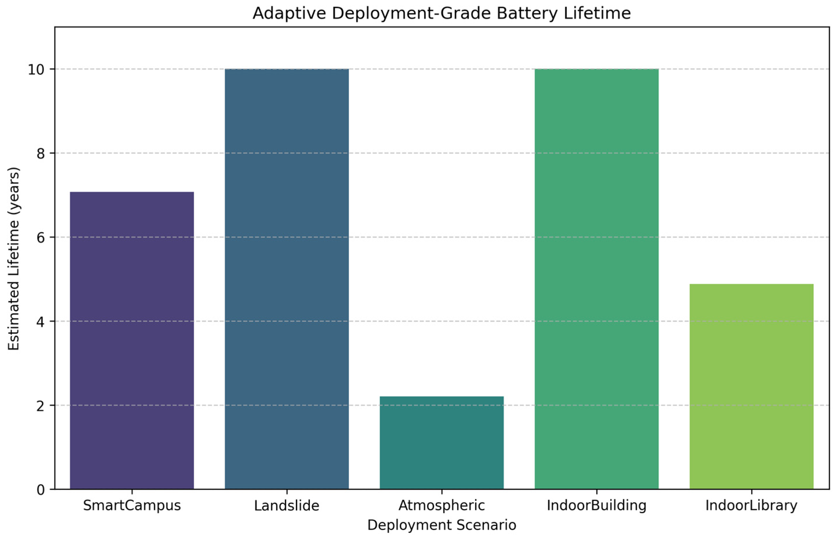
The improvements in prediction accuracy achieved by learning-based models have direct implications for wireless communication system design. More accurate path loss estimation enables refined link budgeting and reduced conservative fade margins. Beyond conventional accuracy metrics, the proposed framework incorporates a deployment-grade energy-aware analysis that explicitly links prediction error to transmission power requirements and node lifetime.

Table 9. Energy-aware deployment-grade performance using best-performance models.

Dataset	Best Model	RMSE (dB)	Pl_Base (dB)	Tx Power (dBm)	Estimated Lifetime (Years)
Smart Campus	Gradient Boosting	6.96	145.0	20.0	7.07
Landslide	Extra Trees	1.46	80.7	0.0	10.0
Atmospheric	XGBoost	8.32	164.9	20.0	2.21
Indoor Building	XGBoost	3.98	103.0	0.0	10.0
Indoor Library	SVR	5.71	77.0	0.0	4.88

summarizes the estimated operational lifetime for each deployment scenario using the best-performing prediction model, while Figure 5 provides a comparative visualization.

The results present a deployment-grade energy-aware analysis that directly links the predictive accuracy of the models with energy performance in realistic IoT scenarios. For each dataset, the reference path loss (base path loss) is computed as the median (PL50), while prediction uncertainty is incorporated through a fade margin equal to 1.65·RMSE, leading to the estimation of the required transmission power and, ultimately, the battery lifetime. The results reveal significant variations across scenarios: in SmartCampus, Gradient Boosting (RMSE = 6.96 dB, base PL = 145 dB) requires a transmission power of 20 dBm and achieves an estimated lifetime of 7.07 years, whereas in the Atmospheric scenario, despite the use of XGBoost, the high channel loss (164.9 dB) and RMSE = 8.32 dB also lead to 20 dBm transmission power but a substantially reduced lifetime of only 2.21 years. In contrast, in environments with lower path loss and higher prediction accuracy, such as Landslide (Extra Trees, RMSE = 1.46 dB, base PL = 80.7 dB) and Indoor-Building (XGBoost, RMSE = 3.98 dB, base PL = 103 dB), the required transmission power is limited to 0 dBm, enabling the maximum lifetime of up to 10 years.

The Indoor Library scenario (SVR, RMSE = 5.71 dB, base PL = 77 dB) requires 0 dBm transmission power and achieves a lifetime of 4.88 years, highlighting the combined impact of prediction accuracy and propagation conditions. The corresponding bar plot illustrates comparatively the estimated lifetime per scenario, clearly showing the energy burden in demanding environments and the benefits of more accurate models. The main contribution of this study lies in introducing a fully adaptive, data-driven framework that translates prediction error (RMSE) into practical design metrics, such as node lifetime. From a practical perspective, this approach provides network designers with a direct and quantitative decision-support tool, enabling informed identification of propagation models and operating parameters to optimize energy efficiency and maximize the lifetime of IoT nodes under real deployment conditions.

The experimental evaluation, in alignment with the deployment-oriented results, confirms that ML approaches generally outperform classical propagation models in the evaluated datasets in realistic, cluttered, and heterogeneous wireless environments, particularly when prediction accuracy is directly translated into energy performance metrics. While analytical models retain physical interpretability, their fixed formulations limit their ability to adapt to complex propagation phenomena such as multipath fading, shadowing, and non-line-of-sight (NLoS) conditions—limitations that become critical in dense WSN and IoT deployments. In contrast, learning-based models capture these effects implicitly, leading not only to more accurate path loss predictions but also to more reliable estimation of fade margins (1.65 × RMSE), transmission power, and battery lifetime, as demonstrated across diverse scenarios (e.g., high-loss Atmospheric vs. low-loss Landslide and Indoor-Building environments).

Among the evaluated approaches, ensemble learning methods consistently achieve the lowest prediction errors, translating into reduced uncertainty, lower required transmission power (down to 0 dBm in favorable conditions), and significantly extended node lifetime (up to 10 years), while necessitate the highest available transmission power level defined by the corresponding hardware profile (e.g., 20 dBm in the evaluated scenarios) and result in substantially reduced lifetime. Deep learning models such as CNNs depend strongly on structured and information-rich inputs. Ιn this study, the limited feature space restricts their advantage compared to ensemble methods. From a system-level perspective, absolute error metrics such as RMSE and MAE prove more meaningful than R², as they directly drive practical design parameters including link budgeting, fade margin allocation, and transmission power estimation within discrete hardware constraints. Beyond accuracy, the results indicate that reductions in RMSE are associated with lower fade margins and improved energy efficiency.

The proposed framework therefore bridges the gap between predictive modeling and system design by linking error metrics with energy provisioning parameters, offering actionable, quantitative decision support for network planners. Despite the use of minimal input features (distance and frequency) for fair comparison, the findings suggest that incorporating richer environmental descriptors and exploring hybrid or adaptive ML schemes could further enhance performance. Overall, the study demonstrates that ML-based path loss modeling is not only more accurate but also fundamentally enables energy-efficient, scalable, and reliable operation in dense IoT and WSN deployments.

Results are derived from dataset-isolated evaluation and should be interpreted within each propagation domain. Consistent trends across datasets indicate robustness, while absolute differences may reflect underlying distributional variability rather than purely model-related effects.

5. Conclusions and Future Work

This work introduced a deployment-oriented and energy-aware framework for evaluating path loss prediction methods in wireless sensor network (WSN) and IoT systems, explicitly linking propagation modeling with system-level design and operational energy performance. By standardizing datasets, feature sets, and evaluation metrics, the framework enables fair and consistent comparison between classical propagation models and learning-based approaches, while translating prediction accuracy into practical design parameters such as fade margin (1.65 × RMSE), required transmission power, and battery lifetime.

The results indicate that data-driven models—particularly ensemble learning methods—demonstrate superior performance in most evaluated scenarios, both in terms of prediction accuracy and energy efficiency. Lower RMSE values reduce uncertainty, leading to smaller fade margins and lower transmission power (e.g., 0 dBm in favorable scenarios such as Landslide and Indoor Building), thereby maximizing node lifetime (up to 10 years). In contrast, higher prediction errors in challenging environments (e.g., Atmospheric) require the highest available transmission power defined by the hardware profile (e.g., 20 dBm), resulting in significantly reduced lifetime. Even with a limited feature set (distance and frequency), learning-based models effectively capture complex attenuation behaviors that static models cannot represent, enabling more reliable link budget estimation and supporting network planning and deployment decisions.

By embedding prediction accuracy within a deployment-grade link budget analysis, the framework provides a quantitative view of how modeling errors propagate to system-level metrics, including reliability margins, energy consumption, and network lifetime. This linkage enables a shift from purely statistical evaluation to a decision-oriented perspective, where improvements in RMSE are associated with enhanced energy efficiency, reduced over-provisioning, and more effective transmission power estimation in large-scale, battery-constrained IoT deployments.

The relatively lower performance of the CNN is primarily attributed to the constrained feature space and dataset characteristics, including a limited number of samples in certain datasets (e.g., 100 samples in the Landslide dataset), rather than indicating inherent limitations of deep learning approaches. This suggests that the CNN behavior is conditioned by data availability and input representation rather than model capacity.

Overall, the framework establishes a unified workflow that bridges predictive modeling with network design, supporting informed decisions from early-stage planning to topology optimization and long-term energy management. Although the study adopts a minimal and controlled feature space to ensure fair cross-dataset comparison, the results highlight the potential benefits of incorporating richer environmental descriptors and advancing toward hybrid, physics-informed, and adaptive machine learning models. Future work may additionally investigate probabilistic and uncertainty-aware learning approaches, including Bayesian and quantile-based formulations, to further refine uncertainty propagation and reliability-aware communication system design. Ultimately, the proposed methodology demonstrates that accurate path loss modeling extends beyond predictive performance, serving as a key enabler for scalable, energy-efficient, and reliable WSN–IoT systems under real-world deployment conditions.

References

1. Rappaport, T.S. Wireless Communications: Principles and Practice, 2nd ed.; Prentice Hall: Upper Saddle River, NJ, USA, 2002; pp. 139–185. [Google Scholar]
2. Goldsmith, A. Wireless Communications; Cambridge University Press: Cambridge, UK, 2005; pp. 27–88. [Google Scholar]
3. Olasupo, T.O.; Otero, C.E.; Otero, L.D.; Olasupo, K.O. Path Loss Models for Low-Power, Low-Data-Rate Sensor Nodes for Smart Car Parking Systems. IEEE Trans. Intell. Transp. Syst. 2018, 19, 1774–1783. [Google Scholar] [CrossRef]
4. Akyildiz, I.F.; Su, W.; Sankarasubramaniam, Y.; Cayirci, E. Wireless Sensor Networks: A Survey. Comput. Netw. 2002, 38, 393–422. [Google Scholar] [CrossRef]
5. Raghunathan, V.; Schurgers, C.; Park, S.; Srivastava, M.B. Energy-Aware Wireless Microsensor Networks. IEEE Signal Process. Mag. 2002, 19, 40–50. [Google Scholar] [CrossRef]
6. Anastasi, G.; Conti, M.; Di Francesco, M.; Passarella, A. Energy Conservation in Wireless Sensor Networks: A Survey. Ad Hoc Netw. 2009, 7, 537–568. [Google Scholar] [CrossRef]
7. Sun, S.; Rappaport, T.S.; Rangan, S.; Thomas, T.A.; Ghosh, A.; Kovács, I.Z.; Rodriguez, I.; Koymen, O.; Partyka, A.; Jarvelainen, J. Propagation path loss models for 5G urban micro- and macro-cellular scenarios. In Proceedings of the IEEE 83rd Vehicular Technology Conference (VTC-Fall), Montreal, QC, Canada, 18–21 September 2016. [Google Scholar]
8. Zhang, Y.; Wen, J.; Yang, G.; He, Z.; Wang, J. Path Loss Prediction Based on Machine Learning: Principle, Method, and Data Expansion. Appl. Sci. 2019, 9, 1908. [Google Scholar] [CrossRef]
9. He, R.; Ai, B.; Wang, G.; Zhong, Z.; Molisch, A.F. Machine Learning for Wireless Channel Modeling: An Overview. IEEE Commun. Mag. 2019, 57, 91–97. [Google Scholar] [CrossRef]
10. Jiang, W.; Schotten, H.D. Machine Learning for Wireless Communications in the Internet of Things: A Comprehensive Survey. IEEE Commun. Surv. Tutor. 2020, 22, 1780–1810. [Google Scholar] [CrossRef]
11. Kwon, B.; Son, H. Accurate path loss prediction using a neural network ensemble method. Sensors 2024, 24, 304. [Google Scholar] [CrossRef] [PubMed]
12. Iliev, I.; Velchev, Y.; Petkov, P.Z.; Bonev, B.; Iliev, G.; Nachev, I. A Machine Learning Approach for Path Loss Prediction Using Combination of Regression and Classification Models. Sensors 2024, 24, 5855. [Google Scholar] [CrossRef] [PubMed]
13. Idogho, J.; George, G. Path Loss Prediction Based on Machine Learning Techniques: Support Vector Machine, Artificial Neural Network, and Multilinear Regression Model. Open J. Phys. Sci. OJPS 2022, 3, 1–22. [Google Scholar] [CrossRef]
14. Halifa, A.; Ampomah, E.A.; Gyasi, K.O.; Agyekum, K.O.-B.O.; Kwakye, K.S.O.; Shukla, P.K. A Comparative Analysis of Machine Learning Ensemble Methods for Accurate Path Loss Prediction. J. Electr. Syst. 2024, 20, 8467. [Google Scholar] [CrossRef]
15. Kendall, A.; Gal, Y. What Uncertainties Do We Need in Bayesian Deep Learning for Computer Vision? In Advances in Neural Information Processing Systems 30 (NeurIPS 2017); Guyon, I., von Luxburg, U., Bengio, S., Wallach, H., Eds.; Curran Associates, Inc.: Red Hook, NY, USA, 2017; pp. 5574–5584. [Google Scholar]
16. Lakshminarayanan, B.; Pritzel, A.; Blundell, C. Simple and Scalable Predictive Uncertainty Estimation Using Deep Ensembles. In Advances in Neural Information Processing Systems 30 (NeurIPS 2017); Guyon, I., von Luxburg, U., Bengio, S., Wallach, H., Eds.; Curran Associates, Inc.: Red Hook, NY, USA, 2017; pp. 6402–6413. [Google Scholar]
17. Elmezughi, M.K.; Salih, O.; Afullo, T.J.; Duffy, K.J. Comparative Analysis of Major Machine-Learning-Based Path Loss Models for Enclosed Indoor Channels. Sensors 2022, 22, 4967. [Google Scholar] [CrossRef]
18. Moraitis, N.; Psychogios, K.; Panagopoulos, A.D. A Survey of Path Loss Prediction and Channel Models for Unmanned Aerial Systems for System-Level Simulations. Sensors 2023, 23, 4775. [Google Scholar] [CrossRef]
19. Stone, M. Cross-validatory Choice and Assessment of Statistical Predictions. J. R. Stat. Soc. Ser. B 1974, 36, 111–147. [Google Scholar] [CrossRef]
20. Kuhn, M.; Johnson, K. Applied Predictive Modeling; Springer: New York, NY, USA, 2013. [Google Scholar]
21. Breiman, L. Random forests. Mach. Learn. 2001, 45, 5–32. [Google Scholar] [CrossRef]
22. Friedman, J. Greedy Function Approximation: A Gradient Boosting Machine. Ann. Stat. 2001, 29, 1189–1232. [Google Scholar] [CrossRef]
23. Chen, T.; Guestrin, C. XGBoost: A Scalable Tree Boosting System. In Proceedings of the 22nd ACM SIGKDD International Conference on Knowledge Discovery and Data Mining, San Francisco, CA, USA, 13–17 August 2016; pp. 785–794. [Google Scholar] [CrossRef]
24. Geurts, P.; Ernst, D.; Wehenkel, L. Extremely Randomized Trees. Mach. Learn. 2006, 63, 3–42. [Google Scholar] [CrossRef]
25. Yong, T.; Lee, C.; Kim, S.; Kim, J. Battery Life Prediction for Ensuring Robust Operation of IoT Devices in Remote Metering. Appl. Sci. 2025, 15, 2968. [Google Scholar] [CrossRef]
26. Heinzelman, W.R.; Chandrakasan, A.; Balakrishnan, H. Energy-Efficient Communication Protocol for Wireless Microsensor Networks. In Proceedings of the 33rd Annual Hawaii International Conference on System Sciences, Maui, HI, USA, 7 January 2000. [Google Scholar] [CrossRef]
27. Yick, J.; Mukherjee, B.; Ghosal, D. Wireless Sensor Network Survey. Comput. Netw. 2008, 52, 2292–2330. [Google Scholar] [CrossRef]
28. Alobaidy, H.A.H.; Singh, M.J.; Behjati, M.; Nordin, R.; Abdullah, N.F. Wireless Transmissions, Propagation and Channel Modelling for IoT Technologies: Applications and Challenges. IEEE Access 2022, 10, 24095–24131. [Google Scholar] [CrossRef]
29. Aldossari, S.A. Predicting Path Loss of an Indoor Environment Using Artificial Intelligence in the 28-GHz Band. Electronics 2023, 12, 497. [Google Scholar] [CrossRef]
30. Ndzi, D.L.; Kamarudin, L.M.; Zakaria, A.; Ndzi, E.; Jafaar, M.H.; Kamarudin, K. A Comparative Analysis of Path Loss Models for Wireless Sensor Networks Using Machine Learning Techniques. IEEE Access 2018, 6, 31645–31654. [Google Scholar] [CrossRef]
31. Drucker, H.; Burges, C.J.C.; Kaufman, L.; Smola, A.; Vapnik, V. Support Vector Regression Machines. In Advances in Neural Information Processing Systems (NeurIPS 1996); Mozer, M.C., Jordan, M.I., Petsche, T., Eds.; MIT Press: Cambridge, MA, USA, 1997; pp. 155–161. [Google Scholar]
32. Wu, X.; Wang, H.; Zhang, Y.; Zou, B.; Hong, H. A Tutorial-Generating Method for Autonomous Online Learning. IEEE Trans. Learn. Technol. 2024, 17, 1558–1567. [Google Scholar] [CrossRef]
33. Zhu, R.; Li, W.; Boukerche, A.; Yang, Q. Energy-Aware DRL-Based Dual-Perception Fountain Codes for Resource-Constrained Underwater Acoustic Sensor Networks. IEEE Trans. Sustain. Comput. 2026, 11, 111–122. [Google Scholar] [CrossRef]
34. IEEE Standard 802.15.4; IEEE Standard for Low-Rate Wireless Networks. IEEE: New York, NY, USA, 2020.
35. Ratul, R.H.; Zaman, S.M.M.; Chowdhury, H.A.; Sagor, M.Z.H.; Kawser, M.T.; Nishat, M.M. Atmospheric Influence on the Path Loss at High Frequencies for Deployment of 5G Cellular Communication Networks. In Proceedings of the 2023 14th International Conference on Computing Communication and Networking Technologies (ICCCNT), Delhi, India, 6–8 July 2023; Available online: https://ieeexplore.ieee.org/abstract/document/10307972 (accessed on 10 April 2026).
36. Popoola, S.I.; Atayero, A.A.; Arausi, O.D.; Matthews, V.O. Path Loss Dataset for Modeling Radio Wave Propagation in Smart Campus Environment. Data Brief 2018, 17, 1062–1073. [Google Scholar] [CrossRef]
37. El Chall, R.; Lahoud, S.; El Helou, M. LoRaWAN Measurement Campaigns in Lebanon Indoor Building Dataset. Zenodo. 2018. Available online: https://zenodo.org/records/1560654 (accessed on 26 February 2026).
38. Meneses Viveros, A.; Galván Tejada, G.M.; Perdomo Reyes, P. Path Loss Dataset from Field Measurements at 3.5 GHz for the Fifth Generation of Wireless Communications in Indoor Environments. Sci. Data 2026, 13, 521. Available online: https://www.nature.com/articles/s41597-026-06650-4 (accessed on 26 February 2026). [CrossRef]
39. Shutimarrungson, N.; Wuttidittachotti, P. Realistic Propagation Effects on Wireless Sensor Networks for Landslide Management. EURASIP J. Wirel. Commun. Netw. 2019, 2019, 94. [Google Scholar] [CrossRef]
40. Elmezughi, M.K.; Salih, O.; Afullo, T.J.; Duffy, K.J. Path Loss Modeling Based on Neural Networks and Ensemble Method for Future Wireless Networks. Heliyon 2023, 9, e19685. [Google Scholar] [CrossRef] [PubMed]
41. Breiman, L.; Friedman, J.; Olshen, R.; Stone, C.J. Classification and Regression Trees; Wadsworth & Brooks/Cole: Monterey, CA, USA, 1984. [Google Scholar]
42. Rumelhart, D.E.; Hinton, G.E.; Williams, R.J. Learning Representations by Back-Propagating Errors. Nature 1986, 323, 533–536. [Google Scholar] [CrossRef]
43. Papastergiou, G.; Xenakis, A.; Chaikalis, C.; Kosmanos, D.; Papastergiou, M.P. Enhancing IoT Connectivity in Suburban and Rural Terrains Through Optimized Propagation Models Using Convolutional Neural Networks. IoT 2025, 6, 41. [Google Scholar] [CrossRef]
44. Shapiro, S.S.; Wilk, M.B. An Analysis of Variance Test for Normality. Biometrika 1965, 52, 591–611. [Google Scholar] [CrossRef]
Figure 1. Communication model between two nodes [34].
Electronics 15 02350 g001
Figure 2. Statistically grounded transformation pipeline from prediction error to system-level metrics.
Electronics 15 02350 g002
Figure 3. RMSE comparison between learning-based and propagation models.
Electronics 15 02350 g003
Figure 4. Measured versus predicted path loss for the best-performing learning-based model across all deployment scenarios: (a) Smart Campus, (b) Landslide, (c) Indoor Building, (d) Indoor Library, and (e) Atmospheric. The multi-panel representation facilitates direct comparison of prediction agreement and dispersion across heterogeneous propagation environments. The dashed diagonal line represents the ideal agreement between measured and predicted path loss values.
Electronics 15 02350 g004aElectronics 15 02350 g004b
Figure 5. Comparison of estimated node lifetime across deployment scenarios using the best-performing prediction model for each dataset.
Electronics 15 02350 g005