Adaptive Control Strategy for a Single-Inverter Dual-PMSM System Under Load Disturbance

Abstract

To address the speed oscillation and stability degradation caused by load imbalance in a single−inverter dual−permanent magnet synchronous motor (PMSM) parallel system, this paper proposes an adaptive control strategy based on a sliding mode observer. The proposed method preserves the hardware simplicity of the single−inverter topology while improving control performance under load disturbances. First, a sliding mode observer is designed to estimate the load torque difference between the two motors in real time, thereby enabling dynamic perception of load variations. Then, an adaptive controller is introduced to switch the control mode according to the estimated load imbalance. When the load difference is small, master−slave vector control without fixed role distinction is adopted. When the load difference exceeds a predefined threshold, an improved finite−set model predictive torque control (FCS−MPTC) is activated. In the predictive control mode, unnecessary full−time predictive optimization is avoided and a d−axis current suppression term is incorporated into the cost function to improve current waveform quality. Simulation results show that the proposed strategy reduces speed overshoot during load transients and improves the three−phase current waveform compared with conventional predictive torque control. Therefore, the proposed method provides an effective control solution for single−inverter dual−motor drive systems under load disturbance.

1. Introduction

In industrial drive systems such as electric vehicles, wind power generation, gantry cranes, pump systems, and CNC machine tools, permanent magnet synchronous motors (PMSMs) have been widely used because of their high power density, high efficiency, and favorable dynamic performance [1,2,3,4,5]. 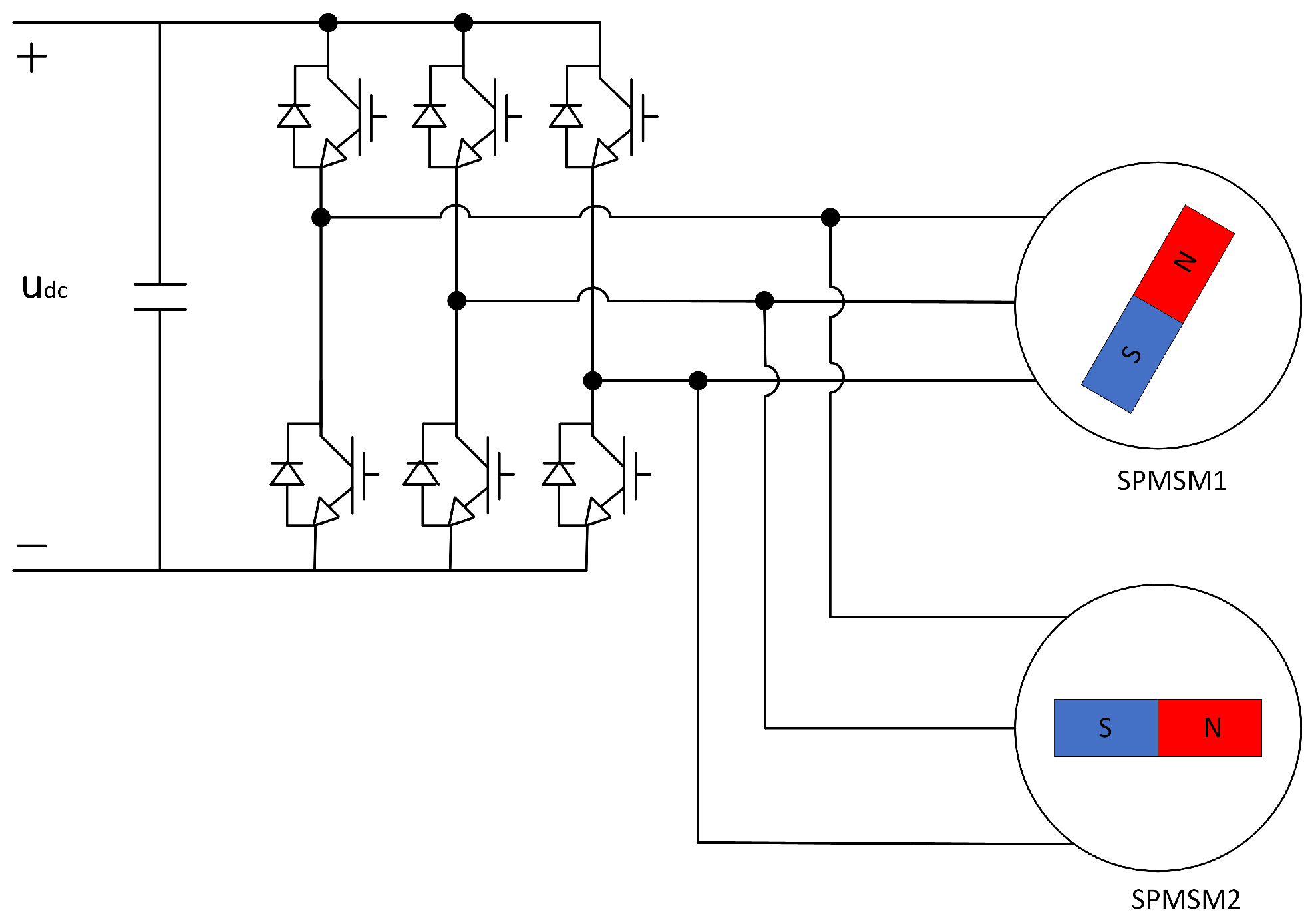With the increasing demand for compact and cost−effective multi−motor drive systems, conventional multi−inverter drive schemes may suffer from increased hardware cost, larger system volume, and more complex control implementation [6,7]. To reduce the number of power converters, the single−inverter dual−PMSM parallel topology has attracted increasing attention in recent years [8,9,10,11]. In this topology, two PMSMs share the same inverter output, which reduces the number of power switching devices and simplifies the hardware structure compared with dual−inverter configurations. However, the shared inverter also means that the two motors are driven by the same voltage vector, making their electrical and mechanical states strongly coupled. Therefore, although the single−inverter dual−PMSM topology is attractive for low−cost integrated drive systems, it also brings new challenges for speed synchronization and load−disturbance suppression.

In a single−inverter dual−PMSM system, the two motors are expected to maintain speed synchronization when operating under balanced load conditions. However, once the load torques of the two motors become unequal, the shared inverter output cannot independently compensate the two motors. The asymmetric load demand changes the rotor position difference and torque−angle relationship, which may further induce speed desynchronization, torque oscillation, and even transient instability. Therefore, load imbalance in this topology is not only an external disturbance, but also a key factor affecting the internal coupling state of the dual−motor system. To address this problem, various control strategies have been reported in the literature [12,13,14].

Master−slave control is one of the earliest and most commonly used strategies for single−inverter dual−PMSM systems [15]. In this method, one motor is selected as the master motor and regulated in closed loop, whereas the other motor operates as the slave motor under open−loop or indirectly constrained control [16]. Owing to its simple structure and low computational burden, master−slave control is suitable for balanced or mildly unbalanced operating conditions. However, its control performance strongly depends on the correct assignment of the master motor. When the load applied to the slave motor becomes larger than that of the master motor, the fixed maste−slave relationship may no longer reflect the actual load distribution, which can lead to speed oscillation, torque−angle deviation, or even transient instability. Active damping control can suppress part of the speed oscillation by adjusting the d−axis current [17]; nevertheless, its effectiveness may degrade when the motor parameters or rotational inertias are mismatched. More importantly, these methods still rely on an explicit master−slave distinction and do not provide a load imbalance−aware mechanism for allocating different control modes according to the real−time operating condition of the dual−motor system.

To overcome the limitation of fixed master−slave assignment, load−dependent master selection has been investigated [18]. In this type of method, the motor subjected to the higher load is selected as the master motor, so that the torque power angles of both motors can be maintained within the stable operating region. This strategy improves the stability of conventional fixed master−slave control under unequal load conditions. However, it still requires real−time load torque observation to identify the master motor, and the controller remains dependent on an explicit master−slave relationship. When the load distribution changes rapidly, frequent role switching between the two motors may introduce additional transient fluctuations and degrade the speed synchronization performance. Therefore, although load−dependent master−slave control improves the role assignment problem to some extent, it does not fundamentally provide a hybrid control allocation mechanism according to the degree of load imbalance.

Average model control has also been introduced to avoid the explicit master−slave distinction by using the average speed, position, and current of the two motors as feedback variables [19]. In some studies, weighted or optimized control variables are constructed according to the load condition of the two motors to improve synchronization and efficiency under unequal load conditions [20]. Compared with conventional master−slave control, average model control can reduce the dependence on a fixed master motor and maintain acceptable stability when the load difference is small. However, by treating the two motors as an equivalent controlled object, the asymmetric load information of each motor may be weakened or even masked by the averaged variables. As a result, the controller may not respond effectively when one motor is subjected to a sudden or significantly larger load disturbance. In addition, because the two motors are strongly coupled through the shared inverter output, the performance of average model control is sensitive to parameter mismatch and model uncertainty. Therefore, average model control does not provide an explicit load−imbalance perception mechanism or a control−mode allocation strategy for strongly unbalanced operating conditions.

Model predictive control (MPC) has also been investigated for single−inverter dual−motor systems [21,22,23,24]. Compared with PI−based vector control, MPC can handle multivariable control objectives and improve dynamic response by directly evaluating candidate voltage vectors. In finite−control−set model predictive control (FCS−MPC), the optimal voltage vector is usually selected by minimizing a cost function related to torque, flux, current, or speed tracking errors. However, conventional FCS−MPC still faces several practical limitations. First, all candidate voltage vectors are generally predicted and evaluated in each sampling period, which increases the online computational burden. Second, different control objectives in the cost function usually have different physical units and dynamic ranges, making the weighting-factor selection empirical and case-dependent. Third, because FCS-MPC directly selects discrete switching states without a fixed modulation pattern, the switching frequency is variable, which may deteriorate current waveform quality and introduce electromagnetic interference, mechanical vibration, acoustic noise, and additional switching losses [25].

To improve the practical applicability of MPC, recent adaptive MPC and hybrid predictive control methods have been developed by introducing weighting-factor elimination, weighting-factor adaptation, fast voltage-vector selection, low-complexity optimization, observer-based disturbance compensation, and model-free or hybrid predictive control structures [26,27,28,29,30]. These methods can reduce parameter-tuning effort, improve robustness, or decrease the online computational burden of predictive control. Nevertheless, most existing adaptive or hybrid MPC strategies mainly focus on improving the predictive controller itself, such as optimizing the cost function, reducing the candidate voltage-vector set, or compensating external disturbances. For single-inverter dual-PMSM systems, the two motors share the same inverter output, and load imbalance directly changes the coupled operating condition of the dual-motor system. Therefore, the key issue is not only how to improve the predictive controller, but also how to determine when predictive control should be activated according to the real-time load imbalance. Existing adaptive MPC or hybrid control frameworks have not sufficiently exploited the estimated load-torque difference as a physical decision variable for control-mode allocation between low-complexity vector control and predictive torque control.

In addition to predictive control, disturbance estimation and sliding-mode observer-based methods have also been widely investigated to improve the robustness of PMSM drives under parameter uncertainties and load disturbances. Sliding mode observers are attractive for motor-drive systems because of their simple structure, strong robustness against disturbances, and suitability for real-time implementation. For PMSM drives, SMO-based methods have been used to estimate load torque, rotor speed, rotor position, and lumped disturbances, thereby improving disturbance rejection and dynamic tracking performance. In recent years, advanced sliding-mode methods, such as adaptive sliding-mode observers, super-twisting sliding-mode observers, generalized super-twisting sliding-mode control, and observer-assisted robust control, have been developed to reduce chattering and improve estimation accuracy [31,32,33,34].

For example, Lin et al. [31] proposed an adaptive generalized super-twisting sliding-mode control method for PMSMs with a filtered high-gain observer, in which the observer was used to estimate lumped disturbances caused by parameter uncertainties and external load torque disturbances. Kang et al. [32] further developed an adaptive generalized super-twisting sliding mode control strategy for PMSM drives to improve finite-time convergence and robustness under disturbances. Event-triggered generalized super-twisting sliding-mode control has also been investigated for PMSM position tracking to reduce unnecessary control updates while maintaining robust tracking performance [33]. In addition, Shen et al. [34] combined event-triggered FCS-MPC with a sliding-mode observer for PMSM servo motion systems, where the SMO was used to identify load torque and enhance disturbance rejection while reducing redundant predictive control actions.

However, most existing SMO-based or super-twisting sliding-mode methods are mainly developed for single PMSM drives, where the estimated disturbance is generally used for speed regulation, position tracking, or disturbance compensation. In a single-inverter dual-PMSM system, the two motors share the same inverter output, and the key problem is not only disturbance estimation for a single motor, but also how to use the estimated load imbalance between the two motors to determine the appropriate control mode. Therefore, this paper further uses the estimated load-torque difference as a physical decision variable for adaptive mode allocation between vector control and predictive torque control.

Despite these efforts, a clear research gap still remains in the control of single-inverter dual-PMSM systems under load disturbance. Existing master–slave control methods mainly rely on fixed or load-dependent role assignment, and their transient performance may deteriorate when the load distribution changes abruptly. Average model-based methods reduce the dependence on explicit master–slave roles, but the use of averaged feedback variables may weaken the asymmetric load information between the two motors. Conventional FCS-MPC can improve dynamic response, but full-time predictive optimization increases the computational burden and may degrade current waveform quality due to variable switching frequency. Recent adaptive MPC and hybrid predictive control methods have improved weighting-factor design, voltage-vector selection, and disturbance compensation; however, they mainly focus on improving the predictive controller itself rather than exploiting the load imbalance as a decision variable for control-mode allocation. Therefore, the key unresolved issue is how to use the real-time load-torque difference as a physical indicator to distinguish balanced and strongly unbalanced operating conditions, and to adaptively allocate low-complexity vector control and predictive torque control in the strongly coupled single-inverter dual-PMSM system.

To address this research gap, this paper proposes a load imbalance-aware hybrid control strategy for a single-inverter dual-PMSM system. The novelty of the proposed method does not lie in the isolated use of an SMO or predictive control. Instead, the SMO-estimated load-torque difference is used as a physical indicator of the operating condition of the strongly coupled dual-motor system. Based on this indicator, the controller adaptively allocates the control mode according to the degree of load imbalance. When the estimated load-torque difference is small, a vector-control−based strategy is adopted to maintain speed synchronization with low computational cost and without relying on permanently fixed master−slave role assignment. When the estimated load−torque difference exceeds a predefined threshold, FCS−MPTC is activated to enhance disturbance rejection and dynamic synchronization performance under strongly unbalanced load conditions. In this way, the proposed strategy avoids unnecessary full−time predictive optimization under normal operating conditions while improving transient response under large load disturbances. To further clarify the differences between representative control frameworks and the proposed method,

Table 1. Critical comparison of representative control frameworks.

Control Framework	Main Advantage	Main Limitation	Difference from the Proposed Method
Conventional master−slave control	Simple structure and low computational burden	Sensitive to fixed or inappropriate master−slave role assignment under load variation	The proposed method avoids dependence on fixed master−slave role assignment under balanced or weakly unbalanced conditions
Average model−based control	Avoids explicit master−slave distinction	Averaged variables may mask asymmetric load information between the two motors	The proposed method uses the estimated load−torque difference rather than averaged feedback variables
Conventional FCS−MPC	Fast dynamic response and multivariable optimization capability	Full−time online optimization, empirical weighting−factor tuning, and variable switching frequency	The proposed method activates predictive torque control only under significant load imbalance
Recent adaptive/hybrid MPC	Improves weighting−factor design, voltage−vector selection, robustness, or computational efficiency	Mainly focuses on improving the predictive controller itself	The proposed method uses load imbalance as the decision variable for hybrid control−mode allocation
Proposed method	Load imbalance−aware control−mode allocation	Requires proper observer gain design and load−imbalance threshold selection	Specifically designed for strongly coupled single−inverter dual−PMSM systems under load imbalance

summarizes their main advantages, limitations, and distinctions.

The main contributions of this study are summarized as follows:

(1)

A load imbalance−aware hybrid control framework is proposed for the strongly coupled single−inverter dual−PMSM system. Unlike conventional master−slave control, average model−based control, or full−time predictive control, the proposed framework uses the real−time load−torque difference as an operating−condition indicator for adaptive control−mode allocation.

(2)

An SMO−based load−torque difference estimation method is integrated into the control−mode selection mechanism. The estimated load−torque difference is not only used for disturbance perception, but also serves as the decision variable for distinguishing balanced or weakly unbalanced operating conditions from strongly unbalanced operating conditions.

(3)

A conditional predictive torque control mechanism is developed to balance dynamic response and current waveform quality under load disturbance. Under balanced or weakly unbalanced load conditions, vector control is adopted to avoid unnecessary predictive optimization; under strongly unbalanced load conditions, FCS−MPTC with a $d-$axis current suppression term is activated to enhance disturbance rejection, speed synchronization, and current waveform quality.

2. Single−Inverter Dual−Permanent Magnet Synchronous Motor

2.1. Single−Inverter Dual−Permanent Magnet Synchronous Motor Model

Figure 1 shows the structure of the single−inverter dual surface−mounted PMSM system. Two surface−mounted PMSMs with identical parameters are connected in parallel to the three−phase output of a common inverter.

The stator voltage equation and the flux−linkage equation of each motor in the $dq$ reference frame are given as follows:

$$\left\{\begin{array}{cc}\hfill u_d& =R_s{i}_d+{\displaystyle \frac{d{\psi }_d}{dt}}-{\omega }_e{L}_q{i}_q,\hfill \\ \hfill u_q& =R_s{i}_q+{\displaystyle \frac{d{\psi }_q}{dt}}+{\omega }_e\left(L_d{i}_d+{\psi }_f\right).\hfill \end{array}\right.$$

(1)

$$\left\{\begin{array}{cc}\hfill {\psi }_d& =L_d{i}_d+{\psi }_f,\hfill \\ \hfill {\psi }_q& =L_q{i}_q.\hfill \end{array}\right.$$

(2)

$${\psi }_s=\sqrt{{\psi }_d^2+{\psi }_q^2}.$$

(3)

In these equations, $u_d$ and $u_q$ denote the $d-$ and $q-$axis stator voltages, respectively; $R_s$ is the stator resistance; $L_d$ and $L_q$ are the $d-$ and $q-$axis inductances, respectively; ${\omega }_e$ is the electrical angular velocity; ${\psi }_d$ and ${\psi }_q$ are the $d-$ and $q-$axis flux linkages; ${\psi }_f$ is the permanent-magnet flux linkage; $i_d$ and $i_q$ are the $d-$ and $q-$axis currents; and ${\psi }_s$ is the stator flux magnitude.

According to the voltage equations, the corresponding current equation can be written as

$$\left[\begin{array}{c}{i}_d\\ i_q\end{array}\right]={\left[\begin{array}{cc}{R}_s& -{\omega }_e{L}_s\\ {\omega }_e{L}_s& R_s\end{array}\right]}^{-1}\left(\left[\begin{array}{c}{u}_d\\ u_q\end{array}\right]-\left[\begin{array}{c}0\\ {\omega }_e{\psi }_f\end{array}\right]\right).$$

(4)

By substituting the voltage equation of motor 1 into the current equation of motor 2, the coupling relationship between the two motors can be obtained as

$$\left[\begin{array}{c}{i}_{d2}\\ i_{q2}\end{array}\right]=\left[\begin{array}{cc}cos{\theta }_d& -sin{\theta }_d\\ sin{\theta }_d& cos{\theta }_d\end{array}\right]\left[\begin{array}{c}{i}_{d1}\\ i_{q1}\end{array}\right]+{\displaystyle \frac{{\omega }_e{\psi }_f}{R_s^2+{\omega }_e^2{L}_s^2}}\left[\begin{array}{cc}{R}_s& {\omega }_e{L}_s\\ -{\omega }_e{L}_s& R_s\end{array}\right]\left[\begin{array}{c}-sin{\theta }_d\\ cos{\theta }_d-1\end{array}\right].$$

(5)

Here, ${\theta }_d={\theta }_2-{\theta }_1$ denotes the rotor position difference between the two motors, where ${\theta }_1$ and ${\theta }_2$ are the rotor electrical angles of motors 1 and 2, respectively, and $L_s$ denotes the winding inductance.

Equation (5) indicates that, when two motors are connected in parallel to the same inverter, their operating states are coupled through the shared inverter output and the rotor position difference. Therefore, speed synchronization can be achieved by regulating the current. When the motor speed is sufficiently high, the influence of stator resistance can be neglected, and Equation (5) can be simplified to

$$\left[\begin{array}{c}{i}_{d2}\\ i_{q2}\end{array}\right]=\left[\begin{array}{cc}{i}_{q1}& i_{d1}+{\displaystyle \frac{{\psi }_f}{L_s}}\\ -i_{d1}-{\displaystyle \frac{{\psi }_f}{L_s}}& i_{q1}\end{array}\right]\left[\begin{array}{c}sin{\theta }_d\\ cos{\theta }_d\end{array}\right]-\left[\begin{array}{c}{\displaystyle \frac{{\psi }_f}{L_s}}\\ 0\end{array}\right].$$

(6)

2.2. Dynamic Model and Stability Analysis

In the $dq$ reference frame, the d-axis is aligned with the rotor flux. Under this condition, the steady-state model of motor 1 can be written as

$$\left[\begin{array}{c}{u}_{d1}\\ u_{q1}\end{array}\right]=\left[\begin{array}{cc}{R}_s& -L_s{\omega }_e\\ L_s{\omega }_e& R_s\end{array}\right]\left[\begin{array}{c}{I}_{d1}\\ I_{q1}\end{array}\right]+\left[\begin{array}{c}0\\ {\omega }_e{\psi }_f\end{array}\right].$$

(7)

The corresponding steady−state model of motor 2, together with the rotor position difference relationship, is given by

$$\left[\begin{array}{cc}cos{\theta }_d& sin{\theta }_d\\ -sin{\theta }_d& cos{\theta }_d\end{array}\right]\left[\begin{array}{c}{u}_{d1}\\ u_{q1}\end{array}\right]=\left[\begin{array}{cc}{R}_s& -L_s{\omega }_e\\ L_s{\omega }_e& R_s\end{array}\right]\left[\begin{array}{c}{I}_{d2}\\ I_{q2}\end{array}\right]+\left[\begin{array}{c}0\\ {\omega }_e{\psi }_f\end{array}\right].$$

(8)

By combining Equations (7) and (8), the overall steady-state model of the single-inverter dual-PMSM system can be obtained as

$$\left[\begin{array}{cc}1& 0\\ 0& 1\\ cos{\theta }_d& sin{\theta }_d\\ -sin{\theta }_d& cos{\theta }_d\end{array}\right]\left[\begin{array}{c}{u}_{d1}\\ u_{q1}\end{array}\right]=\left[\begin{array}{cccc}{R}_s& -{\omega }_e{L}_s& 0& 0\\ {\omega }_e{L}_s& R_s& 0& 0\\ 0& 0& R_s& -{\omega }_e{L}_s\\ 0& 0& {\omega }_e{L}_s& R_s\end{array}\right]\left[\begin{array}{c}{I}_{d1}\\ I_{q1}\\ I_{d2}\\ I_{q2}\end{array}\right]+\left[\begin{array}{c}0\\ {\omega }_e{\psi }_f\\ 0\\ {\omega }_e{\psi }_f\end{array}\right].$$

(9)

Taking ${\theta }_d$ as the control variable, Equation (9) can be further rewritten as

$$\left[\begin{array}{cccc}-R_s& 0& 1& 0\\ -{\omega }_e{L}_s& 0& 0& 1\\ 0& -R_s& cos{\theta }_d& sin{\theta }_d\\ 0& -{\omega }_e{L}_s& -sin{\theta }_d& cos{\theta }_d\end{array}\right]\left[\begin{array}{c}{I}_{d1}\\ I_{d2}\\ u_{d1}\\ u_{q1}\end{array}\right]=\left[\begin{array}{c}-{\omega }_e{L}_s{I}_{q1}\\ R_s{I}_{q1}+{\omega }_e{\psi }_f\\ -{\omega }_e{L}_s{I}_{q2}\\ R_s{I}_{q2}+{\omega }_e{\psi }_f\end{array}\right].$$

(10)

The corresponding solution is given by

$$\left\{\begin{array}{cc}\hfill I_{d1}& ={\displaystyle \frac{Ay-B}{Z^{2}x}}-{\displaystyle \frac{C}{Z^2}},\hfill \\ \hfill I_{d2}& ={\displaystyle \frac{A-By}{Z^{2}x}}-{\displaystyle \frac{C}{Z^2}},\hfill \\ \hfill u_{d1}& =y\left(R_s{I}_{d2}-{\omega }_e{L}_s{I}_{q2}\right)-x\left(R_s{I}_{q2}+{\omega }_e{L}_s{I}_{d2}+{\omega }_e{\psi }_f\right),\hfill \\ \hfill u_{q1}& =x\left(R_s{I}_{d2}-{\omega }_e{L}_s{I}_{q2}\right)+y\left(R_s{I}_{q2}+{\omega }_e{L}_s{I}_{d2}+{\omega }_e{\psi }_f\right).\hfill \end{array}\right.$$

(11)

For convenience, the intermediate variables are defined as

$$\left\{\begin{array}{cc}\hfill Z& =\sqrt{R_s^2+{\left({\omega }_e{L}_s\right)}^2},\hfill \\ \hfill A& =Z^2{I}_{q1}+R_s{\omega }_e{\psi }_f,\hfill \\ \hfill B& =Z^2{I}_{q2}+R_s{\omega }_e{\psi }_f,\hfill \\ \hfill C& =L_s{\omega }_e^2{\psi }_f,\hfill \\ \hfill x& =sin{\theta }_d,\hfill \\ \hfill y& =cos{\theta }_d.\hfill \end{array}\right.$$

(12)

Define ${\theta }_d\in \left(-{\displaystyle \frac{\pi }{2}},{\displaystyle \frac{\pi }{2}}\right)$, such that $sin{\theta }_d=k$ and $cos{\theta }_d=\sqrt{1-k^2}$. Then, $I_{d1}$ can be transformed into an equation in terms of k:

$$\left[{\left(I_{d1}{Z}^2+C\right)}^2+A^2\right]k^2+2\left(I_{d1}{Z}^{2}B+BC\right)k+B^2-A^2=0.$$

(13)

For Equation (13) to have a real solution, its discriminant must satisfy

$$Z^4{I}_{d1}^2+2C{Z}^2{I}_{d1}+C^2+A^2-B^2\ge 0.$$

(14)

Equation (13) can also be regarded as an equation with respect to $I_{d1}$, whose discriminant is

$$\Delta =4Z^4\left(B^2-A^2\right).$$

(15)

When $A>B$, the load of motor 1 is greater than that of motor 2, and Equation (13) always has a real solution. When $A\le B$ and the discriminant condition is satisfied, the admissible range is

$$I_{d1}\in \left(-\infty ,{\displaystyle \frac{-C-\sqrt{B^2-A^2}}{Z^2}}\right)\cup \left({\displaystyle \frac{-C+\sqrt{B^2-A^2}}{Z^2}},+\infty \right).$$

(16)

Define the back electromotive force angle ${\delta }_2\in \left(-{\displaystyle \frac{\pi }{2}},{\displaystyle \frac{\pi }{2}}\right)$, then

$$tan{\delta }_2=-{\displaystyle \frac{u_{d2}}{u_{q2}}}<{\displaystyle \frac{L_s{\omega }_e}{R_s}}.$$

(17)

According to Equation (7), the preceding equation can be rewritten as

$$-{\displaystyle \frac{u_{d2}}{u_{q2}}}=-{\displaystyle \frac{R_s{I}_{d2}-L_s{\omega }_e{I}_{q2}}{L_s{\omega }_e{I}_{d2}+R_s{I}_{q2}+{\omega }_e{\psi }_f}}<{\displaystyle \frac{{\omega }_e{L}_s}{R_s}}.$$

(18)

Then,

$$I_{d2}>-{\displaystyle \frac{C}{Z^2}}.$$

(19)

For the solution of $I_{d2}$, compare $-{\displaystyle \frac{R_s{I}_{q2}+{\omega }_e{\psi }_f}{L_s{\omega }_e}}$ with $-{\displaystyle \frac{C}{Z^2}}$:

$$-{\displaystyle \frac{R_s{I}_{q2}+{\omega }_e{\psi }_f}{L_s{\omega }_e}}-\left(-{\displaystyle \frac{C}{Z^2}}\right)=-{\displaystyle \frac{\left[R_s^3+{\left({\omega }_e{L}_s\right)}^2{R}_s\right]I_{q2}+R_s^2{\omega }_e{\psi }_f}{L_s{\omega }_e\left[R_s^2+{\left({\omega }_e{L}_s\right)}^2\right]}}<0.$$

(20)

Thus, combining this with Equation (11) yields

$${\displaystyle \frac{A-By}{Z^{2}x}}-{\displaystyle \frac{C}{Z^2}}={\displaystyle \frac{A-Bcos{\theta }_d}{Z^{2}sin{\theta }_d}}-{\displaystyle \frac{C}{Z^2}}>-{\displaystyle \frac{C}{Z^2}}.$$

(21)

That is,

$${\displaystyle \frac{A-Bcos{\theta }_d}{Z^{2}sin{\theta }_d}}>0.$$

(22)

If $sin{\theta }_d>0$, that is, ${\theta }_d\in \left(0,{\displaystyle \frac{\pi }{2}}\right)$, then Equation (22) becomes

$$cos{\theta }_d<{\displaystyle \frac{A}{B}}.$$

(23)

Therefore, the range of ${\theta }_d$ is

$${\theta }_d\in \left\{\begin{array}{cc}\left({cos}^{-1}\left({\displaystyle \frac{A}{B}}\right),{\displaystyle \frac{\pi }{2}}\right),\hfill & A<B,\hfill \\ \left(0,{\displaystyle \frac{\pi }{2}}\right),\hfill & A\ge B.\hfill \end{array}\right.$$

(24)

If $sin{\theta }_d<0$, that is, ${\theta }_d\in \left(-{\displaystyle \frac{\pi }{2}},0\right)$, then Equation (22) becomes

$$cos{\theta }_d>{\displaystyle \frac{A}{B}}.$$

(25)

Therefore, the range of ${\theta }_d$ is

$${\theta }_d\in \left\{\begin{array}{cc}\left(-{cos}^{-1}\left({\displaystyle \frac{A}{B}}\right),0\right),\hfill & A<B,\hfill \\ ⌀,\hfill & A\ge B.\hfill \end{array}\right.$$

(26)

In summary, the stable range of ${\theta }_d$ can be written as

$${\theta }_d\in \left\{\begin{array}{cc}\left(-{cos}^{-1}\left({\displaystyle \frac{A}{B}}\right),0\right)\cup \left({cos}^{-1}\left({\displaystyle \frac{A}{B}}\right),{\displaystyle \frac{\pi }{2}}\right),\hfill & A<B,\hfill \\ \left(0,{\displaystyle \frac{\pi }{2}}\right),\hfill & A\ge B.\hfill \end{array}\right.$$

(27)

The above analysis shows that, in a single−inverter dual−PMSM system, load imbalance inevitably causes variation in the rotor position difference between the two motors. When the rotor position difference remains within the stable range, the system can maintain stable operation by combining closed−loop control of motor 1 with open−loop control of motor 2. When the load difference is relatively small, a slight speed deviation between the two motors does not destroy system stability. However, when the load difference becomes sufficiently large, the slave motor may exhibit severe speed oscillation. Under such conditions, a control strategy based only on the feedback of motor 1 and a PI regulator is no longer sufficient. Instead, a predictive control method that accounts for the overall system state is required to stabilize the system and recover speed synchronization.

2.3. Control Strategy

In master−slave control, the inverter output voltage vector is synthesized by two−level space vector modulation to generate a rotating magnetic field. As shown in Figure 2, three coordinate systems are involved in the control process.

The three−phase currents are transformed into $dq-$axis currents through Clarke and Park transformations. The current components are then regulated by a PI controller, and the corresponding voltage vector is synthesized by the SVPWM algorithm. In practical operation, the motor with the larger load is usually selected as the master motor to ensure system stability. However, when the load difference is small or when the stable operating region is sufficiently wide, the motor with the smaller load may also act as the master motor. Figure 3 shows the torque−angle characteristic of the surface−mounted PMSM, where the shaded region represents the stable operating range. Under master−slave control, the torque angle of both motors must remain below $\pi /2$ at the same time, which increases the complexity of controller design [35].

Average model control treats the dual−motor system as an equivalent single controlled object by using the average speed, position, and current of the two motors as feedback signals.

By contrast, model predictive control is a multivariable control method that determines the control output by considering all relevant variables simultaneously. The prediction model is expressed as

$$x_i^{(k+1)}=f\left(x^k,u_i^k\right),i=1,2,3,\dots ,n.$$

(28)

Here, $x^k$ is the state value at time k, $x^{k+1}$ is the predicted value at time $k+1$, and $u_i^k$ is the control input.

The value function can generally be defined as

$$g_i=f\left(x^{*},x_i^{(k+1)}\right),i=1,2,3,\dots ,n.$$

(29)

Here, $x^{*}$ is the reference trajectory, and $x_i^{(k+1)}$ is obtained by applying the switching action $u_i^k$ to the prediction model. When multi−objective optimization is considered, the cost function can be written as

$$g_i=\left|x_i^{*}-x_i^{(k+1)}\right|+\lambda \left|y_i^{*}-y_i^{(k+1)}\right|,i=1,2,3,\dots ,n.$$

(30)

where $\lambda$ is the weighting coefficient. Since the physical meanings of the variables are different, appropriate weighting coefficients are required to balance the control objectives and maintain system stability.

3. Design of Adaptive Control Strategy Based on Sliding−Mode Observer

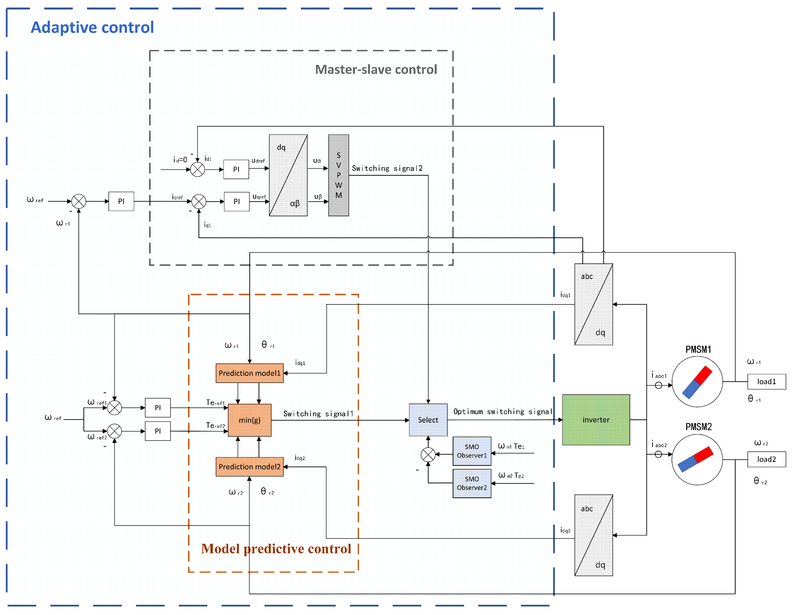
The overall system control block diagram is shown in Figure 4.

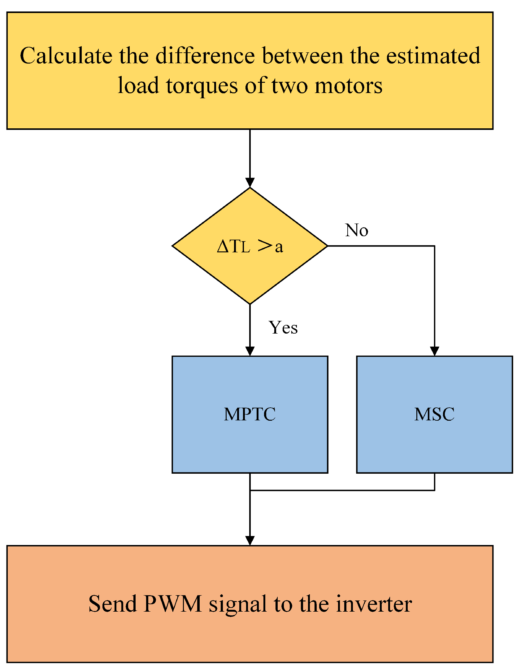
Given the reference speed, the outer speed loop is regulated by a proportional-integral (PI) controller. In the inner loop, an adaptive controller selects the appropriate control strategy according to the estimated load condition. Specifically, the load-torque difference between the two motors is obtained through a load-torque sliding mode observer, and the control mode is switched according to the threshold parameter a. When $\Delta T_L>a$, model predictive torque control (MPTC) is activated. When $\Delta T_L<a$, master–slave control (MSC) is employed. The corresponding switching process is illustrated in Figure 5.

3.1. Sliding Mode Observer of Load Torque

To estimate the load torque of the two motors, a sliding mode observer is first designed. The electromagnetic torque equation and the mechanical motion equation of the motor are written as follows:

$$T_e=1.5P_n\left[{\psi }_f{i}_q+\left(L_d-L_q\right)i_d{i}_q\right]$$

(31)

$$J{\displaystyle \frac{d{\omega }_r}{dt}}=T_e-B{\omega }_r-T_L$$

(32)

Here, $P_n$ represents the number of motor poles, ${\psi }_f$ denotes the permanent-magnet flux linkage, ${\omega }_r$ is the angular velocity, J is the moment of inertia, B is the viscous friction coefficient, $T_e$ is the electromagnetic torque, and $T_L$ is the load torque.

The state equations of the PMSM can therefore be expressed as

$$\left\{\begin{array}{c}\hfill {\displaystyle \frac{d{\omega }_e}{dt}}={\displaystyle \frac{1.5P_n}{2J}}\left[{\psi }_f{i}_q+\left(L_d-L_q\right)i_d{i}_q\right]-{\displaystyle \frac{P_n}{J}}{T}_L-{\displaystyle \frac{B}{J}}{\omega }_e,\\ {\dot{T}}_L=0.\hfill \end{array}\right.$$

(33)

Since the electrical time constant is much smaller than the mechanical time constant, the load torque can be assumed to remain constant within one control period [36]. Under this assumption, the observer-based velocity estimation can be written as

$${\displaystyle \frac{d{\widehat{\omega }}_e}{dt}}={\displaystyle \frac{1.5P_n}{2J}}\left[{\psi }_f{i}_q+\left(L_d-L_q\right)i_d{i}_q\right]-{\displaystyle \frac{B}{J}}{\widehat{\omega }}_e-Z_s$$

(34)

where ${\widehat{\omega }}_e$ is the estimated electrical angular velocity, and

$$Z_s=k\mathrm{sign}\left({\widehat{\omega }}_e-{\omega }_e\right)$$

(35)

is the switching signal defined by the sign function, with k denoting the sliding-mode gain.

Define the velocity estimation error as

$${\omega }_{ee}={\widehat{\omega }}_e-{\omega }_e.$$

(36)

Subtracting the speed equation in Equation (33) from Equation (34) yields

$${\displaystyle \frac{d{\omega }_{ee}}{dt}}={\displaystyle \frac{P_n}{J}}{T}_L-{\displaystyle \frac{B}{J}}{\omega }_{ee}-Z_s$$

(37)

The sliding surface is defined as

$$s\left(x\right)=\sigma ={\widehat{\omega }}_e-{\omega }_e.$$

(38)

According to sliding mode control theory, when the system reaches the sliding surface, that is, when $s\left(x\right)=0$, the estimated load torque can be expressed as [37]

$${\widehat{T}}_L={\displaystyle \frac{J}{P_n}}{Z}_s.$$

(39)

Because of the discontinuity of the switching function, the estimated load torque contains high-frequency noise, which can be described as

$${\widehat{T}}_L=T_L+\Delta u_s.$$

(40)

Here, $\Delta u_s$ represents the high-frequency noise caused by the discontinuous switching action, which may lead to system chattering. To obtain a smoother load-torque estimate, a first-order low-pass filter (LPF) is introduced, and the filtered estimate is given by

$${\widehat{T}}_L={\displaystyle \frac{J}{P_n}}{Z}_s·{\displaystyle \frac{{\omega }_c}{s+{\omega }_c}}$$

(41)

where ${\omega }_c$ is the cutoff frequency of the LPF. Alternatively, the sign function may be replaced by a sigmoid or saturation function to further improve smoothness.

The stability of the sliding mode observer is analyzed according to the convergence condition $s\dot{s}\le 0$ for generalized sliding motion [38]. From Equation (37), one has

$$s\dot{s}={\omega }_{ee}{\dot{\omega }}_{ee}={\omega }_{ee}\left[{\displaystyle \frac{P_n}{J}}{T}_L-{\displaystyle \frac{B}{J}}{\omega }_{ee}-k\mathrm{sgn}\left({\omega }_{ee}\right)\right]\le 0.$$

(42)

Since $-{\displaystyle \frac{B}{J}}{\omega }_{ee}^2\le 0$, a sufficient condition for satisfying the convergence requirement is

$$k\ge \left|{\displaystyle \frac{P_n}{J}}{T}_L\right|.$$

(43)

Robustness and Bandwidth Analysis of the Load-Torque Observer

The preceding observer design is derived under nominal motor parameters. In practical operation, however, the mechanical and electromagnetic parameters may deviate from their nominal values because of temperature variation, magnetic saturation, manufacturing tolerance, and load-dependent operating conditions. Therefore, the parameter uncertainties are considered as

$$J=J_0+\Delta J,B=B_0+\Delta B,{\psi }_f={\psi }_{f0}+\Delta {\psi }_f,L_d=L_{d0}+\Delta L_d,L_q=L_{q0}+\Delta L_q,$$

(44)

where the subscript 0 denotes the nominal value and $\Delta (·)$ denotes the corresponding parameter perturbation.

Considering the above uncertainties, the speed estimation error dynamics can be rewritten as

$${\dot{\omega }}_{ee}=-{\displaystyle \frac{B_0}{J_0}}{\omega }_{ee}+{\displaystyle \frac{P_n}{J_0}}{T}_L+d_{\omega }\left(t\right)-k\mathrm{sat}\left({\displaystyle \frac{{\omega }_{ee}}{\varphi }}\right),$$

(45)

where $d_{\omega }\left(t\right)$ denotes the lumped uncertainty caused by parameter mismatch, unmodeled dynamics, discretization error, and measurement noise. The saturation function $\mathrm{sat}(·)$ is used instead of the ideal sign function to reduce chattering, and $\varphi$ is the boundary-layer thickness.

Assume that the lumped uncertainty and load torque are bounded as

$$|d_{\omega }\left(t\right)|\le D_{\omega },\left|T_L\right|\le T_{L,max}.$$

(46)

The Lyapunov function is selected as

$$V={\displaystyle \frac{1}{2}}{\omega }_{ee}^2.$$

(47)

Outside the boundary layer, namely $|{\omega }_{ee}|>\varphi$, the saturation function satisfies $\mathrm{sat}({\omega }_{ee}/\varphi )=\mathrm{sgn}\left({\omega }_{ee}\right)$. Therefore,

$$\dot{V}={\omega }_{ee}\left[-{\displaystyle \frac{B_0}{J_0}}{\omega }_{ee}+{\displaystyle \frac{P_n}{J_0}}{T}_L+d_{\omega }\left(t\right)-k\mathrm{sgn}\left({\omega }_{ee}\right)\right].$$

(48)

A sufficient condition for satisfying the reaching condition $\dot{V}<0$ is

$$k>{\displaystyle \frac{P_n}{J_0}}{T}_{L,max}+D_{\omega }+\eta ,\eta >0,$$

(49)

where $\eta$ is a positive stability margin. Compared with the nominal gain condition, the revised condition explicitly considers both the bounded load torque and the lumped modeling uncertainty. Thus, increasing k improves robustness against parameter mismatch and external disturbance. However, an excessively large k may intensify chattering and increase the filtering burden of the low-pass filter. Therefore, the observer gain should be selected by considering both robustness and chattering suppression.

The first-order low-pass filter used for load-torque estimation is given by

$$G_{\mathrm{LPF}}\left(s\right)={\displaystyle \frac{{\omega }_c}{s+{\omega }_c}},$$

(50)

where ${\omega }_c$ is the cutoff frequency. Its magnitude response and phase response are

$$|G_{\mathrm{LPF}}\left(j\omega \right)|={\displaystyle \frac{{\omega }_c}{\sqrt{{\omega }^2+{\omega }_c^2}}},$$

(51)

$$\angle G_{\mathrm{LPF}}\left(j\omega \right)=-arctan\left({\displaystyle \frac{\omega }{{\omega }_c}}\right).$$

(52)

For a load-torque component with angular frequency ${\omega }_d$, the corresponding phase lag is

$${\phi }_d=arctan\left({\displaystyle \frac{{\omega }_d}{{\omega }_c}}\right),$$

(53)

and the equivalent phase-delay time can be approximated as

$$t_d={\displaystyle \frac{{\phi }_d}{{\omega }_d}}={\displaystyle \frac{1}{{\omega }_d}}arctan\left({\displaystyle \frac{{\omega }_d}{{\omega }_c}}\right).$$

(54)

The group delay of the filter is

$${\tau }_g\left(\omega \right)={\displaystyle \frac{{\omega }_c}{{\omega }_c^2+{\omega }^2}}.$$

(55)

These equations show that a larger ${\omega }_c$ reduces the phase delay and improves the response speed of the estimated load torque, whereas a smaller ${\omega }_c$ provides stronger suppression of high-frequency chattering and measurement noise. Therefore, ${\omega }_c$ determines the trade-off between estimation delay and estimation smoothness.

If the maximum allowable phase lag at the dominant load-disturbance frequency ${\omega }_d$ is ${\phi }_{max}$, the cutoff frequency should satisfy

$${\omega }_c\ge {\displaystyle \frac{{\omega }_d}{tan\left({\phi }_{max}\right)}}.$$

(56)

In addition, if the allowable amplitude attenuation is $\epsilon$, namely $|G_{\mathrm{LPF}}\left(j{\omega }_d\right)|\ge 1-\epsilon$, then

$${\omega }_c\ge {\displaystyle \frac{{\omega }_d}{\sqrt{\frac{1}{{(1-\epsilon )}^2}-1}}}.$$

(57)

Consequently, the cutoff frequency should be selected as

$${\omega }_c\ge max\left\{{\displaystyle \frac{{\omega }_d}{tan\left({\phi }_{max}\right)}},{\displaystyle \frac{{\omega }_d}{\sqrt{\frac{1}{{(1-\epsilon )}^2}-1}}}\right\}.$$

(58)

From the above analysis, the load-torque estimation accuracy is mainly affected by three factors: the boundary-layer thickness $\varphi$, the lumped uncertainty bound $D_{\omega }$, and the cutoff frequency ${\omega }_c$. A smaller $\varphi$ can improve the steady-state estimation accuracy but may increase chattering. A larger ${\omega }_c$ can reduce the estimation delay but may allow more high-frequency switching components to pass through. Therefore, the observer gain k, boundary-layer thickness $\varphi$, and cutoff frequency ${\omega }_c$ should be jointly selected to achieve a compromise among robustness, estimation delay, and chattering suppression. This analytical bandwidth and phase-delay discussion provides a quantitative basis for the use of the low-pass filter, rather than introducing it in an ad hoc manner.

3.2. Adaptive Controller

PI controllers are employed in the current vector control system. By applying the corresponding coordinate transformation to Equation (1), the relationship between the current derivative and the voltage can be written as

$$\left\{\begin{array}{cc}\hfill {\displaystyle \frac{d{i}_d}{dt}}& ={\displaystyle \frac{u_d-R{i}_d+{\omega }_e{L}_q{i}_q}{L_d}},\hfill \\ \hfill {\displaystyle \frac{d{i}_q}{dt}}& ={\displaystyle \frac{u_q-R{i}_q-{\omega }_e\left(L_d{i}_d+{\psi }_f\right)}{L_q}}.\hfill \end{array}\right.$$

(59)

Equation (59) can be discretized as

$$\left\{\begin{array}{cc}\hfill {\displaystyle \frac{i_d(k+1)-i_d\left(k\right)}{T_s}}& ={\displaystyle \frac{u_d\left(k\right)-R{i}_d\left(k\right)+{\omega }_e\left(k\right)L_q{i}_q\left(k\right)}{L_d}},\hfill \\ \hfill {\displaystyle \frac{i_q(k+1)-i_q\left(k\right)}{T_s}}& ={\displaystyle \frac{u_q\left(k\right)-R{i}_q\left(k\right)-{\omega }_e\left(k\right)\left(L_d{i}_d\left(k\right)+{\psi }_f\right)}{L_q}}.\hfill \end{array}\right.$$

(60)

Using Equation (60), the current at time $k+1$ can be predicted from the state at time k, and the corresponding torque and flux at time $k+1$ can then be calculated as

$$T_e(k+1)=1.5P_n{i}_q(k+1)\left[i_d(k+1)\left(L_d-L_q\right)+{\psi }_f\right]$$

(61)

$$\left\{\begin{array}{cc}\hfill {\psi }_d(k+1)& =L_d{i}_d(k+1)+{\psi }_f,\hfill \\ \hfill {\psi }_q(k+1)& =L_q{i}_q(k+1).\hfill \end{array}\right.$$

(62)

$${\psi }_s(k+1)=\sqrt{{\psi }_d^2(k+1)+{\psi }_q^2(k+1)}.$$

(63)

To make the predicted torque and flux track their reference values, the switching state is selected online by minimizing a cost function. In conventional FCS-MPTC, torque error and stator-flux error have different physical units and numerical ranges. If these terms are directly added together, the selection of the weighting coefficient becomes empirical and case-dependent. Therefore, a normalized cost function is adopted in this study:

$$\begin{array}{cc}\hfill g_i=& {\displaystyle \frac{\left|T_{e1}^{*}-T_{e1}^p(k+1)\right|}{T_N}}+{\lambda }_{\psi }{\displaystyle \frac{\left|{\psi }_{s1}^{*}-{\psi }_{s1}^p(k+1)\right|}{{\psi }_N}}\hfill \\ \hfill & +{\displaystyle \frac{\left|T_{e2}^{*}-T_{e2}^p(k+1)\right|}{T_N}}+{\lambda }_{\psi }{\displaystyle \frac{\left|{\psi }_{s2}^{*}-{\psi }_{s2}^p(k+1)\right|}{{\psi }_N}},i=1,2,3,\dots ,N_v.\hfill \end{array}$$

(64)

Here, $T_{e1}$ and $T_{e2}$ denote the electromagnetic torques of motors 1 and 2, respectively, while ${\psi }_{s1}$ and ${\psi }_{s2}$ denote their corresponding stator flux magnitudes. The superscript p denotes the predicted value at time $k+1$, and $N_v$ is the number of candidate voltage vectors evaluated in the predictive control mode. $T_N$ and ${\psi }_N$ are the normalization bases for torque and stator flux, respectively.

To suppress the fluctuation of the d-axis current, the normalized d-axis current term is further incorporated into the cost function:

$$\begin{array}{cc}\hfill g_i=& {\displaystyle \frac{\left|T_{e1}^{*}-T_{e1}^p(k+1)\right|}{T_N}}+{\lambda }_{\psi }{\displaystyle \frac{\left|{\psi }_{s1}^{*}-{\psi }_{s1}^p(k+1)\right|}{{\psi }_N}}\hfill \\ \hfill & +{\displaystyle \frac{\left|T_{e2}^{*}-T_{e2}^p(k+1)\right|}{T_N}}+{\lambda }_{\psi }{\displaystyle \frac{\left|{\psi }_{s2}^{*}-{\psi }_{s2}^p(k+1)\right|}{{\psi }_N}}\hfill \\ \hfill & +{\lambda }_d{\displaystyle \frac{\left|i_{d1}^p(k+1)\right|}{I_N}}+{\lambda }_d{\displaystyle \frac{\left|i_{d2}^p(k+1)\right|}{I_N}},i=1,2,3,\dots ,N_v.\hfill \end{array}$$

(65)

Here, $i_{d1}$ and $i_{d2}$ denote the d-axis currents of motors 1 and 2, respectively. $I_N$ is the normalization base for the current term. In this study, the normalization bases are selected as

$$T_N=T_{\mathrm{rated}},{\psi }_N={\psi }_f,I_N=I_{\mathrm{rated}}.$$

(66)

After normalization, all terms in the cost function become dimensionless. Therefore, the weighting factors ${\lambda }_{\psi }$ and ${\lambda }_d$ are used to adjust the relative priority among torque tracking, stator-flux regulation, and d-axis current suppression, rather than to compensate for different physical units. This avoids the direct addition of variables with different dimensions and reduces the arbitrariness of weighting-factor selection. When ${\lambda }_d=0$, the cost function degenerates into the conventional torque-and-flux predictive control form. When ${\lambda }_d>0$, the d-axis current suppression term is activated to reduce d-axis current fluctuation and improve the three-phase current waveform quality.

The weighting factors are selected according to a sequential tuning procedure. First, ${\lambda }_{\psi }$ is tuned while setting ${\lambda }_d=0$, so that the stator flux error remains within an acceptable range without significantly slowing down the torque response. Then, ${\lambda }_d$ is gradually increased from zero to suppress the d-axis current ripple and improve the three-phase current waveform. Finally, the selected weighting factors are checked under load-step conditions to ensure that the speed overshoot and settling time remain acceptable. In practical tuning, the final values of ${\lambda }_{\psi }$ and ${\lambda }_d$ are selected by considering the compromise among speed overshoot, settling time, d-axis current ripple, and torque ripple:

$$min\{M_p,t_s,\Delta i_d,\Delta T_e\},$$

(67)

where $M_p$ is the speed overshoot, $t_s$ is the settling time, $\Delta i_d$ is the d-axis current ripple, and $\Delta T_e$ is the torque ripple. After this tuning procedure, the selected weighting factors are fixed and kept unchanged in all subsequent load-disturbance simulations to ensure a fair comparison among different control strategies.

The output of the PI controller is given by

$$u\left(t\right)=K_{p}e\left(t\right)+K_i{\int }_0^{t}e\left(\tau \right)d\tau ,$$

(68)

where $e\left(t\right)=r\left(t\right)-y\left(t\right)$ is the instantaneous error, $r\left(t\right)$ is the reference input, $y\left(t\right)$ is the measured output, and $K_p$ and $K_i$ are the proportional and integral gains, respectively. Its discrete-time form can be written as

$$u\left(k\right)=K_{p}e\left(k\right)+K_i{T}_s{\displaystyle \sum _{j=0}^k}e\left(j\right).$$

(69)

Here, $T_s$ is the sampling period, and ${\sum }_{j=0}^{k}e\left(j\right)$ is the cumulative error. In each control cycle, the PI controller only requires the computation of the proportional term, the integral term, and the accumulation operation. By contrast, FCS-MPTC requires online prediction and evaluation of candidate voltage vectors.

In the proposed adaptive control strategy, predictive torque control is not activated during balanced or weakly unbalanced load conditions. When the estimated load-torque difference satisfies $\Delta T_L<a$, the controller operates in vector-control mode, and the online enumeration of finite voltage vectors is bypassed. When $\Delta T_L\ge a$, FCS-MPTC is activated, and the candidate voltage vectors are evaluated according to the normalized cost function.

Therefore, compared with full-time finite-set model predictive torque control, the proposed method reduces the average number of predictive evaluations over a complete operating period.

It should be noted that the proposed method does not reduce the candidate voltage-vector set inside the active predictive control mode. Instead, the reduction in computational effort comes from the conditional activation of finite-set model predictive torque control according to the estimated load imbalance. If the total number of control cycles is denoted by $N_{\mathrm{tot}}$, and the number of cycles in which finite-set model predictive torque control is activated is denoted by $N_{\mathrm{MPC}}$, the total number of voltage-vector evaluations for full-time finite-set model predictive torque control and the proposed adaptive strategy can be expressed as

$$N_{\mathrm{eval}}^{\mathrm{full}}=N_v{N}_{\mathrm{tot}},N_{\mathrm{eval}}^{\mathrm{pro}}=N_v{N}_{\mathrm{MPC}}.$$

(70)

Accordingly, the reduction ratio of predictive evaluations is

$${\eta }_{\mathrm{eval}}={\displaystyle \frac{N_{\mathrm{eval}}^{\mathrm{full}}-N_{\mathrm{eval}}^{\mathrm{pro}}}{N_{\mathrm{eval}}^{\mathrm{full}}}}\times 100\%=\left(1-{\displaystyle \frac{N_{\mathrm{MPC}}}{N_{\mathrm{tot}}}}\right)\times 100\%.$$

(71)

This formulation clarifies that the computational reduction is achieved by avoiding unnecessary full-time predictive optimization under balanced or weakly unbalanced load conditions, while the standard candidate voltage-vector set is retained when predictive torque control is active.

4. Simulation Analysis

4.1. Simulation Setup and Controller Parameters

To verify the effectiveness of the proposed adaptive control strategy, simulations were carried out in Matlab/Simulink R2021b (version 9.11.0.1769968, 64-bit, Windows, released on 17 September 2021). The motor parameters used in the simulations are listed in

Table 2. Parameters of PMSM.

Parameter	Value
Rated power P/kW	3
Rated load $T_L$/N·m	23.875
Rated speed $N_r$/rpm	1200
Stator resistance $R_s$/$\Omega$	0.958
Stator inductance L/H	0.000835
Permanent magnet flux linkage $\psi$/Wb	0.1827
Moment of inertia J/kg·m2	0.003
Damping coefficient B/N·m·s	0.008
Number of poles	4

.

To improve the reproducibility of the proposed control scheme, the main controller parameters used in the simulations are listed in

Table 3. Main controller parameters used in the simulations.

Control Part	Parameter	Value
MSC speed-loop PI	$K_{p\omega }$, $K_{i\omega }$,	0.2, 30
MSC current-loop PI	$K_{pid}$, $K_{iid}$, $K_{piq}$, $K_{iiq}$	300, 23,950, 300, 23,950
MPTC speed-loop PI	$K_{p\omega }$, $K_{i\omega }$	0.2, 30
MPTC cost function	${\lambda }_{\psi }$, ${\lambda }_d$	0.05, 0.001
Adaptive switching	a	0.5 N·m

. The PI controller parameters were first tuned to obtain stable speed and current responses under the vector-control mode, and then kept unchanged in all comparative simulations. In the predictive torque control mode, the same speed-loop PI parameters were used. The stator-flux weighting factor ${\lambda }_{\psi }$ and the d-axis current suppression weighting factor ${\lambda }_d$ were selected by considering the compromise among torque tracking, flux regulation, current ripple suppression, and transient speed response. The adaptive switching threshold a was selected according to the estimated load-torque difference and was set to 0.5 N·m in the simulations. All controller parameters listed in Table 3 were kept unchanged for different comparative control strategies to ensure a fair comparison.

4.2. Mathematical Formulations of Comparative Control Strategies

To improve the clarity of the comparative simulations, the mathematical formulations of the main control strategies used in Section 4 are summarized in this subsection. The compared methods include conventional master–slave control, improved master–slave control, average model control, conventional MPTC, improved MPTC, and the proposed adaptive control strategy.

For the conventional master–slave control, motor 1 is fixed as the master motor, whereas motor 2 operates as the slave motor. The speed-loop error of the master motor is defined as

$$e_{\omega 1}\left(k\right)={\omega }^{*}\left(k\right)-{\omega }_1\left(k\right),$$

(72)

and the reference q-axis current is generated by the speed-loop PI controller as

$$i_{q1}^{*}\left(k\right)=K_{p\omega }{e}_{\omega 1}\left(k\right)+K_{i\omega }{T}_s{\displaystyle \sum _{j=0}^k}{e}_{\omega 1}\left(j\right),$$

(73)

where ${\omega }^{*}$ is the reference speed, ${\omega }_1$ is the speed of motor 1, and $T_s$ is the sampling period. The d-axis current reference is set as

$$i_{d1}^{*}\left(k\right)=0.$$

(74)

The current-loop errors are given by

$$e_{d1}\left(k\right)=i_{d1}^{*}\left(k\right)-i_{d1}\left(k\right),e_{q1}\left(k\right)=i_{q1}^{*}\left(k\right)-i_{q1}\left(k\right).$$

(75)

Then, the voltage references are generated by the current-loop PI controllers:

$$\left\{\begin{array}{c}{u}_{d1}^{*}\left(k\right)=K_{pid}{e}_{d1}\left(k\right)+K_{iid}{T}_s{\displaystyle {\sum }_{j=0}^k}{e}_{d1}\left(j\right),\hfill \\ u_{q1}^{*}\left(k\right)=K_{piq}{e}_{q1}\left(k\right)+K_{iiq}{T}_s{\displaystyle {\sum }_{j=0}^k}{e}_{q1}\left(j\right).\hfill \end{array}\right.$$

(76)

The obtained voltage vector is applied to the common inverter through SVPWM. Since the two motors share the same inverter, the same voltage vector is simultaneously applied to both motors.

For the improved master–slave control, the motor subjected to the larger estimated load torque is selected as the feedback motor for voltage-vector generation. The master motor index is defined as

$$m=arg\underset{j=1,2}{max}\left({\widehat{T}}_{Lj}\right),$$

(77)

where ${\widehat{T}}_{Lj}$ is the estimated load torque of motor j. The corresponding speed-loop error is

$$e_{\omega m}\left(k\right)={\omega }^{*}\left(k\right)-{\omega }_m\left(k\right),$$

(78)

and the current reference is calculated as

$$i_{qm}^{*}\left(k\right)=K_{p\omega }{e}_{\omega m}\left(k\right)+K_{i\omega }{T}_s{\displaystyle \sum _{j=0}^k}{e}_{\omega m}\left(j\right),i_{dm}^{*}\left(k\right)=0.$$

(79)

The voltage vector is then generated by the current-loop PI controllers of the selected master motor. This strategy improves the fixed master–slave control by adjusting the feedback object according to the load condition.

For the average model control, the dual-motor system is treated as an equivalent single controlled object. The average speed and average currents are defined as

$${\omega }_{\mathrm{avg}}={\displaystyle \frac{{\omega }_1+{\omega }_2}{2}},i_{d,\mathrm{avg}}={\displaystyle \frac{i_{d1}+i_{d2}}{2}},i_{q,\mathrm{avg}}={\displaystyle \frac{i_{q1}+i_{q2}}{2}}.$$

(80)

The speed-loop error is expressed as

$$e_{\omega ,\mathrm{avg}}\left(k\right)={\omega }^{*}\left(k\right)-{\omega }_{\mathrm{avg}}\left(k\right),$$

(81)

and the reference currents are obtained as

$$i_{q,\mathrm{avg}}^{*}\left(k\right)=K_{p\omega }{e}_{\omega ,\mathrm{avg}}\left(k\right)+K_{i\omega }{T}_s{\displaystyle \sum _{j=0}^k}{e}_{\omega ,\mathrm{avg}}\left(j\right),i_{d,\mathrm{avg}}^{*}\left(k\right)=0.$$

(82)

The voltage reference is generated according to the average current errors:

$$e_{d,\mathrm{avg}}=i_{d,\mathrm{avg}}^{*}-i_{d,\mathrm{avg}},e_{q,\mathrm{avg}}=i_{q,\mathrm{avg}}^{*}-i_{q,\mathrm{avg}}.$$

(83)

For the conventional MPTC, the candidate voltage vector is selected by minimizing the torque and stator-flux tracking errors of the two motors. Based on the prediction model, the conventional cost function is written as

$$\begin{array}{cc}\hfill g_i^{\mathrm{con}}=& {\left(T_{e1}^{*}-T_{e1}^p(k+1)\right)}^2+{\lambda }_{\psi }{\left({\psi }_{s1}^{*}-{\psi }_{s1}^p(k+1)\right)}^2\hfill \\ \hfill & +{\left(T_{e2}^{*}-T_{e2}^p(k+1)\right)}^2+{\lambda }_{\psi }{\left({\psi }_{s2}^{*}-{\psi }_{s2}^p(k+1)\right)}^2,i=1,2,\dots ,N_v,\hfill \end{array}$$

(84)

where $T_{e1}^p$ and $T_{e2}^p$ are the predicted electromagnetic torques, ${\psi }_{s1}^p$ and ${\psi }_{s2}^p$ are the predicted stator-flux magnitudes, ${\lambda }_{\psi }$ is the stator-flux weighting factor, and $N_v$ is the number of candidate voltage vectors. The optimal voltage vector is determined by

$$u_{\mathrm{opt}}\left(k\right)=arg\underset{u_i\in \mathcal{V}}{min}{g}_i^{\mathrm{con}},$$

(85)

where $\mathcal{V}$ denotes the finite candidate voltage-vector set.

For the improved MPTC, a d-axis current suppression term is further introduced into the cost function to improve the current waveform quality:

$$\begin{array}{cc}\hfill g_i^{\mathrm{imp}}=& g_i^{\mathrm{con}}+{\lambda }_d{\left(i_{d1}^p(k+1)\right)}^2+{\lambda }_d{\left(i_{d2}^p(k+1)\right)}^2,i=1,2,\dots ,N_v,\hfill \end{array}$$

(86)

where ${\lambda }_d$ is the d-axis current suppression weighting factor. In this study, ${\lambda }_{\psi }=0.05$ and ${\lambda }_d=0.002$ were used in the predictive-control simulations.

For the proposed adaptive control strategy, the estimated load-torque difference is used as the control-mode switching variable:

$$\Delta T_L=\left|{\widehat{T}}_{L1}-{\widehat{T}}_{L2}\right|.$$

(87)

The control law is expressed as

$$u\left(k\right)=\left\{\begin{array}{cc}{u}_{\mathrm{MSC}}\left(k\right),\hfill & \Delta T_L<a,\hfill \\ u_{\mathrm{MPTC}}^{\mathrm{imp}}\left(k\right),\hfill & \Delta T_L\ge a,\hfill \end{array}\right.$$

(88)

where $u_{\mathrm{MSC}}\left(k\right)$ denotes the voltage vector generated by the master–slave vector control mode, $u_{\mathrm{MPTC}}^{\mathrm{imp}}\left(k\right)$ denotes the voltage vector selected by the improved MPTC cost function, and a is the load-difference threshold. In the simulations, $a=0.5$ N·m.

The switching threshold a is a key parameter in the proposed adaptive control law, because it determines whether the controller operates in the master–slave vector control mode or in the improved MPTC mode. Therefore, a should not be regarded as a purely empirical constant. In practical implementation, its selection should consider the estimation fluctuation of the load-torque observer, the rated load torque, and the maximum load imbalance that can still be tolerated by the master–slave control mode.

First, a should be larger than the steady-state fluctuation of the estimated load-torque difference under balanced or weakly unbalanced load conditions. Otherwise, small observer noise, measurement noise, or filtering-induced fluctuation may cause unnecessary switching between the two control modes. Thus, the lower bound of a can be expressed as

$$a_{min}=\Delta T_{\mathrm{obs}}+\Delta T_{\mathrm{m}},$$

(89)

where $\Delta T_{\mathrm{obs}}$ denotes the maximum steady-state fluctuation of the estimated load-torque difference, and $\Delta T_{\mathrm{m}}$ is a safety margin used to prevent false switching.

Second, a should be smaller than the critical load-torque difference at which the master–slave control mode can no longer maintain acceptable dynamic performance. This critical value can be determined by gradually increasing the load-torque difference and observing whether the speed synchronization error, speed overshoot, settling time, or current ripple exceeds the allowable limit. The corresponding upper bound is defined as

$$a_{max}=\Delta T_{\mathrm{crit}},$$

(90)

where $\Delta T_{\mathrm{crit}}$ denotes the critical load-torque difference that the master–slave control mode can tolerate while still satisfying the required dynamic-performance indices.

Therefore, the practical tuning range of the switching threshold can be written as

$$a_{min}<a<a_{max}.$$

(91)

For motors with different rated load torques, the threshold can also be normalized as

$${\rho }_a={\displaystyle \frac{a}{T_{\mathrm{rated}}}},$$

(92)

where $T_{\mathrm{rated}}$ is the rated load torque. A smaller ${\rho }_a$ makes the controller more sensitive to load imbalance and activates the improved MPTC mode earlier, which improves disturbance rejection but increases the activation frequency of predictive optimization. By contrast, a larger ${\rho }_a$ keeps the system in the master–slave control mode for a longer time, which reduces the computational burden but may delay the activation of the improved MPTC mode under severe load imbalance.

In this study, the rated load torque is $23.875\mathrm{N}·\mathrm{m}$, and the switching threshold is selected as $a=0.5\mathrm{N}·\mathrm{m}$, corresponding to approximately $2.1\%$ of the rated load torque. This value is sufficiently larger than the steady-state fluctuation of the estimated load-torque difference, while allowing the improved MPTC mode to be activated before severe speed oscillation occurs under significant load imbalance. It should be noted that, because practical studies on single-inverter dual-PMSM systems are still relatively limited, the exact value of a may depend on motor parameters, observer bandwidth, measurement noise, load characteristics, and actual operating conditions. Therefore, the proposed tuning rule provides a systematic initial selection method, while further experimental calibration is still necessary for practical industrial applications.

4.3. Comparative Simulation Results

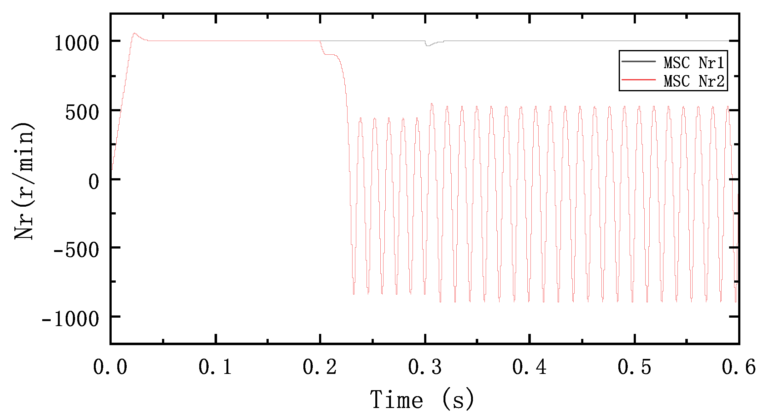
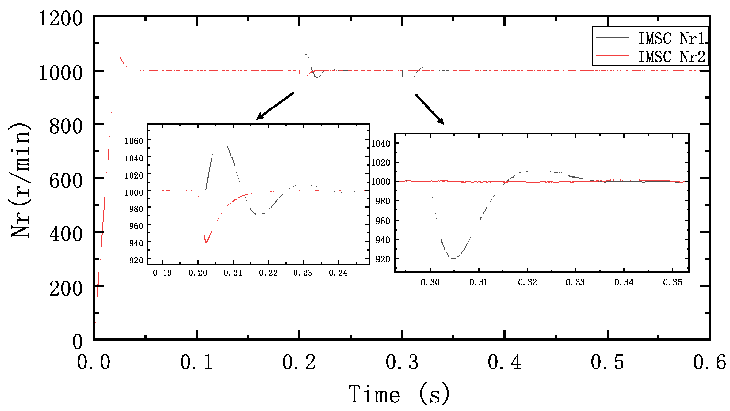
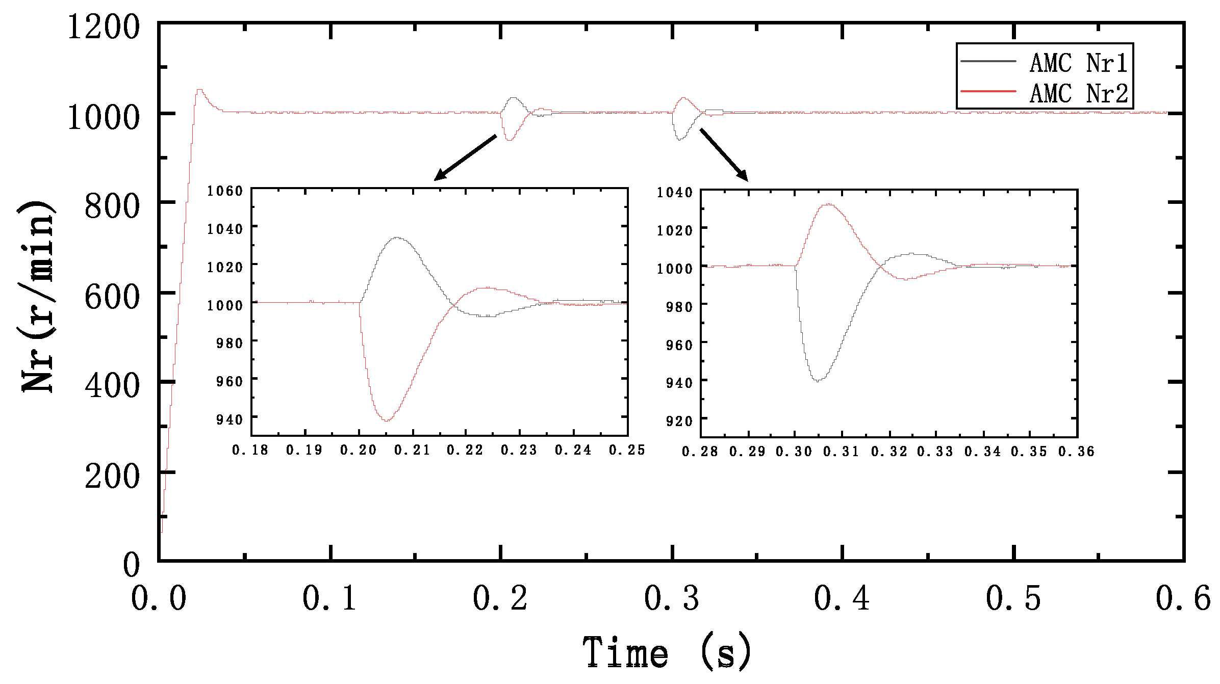
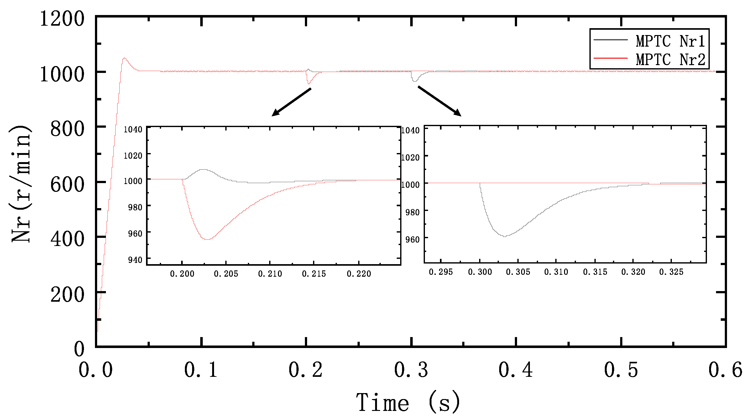
Two motors with identical parameters were considered. In the conventional master–slave control scheme, vector control with $i_d=0$ was adopted, where motor 1 acted as the master motor and motor 2 acted as the slave motor. The DC bus voltage was set to 311 V, and the reference speed was set to 1000 rpm. Initially, both motors operated under a load of 12 N·m. At 0.2 s, an additional load of 10 N·m was applied to motor 2, and at 0.3 s, an additional load of 10 N·m was applied to motor 1.

Figure 6 shows the speed response under conventional master–slave control. When the slave motor is subjected to a sudden load change, significant speed oscillation appears, which degrades the overall operating performance of the system.In this study, the improved master–slave control (MSC) refers to the master–slave vector control strategy with stability-oriented adjustment under load variation.

Figure 7 shows the speed responses of the two motors under the improved master–slave control (IMSC) strategy. The results indicate that the vector control-based strategy can maintain stable operation under abrupt load variation.

Under the master–slave control strategy, at 0.2 s, motor 1 started to respond at 0.2023 s and reached 1000.490 rpm at 0.2515 s, with an overshoot of 5.938%. Motor 2 started to respond at 0.2000 s and reached 1000.158 rpm at 0.228 s, with an overshoot of 6.182%. At 0.3 s, motor 1 started to respond at 0.3000 s and reached 1000.659 rpm at 0.3335 s, with an overshoot of 8.023%, while the speed of motor 2 remained between 998.933 rpm and 1002.043 rpm.

Figure 8 shows the speed response under average model control (AMC). The results indicate that AMC performs less effectively than predictive control under large load disturbance.

Under average model control, at 0.2 s, motor 1 started to respond at 0.20047 s and reached 1000.083 rpm at 0.235 s, with an overshoot of 3.383%. Motor 2 started to respond at 0.2000 s and reached 1000.645 rpm at 0.2334 s, with an overshoot of 6.216%. At 0.3 s, motor 1 started to respond at 0.3000 s and reached 1000.470 rpm at 0.3339 s, with an overshoot of 6.040%. Motor 2 started to respond at 0.3004 s and reached 1000.024 rpm at 0.3367 s, with an overshoot of 3.226%.

Figure 9 shows the speed response under conventional predictive torque control. Unlike master–slave control, this method does not require explicit distinction between the master motor and the slave motor.

Under conventional predictive torque control, at 0.2 s, motor 1 started to respond at 0.2000 s and reached 1000.0002 rpm at 0.2301 s, with an overshoot of 0.786%. Motor 2 started to respond at 0.20001 s and reached 1000.008 rpm at 0.236 s, with an overshoot of 4.611%. At 0.3 s, motor 1 started to respond at 0.3000098 s and reached 1000.0661 rpm at 0.3241 s, with an overshoot of 3.882%. The speed of motor 2 remained between 999.516 rpm and 1000.36 rpm.

In terms of dynamic performance, compared with master–slave control, the overshoot of motor 1 under conventional predictive torque control was reduced by 5.166% at 0.2 s, and the overshoot of motor 2 was reduced by 1.571%. At 0.3 s, the overshoot of motor 1 was reduced by 4.15%, and the deviation of motor 2 from the reference speed was reduced to 0.583–1.683 rpm. Compared with average model control, the response time of motor 1 was 0.035 s shorter at 0.2 s, and the overshoot of motor 2 was reduced by 1.605%. At 0.3 s, motor 1 still exhibited a small overshoot, while motor 2 maintained a more stable speed response.

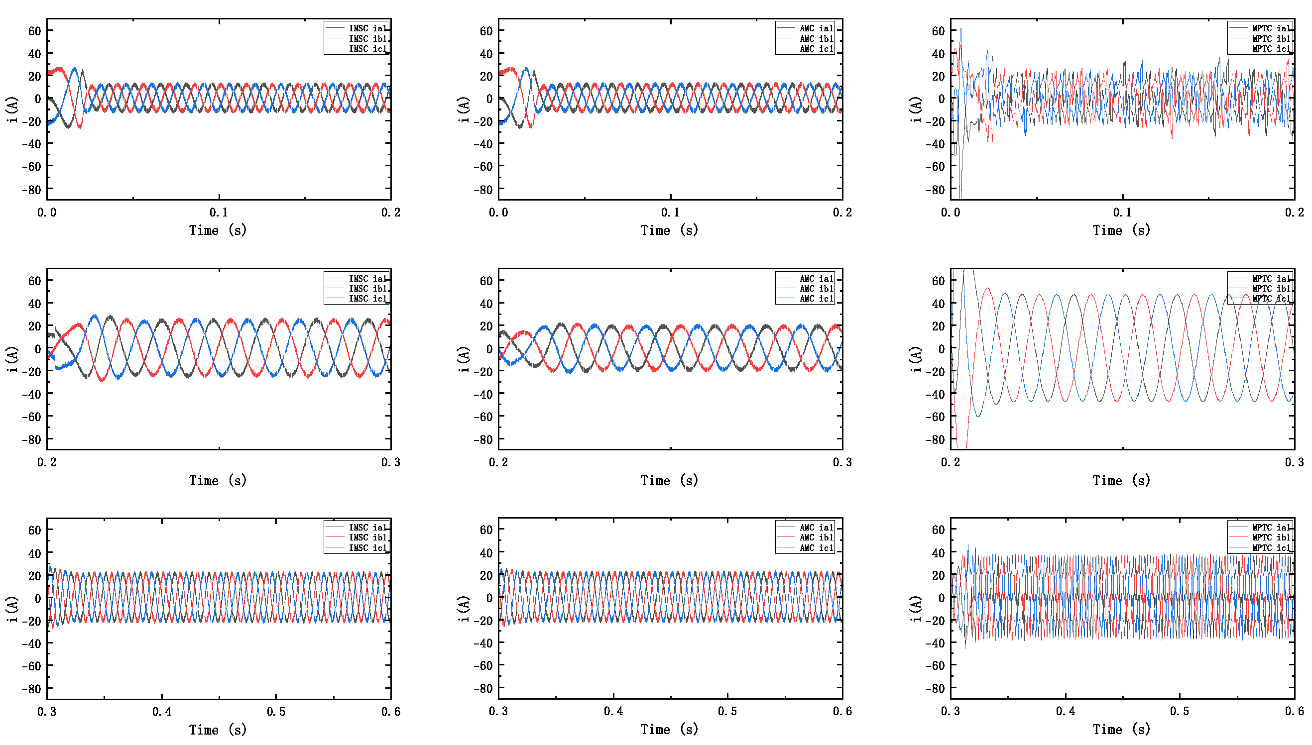
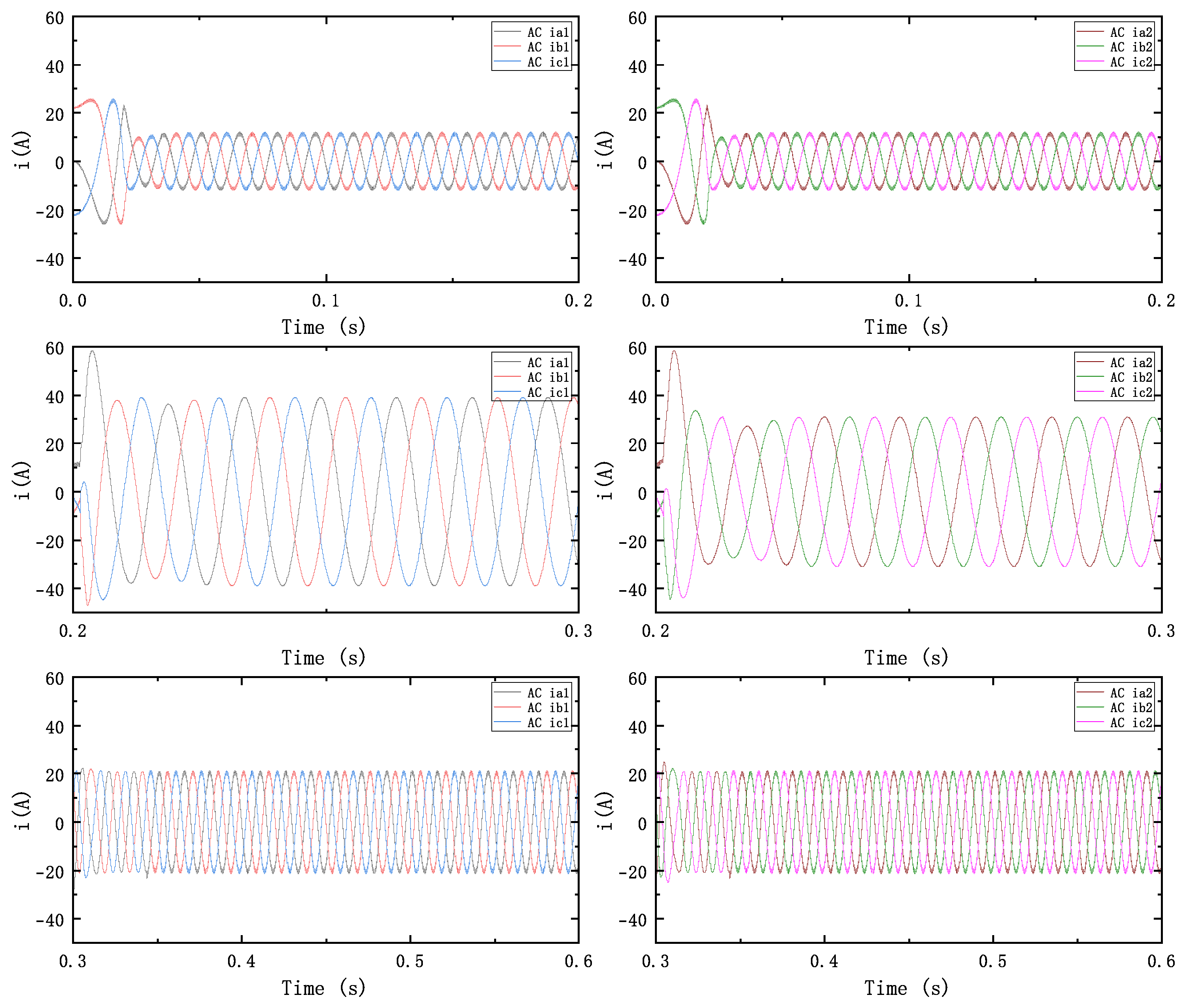
However, although conventional predictive torque control provides a fast dynamic response, the three-phase current waveform is relatively poor because the controller cannot directly regulate the current. Excessive current may lead to overheating and possible motor damage, as shown in Figure 10 and Figure 11.

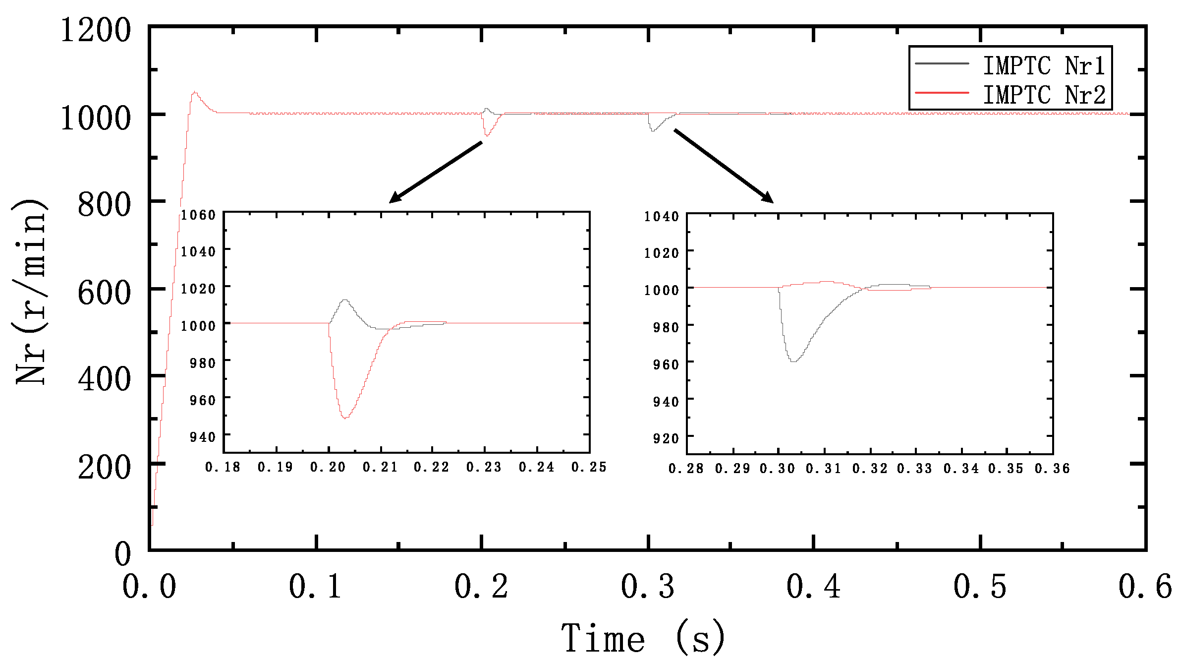
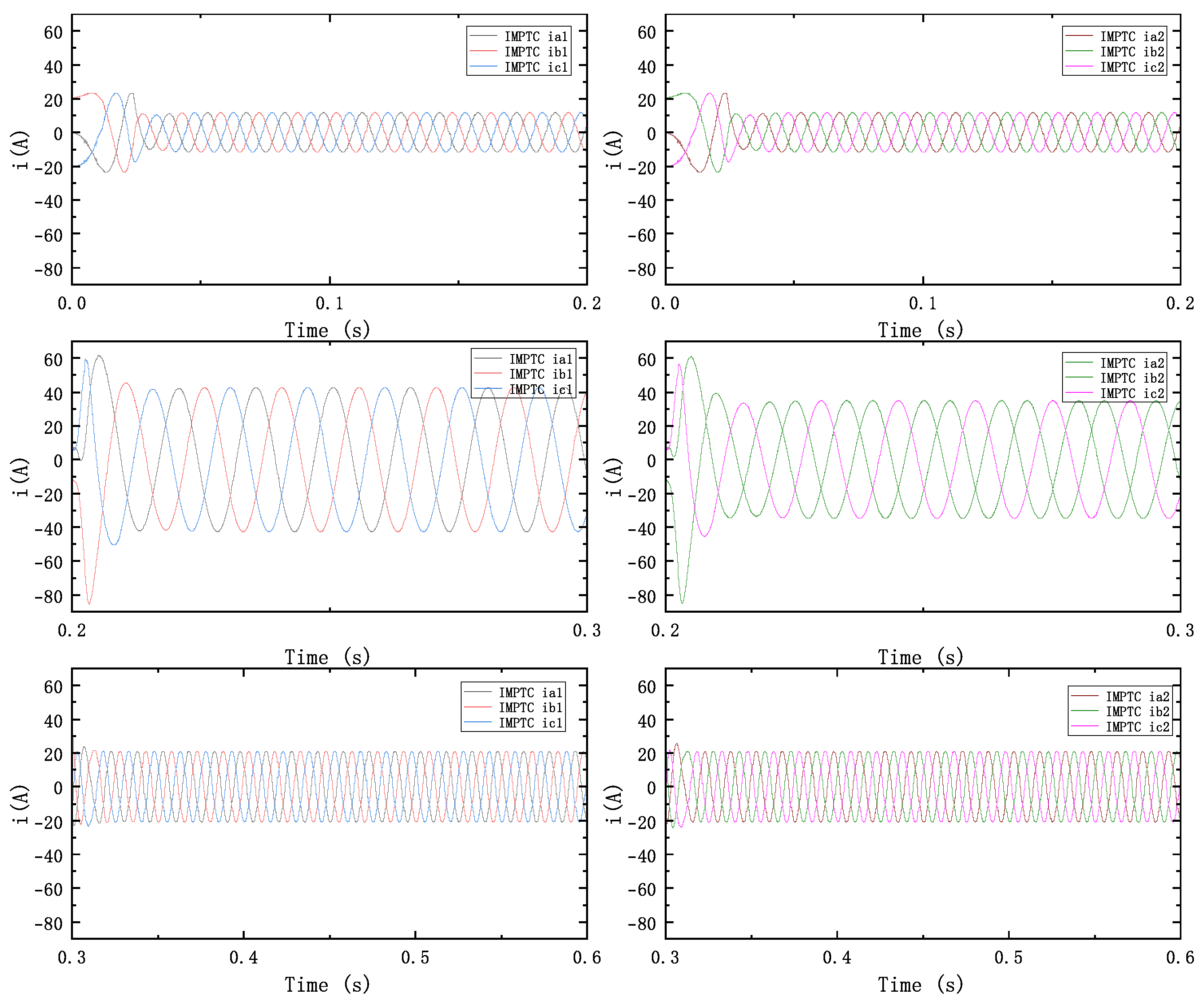
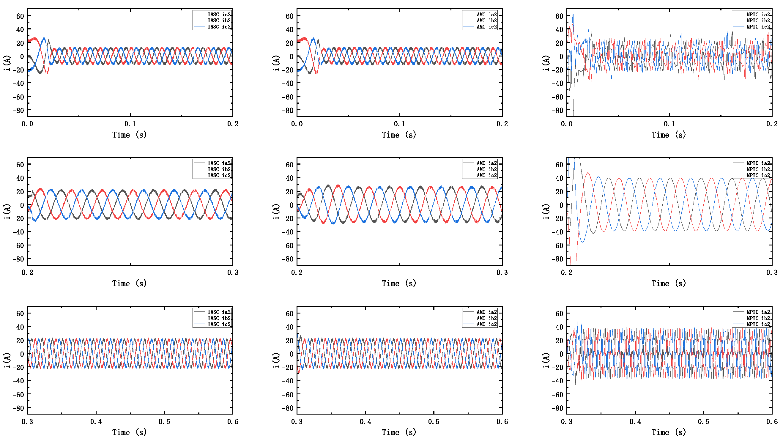
To improve the current waveform under predictive torque control (IMPTC), a d-axis current suppression term was introduced into the cost function, and its weighting coefficient was set to ${\lambda }_d=0.001$. The corresponding speed and three-phase current waveforms are shown in Figure 12 and Figure 13.

Under the improved finite-set predictive control strategy, at 0.2 s, the overshoot of motor 1 was 0.125%, whereas the overshoot of motor 2 was 5.137%. At 0.3 s, the overshoot of motor 1 was 4.028%, and the speed of motor 2 remained between 998.092 rpm and 1003.0597 rpm. These results indicate that the improved strategy significantly enhances the three-phase current waveform. The value of the d-axis current weighting coefficient ${\lambda }_d$ can be selected according to practical requirements. A larger value of ${\lambda }_d$ is beneficial for improving stability and reducing noise, whereas a smaller value of ${\lambda }_d$ is favorable for faster speed tracking.

In conventional predictive control, the cost function must be evaluated for all seven voltage vectors in each control cycle, and the switching frequency is not fixed. This may lead to higher switching loss, increased inverter temperature, and unbalanced DC capacitor voltage. To address these issues, the proposed adaptive control strategy combines predictive torque control and master–slave vector control. Predictive torque control is used when the load difference between the two motors is significant, whereas master–slave vector control is used when the load condition is relatively balanced. In this way, the system can maintain normal operation under sudden load disturbance while mitigating the problem of fluctuating switching frequency.

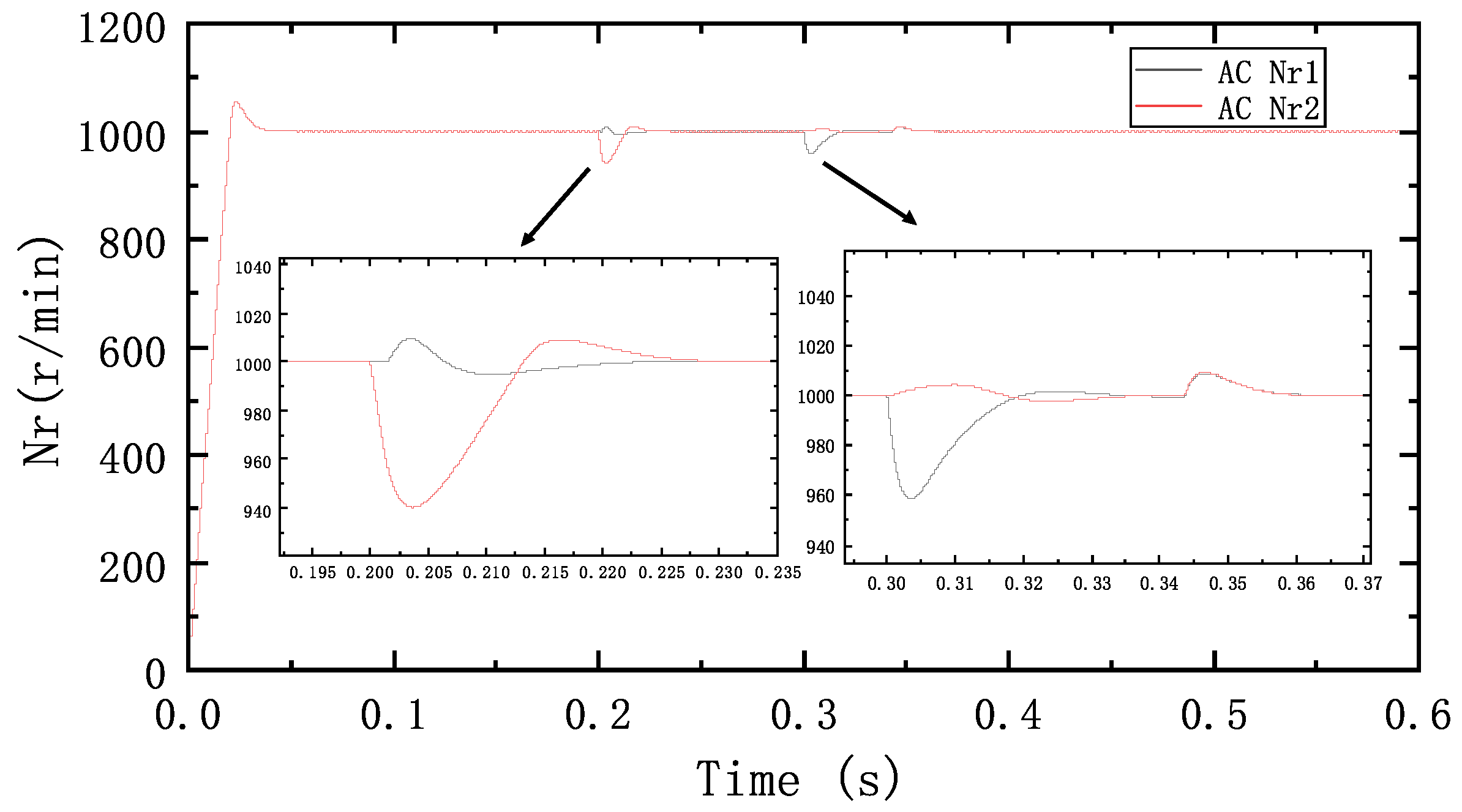
In the proposed adaptive control strategy, the d-axis current weighting coefficient in the cost function was set to ${\lambda }_d=0.001$. The load torques of the two motors were estimated by the load torque observer, and the load-difference threshold was set to $a=0.5$. The corresponding speed and three-phase current waveforms are shown in Figure 14 and Figure 15.

As shown in Figure 14, the overshoot of motor 1 under the proposed adaptive control is reduced compared with that under conventional predictive control. Moreover, as shown in Figure 15, the system exhibits improved stability and reduced noise, as reflected by the three-phase current waveform. Therefore, based on the proposed load torque observer, both the weighting coefficient K and the load-difference threshold a can be adjusted according to practical requirements in order to achieve an appropriate balance among dynamic response, stability, and computational cost.

4.4. Quantitative Performance Comparison

To provide a clearer comparative evaluation of the different control strategies, the main quantitative performance indices are summarized in

Table 4. Quantitative performance comparison under load disturbances.

Control Strategy	Max. Overshoot at 0.2 s	Max. Overshoot at 0.3 s	Current Waveform
Improved MSC	6.182%	8.023%	Good
AMC	6.216%	6.040%	Good
Conventional MPTC	4.611%	3.882%	Poor
Improved MPTC	5.137%	4.028%	Improved
Proposed adaptive control	5.193%	5.2082%	Improved

. The selected indices include the speed overshoot under the load disturbance at 0.2 s, the speed overshoot or speed fluctuation under the load disturbance at 0.3 s, and the current waveform quality. These indices directly reflect the transient speed response and current regulation performance of the dual-motor system under load imbalance.

Harmonic components have been recognized as an important factor in the performance evaluation of power electronic systems. For example, Niu et al. investigated the optimal resonant condition for maximum output power in tightly coupled wireless power transfer systems by considering harmonic components [39]. Although the application scenario of that study is different from the single-inverter dual-PMSM drive system considered in this paper, it shows that harmonic effects should not be ignored when evaluating power electronic systems. Therefore, in addition to the time-domain current waveform comparison, the total harmonic distortion (THD) of the three-phase currents is further calculated in this study.

To further quantitatively evaluate the influence of different control strategies on current harmonic distortion, the total harmonic distortion (THD) of the three-phase currents was calculated. The THD index is used to evaluate the harmonic content of the phase current and is defined as

$${\mathrm{THD}}_i={\displaystyle \frac{\sqrt{I_2^2+I_3^2+\dots +I_n^2}}{I_1}}\times 100\%,$$

(93)

where $I_1$ is the fundamental current component, and $I_2,I_3,\dots ,I_n$ are the harmonic components. In this study, the THD values of the three-phase currents of both motors were calculated over the whole simulation interval from 0 to $0.6\mathrm{s}$. For each motor, the THD values of the three-phase currents were first calculated and then averaged. The average THD of the two motors was further used as the overall current harmonic distortion index. The THD comparison results under different control strategies are summarized in

Table 5. THD comparison of three-phase currents under different control strategies.

Control Strategy	Average THD of Motor 1 (%)	Average THD of Motor 2 (%)	Average Current THD (%)
Improved MSC	1.2888	1.1145	1.2017
AMC	1.1319	0.9576	1.0448
Conventional MPTC	33.5983	34.7367	34.1675
Improved MPTC	2.9445	3.0661	3.0053
Proposed adaptive control	4.8761	3.3601	4.1181

.

As shown in Table 5, the conventional MPTC method has the highest average current THD, reaching $34.1675\%$, which indicates that its current waveform contains significant harmonic distortion. This result is consistent with the time-domain current waveform shown in the simulation results. By contrast, the improved MPTC and the proposed adaptive control strategy significantly reduce the current THD. In particular, the average current THD of the proposed adaptive control strategy is reduced to $4.1181\%$, which verifies that the introduced current regulation term and adaptive control mechanism can effectively improve the current waveform quality compared with conventional MPTC.

It can also be observed that the Improved MSC and AMC methods exhibit lower current THD values. However, according to the speed-response comparison in Table 4, these methods show larger speed deviations under load disturbances. Therefore, the proposed adaptive control strategy does not simply pursue the lowest current THD, but achieves a better compromise between transient speed response and current waveform quality under load imbalance.

These THD results provide a quantitative harmonic evaluation of the current waveform improvement. Therefore, the improvement in current quality is not only observed from the time-domain current waveforms, but also verified by the reduction of current harmonic distortion compared with conventional MPTC.

4.5. Robustness Verification Under Time-Varying Load Disturbances

The preceding simulations mainly verify the effectiveness of the proposed adaptive control strategy under step load disturbances. However, in practical dual-motor drive systems, the load torque may vary continuously or irregularly rather than only in a stepwise manner. Therefore, to further examine the robustness of the sliding mode observer and the validity of the assumption that the load torque remains approximately constant within one control period, additional simulations were carried out under three types of time-varying load disturbances, namely ramp load disturbance, periodic load disturbance, and stochastic load disturbance.

In these tests, the controller parameters were kept the same as those listed in Table 3. The reference speed was still set to $1000\mathrm{rpm}$, and both motors initially operated under a load torque of $12\mathrm{N}·\mathrm{m}$. The three time-varying load disturbances were applied to the two motors to evaluate both the tracking capability of the load-torque observer and the dynamic response of the proposed adaptive controller.

For the ramp-load disturbance case, the final load torque of each motor was still set to $22\mathrm{N}·\mathrm{m}$, corresponding to an additional load of $10\mathrm{N}·\mathrm{m}$. Different from the step-load case, the sudden load increments were replaced by ramp load variations. Specifically, the load torque of motor 2 started to increase linearly at $0.2\mathrm{s}$ and reached $22\mathrm{N}·\mathrm{m}$ at $0.5\mathrm{s}$, while the load torque of motor 1 started to increase linearly at $0.3\mathrm{s}$ and reached $22\mathrm{N}·\mathrm{m}$ at $0.5\mathrm{s}$. Therefore, the ramp slope of motor 2 was set to $33.33\mathrm{N}·\mathrm{m}/\mathrm{s}$, and the ramp slope of motor 1 was set to $50\mathrm{N}·\mathrm{m}/\mathrm{s}$. The ramp load torques of the two motors are defined as

$$T_{L1}\left(t\right)=\left\{\begin{array}{cc}12,\hfill & t<0.3,\hfill \\ 12+50(t-0.3),\hfill & 0.3\le t<0.5,\hfill \\ 22,\hfill & t\ge 0.5,\hfill \end{array}\right.$$

(94)

$$T_{L2}\left(t\right)=\left\{\begin{array}{cc}12,\hfill & t<0.2,\hfill \\ 12+{\displaystyle \frac{100}{3}}(t-0.2),\hfill & 0.2\le t<0.5,\hfill \\ 22,\hfill & t\ge 0.5.\hfill \end{array}\right.$$

(95)

For the periodic-load disturbance case, the load torque was designed to vary periodically between $12\mathrm{N}·\mathrm{m}$ and $22\mathrm{N}·\mathrm{m}$, so that its disturbance magnitude remained consistent with the step-load case. The disturbance frequency was set to $5\mathrm{Hz}$. The load torque of motor 2 started to vary periodically at $0.2\mathrm{s}$, while that of motor 1 started to vary periodically at $0.3\mathrm{s}$. The periodic load torques are expressed as

$$T_{L1}\left(t\right)=\left\{\begin{array}{cc}12,\hfill & t<0.3,\hfill \\ 12+5\left[1-cos\left(2\pi ·5(t-0.3)\right)\right],\hfill & t\ge 0.3,\hfill \end{array}\right.$$

(96)

$$T_{L2}\left(t\right)=\left\{\begin{array}{cc}12,\hfill & t<0.2,\hfill \\ 12+5\left[1-cos\left(2\pi ·5(t-0.2)\right)\right],\hfill & t\ge 0.2.\hfill \end{array}\right.$$

(97)

For the stochastic-load disturbance case, the load torque was designed as a bounded random fluctuation around the post-disturbance load level. To maintain consistency with the step-load case while avoiding unrealistically large random jumps, the nominal post-disturbance load torque was set to $22\mathrm{N}·\mathrm{m}$, and a bounded stochastic component was added after the load-change instant. The stochastic load torques are defined as

$$T_{L1}\left(t\right)=\left\{\begin{array}{cc}12,\hfill & t<0.3,\hfill \\ 22+n_1\left(t\right),\hfill & t\ge 0.3,\hfill \end{array}\right.$$

(98)

$$T_{L2}\left(t\right)=\left\{\begin{array}{cc}12,\hfill & t<0.2,\hfill \\ 22+n_2\left(t\right),\hfill & t\ge 0.2,\hfill \end{array}\right.$$

(99)

where $n_1\left(t\right)$ and $n_2\left(t\right)$ are bounded random disturbances satisfying

$$|n_1\left(t\right)|\le 1\mathrm{N}·\mathrm{m},|n_2\left(t\right)|\le 1\mathrm{N}·\mathrm{m}.$$

(100)

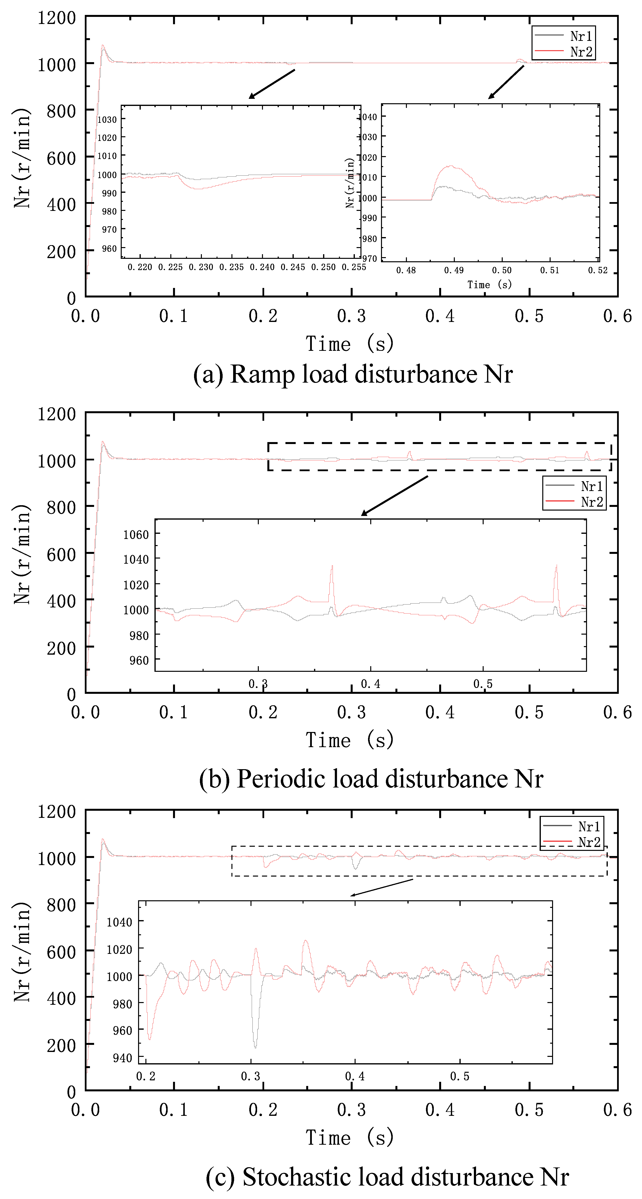
Figure 16 shows the speed responses of the two motors under the three types of time-varying load disturbances. As shown in Figure 16a, under the ramp-load disturbance, the speeds of the two motors remain close to the reference speed during the gradual load increase, and no severe speed oscillation occurs. Figure 16b shows that, under the periodic-load disturbance, the motor speeds exhibit only small periodic fluctuations around the reference speed. Figure 16c further shows that, although the stochastic-load disturbance introduces more irregular speed fluctuations, the proposed adaptive controller can still suppress large speed deviations and maintain stable operation of the dual-motor system.

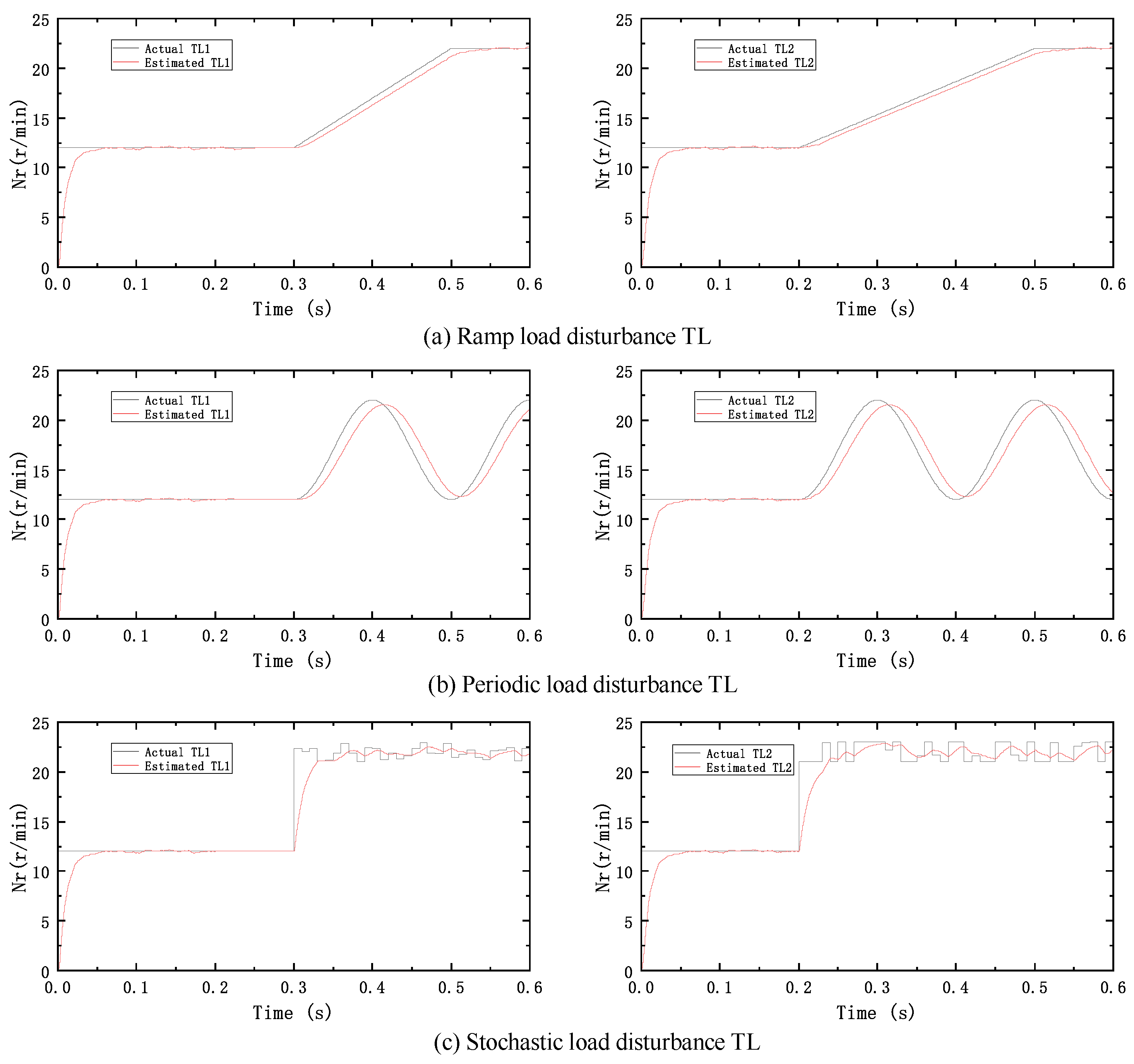
To further evaluate the load-torque estimation performance of the sliding mode observer, Figure 17 compares the actual and estimated load torques of motor 1 and motor 2 under the same three time-varying load disturbances. In the ramp-load case, the estimated load torques of both motors follow the continuously increasing actual load torques, with only a slight delay caused by the low-pass filtering process. In the periodic-load case, the observer can track the main periodic variation of the actual load torque. In the stochastic-load case, although small estimation fluctuations appear because of the random load component, the estimated load torque remains consistent with the overall variation trend of the actual load torque.

Since the proposed adaptive controller uses the estimated load-torque difference between the two motors as the control-mode switching variable, the accurate estimation of both motor loads is important for reliable mode selection. The results in Figure 17 indicate that the estimated load torques of both motors can follow the imposed ramp, periodic, and stochastic load variations. Therefore, the estimated load-torque difference can still reflect the actual load imbalance under non-step load disturbances, which supports the effectiveness of the adaptive switching mechanism.

These additional simulation results verify that the assumption of constant load torque within one control period is reasonable when the sampling period is sufficiently small and the load variation rate is bounded. This assumption does not require the load torque to remain constant during the whole operation process. Instead, it means that the load torque can be regarded as approximately piecewise constant within each short control period. Under this condition, the sliding mode observer can update the estimated load torque in real time and provide an effective load-imbalance indicator for the adaptive control strategy.

Therefore, the proposed sliding mode observer and adaptive controller are not only effective under step load disturbances, but also maintain acceptable robustness under ramp, periodic, and stochastic load disturbances. Nevertheless, under highly irregular stochastic loads, the estimation fluctuation may increase because of random load variation and low-pass filtering delay. This indicates that the observer gain, boundary-layer thickness, and filter cutoff frequency should be jointly selected according to the expected load variation rate and measurement noise level in practical applications.

4.6. Parameter Sweep of the d-Axis Current Weighting Coefficient

The d-axis current weighting coefficient ${\lambda }_d$ in the improved MPTC cost function directly affects the trade-off between transient speed response and current waveform quality. In the preceding simulations, ${\lambda }_d=0.002$ was selected as the nominal value. To further examine the influence of this parameter and improve the reproducibility of the parameter selection, a wider parameter sweep was carried out by varying ${\lambda }_d$ while keeping all other controller parameters unchanged.

In the parameter sweep, ${\lambda }_d$ was selected as $0.001$, $0.002$, $0.003$, and $0.004$, respectively. A smaller value of ${\lambda }_d$ gives higher priority to torque tracking and speed response, whereas a larger value of ${\lambda }_d$ increases the penalty on the predicted d-axis current and thus strengthens the current waveform regulation effect. The simulations were performed under the same load-disturbance condition as that used in Section 4.3, namely both motors initially operated under $12\mathrm{N}·\mathrm{m}$ load torque, an additional $10\mathrm{N}·\mathrm{m}$ load was applied to motor 2 at $0.2\mathrm{s}$, and an additional $10\mathrm{N}·\mathrm{m}$ load was applied to motor 1 at $0.3\mathrm{s}$.

The parameter sweep results are summarized in

Table 6. Parameter sweep results of the d-axis current weighting coefficient.

${\mathit{\lambda }}_{\mathit{d}}$	Max. Speed Deviation at 0.2 s (%)	Max. Speed Deviation at 0.3 s (%)	Average Current THD (%)
0.001	5.1936	5.2082	4.1118
0.002	5.2421	5.4237	3.0597
0.003	5.2863	5.5384	2.4659
0.004	5.3268	5.6212	2.1840

. The selected performance indices include the maximum speed deviation after the load disturbance at $0.2\mathrm{s}$, the maximum speed deviation after the load disturbance at $0.3\mathrm{s}$, and the average current THD. The maximum speed deviation is used to evaluate the transient speed response, while the average current THD is used to evaluate the three-phase current waveform quality. In this study, the current THD was calculated over the whole simulation interval from 0 to $0.6\mathrm{s}$, so that both the transient process and the post-disturbance current waveform quality were considered. For the dual-motor system, the THD values of the three-phase currents of both motors were first calculated, and their average value was used as the current-quality index.

As shown in Table 6, increasing ${\lambda }_d$ reduces the average current THD, indicating that the d-axis current suppression term is beneficial for improving the three-phase current waveform quality. Specifically, when ${\lambda }_d$ increases from $0.001$ to $0.002$, the average current THD decreases from $4.1118\%$ to $3.0597\%$. This result confirms that the introduced d-axis current weighting term can effectively improve current quality.

However, the speed response is slightly affected when ${\lambda }_d$ increases. The maximum speed deviation at $0.2\mathrm{s}$ increases from $5.1936\%$ to $5.2421\%$, and the maximum speed deviation at $0.3\mathrm{s}$ increases from $5.2082\%$ to $5.4237\%$ when ${\lambda }_d$ changes from $0.001$ to $0.002$. When ${\lambda }_d$ is further increased to $0.003$ and $0.004$, the current THD continues to decrease, but the speed deviation also becomes larger. This indicates that an excessively large ${\lambda }_d$ gives too much priority to current waveform regulation and may weaken the torque tracking priority, thereby slightly deteriorating the transient speed response.

Therefore, ${\lambda }_d$ should not be selected only by minimizing the current THD. Instead, it should be determined by balancing speed response and current waveform quality. In this study, ${\lambda }_d=0.002$ provides a suitable compromise: compared with ${\lambda }_d=0.001$, it significantly reduces the average current THD, while the increase in speed deviation remains limited. Thus, ${\lambda }_d=0.002$ was adopted in the subsequent comparative simulations.

4.7. Discussion on Validation Scope

The simulation results presented above verify the basic effectiveness of the proposed adaptive control strategy under load-step conditions. The results show that the proposed method can reduce speed oscillation and improve the three-phase current waveform compared with conventional control strategies. However, the present validation is still based on MATLAB/Simulink simulations under a nominal motor model.

In practical applications, parameter mismatch, measurement noise, inverter nonlinearity, sampling delay, and time-varying load disturbances may further affect the control performance. Although the revised observer design has considered bounded parameter uncertainty and modeling errors in the robustness analysis, additional simulation and experimental verification under non-ideal conditions are still necessary to further evaluate the practical robustness of the proposed method. Therefore, future work will focus on robustness tests under parameter mismatch, noisy feedback signals, time-varying load disturbances, and hardware-in-the-loop or experimental platform validation.

Although the simulation results verify the effectiveness of the proposed adaptive control strategy under step load disturbances, time-varying load disturbances, and different values of the d-axis current weighting coefficient, the present validation is still based on MATLAB/Simulink simulations. Hardware-in-the-loop tests and experimental validation have not yet been conducted in this study because a complete single-inverter dual-PMSM experimental platform and the corresponding real-time control hardware are not currently available.

Therefore, the practical implementation performance of the proposed method still requires further verification. In real drive systems, inverter nonlinearity, dead-time effect, sampling delay, sensor noise, parameter mismatch, thermal variation, and mechanical coupling characteristics may affect the observer accuracy and control performance. These non-ideal factors should be further considered in future HIL and experimental studies.

Future work will focus on constructing a real-time control platform for the single-inverter dual-PMSM system. The proposed sliding mode torque observer, adaptive switching mechanism, and improved MPTC strategy will be implemented on a real-time controller to evaluate their performance under realistic industrial load profiles. This will further verify the practical feasibility and robustness of the proposed control scheme.

5. Conclusions

This paper proposed a load-imbalance-aware hybrid control strategy for a single-inverter dual-PMSM system under load disturbance. In the proposed method, the load-torque difference estimated by the sliding mode observer is used as a physical indicator of the operating condition of the strongly coupled dual-motor system. According to the estimated load imbalance, the controller adaptively allocates the control mode between vector control and finite-set model predictive torque control. Therefore, the proposed strategy reduces the dependence on permanently fixed master–slave role assignment under balanced or weakly unbalanced load conditions, while improving disturbance rejection under strongly unbalanced load conditions.

Compared with average-model-based control, the proposed strategy reduces speed overshoot under load disturbance. Compared with conventional predictive torque control, the proposed method improves the three-phase current waveform quality while maintaining favorable dynamic response. In addition, because predictive torque control is activated only when the estimated load-torque difference becomes significant, unnecessary full-time predictive optimization can be avoided. Therefore, the average number of predictive evaluations can be reduced compared with a control scheme based entirely on predictive torque control.

The simulation results indicate that the proposed strategy can achieve smooth control−mode switching under varying load torque conditions and can provide improved speed tracking and stability for the single−inverter dual−PMSM system. Furthermore, the results show that the load-difference threshold a and the weighting factor ${\lambda }_d$ affect the trade−off among dynamic response, current waveform quality, and computational effort. A smaller value of a allows earlier activation of predictive torque control but may increase the average predictive evaluation burden. A larger value of ${\lambda }_d$ suppresses d-axis current fluctuation more effectively and improves current waveform quality, but it may also affect the speed transient response. By contrast, a smaller value of ${\lambda }_d$ helps maintain faster speed convergence but weakens the d-axis current suppression capability.

The present study is mainly based on MATLAB/Simulink simulation under load−disturbance conditions. Although the simulation results demonstrate the basic effectiveness of the proposed adaptive control strategy, further verification under parameter mismatch, measurement noise, inverter nonlinearity, sampling delay, and time−varying load disturbances is still required. In future work, hardware−in−the−loop tests and experimental validation will be carried out to further evaluate the practical robustness and real−time implementation performance of the proposed method.