Expert-Transformer with Prototype-Aware Contrastive Learning for Semi-Supervised Time-Series Classification

Abstract

Semi-supervised time-series classification (TSC) faces challenges in handling intra-class variability and distribution shifts, which limit the effectiveness of standard contrastive learning methods. To address these limitations, we propose the Expert-Transformer with Prototype-Aware Contrastive Learning (ExT-PACL), a novel framework that integrates an uncertainty-guided Mixture-of-Experts (MoE) module within a Transformer encoder to dynamically capture diverse temporal patterns. An expert balancing strategy ensures all experts contribute meaningfully, preventing collapse and enhancing representation robustness. In addition, a prototype-aware contrastive learning loss guides both labeled and high-confidence unlabeled samples toward class prototypes, improving discriminative power and reducing reliance on large negative sample sets. Extensive experiments on multiple benchmark datasets demonstrate that ExT-PACL achieves superior generalization and state-of-the-art performance.

1. Introduction

Time-series classification (TSC) is a fundamental task in data mining and machine learning, with extensive applications in healthcare (e.g., ECG/EEG interpretation) [1], industrial systems (sensor anomaly detection) [2], finance (market regime identification) [3], and human activity recognition [4]. The advances of deep learning have naturally influenced TSC, yielding impressive performance [5,6,7]. Nevertheless, in many practical settings, obtaining labeled data is highly costly and labor-intensive, which significantly limits the feasibility of fully supervised approaches.

Semi-Supervised Learning (SSL) provides an effective strategy by combining a limited amount of labeled data with a large pool of unlabeled samples. Within SSL approaches, contrastive learning has gained considerable attention. Its main idea is to construct a consistent representation space in which similar (positive) sample pairs are drawn together, while dissimilar (negative) pairs are separated. Techniques such as Contrastive Predictive Coding (CPC) and SimCLR have been successfully extended to time-series data [8,9]. For example, Eldele et al. [10] introduced a robust baseline for TSC by employing a temporal contrastive loss combined with carefully designed data augmentations.

Semi-supervised contrastive learning for TSC, despite its effectiveness, remains constrained by the inability to handle intra-class diversity and distribution shifts. Standard models treat all temporal patterns uniformly, which limits their capacity to extract discriminative features across varying samples of the same class. This limitation motivates the integration of a Mixture-of-Experts (MoE) system: by assigning samples to specialized experts based on uncertainty, the model can dynamically capture diverse temporal characteristics, ensuring that rare or non-dominant patterns receive appropriate attention. Furthermore, to avoid imbalanced expert utilization and potential collapse, a balancing strategy is employed, guaranteeing that each expert contributes meaningfully to representation learning. In this way, the MoE framework becomes essential for semi-supervised contrastive learning, directly addressing the challenges of overfitting, non-uniform intra-class patterns, and insufficiently discriminative representations, thereby linking the model design to the fundamental limitations of existing approaches.

This paper presents a novel architecture, Expert-Transformer with Prototype-Aware Contrastive Learning (ExT-PACL), designed to address the significant challenges in semi-supervised time-series classification. Traditional models often struggle to generalize across diverse temporal patterns within a single class due to the lack of specialized mechanisms. To address this, we propose the integration of an uncertainty-guided Mixture-of-Experts (MoE) system within the Transformer encoder. Each expert in this framework is a neural network tailored to handle specific types of temporal data, such as periodic signals, transient spikes, or noisy segments. By incorporating uncertainty estimation, the gating mechanism dynamically routes each input token or sequence to the most relevant combination of experts, enabling the model to adaptively specialize on diverse patterns. This approach enhances the model’s ability to generalize across unseen temporal variations and builds domain-specific expertise internally, addressing one of the key challenges in TSC.

Furthermore, the introduction of an expert balancing strategy ensures that the MoE system remains robust, preventing expert collapse and ensuring that each expert contributes meaningfully to the learning process. This expert balancing strategy further improves the model’s adaptability to various temporal patterns, while maintaining a cohesive representation of the underlying data structure. Overall, our contributions lie in the synergistic combination of an uncertainty-guided MoE system, a prototype-aware contrastive loss, and an expert balancing strategy, providing a comprehensive solution that addresses the core challenges in semi-supervised time-series classification and sets a new direction for future research in this area.

Finally, to enhance the discriminative power of the learned representations and reduce reliance on large numbers of negative samples, we introduce a prototype-aware contrastive learning loss. In our semi-supervised framework, we iteratively compute class prototypes from the data feature representations and the classification outcomes. These prototypes serve as anchors in the contrastive learning process, where the loss function actively pulls both labeled and high-confidence unlabeled samples toward their respective class prototypes while repelling them from others. This mechanism injects essential categorical semantics into the learning process, enabling the model to distinguish between classes more effectively. Combined with the MoE system, this prototype-aware loss not only improves the model’s ability to generalize across diverse patterns but also aligns the learned features with the final classification task, thus overcoming the challenges of poor intra-class discrimination and overfitting.

Our main contributions are summarized as follows:

1.

We integrate an uncertainty-guided Mixture-of-Experts (MoE) with the Transformer encoder, enabling dynamic routing of input sequences to specialized experts and improving generalization across diverse temporal patterns.

2.

An expert balancing strategy, which prevents expert collapse and ensures meaningful contribution from all experts, is designed to enhance robustness and adaptability.

3.

We introduce a prototype-aware contrastive learning loss, which iteratively computes class prototypes and guides both labeled and high-confidence unlabeled samples, embedding categorical semantics to strengthen discriminative feature learning.

4.

We conduct extensive experiments on public benchmark datasets. The results demonstrate that ExT-PACL consistently outperforms state-of-the-art SSL methods, particularly in extreme low-label scenarios, while also being more computationally efficient than standard contrastive baselines.

2. Related Work

2.1. Semi-Supervised Time-Series Classification

Self-supervised learning (SSL) seeks to mitigate the reliance on large labeled datasets by pre-training models on tasks designed for unlabeled data. The central idea is to learn a representation space where embeddings remain invariant under semantically meaningful data augmentations, thereby capturing essential temporal features. For instance, the SelfMatch framework employs a form of self-distillation, where a “weakly augmented” version of a time-series guides the learning process of a “strongly augmented” version [11]. This flow of knowledge from the more stable view to the perturbed one encourages the model to generate consistent embeddings, thus directly fostering invariance to these augmentations.

A key focus in semi-supervised time-series classification (TSC) is the development of innovative architectures that effectively utilize the structure of unlabeled data. Graph-based approaches have demonstrated considerable potential. For instance, the ITS2Graph framework redefines TSC as a node classification task within a graph, where nodes represent time-series samples derived from their latent features [12]. The framework further employs graph generative adversarial learning to generate samples for minority classes, effectively addressing the pervasive challenge of class imbalance—an issue common in semi-supervised settings with limited and potentially biased labeled data.

Additionally, ensemble methods are gaining traction for enhancing the reliability of pseudo-labeling, a critical aspect of many SSL algorithms. The CE-SFDA framework uses a classifier ensemble to produce more accurate pseudo-labels for the target domain, complemented by a memory-aware knowledge distillation technique that captures both global and local data structures [13]. This ensemble strategy reduces the propagation of errors from noisy pseudo-labels, which is a frequent issue in iterative SSL methods. Another emerging trend is the conversion of time-series data into other modalities to leverage the power of architectures from diverse fields. The TS-BCT framework, for example, learns discriminative time-series representations through temporal-specific augmentations and bidirectional consistency regularization [14]. It aims to establish a feature space with well-defined class boundaries, even in the absence of abundant labeled data. By incorporating pseudo-labels from both augmented views, TS-BCT creates class-relevant contrastive patterns, reinforcing bidirectional consistency and aiding the model in learning a more distinct and separable feature space.

2.2. Contrastive Representation Learning for Time-Series

A key application of contrastive learning in time-series classification (TSC) is the extraction of transferable representations from unlabeled data. The success of this approach hinges on designing effective data augmentation strategies and contrastive objectives that capture robust temporal features.

The TS-TCC framework introduces a novel contrastive learning method, applying both weak (e.g., jittering and scaling) and strong (e.g., permutation and jitter) augmentations to raw time-series data [15]. It incorporates a unique temporal contrastive module that conducts a extra prediction task, encouraging the model to learn resilient temporal representations. This is further strengthened by a contextual contrastive module, which maximizes the similarity between contexts derived from different augmentations of the same sample, while minimizing the similarity between contexts from distinct samples.

The iBACon method addresses the challenge of predicting rare, high-difficulty events (e.g., sudden spikes in power demand) by introducing an Imbalance-Aware Contrastive Learning framework [16]. This approach quantifies sample difficulty using an Input–Output Difference (IOD) metric and groups samples with similar difficulty levels within the feature space. Additionally, DSDCLNet provides a solution for Multivariate Time-Series Classification, featuring a hierarchical dual-level design, which is particularly effective in semi-supervised settings where labeled data is limited [17]. The model’s innovation lies in its structured approach to learning representations at multiple granularities, enhancing its adaptability to varying data complexities.

3. Methodology

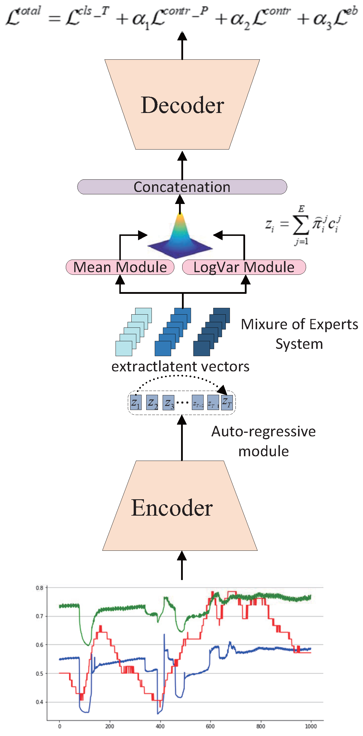
In this section, we will introduce the detailed schematic of the ExT-PACL framework, which is shown in Figure 1. The input time-series is first transformed into a sequence of embeddings. This sequence is processed by a stack of MoE-Transformer encoder layers. The output contextualized embeddings are used for two purposes: (1) to compute a standard classification loss via a linear projector for labeled data, and (2) to be aggregated into the prototype predicted vectors. These vectors are then used to compute the proposed prototype-aware contrastive learning loss and expert balancing loss, which supervises the learning of unlabeled data.

3.1. Problem Formulation

Let $\mathcal{X}={\mathcal{X}}_L\cup {\mathcal{X}}_U$ denote the entire dataset, where ${\mathcal{X}}_L=\{(x_1,y_1),\dots ,(x_M,y_M)\}$ is the labeled dataset and ${\mathcal{X}}_U=\{x_{M+1},\dots ,x_N\}$ is the unlabeled dataset, $M\ll N$. For the labeled dataset, the i-th time sequence $x_i\in {\mathbb{R}}^{T\times C}$ with T time steps has C channels. $y_i$ is the corresponding class label. The goal of STSC is to learn a mapping function $f_{\theta }:{\mathbb{R}}^{T\times C}\to {\mathbb{R}}^K$ by leveraging ${\mathcal{X}}_L$ and ${\mathcal{X}}_U$. K is the number of classes.

3.2. MoE-Enhanced Expert-Transformer

In STSC, we should learn comprehensive representations from unlabeled data to improve the generalization performance of the model. Considering that input data usually have the time-dependent and non-stationary characteristic, a novel Mixture-of-Experts model is designed to combine information from different experts.

First, we adopt a convolutional-based encoder $f_{en}$ and a Transformer-based auto-regressive module $f_{ar}$ to extract features from raw data first. Specifically, an input series $x_i$ is projected into a sequence of vectors, $h_i=f_{enc}\left(x_i\right),h_i\in {\mathbb{R}}^{T\times D}$. T is the time step. D denotes the feature dimension. As in the paper [10], features from different time steps are summarized into a context vector $c_i\in {\mathbb{R}}^D$

$$\begin{array}{c}\hfill c_i=f_{ar}\left(h_i\right)\end{array}$$

(1)

However, a standard Transformer-based auto-regressive module might struggle to handle inherent variability and uncertainty of unlabeled data and result in poor generalization, since the model must infer patterns in the absence of explicit ground-truth annotations. By employing multiple “experts” (specialized sub-models), each adept at processing specific data types (e.g., temporal patterns), the system can internally develop domain expertise. Specifically, we reinterpret the expert routing variable e as a latent random variable conditioned on the contextual representation $c_i$, where the router models a posterior distribution for learning the latent temporal dynamics of sample $x_i$

$$\begin{array}{c}\hfill q_{\theta }(e\mid c_i)=\mathrm{Softmax}(W_e{c}_i+b_e)\end{array}$$

(2)

In this way, the expert assignment can be viewed as categorical distribution, $e_i\sim \mathrm{Categorical}\left(q_{\theta }(e\mid c_i)\right)$.

Hence, we propose to integrate an uncertainty-based expert system into semi-supervised classification. Specifically, the context vector is viewed as the input of the expert system

$$\begin{array}{c}\hfill c_i^e=f_{ar}^e\left(h_i\right),e=1,\dots ,E\end{array}$$

(3)

In the experiment, the number of experts E is set to 4. Then, the router score of a specific expert is formulated as follows:

$$\begin{array}{c}\hfill s_i^e=W^e{c}_i^e+b^e\end{array}$$

(4)

$(W^e,b^e)$ is a learnable parameter for the e-th expert. By the way, we can learn the expert weight based on the router scores of all experts

$$\begin{array}{c}\hfill {\pi }_i^e={\displaystyle \frac{exp\left(s_i^e\right)}{{\sum }_{j=1}^{E}exp\left(s_i^j\right)}}\end{array}$$

(5)

The aggregated output obtained through the expert system is defined as

$$\begin{array}{c}\hfill z_i={\displaystyle \sum _{j=1}^E}{\pi }_i^j{c}_i^j\end{array}$$

(6)

To alleviate the distribution shift problem caused by the uncertainty expert decision, we propose to quantify the expert decision distribution by the uncertainty estimation. First we calculate the mean vector and variance vector of expert weights

$$\begin{array}{c}\hfill {\mu }_i={\displaystyle \frac{1}{E}}{\displaystyle \sum _e^E}{\pi }_i^e,{\sigma }_i^e={\pi }_i^e(1-{\pi }_i^e)\end{array}$$

(7)

Because ${\pi }_i^e$ is the softmax output and follows a multinomial distribution, the variance vector of each expert ${\sigma }_i^e$ is expressed in the form of $p(1-p)$. Based on the definition, the covariance vector is represented as

$$\begin{array}{c}\hfill {\mathsf{\Sigma }}_i=diag({\sigma }_i^{1^2},{\sigma }_i^{2^2},\dots ,{\sigma }_i^{E^2})\end{array}$$

(8)

where non-diagonal elements are 0. Correspondingly, the inverse covariance is formulated as a zero-padded diagonal matrix

$$\begin{array}{c}\hfill {\mathsf{\Sigma }}_i^{-1}=diag({\displaystyle \frac{1}{{\sigma }_i^{1^2}}},{\displaystyle \frac{1}{{\sigma }_i^{2^2}}},\dots ,{\displaystyle \frac{1}{{\sigma }_i^{E^2}}})\end{array}$$

(9)

This design allows the model to learn specialized experts and to make soft, uncertainty-aware decisions.

After that, we compute the final expert weight through the uncertainty-aware fusion mechanism. The core key is apply the gated correction formula weighted by Mahalanobis distance to reduce the weight of experts with high uncertainty and increase the weight of those with low uncertainty

$${\stackrel{⌢}{\pi }}_i^e=\frac{{\pi }_i^e•\exp (-\frac{1}{2}({({\pi }_i^e-{\mu }_i)}^T{\mathsf{\Sigma }}_i^{-1}({\pi }_i^e-{\mu }_i)))}{{\sum }_{j=1}^E{\pi }_i^j•\exp (-\frac{1}{2}({({\pi }_i^j-{\mu }_i)}^T{\mathsf{\Sigma }}_i^{-1}({\pi }_i^j-{\mu }_i))}$$

(10)

Because ${\mathsf{\Sigma }}_i^{-1}$ is the diagonal matrix, the Mahalanobis distance calculation can be simplified as

$${\stackrel{⌢}{\pi }}_i^e=\frac{{\pi }_i^e•\exp (-\frac{{({\pi }_i^e-{\mu }_i)}^2}{2{{\sigma }_i^e}^2})}{{\sum }_{j=1}^E{\pi }_i^j•\exp (-\frac{({\pi }_i^j-{\mu }_i{)}^2}{2{{\sigma }_i^j}^2})}$$

(11)

Thus, the uncertainty-aware expert weight still follows ${\sum }_{j=1}^E{\stackrel{⌢}{\pi }}_i^j$ = 1. Meanwhile, the greater the deviation of the initial expert weight ${\pi }_i^e$ from the mean, and the smaller its own variance (the lower the uncertainty), the higher its final weight will be.

In summary, instead of the original Transformer-based auto-regressive module, we propose to employ the MoE-Enhanced Transformer module to capture more generalized features

$$\begin{array}{c}\hfill z_i={\displaystyle \sum _{j=1}^E}{\stackrel{⌢}{\pi }}_i^j{c}_i^j\end{array}$$

(12)

3.3. Balanced Expert Training and Prototype-Guided Representation Learning

Recent developments in learning-based optimization (LBO) and physics-informed learning (PIL) highlight the integration of data-driven models with domain-specific knowledge for improved generalization and optimization performance [18,19]. Inspired by these studies, our approach leverages multiple specialized experts in a Transformer encoder and prototype-aware contrastive loss to adaptively capture diverse temporal patterns while embedding structural information inherent to the time-series data.

To make experts have more “specialization” and avoid the situation where routers in the early stage of training compress all the samples onto one or a few experts, the posterior expert distribution $q_{\theta }\left(e\right|x)$ should be peak or low entropy. In this way, all experts are needed for each sample equally. A corresponding expert balancing loss is designed

$$\begin{array}{c}\hfill {\mathcal{L}}^{\rceil \lfloor }=\mathbb{E}\left[KL\right(q_{\theta }\left(e\right|x)\left|\right|p\left(e\right)\left)\right]\end{array}$$

(13)

Thus, the posterior expert distribution $q_{\theta }\left(e\right|x)$ is enforced to be consistent with the prior expert distribution $p\left(e\right)$, which is a uniform distribution. This variational regularization term constrains the posterior routing distribution toward a prior distribution $p\left(e\right)$, preventing posterior collapse and reducing the risk that a small subset of experts overfits noisy temporal patterns. This regularization encourages all experts to capture meaningful latent dynamics rather than memorizing local noise correlations.

As a regularization term based on the MoE model, this detailed KL divergence formula for each sample is

$$\begin{array}{c}\hfill KL(q_{\theta }\left(e\right|x)\left|\right|p\left(e\right))=\sum _j{\pi }_i^{j}log{\displaystyle \frac{{\pi }_i^j}{E}}\end{array}$$

(14)

where the prior expert distribution $p\left(e\right)$ is defined as $1/E$. $q_{{\theta }_i}\left(e\right|x)={\pi }_i^e$.

Moreover, for enhancing the specialization of the experts, we design a self-learning prototype-aware contrastive loss to make the expert outputs for the same type of input be closer to each other, while the expert outputs for different types of input are as far apart as possible. Conventional contrastive learning typically defines positives and negatives based on data augmentations or heuristics. For example, two augmented samples of the same unlabeled sample are a positive pair. While this learns robust features, the resulting feature space is not necessarily organized according to the class boundaries of the downstream task. The model learns invariance to augmentations but not necessarily discrimination between categorical concepts. This can lead to sub-optimal decision boundaries when fine-tuning with limited labels.

In this paper, we propose a novel self-learning contrastive learning loss to strengthen the collaborative effect among different experts. For a feature vector $z_i$, we define its positive sets based on its corresponding class prototype. The negative samples are feature vectors from other prototypes. In STSC, the prototype predicted vector of the i-th sample based on class prototypes is formulated as

$$\begin{array}{c}\hfill r_i={\displaystyle \sum _{k=1}^K}{\displaystyle \frac{e^{-dist(z_i,{\varphi }_k)}}{{\sum }_{j=1}^K{e}^{-dist(z_i,{\varphi }_j)}}}{\phi }_k\end{array}$$

(15)

where $dist$ denotes the euclidean metric, $\varphi$ represents class prototype vectors, and $\phi$ is the indicator vector.

In STSC, prototypes derived only from limited labeled data are often biased and fail to capture the intrinsic distribution of the unlabeled majority. Therefore, a self-learning mechanism is needed to iteratively refine prototype features by leveraging the structural information embedded in features of unlabeled data. By progressively updating prototypes according to temporal features, the model can better align latent representations with underlying class structures, thereby improving cluster compactness and inter-class separability, which ultimately enhances classification performance in STSC. This strategy takes the data feature representations z and the classification results v, $v_i=f_{pre}\left(z_i\right)$, as inputs to compute $\varphi$ and $\phi$ iteratively. The class prototype ${\varphi }^j$ is presented as

$$\begin{array}{c}\hfill {\varphi }^j={\varphi }^j-\eta {\displaystyle \frac{{\sum }_{i=1}^{n^j}({\varphi }^j-z_i)}{1+n^j}}\end{array}$$

(16)

where ${\varphi }^i,{\varphi }^j$ are the of i-th and j-th class prototype vectors. $n^j$ denotes the number of samples at j-th class. $\eta$ is the learning rate. At the beginning, ${\varphi }^i$ is defined as ${\displaystyle \frac{1}{K}}$. Thus, ${\phi }_i$ represents the indicator vector of the i-th class, which is defined as follows:

$$\begin{array}{c}\hfill {\phi }_j={\displaystyle \frac{{\phi }_j-\eta \frac{{\sum }_{i=1}^{n_j}({\phi }_j-v_i)}{1+n_j}}{{\sum }_{k=1}^K{\phi }_k-\eta \frac{{\sum }_{i=1}^{n_j}({\phi }_k-v_i)}{1+n_j}}}\end{array}$$

(17)

The initial value of ${\phi }_i$ is set to 1.

Since class prototypes are iteratively updated using both labeled and unlabeled samples, noisy pseudo-labels may introduce error propagation and cause semantic drift. To mitigate this issue, we adopt a reliability-aware prototype update mechanism. During the initial warm-up stage, class prototypes are initialized and updated only using labeled samples, which provides stable semantic anchors. After the warm-up stage, an unlabeled sample is allowed to participate in prototype updating only when its prediction confidence exceeds a predefined threshold and its predictions under weak and strong augmentations are consistent.

For an unlabeled sample $x_i$, we compute the posterior distributions from two augmented samples, ${\phi }_i^w,{\phi }_i^s$. The sample is selected for prototype updating only if

$$\begin{array}{c}\hfill \underset{k}{max}{\phi }_i^w\left(k\right)\ge \delta \end{array}$$

(18)

where $\delta$ is the confidence threshold. The selected unlabeled samples contribute to the prototype update with confidence-based weights and are added into the set $n_k$, while labeled samples remain the primary semantic anchors. In addition, the prototype update is performed with stop-gradient operation, so that unreliable pseudo-labels do not directly amplify gradient noise. This design reduces error propagation and stabilizes the semantic structure of the latent space.

Corresponding, the prototype-aware contrastive learning loss of the j-th sample is defined as follows:

$$\begin{array}{c}\hfill {\widehat{\ell }}_j^r=-log{\displaystyle \frac{exp(CS(r_j^1,r_j^2)/{\tau }_C)}{{\sum }_{k=1}^K[exp(CS(r_j^1,r_k^1)/{\tau }_C)+exp(CS(r_j^1,r_k^2)/{\tau }_C)]}},\end{array}$$

(19)

where ${\tau }_C$ is a temperature hyperparameter of contrastive learning. $CS$ represents the cosine similarity function.

All unlabeled data ${\mathcal{X}}_U$ are trained with the prototype-aware contrastive learning loss. The complete loss function is as follows:

$$\begin{array}{c}\hfill {\mathcal{L}}^{contr\_P}={\displaystyle \frac{1}{2(N-M)}}{\displaystyle \sum _{j=1}^{N-M}}{\ell }_j^p\end{array}$$

(20)

3.4. Training Losses

Finally, the overall loss function is defined as follows:

$$\begin{array}{c}\hfill {\mathcal{L}}^{total}={\mathcal{L}}^{cls\_T}+{\alpha }_1{\mathcal{L}}^{contr\_P}+{\alpha }_2{\mathcal{L}}^{contr}+{\alpha }_3{\mathcal{L}}^{eb}\end{array}$$

(21)

where ${\mathcal{L}}^{cls\_C}$ and ${\mathcal{L}}^{contr}$ are cross-entropy loss of labeled data and sample-wise contrastive learning loss of unlabeled data respectively. ${\alpha }_1$, ${\alpha }_2$, and ${\alpha }_3$ are the hyperparameters of the losses. The cross-entropy loss is designed to learn class information from labeled data

$$\begin{array}{c}\hfill {\mathcal{L}}^{cls\_T}={\displaystyle \frac{1}{M}}{\displaystyle \sum _{i=1}^M}H(y_i,v_i)\end{array}$$

(22)

where H is the cross-entropy.

Then, we utilize the sample-wise contrastive learning loss to maximize the similarity between $a_i^w$ and $a_i^s$ from two different augmented samples of unlabeled data, which are obtained by a contrastive head, $a_i^w=f_{ch}\left(z_i^w\right),a_i^s=f_{ch}\left(z_i^s\right)$. The features $(z_i^w,z_i^s)$ are extracted from augmented unlabeled data, the weak augmented samples $x_i^w$ and the strong augmented samples $x_i^s$. The sample-wise contrastive loss function of the i-th sample is given as follows:

$$\begin{array}{c}\hfill {\ell }_i^w=-log{\displaystyle \frac{exp\left(CS({\mathit{a}}_i^w,{\mathit{a}}_i^s)/{\tau }_I\right)}{{\sum }_{j=1}^{(N-M)}[exp\left(CS({\mathit{a}}_i^w,{\mathit{a}}_j^w)/{\tau }_I\right)+exp\left(CS({\mathit{a}}_i^w,{\mathit{a}}_j^s)/{\tau }_I\right)]}},\end{array}$$

(23)

$$\begin{array}{c}\hfill {\ell }_i^s=-log{\displaystyle \frac{exp\left(CS({\mathit{a}}_i^s,{\mathit{a}}_i^w)/{\tau }_I\right)}{{\sum }_{j=1}^{(N-M)}[exp\left(CS({\mathit{a}}_i^s,{\mathit{a}}_j^s)/{\tau }_I\right)+exp\left(CS({\mathit{a}}_i^s,{\mathit{a}}_j^w)/{\tau }_I\right)]}},\end{array}$$

(24)

where ${\tau }_I$ is the temperature hyperparameter of sample-wise contrastive learning loss. The whole sample-wise contrastive learning loss is defined as follows:

$$\begin{array}{c}\hfill {\mathcal{L}}^{contr}={\displaystyle \frac{1}{2N}}{\displaystyle \sum _{i=1}^N}({\ell }_i^w+{\ell }_i^s)\end{array}$$

(25)

4. Experiments

4.1. Datasets

We conduct experiments on three distinct datasets: two datasets from the UCR Repository (Wafer and PhalangesOutlinesCorrect), the Epileptic Seizure Recognition dataset [20], and a power grid dataset derived from real monitoring data collected from State Grid servers between March 2025 and May 2025.

4.2. Comparison Baselines

Comparison baselines include 3 classical SSL methods (e.g., SSL-ECG [21], CPC [8], SimCLR [9]), and 4 state-of-the-art contrastive methods (Mean-Teacher [22], DivideMix [23], SemiTime [24], FixMatch [25], TS-TCC [15], CA-TCC [10]).

4.3. Evaluation Metrics

Two evaluation metrics (accuracy and MF1-score) are employed on the experiment.

4.4. Implement Details

The overall framework of the proposed approach consists of three modules. First, an encoder is constructed to extract sequence features from raw data, which includes three convolutional blocks and a fully connected block. The size of three convolutional blocks is set to [32, 64, 64]. All convolutional blocks have a convolutional layer, BatchNorm layer, Relu function, and a MaxPooling layer, and the first convolutional block has an extra dropout layer. Subsequently, a MoE-Enhanced module is designed to develop domain expertise, which is composed of an auto-regressive layer, a router layer, and a feedforward layer. The auto-regressive layer is a Transformer network. The output dimension of the router layer is the number of experts. In our experiment, the number is set to 4. The feedforward layer is a fully connected layer and the size is set to 128. Finally, the learned category-specific feature representations are fed into a decoder to predict categories. The decoder is also a fully connected layer. We adopt the Adam optimizer for optimization, and the learning rate is set to 0.0003, and the batch size is set to 8.

4.5. Experimental Results

Semi-supervised classification results on two datasets—the Epileptic Seizure Recognition dataset and the UCR Repository datasets (Wafer and PhalangesOutlinesCorrect)—as presented in

Table 1. Performance comparison for semi-supervised time-series classification.

Datasets	Epilepsy		Wafer		POC
Methods	Accuracy	MF1-Score	Accuracy	MF1-Score	Accuracy	MF1-Score
1% of labeled data
Random Init	70.3 ± 2.1	66.2 ± 2.6	90.6 ± 1.6	58.1 ± 2.1	61.4 ± 0.0	38.3 ± 0.0
Supervised	76.1 ± 0.7	74.8 ± 0.4	91.9 ± 1.3	67.6 ± 9.2	62.0 ± 0.8	40.0 ± 2.1
SSL-ECG	89.3 ± 0.4	86.0 ± 0.3	93.4 ± 0.5	76.1 ± 2.4	62.5 ± 1.8	41.2 ± 4.9
CPC	88.9 ± 1.1	85.8 ± 0.3	93.5 ± 0.4	78.4 ± 1.5	64.8 ± 1.0	48.2 ± 2.9
SimCLR	88.3 ± 1.5	84.0 ± 1.0	93.8 ± 0.2	78.5 ± 1.1	61.5 ± 0.1	3.8 ± 0.3
TS-TCC	91.2 ± 0.5	89.2 ± 0.2	93.2 ± 0.8	76.7 ± 4.6	63.8 ± 0.5	48.1 ± 0.9
Mean-Teacher	91.5 ± 0.3	90.6 ± 0.6	94.7 ± 0.2	84.7 ± 0.3	62.1 ± 0.3	40.8 ± 1.2
DivideMix	90.9 ± 0.7	89.4 ± 1.4	93.2 ± 0.5	82.0 ± 0.8	62.1 ± 0.6	40.7 ± 2.1
SemiTime	91.6 ± 0.3	90.8 ± 0.6	94.4 ± 0.6	84.4 ± 1.2	62.0 ± 0.5	40.4 ± 1.6
FixMatch	93.2 ± 0.2	92.2 ± 0.5	95.0 ± 0.4	84.8 ± 1.2	61.9 ± 0.5	40.0 ± 1.8
CA-TCC	92.0 ± 0.1	91.9 ± 0.1	95.1 ± 0.3	85.1 ± 0.6	63.4 ± 0.4	49.3 ± 0.7
ExT-PACL	93.8 ± 0.3	89.4 ± 0.5	95.1 ± 0.2	85.2 ± 0.7	65.6 ± 0.3	50.4 ± 0.5
5% of labeled data
Random Init	75.5 ± 3.6	70.5 ± 3.3	91.2 ± 1.2	65.5 ± 8.2	61.6 ± 0.3	38.8 ± 1.0
Supervised	83.4 ± 0.7	80.4 ± 0.7	94.6 ± 0.3	83.9 ± 0.6	61.4 ± 0.0	38.3 ± 0.0
SSL-ECG	92.8 ± 0.2	89.0 ± 0.3	94.9 ± 0.3	84.5 ± 0.7	62.9 ± 0.3	43.3 ± 1.4
CPC	92.8 ± 0.3	90.2 ± 0.5	92.5 ± 0.4	79.4 ± 0.8	66.9 ± 2.6	44.3 ± 8.4
SimCLR	74.9 ± 1.5	89.2 ± 1.0	94.8 ± 0.2	83.3 ± 0.6	62.7 ± 1.1	42.4 ± 4.0
TS-TCC	93.1 ± 0.3	93.7 ± 0.6	93.2 ± 0.4	81.2 ± 0.7	62.6 ± 1.1	42.6 ± 3.0
Mean-Teacher	94.0 ± 0.4	93.6 ± 0.7	94.4 ± 0.7	83.8 ± 1.4	62.1 ± 0.6	41.2 ± 2.5
DivideMix	93.9 ± 0.6	93.4 ± 1.1	94.7 ± 0.6	84.6 ± 1.5	62.9 ± 1.3	45.9 ± 7.0
SemiTime	94.0 ± 0.5	93.0 ± 0.9	95.0 ± 0.4	84.7 ± 1.0	62.4 ± 0.5	41.8 ± 1.7
FixMatch	93.7 ± 1.4	92.4 ± 0.3	94.9 ± 0.6	84.4 ± 1.2	63.1 ± 1.4	43.6 ± 4.3
CA-TCC	94.5 ± 0.1	94.0 ± 0.1	95.8 ± 0.2	85.2 ± 0.6	66.4 ± 0.3	52.8 ± 0.3
ExT-PACL	94.4 ± 0.2	90.8 ± 0.4	98.1 ± 0.1	94.1 ± 0.0	67.1 ± 0.2	53.5 ± 0.3

, demonstrate the superior performance of the proposed method at 1% and 5% labeled data fractions. Among the baselines, CA-TCC consistently performs the strongest, achieving the highest MF1-score at 1% labeled data and both the highest accuracy and MF1-score at 5% labeled data on the Epilepsy dataset. This highlights the effectiveness of contrastive learning approaches compared to other methods. Notably, the proposed ExT-PACL framework surpasses all baselines in overall performance, achieving the best results across most metrics, with the only exception being the F1-score on the Epilepsy dataset. These results confirm that integrating the MoE architecture with prototype-aware contrastive learning enhances feature representation and improves classification outcomes in semi-supervised TSC scenarios.

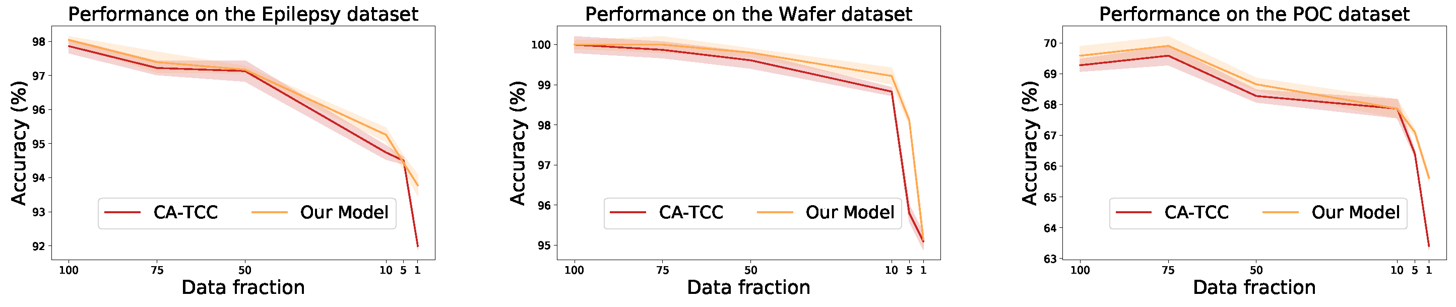
As illustrated in Figure 2, we conduct classification generalization experiments on the Epilepsy, Wafer, and POC datasets, using various labeled data fractions (1%, 5%, 50%, 75%, and 100%). CA-TCC is used as the baseline comparison method, as it employs a similar architecture for contrastive learning and builds a temporal auto-regressive module for classification. The proposed approach consistently outperforms CA-TCC, achieving higher accuracy across all data fractions. The curve representing our method consistently lies above that of the baseline, demonstrating its superior performance. Taking the POC dataset as an example, the standard deviations of the model in different data proportions are [0.1, 0.06, 0.07, 0.09, 0.08, 0.1], while the standard deviations of the proposed model are [0.06, 0.04, 0.03, 0.03, 0.1, 0.1], which demonstrates the robustness of the proposed model.

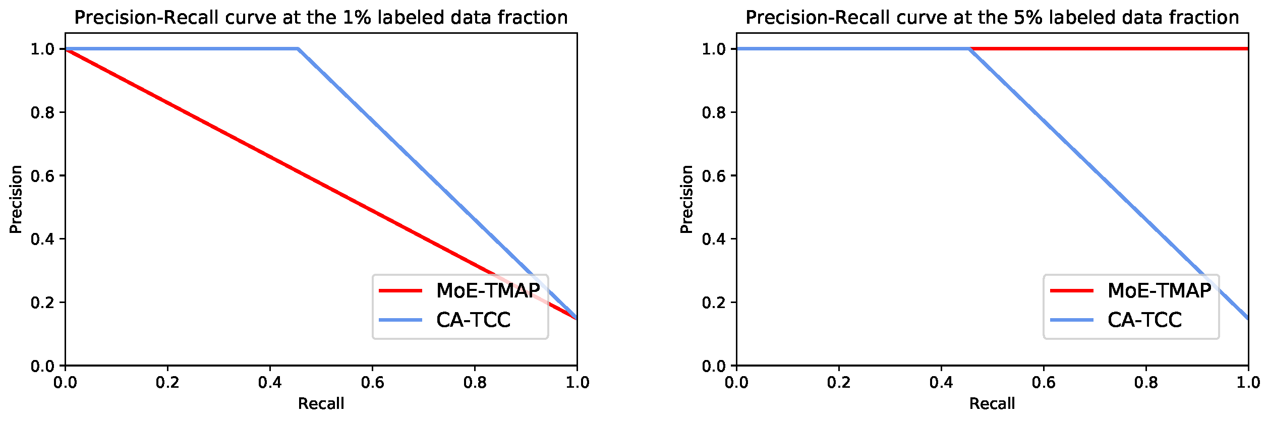
Figure 3 presents the precision–recall curves of the proposed method compared to CA-TCC on the power grid dataset. The curve for EXT-PACL declines gradually with minimal fluctuations, indicating stable performance. Overall, these results demonstrate the strong generalization ability of the proposed approach in semi-supervised time-series classification tasks.

4.6. Ablation Study

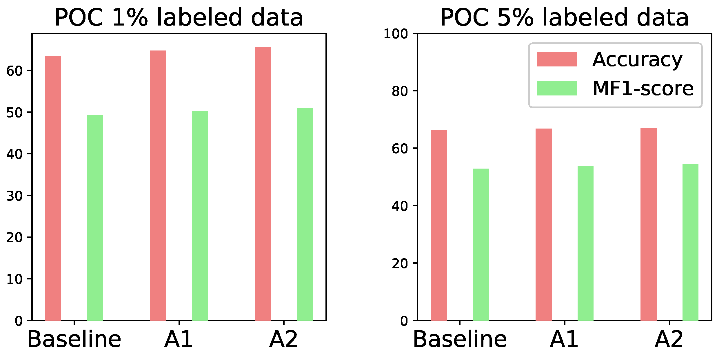
An ablation study was conducted to evaluate the contributions of the proposed design, as illustrated in Figure 4. The baseline model implements contrastive learning following the CA-TCC framework. Next, the MoE-Enhanced Transformer Encoder module was incorporated to enable richer feature interactions, resulting in variant A1. Finally, the prototype-aware contrastive learning strategy was applied, forming variant A2. As shown in Figure 4, compared to the baseline, variant A1 achieves Top-1 accuracies of 64.78% and 66.8% and MF1-scores of 50.19% and 53.9% under 1% and 5% labeled data settings, respectively. Building upon the MoE-Enhanced Transformer Encoder, the full proposed method further improves Top-1 accuracy by 2.22% and 0.7%, and MF1-score by 1.65% and 1.72%, demonstrating the effectiveness of both the MoE integration and the prototype-aware contrastive learning strategy.

Then, we empirically evaluate the effect of varying the number of experts. The model based on softmax routing is defined as E-PACL and is used for comparison. As shown in

Table 2. Effectiveness Evaluation of Various MoE Routing.

Datasets	Epilepsy		Power
Methods	Accuracy	MF1-Score	Accuracy	MF1-Score
1% of labeled data
CA-TCC	63.4 ± 0.4	49.3 ± 0.7	69.9 ± 0.4	67.9 ± 0.6
E-PACL(2)	63.2 ± 0.3	48.8 ± 0.5	70.4 ± 0.5	68.2 ± 0.4
ExT-PACL(2)	64.1 ± 0.2	50.1 ± 0.8	70.4 ± 0.6	68.8 ± 0.4
E-PACL(4)	64.1 ± 0.2	49.7 ± 0.5	70.2 ± 0.6	70.2 ± 0.2
ExT-PACL(4)	65.6 ± 0.3	50.4 ± 0.5	71.7 ± 0.2	69.4 ± 0.7
E-PACL(8)	63.2 ± 0.3	48.2 ± 0.8	70.1 ± 0.2	67.9 ± 0.2
ExT-PACL(8)	64.2 ± 0.3	49.8 ± 0.5	71.2 ± 0.3	68.6 ± 0.3
5% of labeled data
CA-TCC	66.4 ± 0.3	52.8 ± 0.3	76.8 ± 0.6	74.1 ± 0.7
E-PACL(2)	66.5 ± 0.2	53.0 ± 0.2	77.5 ± 0.4	75.5 ± 0.2
ExT-PACL(2)	66.9 ± 0.6	52.9 ± 0.5	77.2 ± 0.6	76.4 ± 0.5
E-PACL(4)	66.3 ± 0.2	52.3 ± 0.6	77.8 ± 0.6	76.9 ± 0.4
ExT-PACL(4)	67.1± 0.2	53.5 ± 0.3	78.7 ± 0.3	78.2 ± 0.5
E-PACL(8)	65.7 ± 0.2	52.9 ± 0.4	75.8 ± 0.6	76.2 ± 0.3
ExT-PACL(8)	66.2 ± 0.4	53.4 ± 0.5	76.9 ± 0.2	77.8 ± 0.7

, increasing the number of experts improves accuracy and MF1-score up to $E=4$, beyond which performance gains saturate. Training time and model parameters increase linearly. Therefore, $E=4$ strikes a balance between model expressivity and computational efficiency.

As shown in

Table 3. Training and Inference Time Complexity Analysis.

Datasets	Methods	Params	Params (One Forward)	Train (ms/it)	Infer (ms/it)
POC	CA-TCC	453.58 K	703.86 M	86.91	9.97
	ExT-PACL	520.14 K	704.53 M	92.21	10.38
power	CA-TCC	340.81 K	356.72 M	61.30	7.63
	ExT-PACL	407.37 K	359.46 M	77.03	8.52

, ExT-PACL contains slightly more parameters than CA-TCC; the increase in single forward-pass time and inference latency is small. The prototype update mechanism is only used during training and does not introduce extra overhead during inference. Consequently, the inference complexity of ExT-PACL is close to that of CA-TCC, while achieving consistently better classification performance and stronger generalization ability.

4.7. Sensitivity Analysis

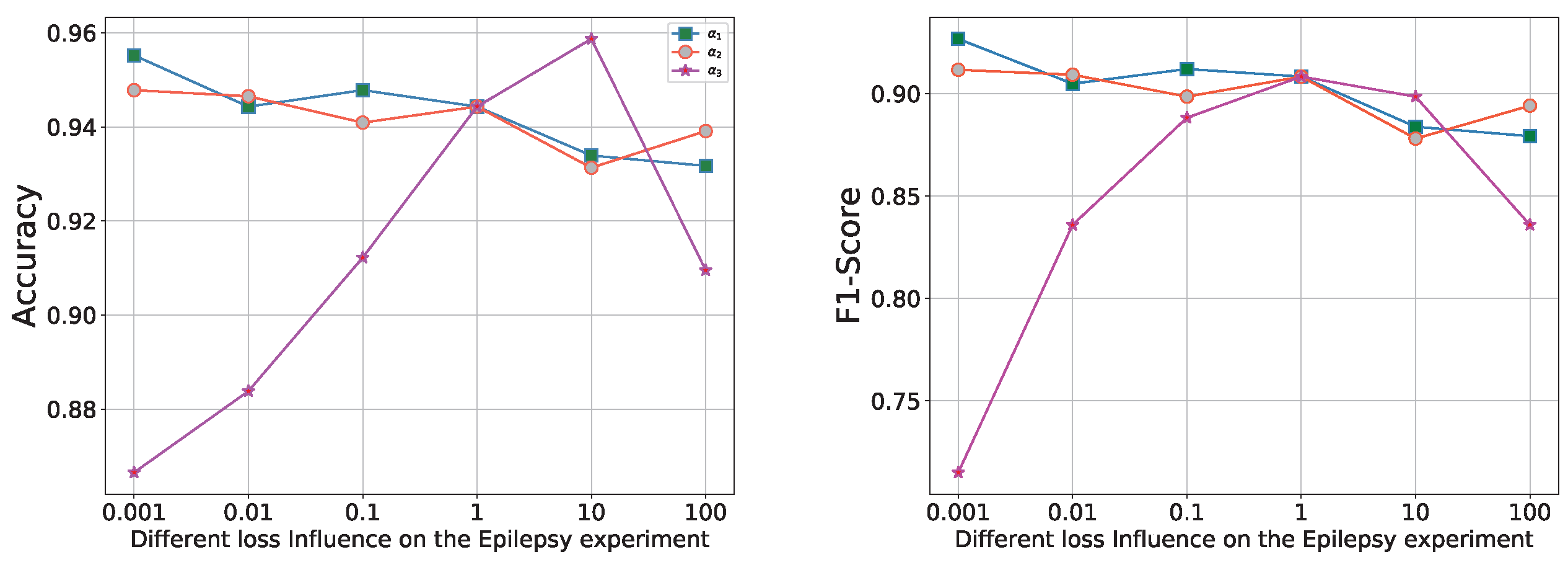
Three hyperparameters (${\alpha }_1$, ${\alpha }_2$, and ${\alpha }_3$) are respectively analyzed, including cross-entropy loss weight, sample-wise contrastive loss weight, and prototype-aware contrastive loss weight. The values of all weights are selected from [0.001, 0.01, 0.1, 1, 10, 100]. As shown in Figure 5, the hyperparameter ${\alpha }_1$ has the most important impact for the classification performance.

5. Conclusions

Semi-supervised contrastive learning for time-series classification (TSC) often suffers from limited generalization across diverse temporal patterns and insufficient guidance from latent category information, leading to sub-optimal feature representations. To overcome these challenges, we propose the Expert-Transformer with Prototype-Aware Contrastive Learning (ExT-PACL), a novel framework that integrates an uncertainty-guided Mixture-of-Experts (MoE) module within a Transformer encoder to adaptively capture complex temporal dynamics. An expert balancing mechanism ensures equitable utilization of all experts, preventing collapse and enhancing robustness. Furthermore, a prototype-aware contrastive loss iteratively computes class prototypes to guide both labeled and high-confidence unlabeled samples, embedding categorical semantics and improving discriminative power. Extensive experiments on multiple benchmark datasets demonstrate that ExT-PACL achieves state-of-the-art performance, particularly in low-label settings, highlighting its effectiveness in addressing intra-class variability and distribution shifts in semi-supervised TSC.

References

1. Yehuda, Y.; Freedman, D.; Radinsky, K. Self-supervised Classification of Clinical Multivariate Time Series using Time Series Dynamics. In Proceedings of the 29th ACM SIGKDD Conference on Knowledge Discovery and Data Mining, Long Beach, CA, USA, 2023; KDD’23; ACM: New York, NY, USA, 2023; pp. 5416–5427. [Google Scholar] [CrossRef]
2. Dzaferagic, M.; Marchetti, N.; Macaluso, I. Fault Detection and Classification in Industrial IoT in Case of Missing Sensor Data. IEEE Internet Things J. 2021, 9, 8892–8900. [Google Scholar] [CrossRef]
3. Oliveira, M.; Costa, G. Quantitative portfolio optimization framework with market regimes classification, probabilistic time series forecasting, and hidden Markov models. Digit. Financ. 2025, 7, 553–603. [Google Scholar] [CrossRef]
4. Müller, P.N.; Müller, A.J.; Achenbach, P.; Göbel, S. IMU-Based Fitness Activity Recognition Using CNNs for Time Series Classification. Sensors 2024, 24, 742. [Google Scholar] [CrossRef] [PubMed]
5. Chen, W.; Shi, K. Multi-scale Attention Convolutional Neural Network for time series classification. Neural Netw. 2021, 136, 126–140. [Google Scholar] [CrossRef] [PubMed]
6. Liu, H.; Yang, D.; Liu, X.; Chen, X.; Liang, Z.; Wang, H.; Cui, Y.; Gu, J. TodyNet: Temporal dynamic graph neural network for multivariate time series classification. Inf. Sci. 2024, 677, 120914. [Google Scholar] [CrossRef]
7. Foumani, N.M.; Tan, C.W.; Webb, G.I.; Salehi, M. Improving position encoding of transformers for multivariate time series classification. Data Min. Knowl. Discov. 2024, 38, 22–48. [Google Scholar] [CrossRef]
8. Oord, A.; Li, Y.; Vinyals, O. Representation Learning with Contrastive Predictive Coding. arXiv 2018, arXiv:1807.03748. [Google Scholar]
9. Chen, T.; Kornblith, S.; Norouzi, M.; Hinton, G. A Simple Framework for Contrastive Learning of Visual Representations. In Proceedings of the 37th International Conference on Machine Learning, Online, 13–18 July 2020; Daumé, H., III, Singh, A., Eds.; PMLR (Proceedings of Machine Learning Research): Vienna, Austria, 2020; Volume 119, pp. 1597–1607. [Google Scholar]
10. Eldele, E.; Ragab, M.; Chen, Z.; Wu, M.; Kwoh, C.K.; Li, X.; Guan, C. Self-Supervised Contrastive Representation Learning for Semi-Supervised Time-Series Classification. IEEE Trans. Pattern Anal. Mach. Intell. 2023, 45, 15604–15618. [Google Scholar] [CrossRef] [PubMed]
11. Xing, H.; Xiao, Z.; Dawei, Z.; Luo, S.; Dai, P.; Li, K. SelfMatch: Robust semisupervised time-series classification with self-distillation. Int. J. Intell. Syst. 2022, 37, 8583–8610. [Google Scholar] [CrossRef]
12. Liu, C.; Guan, D.; Yuan, W.; Koc, C.K. ITS2Graph: Graph-based generative adversarial learning for imbalanced time series classification. Neural Netw. 2025, 191, 107770. [Google Scholar] [CrossRef] [PubMed]
13. Pei, E.; Zhao, W.; Hu, Z.; He, L.; Ning, H.; Chen, H. Classifier ensemble based source-free domain adaptation for time series classification. Knowl. Based Syst. 2025, 330, 114584. [Google Scholar] [CrossRef]
14. Liu, H.; Zhang, F.; Huang, X.; Wang, R.; Xi, L. Bidirectional consistency with temporal-aware for semi-supervised time series classification. Neural Netw. 2024, 180, 106709. [Google Scholar] [CrossRef] [PubMed]
15. Eldele, E.; Ragab, M.; Chen, Z.; Wu, M.; Kwoh, C.K.; Li, X.; Guan, C. Time-Series Representation Learning via Temporal and Contextual Contrasting. In Proceedings of the Thirtieth International Joint Conference on Artificial Intelligence (IJCAI-21), Virtual, 19–27 August 2021. [Google Scholar]
16. Zhang, J.; Dai, Q.; Ye, R. iBACon: imBalance-Aware Contrastive Learning for Time Series Forecasting. IEEE Trans. Knowl. Data Eng. 2025, 37, 5967–5982. [Google Scholar] [CrossRef]
17. Liu, M.; Sheng, H.; Zhang, N.; Zhao, P.; Yi, Y.; Jiang, Y.; Dai, J. DSDCLNet: Dual-stream encoder and dual-level contrastive learning network for supervised multivariate time series classification Multivariate Time Series Classification Gated Recurrent Unit Multiscale Convolutional Neural Network Dual-Stream Encoder Contrastive Learning. Knowl. Based Syst. 2024, 292, 111638. [Google Scholar] [CrossRef]
18. Cao, Y.; Fan, L.; Wang, W.; He, Y. Machine learning-driven acceleration of Mg-MOF-74 synthesis optimization for enhanced CO2 adsorption. Sep. Purif. Technol. 2026, 398, 138172. [Google Scholar] [CrossRef]
19. Yan, H.; Ye, L.; Zhou, T.; Li, Z.H.; Ye, T.; Zhang, F.; Liu, C.L. Physics-informed neural network for predicting multi-row film cooling superposition using Fourier transform and attention mechanism. Phys. Fluids 2025, 37, 065174. [Google Scholar] [CrossRef]
20. Andrzejak, R.; Lehnertz, K.; Mormann, F.; Rieke, C.; David, P.; Elger, C. Indications of nonlinear deterministic and finite-dimensional structures in time series of brain electrical activity: Dependence on recording region and brain state. Phys. Rev. E Stat. Nonlinear Soft Matter Phys. 2002, 64, 061907. [Google Scholar] [CrossRef] [PubMed]
21. Sarkar, P.; Etemad, A. Self-Supervised ECG Representation Learning for Emotion Recognition. IEEE Trans. Affect. Comput. 2020, 13, 1541–1554. [Google Scholar] [CrossRef]
22. Tarvainen, A.; Valpola, H. Mean teachers are better role models: Weight-averaged consistency targets improve semi-supervised deep learning results. In Proceedings of the Advances in Neural Information Processing Systems; Guyon, I., Luxburg, U.V., Bengio, S., Wallach, H., Fergus, R., Vishwanathan, S., Garnett, R., Eds.; Curran Associates, Inc.: Nice, France, 2017; Volume 30. [Google Scholar]
23. Li, J.; Socher, R.; Hoi, S.C.H. DivideMix: Learning with Noisy Labels as Semi-supervised Learning. arXiv 2020, arXiv:2002.07394. [Google Scholar]
24. Fan, H.; Zhang, F.; Wang, R.; Huang, X.; Li, Z. Semi-Supervised Time Series Classification by Temporal Relation Prediction. In Proceedings of the ICASSP 2021–2021 IEEE International Conference on Acoustics, Speech and Signal Processing (ICASSP); IEEE: Piscataway, NJ, USA, 2021; pp. 3545–3549. [Google Scholar] [CrossRef]
25. Sohn, K.; Berthelot, D.; Carlini, N.; Zhang, Z.; Zhang, H.; Raffel, C.A.; Cubuk, E.D.; Kurakin, A.; Li, C.L. FixMatch: Simplifying Semi-Supervised Learning with Consistency and Confidence. In Proceedings of the Advances in Neural Information Processing Systems; Larochelle, H., Ranzato, M., Hadsell, R., Balcan, M.F., Lin, H., Eds.; Curran Associates, Inc.: Nice, France, 2020; Volume 33, pp. 596–608. [Google Scholar]
Figure 1. The overall framework of the proposed approach.
Electronics 15 02303 g001
Figure 2. The generalization experiment conducted on the three datasets at different data fractions. Shaded areas in the figure represent the standard deviation trends.
Electronics 15 02303 g002
Figure 3. The precision–recall curves of our proposed approach compared with CA-TCC on the power grid dataset.
Electronics 15 02303 g003
Figure 4. The ablation study for the proposed design.
Electronics 15 02303 g004
Figure 5. The analysis of default hyperparameters.
Electronics 15 02303 g005