1. Introduction
Since the 21st century, advancements in high-performance semiconductor power devices and permanent magnet materials have laid a solid foundation for the application of permanent magnet synchronous motors (PMSMs) in industry. Compared with induction motors, PMSMs offer significant advantages in power density and mechanical efficiency [
1,
2]. In multiphase motors, particularly dual three-phase PMSMs, their torque ripple, system stability, power density, and fault tolerance are further enhanced compared with three-phase motors [
3,
4,
5]; consequently, they have been widely adopted in electric vehicles, aerospace, wind power generation, and other fields [
6,
7,
8].
Model predictive control (MPC) has developed rapidly over the past decade due to its conceptual simplicity, fast dynamic response, and ease of multi-objective optimization. Depending on the control objective, MPC can be divided into model predictive torque control (MPTC) and model predictive current control (MPCC). Based on the voltage vector set, it can be further classified into continuous-set MPC and finite-set MPC. Among these, MPCC has been successfully applied to address common-mode voltage issues in multiphase drive systems. However, conventional MPCC suffers from inherent drawbacks when applied to multiphase PMSM drive systems, including severe harmonic currents, difficult-to-determine weighting factors, high computational burden, and variable switching frequency [
9,
10,
11,
12,
13]. To suppress harmonic currents, Ref. [
11] proposed an MPCC method based on virtual voltage vectors. Ref. [
12] achieved constant-switching-frequency predictive torque control through duty-cycle optimization, while Ref. [
13] fixed the switching frequency and reduced the computational burden to a certain extent. Although these improvements have achieved certain effects, they remain highly dependent on motor parameters—parameters that vary with operating conditions such as temperature and mechanical vibration, while inverter dead-time and DC-link voltage fluctuations also impair accurate modeling [
14,
15,
16]. Therefore, reducing MPC’s parameter sensitivity has become a key challenge in this field.
To address the parameter sensitivity issue, researchers have explored anti-interference MPC methods. Among them, model-free predictive current control (MFPCC) has developed particularly rapidly in the past five years because it is independent of system models, completely parameter-free, and robust. French scholars first proposed an MFPCC method based on an ultra-local model. They used differential algebra to estimate the nonlinear part of the model [
17], providing a new idea to overcome parameter dependence. However, the differential algebra approach involves numerous parameters and complicated tuning. Li and colleagues implemented a conventional differential-algebra-based MFPCC for PMSMs, which enables the feedback current to track the reference value even under parameter mismatch [
18].
Nevertheless, such methods have obvious limitations: poor steady-state performance, high demands on sensor accuracy, and large estimation errors associated with the algebraic method. To address this issue, various observers have been introduced to estimate the nonlinear part of the ultra-local model. For example, the extended-observer-based MFPCC reduces the number of tunable parameters and improves steady-state performance [
19]; the sliding-mode-observer-based (SMO) design can accurately estimate the current change rate and combine an effective voltage vector with a zero vector within one sampling period [
20]. However, the gains of these observers are typically fixed. They cannot adapt to varying operating conditions, while the chattering problem inherent to sliding-mode observers is difficult to eliminate. In addition, the continuous-set-modulation-based MFPCC [
21] improves steady-state performance but reduces dynamic response due to the modulator. Ref. [
22] implemented an extended-observer-based MFPCC for dual three-phase PMSMs on a low-cost processor, which can adjust the amplitude of the optimal voltage vector but cannot change its arbitrary angle, thereby limiting current tracking capability.
In summary, existing MFPCC methods still have notable deficiencies in tracking capability, steady-state performance, and flexibility in voltage vector regulation. No existing method effectively expands the voltage modulation region to reduce current and torque ripple while maintaining the advantages of model-free control. To fill this gap, this paper proposes a model-free predictive current control strategy based on an EKO and modulated virtual voltage vectors. Unlike existing fixed-gain observers, the EKO provides an adaptive gain coefficient matrix based on the minimum-variance criterion, enabling optimal estimation of the nonlinear part of the ultra-local model and thereby achieving better control performance under parameter mismatch. Meanwhile, the introduction of MVVs expands the modulation region and effectively suppresses current and torque ripple. Furthermore, the switching sequence is implemented using triangular wave carriers, facilitating deployment on low-cost microprocessors. Experimental results show that the proposed method exhibits superior robustness and steady-state performance under operating conditions, including parameter mismatches and dynamic load variations.
The remainder of this paper is organized as follows:
Section 2 introduces the mathematical model of the DT-PMSM and the conventional MPCC method based on virtual voltage vectors;
Section 3 elaborates on the proposed MFPCC method;
Section 4 experimentally verifies the steady-state and dynamic performance as well as the computational burden of the proposed method under both parameter-matched and -mismatched conditions;
Section 5 summarizes the full paper.
3. The Proposed Method
As shown in Equations (6) and (8)–(10), both the predictive model calculations and the duty-cycle computations depend critically on motor parameters. Any mismatch in these parameters will directly degrade the model predictive controller’s control performance. To enable accurate analysis, this section establishes a mathematical model of motor parameter mismatch.
3.1. The Mathematical Model of Motor Parameter Mismatch
The MPCC method suffers from performance degradation when motor parameters are mismatched [
14]. This section presents a model-free predictive control approach based on an EKO that enables current prediction and duty-cycle calculation without relying on motor parameters. Factors such as inductance saturation, mechanical vibration, and temperature rise may cause variations in motor parameters, including inductance, resistance, and flux linkage. To account for these effects, a mathematical model of the motor under parameter mismatch is established. Here, let Δ
ψf, Δ
Ld, Δ
Lq, and Δ
Rs represent the mismatch degrees of the permanent magnet flux linkage,
d-axis inductance,
q-axis inductance, and stator resistance, respectively. Here, only the mathematical model on the
d-q axis needs to be considered, as the synthesis of the MVV is introduced in the next section, and the average value of the MVV on the
x-y plane is zero. Therefore, the mathematical model of the motor in the
x-y plane does not need to be considered. The voltage equation of the dual-three-phase PMSM mathematical model, considering unknown interference terms and motor parameter mismatch, is specifically expressed as follows:
where Δ
Rs, Δ
Ls, and Δ
ψf are the changes in resistance, inductance, and flux linkage, respectively. Moreover,
λd and
λq are the unknown interference terms. By modifying Equation (12), the dynamic equation for the current can be obtained as follows:
Next, the influence of motor parameter mismatch on the MPCC method was investigated. Several sets of simulation studies were conducted under the working conditions of a speed of 1500 r/min and a load of 6 Nm.
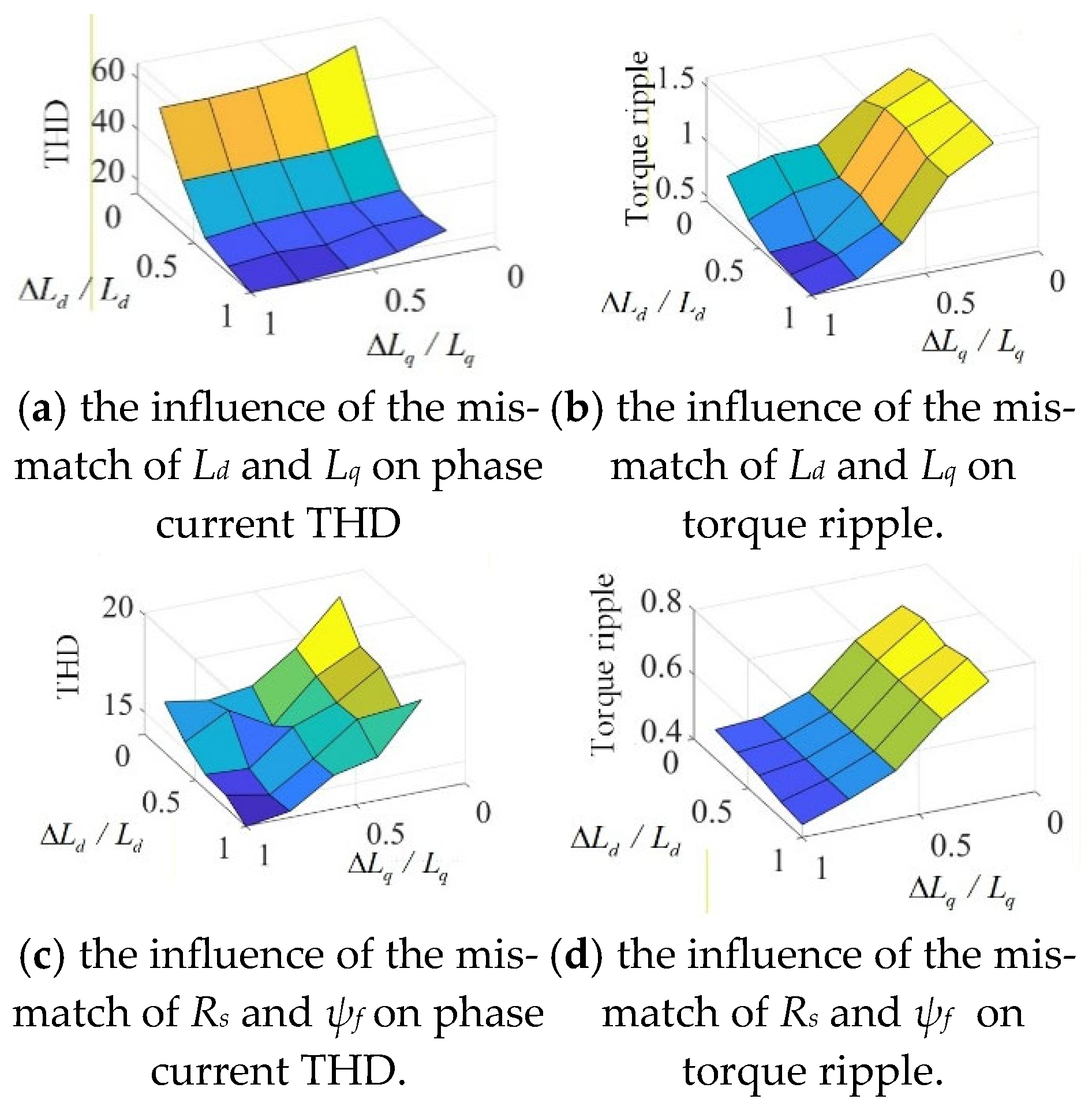
Figure 4 presents the analysis diagram of the influence of motor parameter mismatch on the phase current total harmonic distortion (THD) and torque ripple. Specifically,
Situation 1:
Figure 4a shows the influence of the mismatch of
Ld and
Lq on phase current THD.
Situation 2:
Figure 4b shows the influence of the mismatch of
Ld and
Lq on torque ripple.
Situation 3:
Figure 4c shows the influence of the mismatch of
Rs and
ψf on phase current THD.
Situation 4:
Figure 4d shows the influence of the mismatch of
Rs and
ψf on torque ripple.
As shown in
Figure 4, compared with the
Ld direction, the variation slope of the THD in the
Lq direction is steeper, and the phase current THD varies from 14.05% to 56%. This indicates that the
Lq parameter mismatch has a significant impact on the THD. Similarly, the variation range of torque ripples in the
Lq direction is from 0.45 Nm to 1.52 Nm, which proves that the influence of
Lq parameter mismatch on torque ripple is also greater than that of
Ld. The parameter mismatch of
Rs has no obvious effect on torque ripple, and its influence on THD is limited to a 3% range. The parameter mismatch of
ψf has an effect on the THD of phase current, which is limited to a variation range of 6%, and its influence on torque ripple is within the range of 0.4 Nm. In conclusion, compared with mismatches in resistance and flux linkage parameters, mismatches in inductance parameters have the greatest impact on THD and torque ripple.
3.2. The Modulated Virtual Voltage Vector
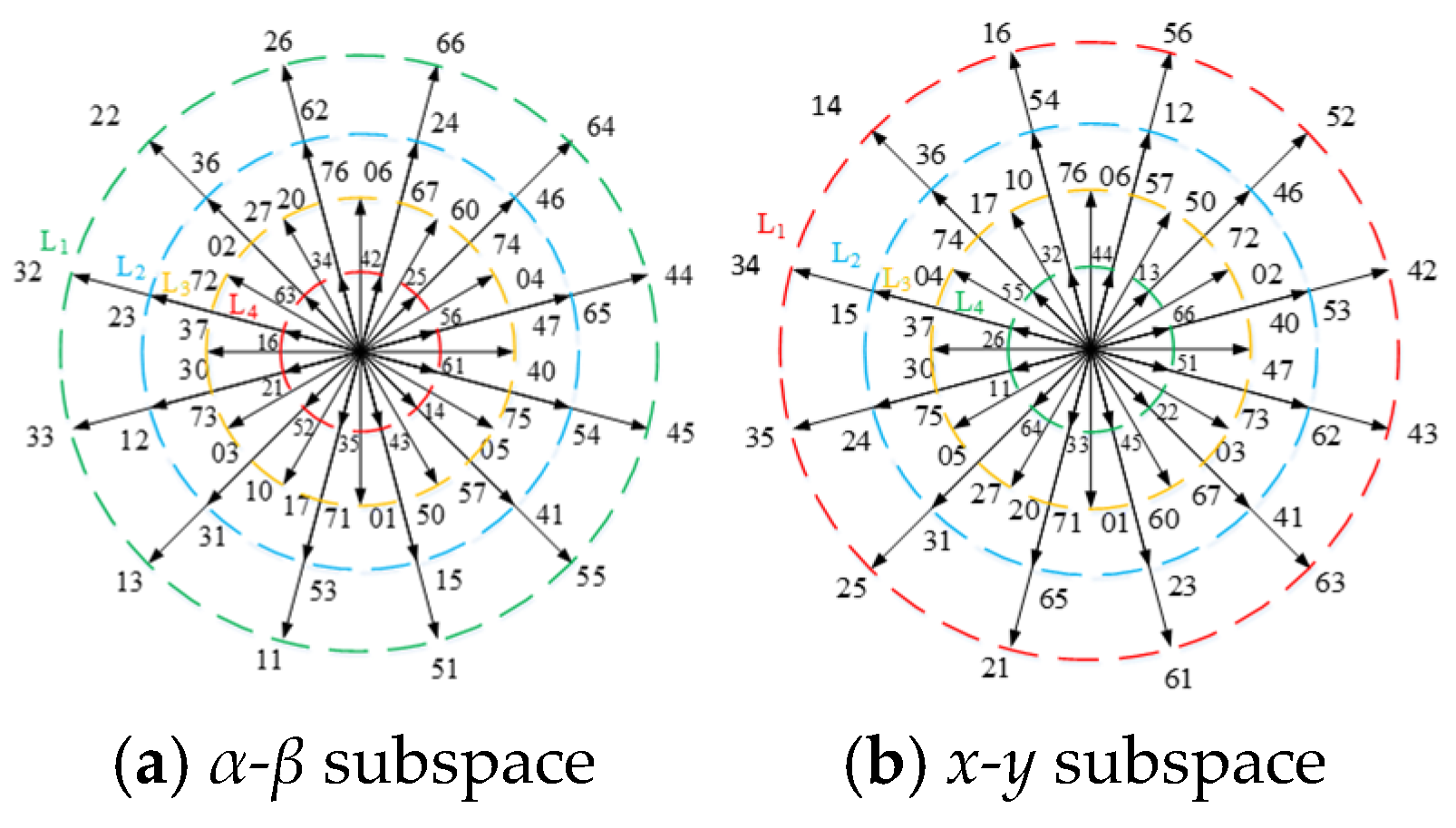
Although the virtual voltage vector described in
Section 2.2 can effectively suppress harmonic current, the discrete voltage vector in a finite control set limits the modulation range, thereby affecting the improvement in control performance [
23]. In this section, the MVV is proposed to improve the modulation range.
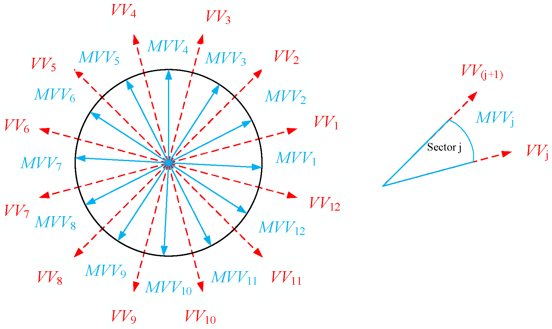
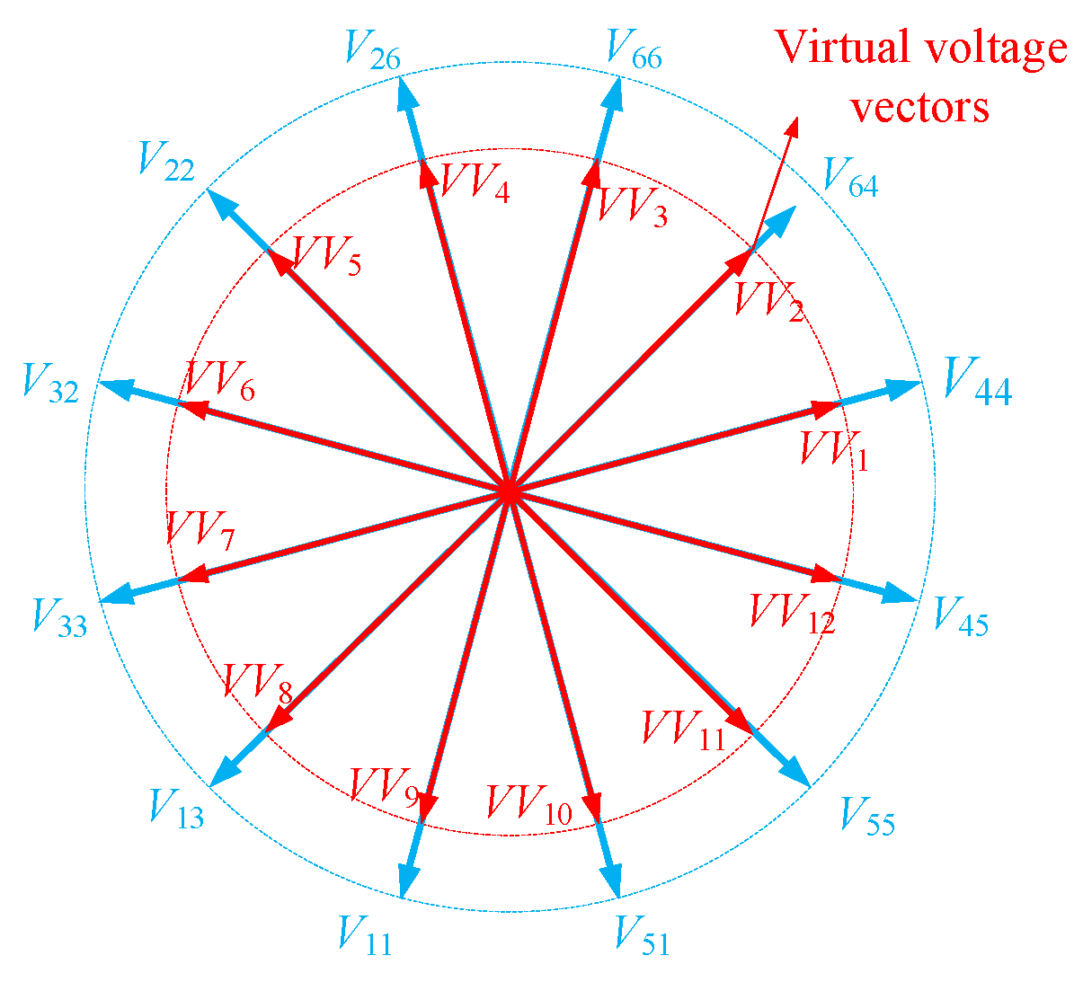
An MVV based on online synthesis is proposed, which covers the entire regular dodecagon modulation region. Each MVV is composed of zero vectors and two adjacent virtual voltage vectors. The distribution of the MVVs is shown in
Figure 5, and they are named MVV
1-MVV
12. The synthesis of the MVVs can be expressed as follows:
dj, dj+1, and d0 represent the duty cycle of two adjacent virtual voltage vectors and the zero vector, respectively. Here, VVj, VV(j+1), and V0 are the first, second, and zero virtual voltage vectors, respectively.
3.3. The Ultra-Local Model Design
To mitigate the reliance of MPC methods on the accuracy of motor parameters, an ultra-local model of the motor can be derived based on the dynamic equations of the
d-axis and
q-axis currents under mismatched motor parameters and unknown disturbances, as formulated in
Section 3.1, and combined with the ultra-local model theory proposed in Ref. [
22]. This ultra-local model is specifically expressed as follows:
where
ξd = 1/
Ld, and
ξq= 1/
Lq. The nonlinear disturbance terms
and
are specifically expressed as Equation (17).
The nonlinear disturbance terms cannot be calculated directly using formulas but must be estimated using an observer, as detailed in
Section 3.5. By discretizing Equation (16) with the forward Euler method and applying a one-step delay compensation, the ultra-local model for predicting the current can be derived as Equation (18)
where
Ts represents the sampling period. Specifically,
Compared to Equation (5), Equation (18) eliminates the need for motor parameters in the predictive model. Here, ξd and ξq represent the reciprocals of Ld and Lq values, respectively. However, due to potential discrepancies between the actual and nominal motor parameters, ξd and ξq require correction via a trial-and-error approach.
The optimal voltage vector among 12 MVVs is selected by Equation (7). As can be seen from Equations (18) and (19), compared with the current prediction part of the MPC method,
id(
k + 1) and
iq(
k + 1) are only related to voltage,
Fd,
Fq, and scale factors; they do not require motor parameters.
Fd and
Fq are obtained from EKO observations described in
Section 3.5. The EKO continuously corrects the predicted current via feedback, reduces instability caused by parameter perturbations, and improves control accuracy. Therefore, control performance can be guaranteed when motor parameters are mismatched.
3.4. Calculate the Duty Cycle Without Motor Parameters
The duty-cycle calculation proposed in
Section 2.2 relies on accurate motor parameters. Parameter mismatches may adversely affect current tracking performance and prediction accuracy. Based on the ultra-local model introduced in
Section 3.2, a duty-cycle calculation method without parameters is designed in this section, which updates the current variation rate for each candidate voltage vector at every control cycle without requiring specific motor parameters. The predicted current values obtained from Equation (18) are then substituted into the cost function Equation (7) to select the optimal voltage vector. This approach also mitigates the impact of motor parameter mismatch on the selection of the optimal voltage vector.
To make the
d- and
q-axis current track to the given value without error, the deadbeat current control principle calculates the action time of each virtual voltage vector:
where
Ts is the sampling period;
and
represent the current slopes on the
d- and
q-axis of the first virtual voltage vector;
and
represent the current slopes on the
d- and
q-axis of the second virtual voltage vector; and
and
represent the current slopes on the
d- and
q-axis when the zero vector is applied. The current slopes of three vectors are obtained using Equation (16) of the discrete system ultra-local model:
where
z represents the
d- and
q-axes.
The simultaneous equation can be solved to calculate the action time of the virtual voltage vector:
where
When the sum of
tj and
tj+1 is greater than
Ts, it is necessary to ensure the effectiveness of the applied voltage and correct
tj and
tj+1:
3.5. Observation of Nonlinear Disturbance Terms
The traditional MFPCC method uses differential algebra to estimate
Fd and
Fq. To improve the accuracy of the ultra-local model, the proposed method designs an EKO to estimate
Fd and
Fq. The EKO can accurately estimate the system state from the measured data.
Fd and
Fq in the ultra-local model are defined as extended state variables. The EKO is designed based on the ultra-local model, as follows:
where
Using the first-order Euler formula to discretize Equation (27), the following discretization equation can be obtained:
The correlation Jacobian matrix is calculated as follows:
The EKO can be roughly divided into the prediction and update stages. The prediction stage consists of two parts, including the predicted value of the state variable and the calculation of the error covariance matrix:
First, the following definitions are given: Ts is the sampling period, “~” is the predicted value, and “” is the estimated value.
- (1)
To predict the state variable, use the output and the state estimate of the previous moment to predict the state variable of the next moment:
- (2)
Calculate the error covariance matrix:
where
Q represents the process performance noise covariance matrix.
The update stage has three steps, including the calculation of the gain matrix, the calculation of the best estimate, and the update of the error covariance matrix:
- (1)
Calculate the gain matrix K(k):
- (2)
Calculate the best estimate:
- (3)
Update the error covariance matrix to calculate the next error covariance matrix:
The selection of the three initial matrices, P, Q, and R, is critical, as the control performance of the driving system depends on their parameter design. To achieve an appropriate bandwidth gain, a trade-off must be made between sampling error and the control objective’s characteristics. Here is the specific parameter tuning process:
The initial value of
P has minimal impact on steady-state performance and rise time, but affects the system’s overshoot magnitude. A common choice is
R characterizes the measurement noise. If measured values from sensors such as current sensors exhibit significant deviations,
R generally needs to be set to a larger value. Collect 2000 samples of the current sensor output at a standstill. Compute the variance. The noise equivalent current variance is approximately
. Thus,
Q represents the noise intensity process and reflects the degree of model mismatch. The system’s dynamic response accelerates with increasing gain matrix magnitude, though higher values also introduce greater noise. Let
, where
corresponds to the current states and
to the disturbance states. The tuning heuristic is: Start with small values. Perform a load step change. If the current response is sluggish, increase
until the settling time meets the requirement. If high-frequency ripples appear in the current, reduce
because it is too large;
is usually one order of magnitude smaller than
because the ultra-local model already describes the current dynamics well, whereas the disturbances may vary. For our system, the following values give the best trade-off:
The scaling factors are defined as and . Although nominal values can be obtained from the motor datasheet, the actual inductances vary with load. The following steps are performed: set and using the nameplate inductances. Set the EKO disturbance estimates to zero initially. Adjust to make the steady-state -axis current zero. Adjust so that the -axis current matches its small reference. Apply rated load. Repeat the adjustment. Verify the current THD and tracking error at 50% and 100% loads. If the variation is large, take the average of the values obtained under different loads. The empirical values used in this paper are and .
3.6. Convergence Analysis of the EKO
Lemma 1. For the above linear time-invariant system, if (F,H) is observable, , and , then the estimation error covariance matrix of the standard Kalman filter converges exponentially to a unique positive-definite steady-state solution . Moreover, the estimation error is mean-square bounded and asymptotically stable.
Proof. The observability matrix has full rank; hence, the system is observable. According to Kalman filtering theory, the discrete algebraic Riccati equation,
has a unique positive-definite symmetric solution. The error covariance
converges geometrically to
from any initial
. The estimation error dynamics are
where
collects noise and linearization errors. Because
is bounded and the spectral radius of
is less than one, the error system is input-to-state stable.
For the actual nonlinear system, the EKO uses first-order linearization and still guarantees local asymptotic convergence, provided the sampling period is sufficiently small.□
3.7. Stability Analysis of the Current Closed-Loop System
Define the current tracking error as
. Based on the deadbeat principle, the proposed method selects, in each sampling period, an optimal MVV and its duty cycles such that the error at the next instant would be zero under ideal estimation, due to the estimation error
. Moreover, discretization approximations, the actual error dynamics satisfy
where
is the desired voltage,
is the actual voltage applied, and
lumps higher-order terms and quantization errors. Because the MVV covers the entire regular dodecagon modulation region and the duty cycles are computed using the deadbeat principle, ideally
. Thus,
Theorem 1. If the EKO estimation error is uniformly bounded, i.e., there exists a constant such that for all , and , then the current tracking error is uniformly ultimately bounded. The ultimate bound is linear in and .
Proof. Choose the Lyapunov candidate function . Its forward difference is
Using
and
, we obtain
If for some , then for some . Hence eventually enters a neighborhood of zero of radius . Therefore, the tracking error is UUB.
In practice, because the EKO converges, tends to zero in the mean-square sense as increases. The steady-state current error is then dominated by .□
3.8. Sensitivity Analysis of Measurement Noise and Disturbances
The ultra-local model of Equation (16) is written in discrete form with consideration of noise effects:
where
. Measurement noise propagates through the current feedback
and the one-step-ahead prediction
. The EKO state estimation equation is
with
containing noise. From Kalman filter theory, the estimation error covariance
is monotonically positively correlated with the measurement noise covariance
. In the steady state, the Kalman gain
satisfies
When increases, decreases; the observer suppresses noise more heavily but at the cost of slower dynamic response. In this process, the variance of the current prediction error is proportional to . Because the proposed method uses an ultra-local model that does not rely on motor physical parameters, noise is not amplified through differentiation or inversion of inductances, resistances, etc. Moreover, the EKO adaptively adjusts its gain according to the noise covariance, avoiding the excessive high-frequency noise amplification typical of fixed-gain observers.
Thus, a theoretical conclusion can be drawn: the sensitivity . The current tracking error to measurement noise is bounded, and while it depends on the sampling frequency and the design of the matrix, it is not affected by motor parameter mismatches.
The proposed method uniformly models motor parameter mismatches and external disturbances as
. The true nonlinear term in the ultra-local model is
where
denotes the estimate provided by the observer, and
represents the unmodeled component. In the proposed method, the EKO estimates
online. The estimation error dynamics satisfy
where
is the process noise representing the rate of change of
. In steady state, if the system satisfies the uniform observability condition, the mean of the estimation error
is bounded, and its variance is related to
and
.
The torque ripple
can be approximated as a function of current harmonics:
where
is the amplitude of the
-th current harmonic and
is the torque constant. When
increases, the current prediction error grows, leading to larger harmonic currents. However, because the EKO estimates
. In real time, the estimation error does not diverge, and the influence of disturbances on torque ripple is linear and has a finite gain. Specifically, there exists a constant
such that
This theoretical result indicates that the proposed method is inherently robust to parameter mismatches and external disturbances.
3.9. Switching Sequence and Digital Implementation
Ref. [
24] generates a centrally symmetric standard PWM waveform using a triangular carrier; that is, within a control period, the modulator compares the triangular wave carrier with a fixed reference value to form the desired switching sequence. Unfortunately, the output reference voltage vector is inaccurate, which increases the harmonic content to a certain extent.
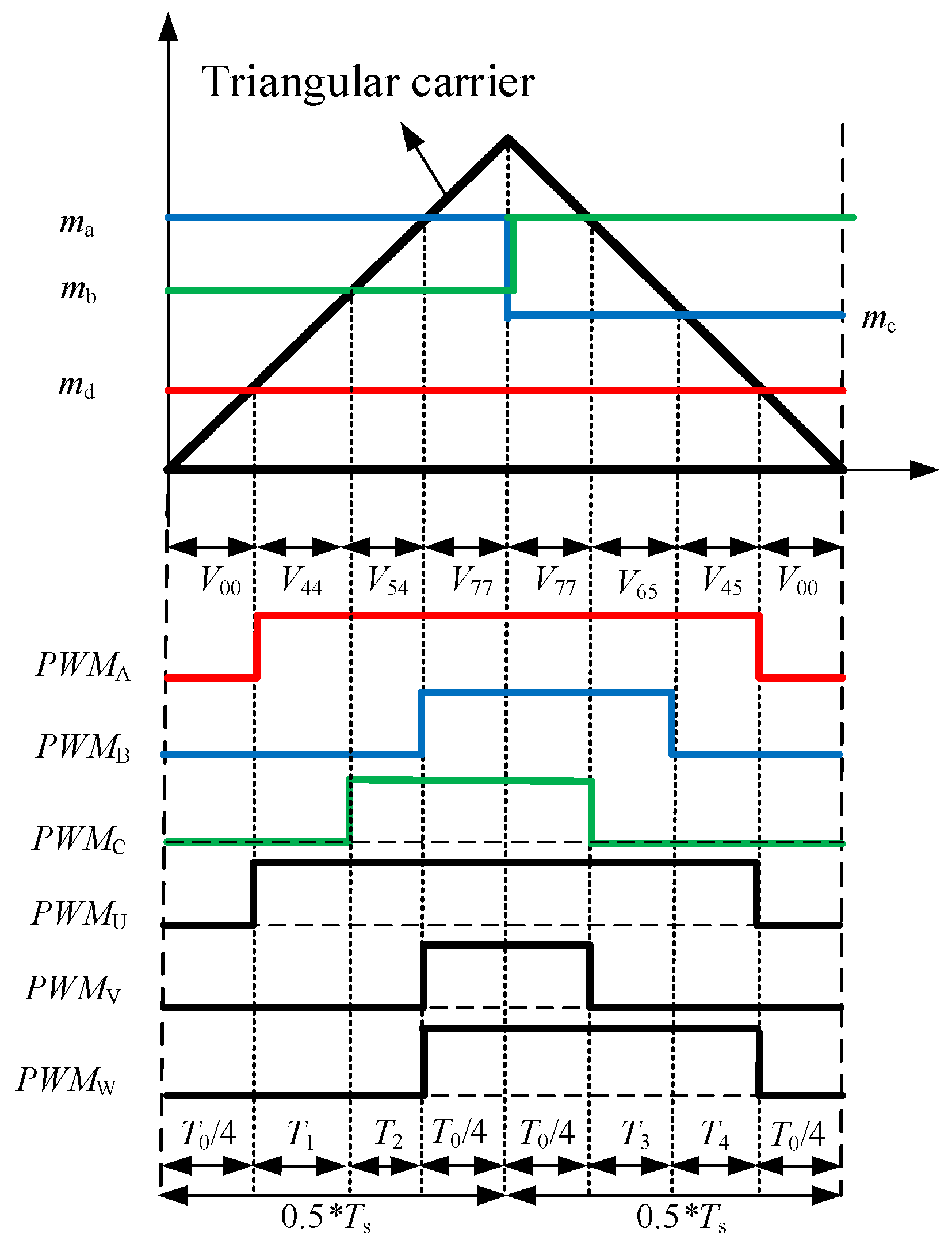
The switching sequence proposed in this paper is asymmetric and can accurately output the reference voltage vector, as shown in
Figure 6.
The asymmetric switching sequence method uses a sawtooth carrier to generate [
24]. The use of triangular carriers to generate asymmetric switching sequences. Specifically, this approach greatly simplifies both comprehension and software implementation within the increment/decrement modes of a DSP. In the CMPA/CMPB registers, the update occurs at
Ts/2, that is, the reference value modulation wave changes to produce an asymmetric PWM signal. The specific way to achieve this is to compare the triangular carrier with four reference values, with each phase corresponding to one or two of them. When the reference value and the triangular carrier value are equal for the first time, the switching signal changes from 0 to 1. When the reference value is equal to the triangular carrier value for the second time, the switching signal changes from 1 to 0, and the asymmetric PWM signal is realized.
As an example,
Figure 6 shows the generation principle of the six-phase switching sequence, and it gives the calculation of reference values
ma,
mb,
mc, and
md:
where
T1,
T2,
T3 and
T4 are the action time of
V44,
V54,
V65 and
V45.
The carrier wave is a triangular wave, and the reference value of the A-phase is consistent before and after two half-periods, which is (
T1 +
T2 +
T3 +
T4)/
Ts. For the B-phase, the reference value is (−
T1 −
T2 −
T3 −
T4)/
Ts in the first half-period and 2 * (
T3 −
T4)/
Ts in the second half-period. For the C-phase, its reference value also changes at
Ts/2; the first half-period is 2 * (
T2 −
T1)/
Ts, and the second half-period is (−
T1 −
T2 −
T3 −
T4)/
Ts. The reference value of the U-phase is consistent with that of A, which is (
T1 +
T2 +
T3 +
T4)/
Ts; the reference wave of the V-phase is also constant in a period, which is (−
T1 −
T2 −
T3 −
T4)/
Ts; the reference value of the W-phase is (−
T1 −
T2 −
T3 −
T4)/
Ts in the first half-period. The second half-period is (
T1 +
T2 +
T3 +
T4)/
Ts.
3.10. Discussion on Modulation Range and Observers
For the sake of convenience in the following elaboration, the proposed method is referred to as the MFPCC-MVVV method.
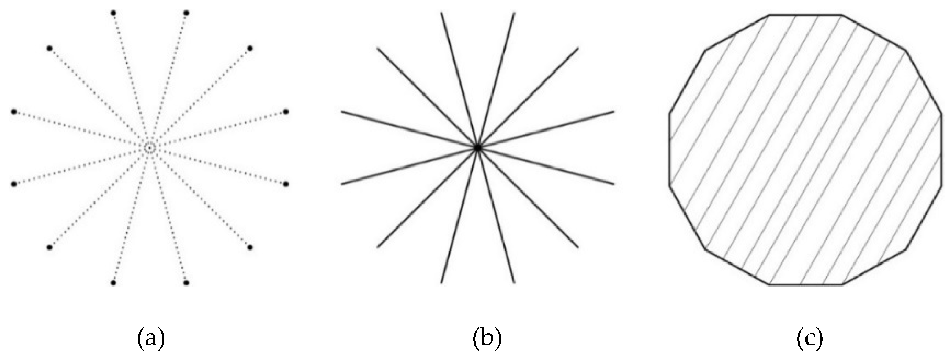
Figure 7 compares the modulation region for the traditional MPCC method (MPCC-TRAD), the traditional MFPCC method with virtual voltage vectors based on duty-cycle modulation (MFPCC-TRAD-VVV), and the MFPCC-MVVV method. In the MPCC-TRAD, since there are only 12 large-voltage vectors and one zero vector in the control set, the modulation region consists of only 13 points. The MFPCC-VVV-TRAD method has duty-cycle modulation, with the virtual voltage vector’s amplitude variable and a modulation area of 12 lines; the modulation range limits improvements in control performance. In the MFPCC-MVVV method, two adjacent virtual voltage vectors and zero vectors are introduced within a single control period, enabling continuous modulation. The amplitude and angle of the optimal voltage vector are adjustable. Therefore, the modulation region is extended to the regular dodecagon, thereby achieving a more accurate current tracking effect.
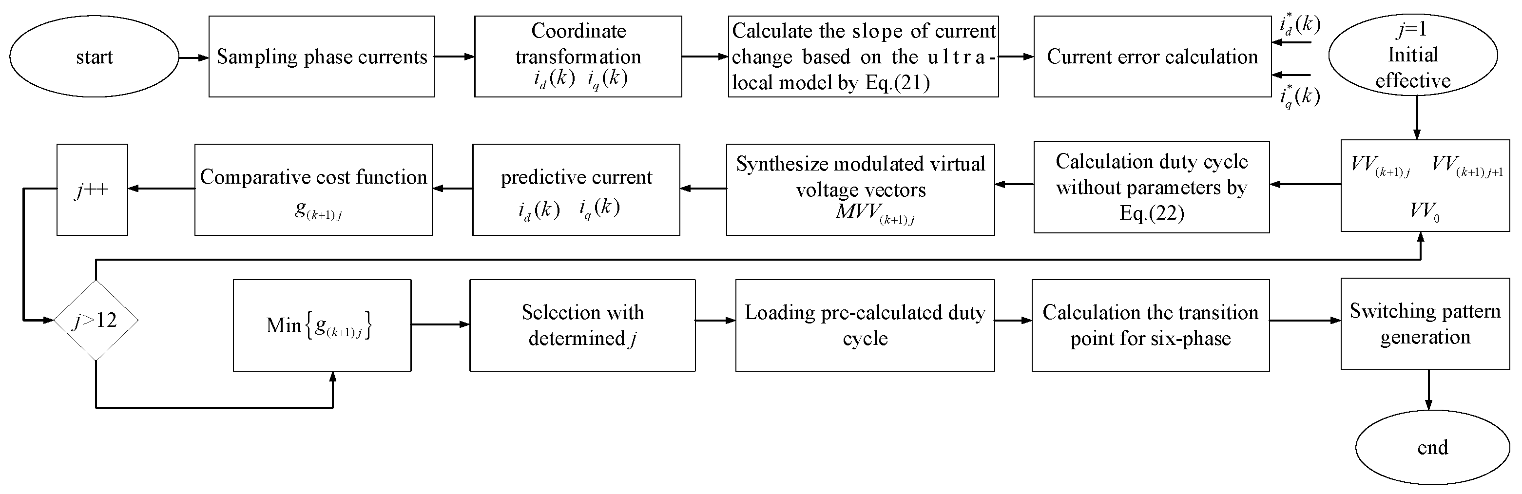
Figure 8 shows the flow diagram of the MFPCC-MVVV method.
A horizontal comparison of the five methods is given in
Table 1. As shown, both the MPCC-TARD and MFPCC-TARD methods exhibit inferior phase current quality, owing to their inability to suppress harmonic voltages in the x–y plane. Moreover, the MPCC-TARD and MPCC-VVV-TARD methods show high sensitivity to parameter variations, since their current prediction accuracy depends heavily on the precision of the motor parameters. In contrast, the latter three methods exhibit enhanced robustness to parameter mismatch by implementing an ultra-local model for current prediction. Although the MFPCC-VVV-TRAD method effectively reduces harmonic currents through virtual voltage vectors, its performance is constrained by the fixed optimal voltage vector angle and the limited accuracy of its differential-algebraic computation for nonlinear components. The proposed MFPCC-MVVV method achieves substantial improvement in current quality compared to the MFPCC-VVV-TARD method through three key innovations: first, the implementation of MVVs with variable angles and magnitudes; second, the development of a dual virtual voltage vector duty-cycle calculation without motor parameters; and third, the incorporation of an extended observer to enhance computational accuracy of nonlinear components. These advancements collectively contribute to its excellent current quality performance.
It should be noted that the main contributions of this paper are the MVVVs and the dual virtual voltage vector duty-cycle technique, which jointly extend the modulation range and significantly improve steady-state performance. In this context, the selection of an observer is intended to complement the proposed model-free predictive control framework appropriately. As summarized in
Table 2, the three observers exhibit distinct characteristics: the EKO provides optimal estimation under Gaussian noise, requires no low-pass filter, and features adaptive gains, albeit with a relatively high computational burden; the SMO offers strong robustness but suffers from inherent chattering and phase lag; the ESO is model-independent with few parameters, yet its gains are fixed and its estimation accuracy deteriorates under high noise levels. For a DT-PMSM drive system, compared with a three-phase motor, an additional harmonic plane—namely the x-y subspace—is present. This extra plane introduces additional parameters and more complex nonlinear couplings, thereby imposing higher demands on the observer’s state estimation dimensionality and parameter adaptability. The EKO, based on state augmentation and covariance recursion, can naturally extend the state variables to accommodate the extra dynamics introduced by the harmonic plane while tracking parameter variations across different subspaces via an adaptive gain matrix.
In contrast, the SMO may induce additional current ripple in the harmonic plane due to chattering, and the fixed gains of the ESO necessitate extra tuning to address the fundamental and harmonic planes simultaneously. It should be emphasized that the above analysis is not intended to claim the absolute superiority of the EKO over the SMO or ESO. Rather, it indicates that, within the proposed model-free predictive control framework for dual three-phase PMSMs, the characteristics of the EKO—adaptive gain, absence of phase lag, and capability of state augmentation—align well with the specific system requirements, namely the presence of an additional harmonic plane, multi-parameter variations, and Gaussian noise. Consequently, the EKO represents a more suitable observer choice in this context. The primary performance enhancement remains attributable to the MVVV and duty-cycle techniques. At the same time, the EKO serves as a complementary local observer that reliably estimates the nonlinear part of the ultra-local model, thereby further improving system robustness and harmonic suppression capability.
4. Experimental Verification
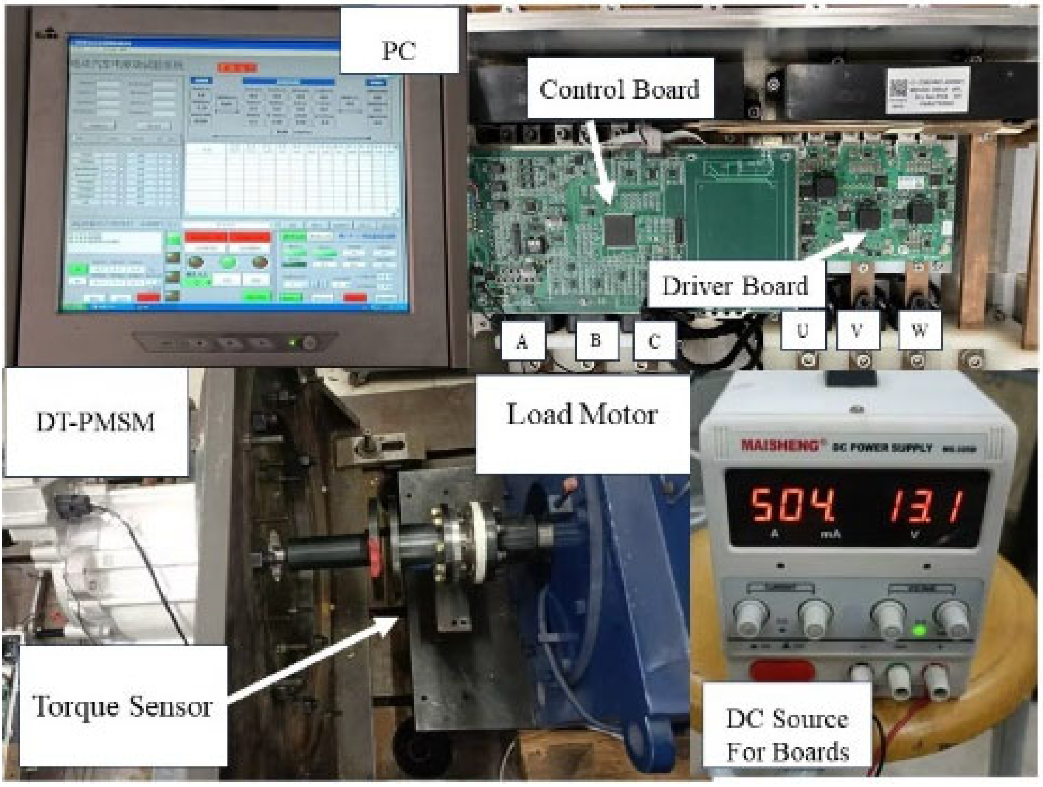
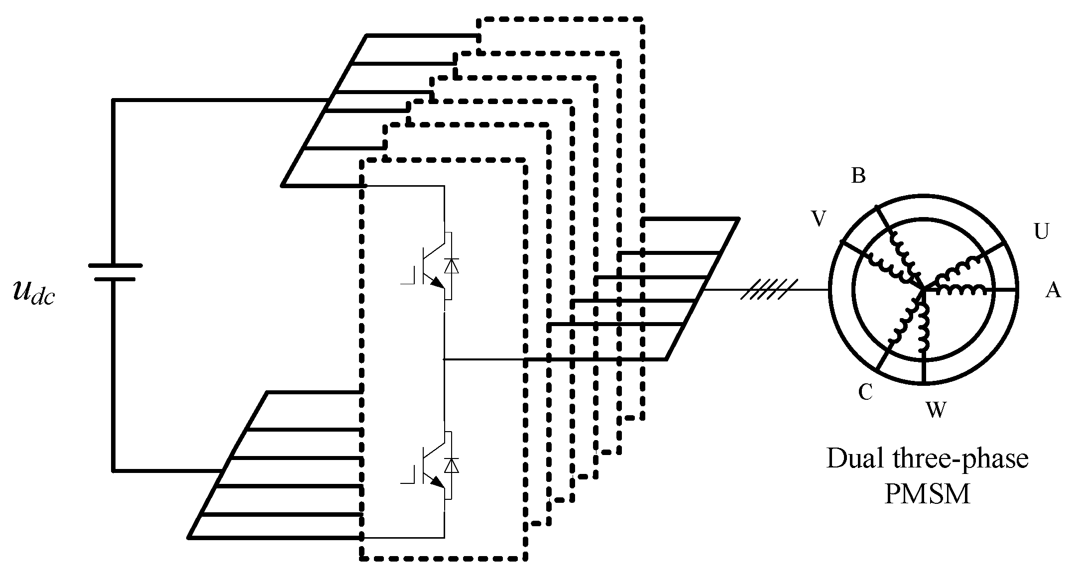
The experimental platform for model predictive control of DT-PMSM is shown in
Figure 9.
Table 3 presents the parameters of the experimental motor. The hardware system mainly consists of control circuits and power circuits. To verify the effectiveness of the proposed method, we established an experimental platform based on the TMS320F28335 microcontroller. The system features a 540 V DC bus with two equal-value series-connected capacitors to create a neutral point. A K-T40B-500Q torque sensor transmits real-time torque and speed information to the dynamometer for display, while a three-phase induction motor serves as the loading machine. This comprehensive experimental setup enables accurate performance evaluation of the proposed MFPCC-MVVV method under various operating conditions. An induction motor provides the motor load. Motor speed and torque are acquired via torque sensors, and phase currents are measured with current sensors. All acquired data waveforms are recorded and displayed on a PC. For reader convenience, the traditional model predictive control strategy based on the virtual voltage vector, as presented in Ref. [
25], is hereafter referred to as the MPCC-VVV-TARD method. The traditional MFPCC method based on virtual vector is called MFPCC-VVV-TARD method. The proposed method is called the MFPCC-MVVV method.
4.1. Steady-State Performance Under Parameter Match
Steady-state experiments were conducted under the working conditions of 1500 r/min and 6 Nm for verification. Experimental results verify the steady-state performance of the MFPCC-MVVV method under parameter-matched conditions. A comparison was made between the MFPCC-VVV-TRAD method and the proposed MFPCC-MVVV method in terms of steady-state performance under parameter matching.
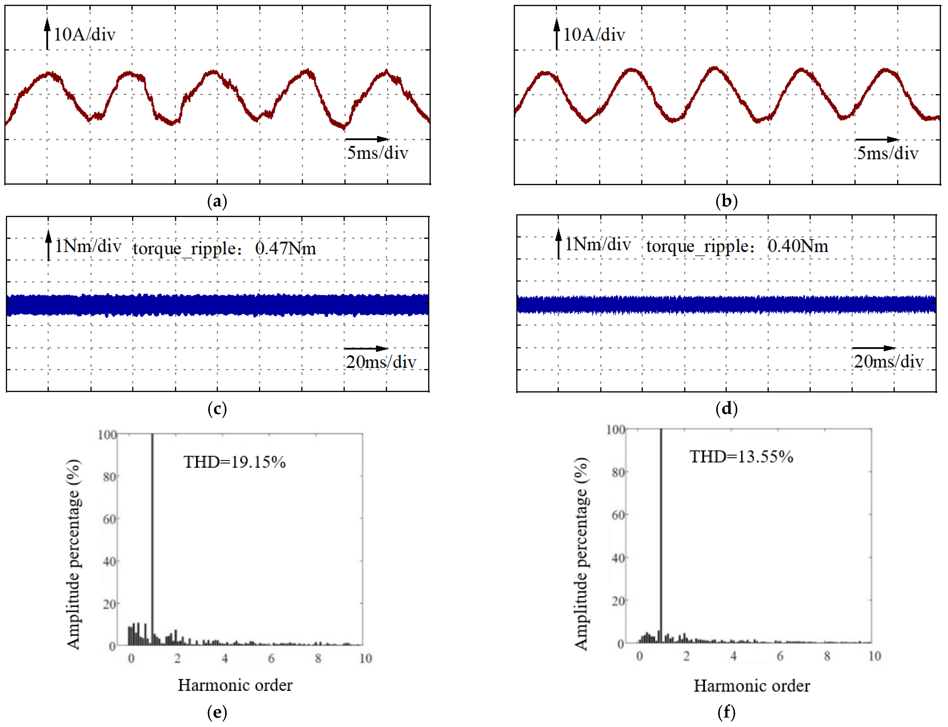
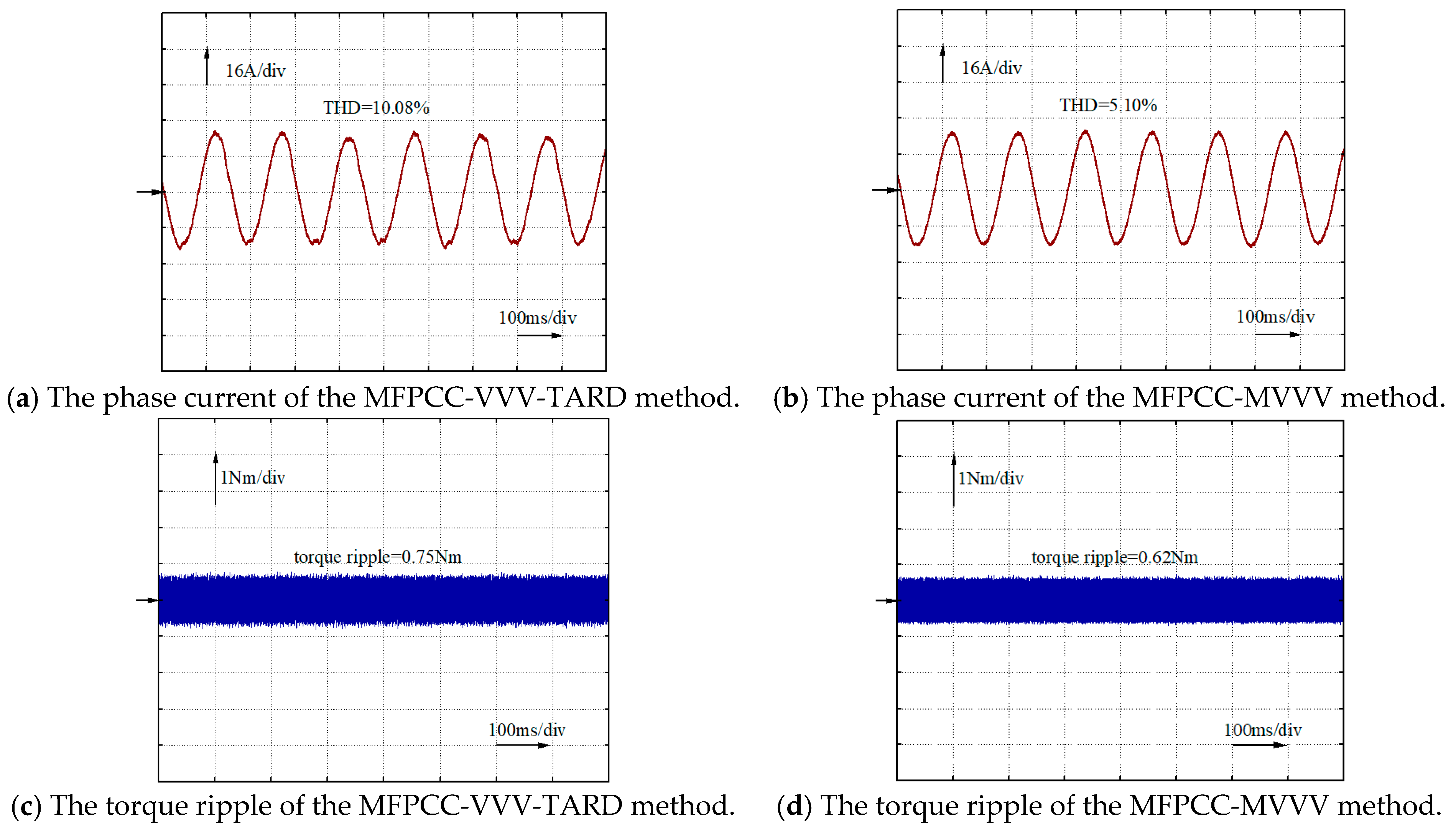
Figure 10 displays, from top to bottom, the experimental waveforms of phase current, torque, and the FFT analysis. As shown in
Figure 10a,b, the MFPCC-MVVV method employs
MVVs, significantly improving phase current quality compared to the MFPCC-VVV-TARD method. The MFPCC-MVVV method introduces MVVs, extending the modulation range to a regular dodecagon, thereby enhancing current tracking capability and achieving a more sinusoidal phase current.
Figure 10e,f present the FFT analysis of the phase current. The THD values for the phase current in MFPCC-VVV-TARD method and the MFPCC-MVVV method are 19.15% and 13.55%, respectively, demonstrating the superior phase current quality of the MFPCC-MVVV method. Furthermore, torque ripple was analyzed for both methods.
Figure 10c,d reveal that the MFPCC-MVVV method generates significantly lower torque ripple compared to MFPCC-VVV-TARD method, reducing it to 0.40 Nm.
To verify the effectiveness of the proposed method under low-speed operating conditions, experiments were conducted at 100 r/min and a load torque of 6 Nm.
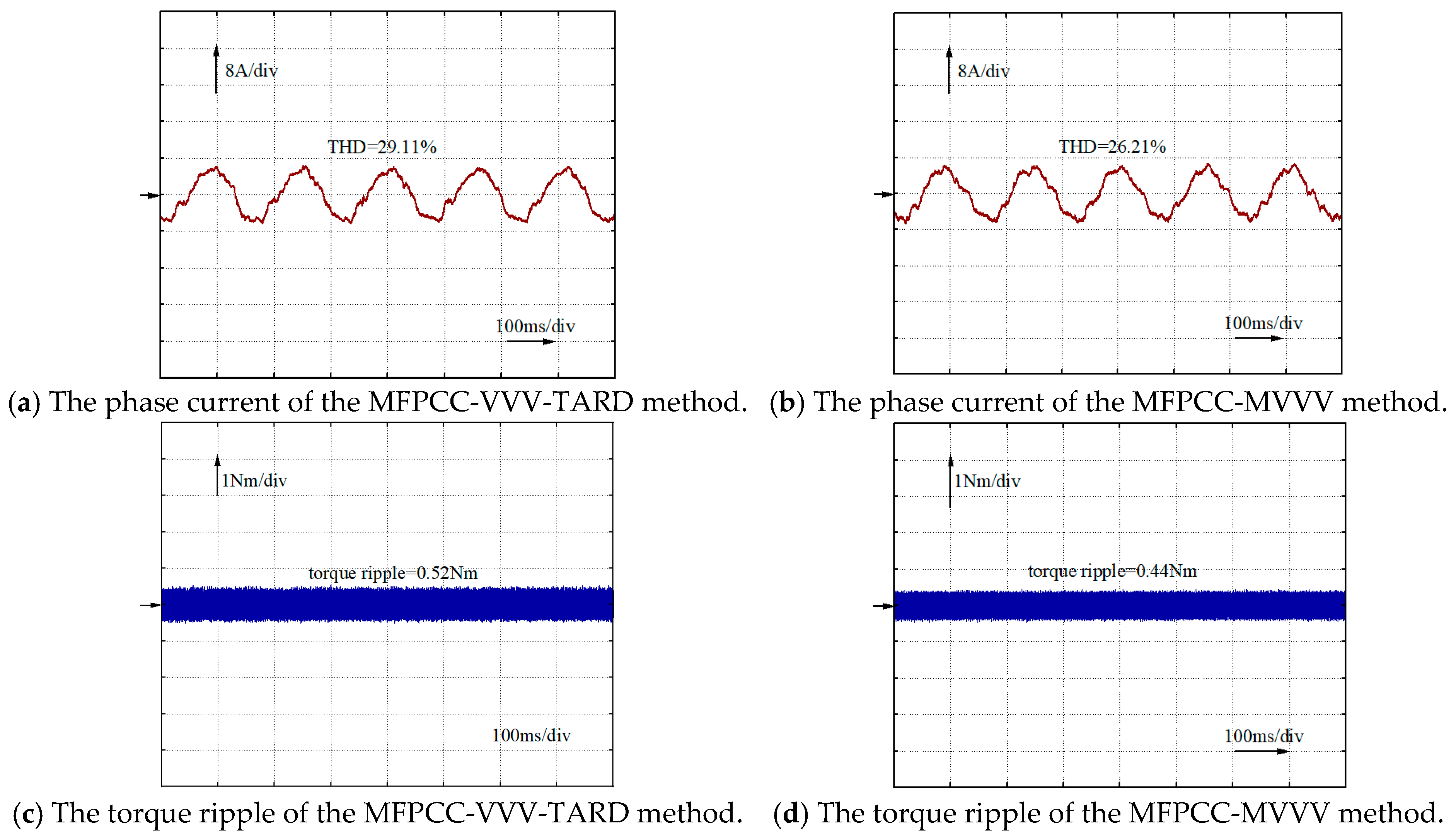
Figure 11 presents the experimental waveforms of both methods during low-speed operation. It can be observed from the figure that, compared with the medium-speed and medium-load condition, both methods exhibit increased phase current distortion at low speed, primarily due to inverter nonlinearity-induced voltage distortion and the very short duration of the zero-vector action. These factors lead, on one hand, to a significant increase in the THD of the current, and on the other hand, to an increase in torque ripple amplitude due to the interaction between harmonic currents and the fundamental magnetic field. Nevertheless, the proposed method outperforms the conventional method in terms of both current THD and torque ripple.
Figure 12 shows the experimental results of the two methods under the condition of 1500 r/min and a load torque of 28 Nm. Compared with the medium-speed and medium-load conditions, the phase current THD of both methods decreases under this operating point. The main reason is the substantial increase in load current, which significantly raises the fundamental amplitude. In contrast, the harmonic currents increase only moderately owing to non-ideal factors such as dead-time effects. Consequently, the harmonic proportion relative to the fundamental is reduced.
On the other hand, because the absolute amplitude of harmonic currents increases with load, the absolute torque ripple becomes larger. Despite this trend, the proposed method still achieves lower phase current THD and smaller torque ripple than the conventional method, further validating its effectiveness. In summary, experimental comparisons confirm that the MFPCC-MVVV method delivers superior steady-state performance when motor parameters are matched.
4.2. Dynamic-State Performance Under Parameter Match
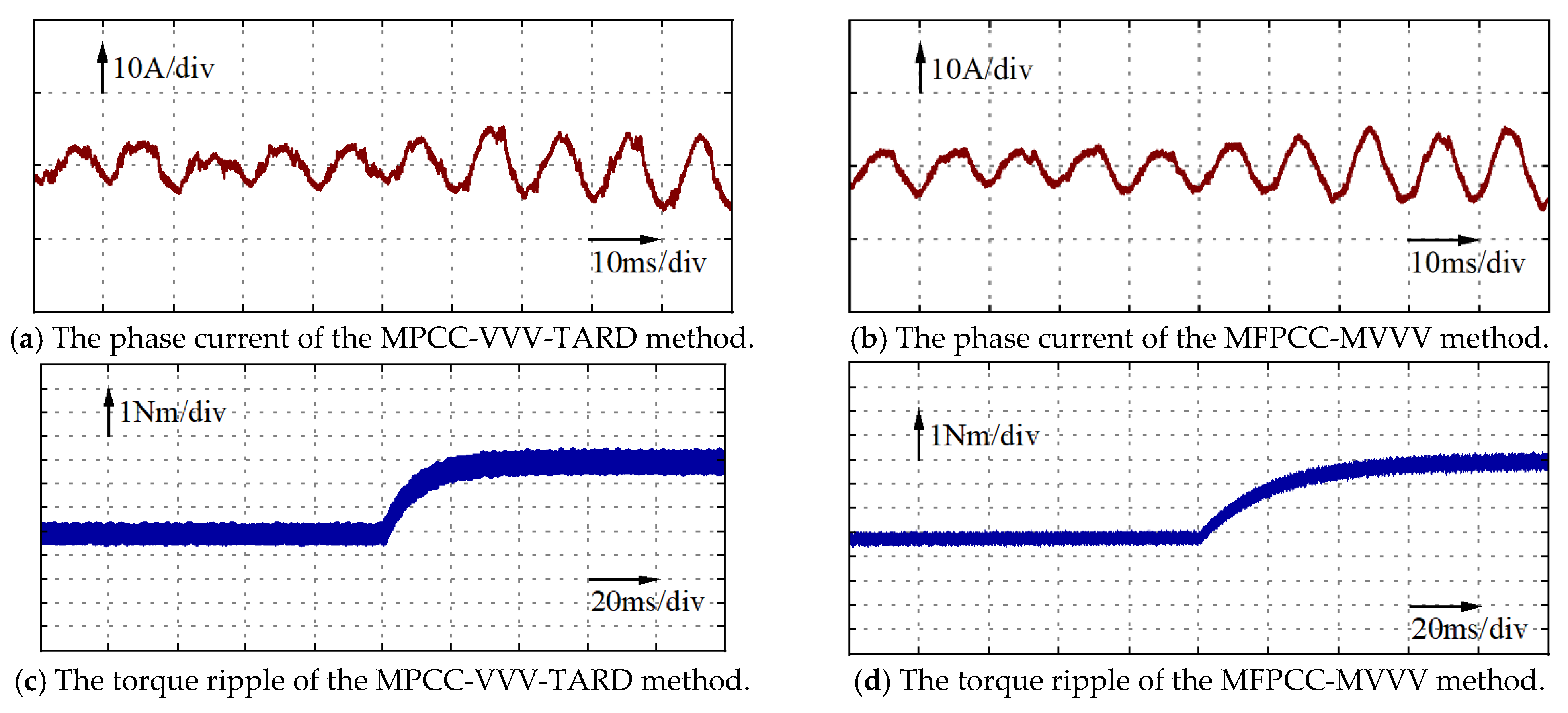
Figure 13 presents a comparative analysis of the dynamic performance of the MFPCC-VVV-TARD method and the proposed MFPCC-MVVV method using experimental waveforms. Under a speed condition of 1500 r/min with a sudden load increase from 3 Nm to 6 Nm, both methods demonstrate effective torque tracking capability with comparable response times when motor parameters are matched, confirming the excellent dynamic response of the MFPCC-MVVV method. Furthermore, the MFPCC-MVVV method maintains its superior performance in terms of phase current quality and reduced torque ripple, thereby validating the effectiveness of the proposed method.
4.3. Steady-State Performance Under Parameter Mismatch
Steady-state performance under parameter-mismatch conditions was tested at 1500 r/min with a 6 Nm load.
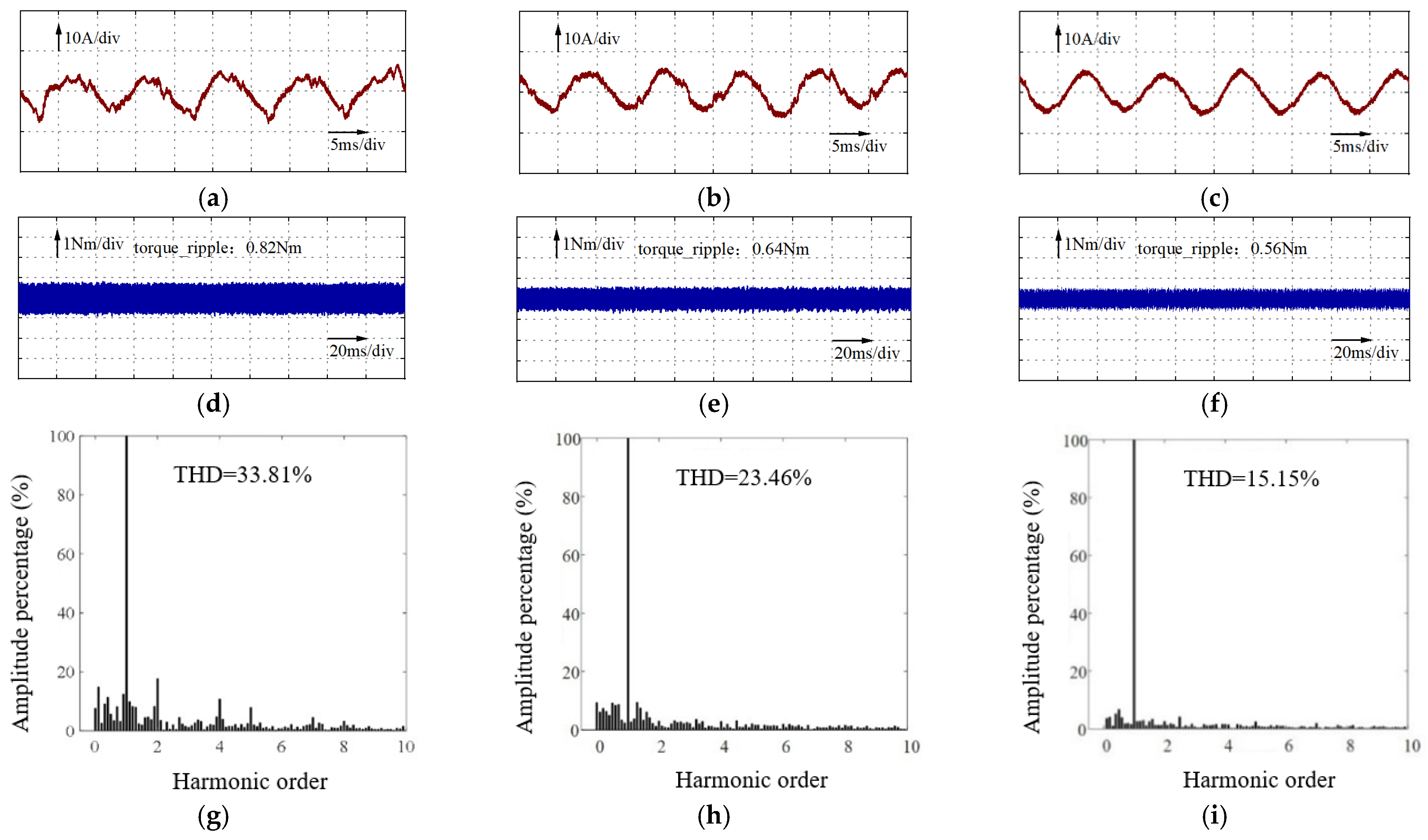
Figure 14 presents the phase current waveforms, torque waveforms, and FFT analysis for three methods: the MPCC-VVV-TARD, the MPCC-VVV-TARD, and the proposed MFPCC-MVVV method. The motor parameters were mismatched as follows:
Rs = 0.5
Rs0,
Ld = 0.5
Ld0,
Lq = 0.5
Lq0, and
ψf = 1.2
ψf0, where
Rs,
Ld,
Lq, and
ψf represent actual values while
Rs0,
Ld0,
Lq0, and
ψf0 denote nominal values. Analysis of
Figure 14a–c reveals that reduced motor inductance altered the
q-axis reference current tracking, increasing phase current THD for all three methods compared to parameter-matched conditions. The MPCC-VVV-TARD method exhibited particularly severe current performance degradation, as both its duty-cycle calculation and predictive model heavily depend on motor parameters, making optimal voltage vector selection highly sensitive to inductance variations. FFT analysis in
Figure 14g–i shows the Ref. MPCC-VVV-TARD method THD reached 33.81% under parameter mismatch. In contrast, both the MPCC-VVV-TARD method and the MFPCC-MVVV method demonstrated better robustness, with THD values of 23.46% and 15.15%, respectively. This improvement stems from two key factors: (1) the ultra-local model’s inherent parameter robustness, and (2) for the MFPCC-MVVV method specifically, the expanded modulation range through
MVVs and optimized current change rate/duty-cycle calculations via the ultra-local model. Torque ripple analysis in
Figure 14d–f further confirms the proposed method’s superiority, showing values of 0.82 Nm, 0.64 Nm, and 0.56 Nm for the MPCC-VVV-TARD, MFPCC-VVV-TARD, and MFPCC-MVVV methods, respectively.
Table 4 presents the experimental results of the three methods under various motor parameter mismatches.
Table 4 shows that, under parameter mismatches, the proposed method achieves the best steady-state performance among the three methods, demonstrating its effectiveness. Furthermore, inductance parameter mismatch has the greatest influence on steady-state performance. These experimental results conclusively demonstrate that the MFPCC-MVVV method maintains excellent steady-state performance while exhibiting strong robustness against parameter mismatches.
4.4. Dynamic-State Performance Under Parameter Mismatch
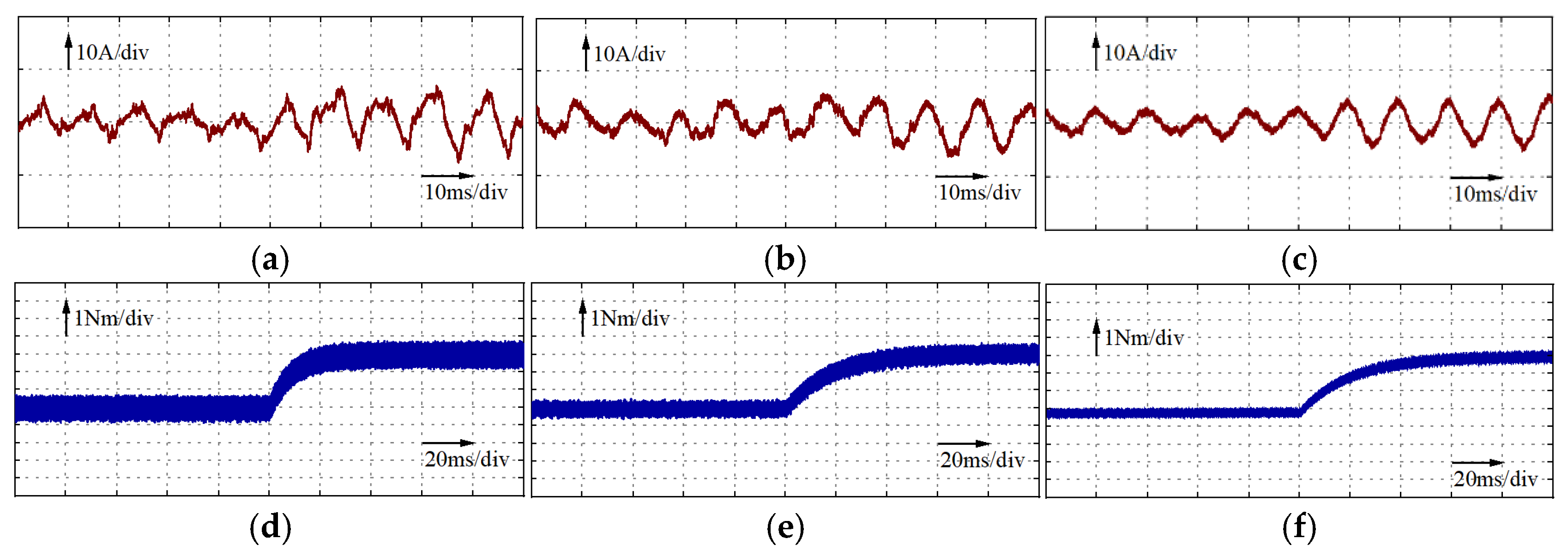
The dynamic performance of three methods under parameter mismatch conditions was experimentally investigated at 1500 r/min with a sudden load step change from 3 Nm to 6 Nm. As shown in
Figure 15, which displays the dynamic responses from left to right for each method, the MPCC-VVV-TARD method exhibited significant performance degradation due to its parameter-dependent predictive model and duty-cycle calculation, leading to suboptimal voltage vector selection, inaccurate current prediction, severe phase current distortion, and increased torque ripple. In contrast, the proposed MFPCC-MVVV method demonstrated superior performance, maintaining better phase current quality than the MPCC-VVV-TARD method both before and after the load change, with smooth current transitions and rapid torque response that effectively tracked the reference value. These experimental results confirm the excellent dynamic performance of the MFPCC-MVVV method under parameter-mismatch conditions, which is fully consistent with the theoretical conclusions. The robustness of the MFPCC-MVVV method stems from its reduced parameter sensitivity and optimized control algorithm.
4.5. Computational Burden Test
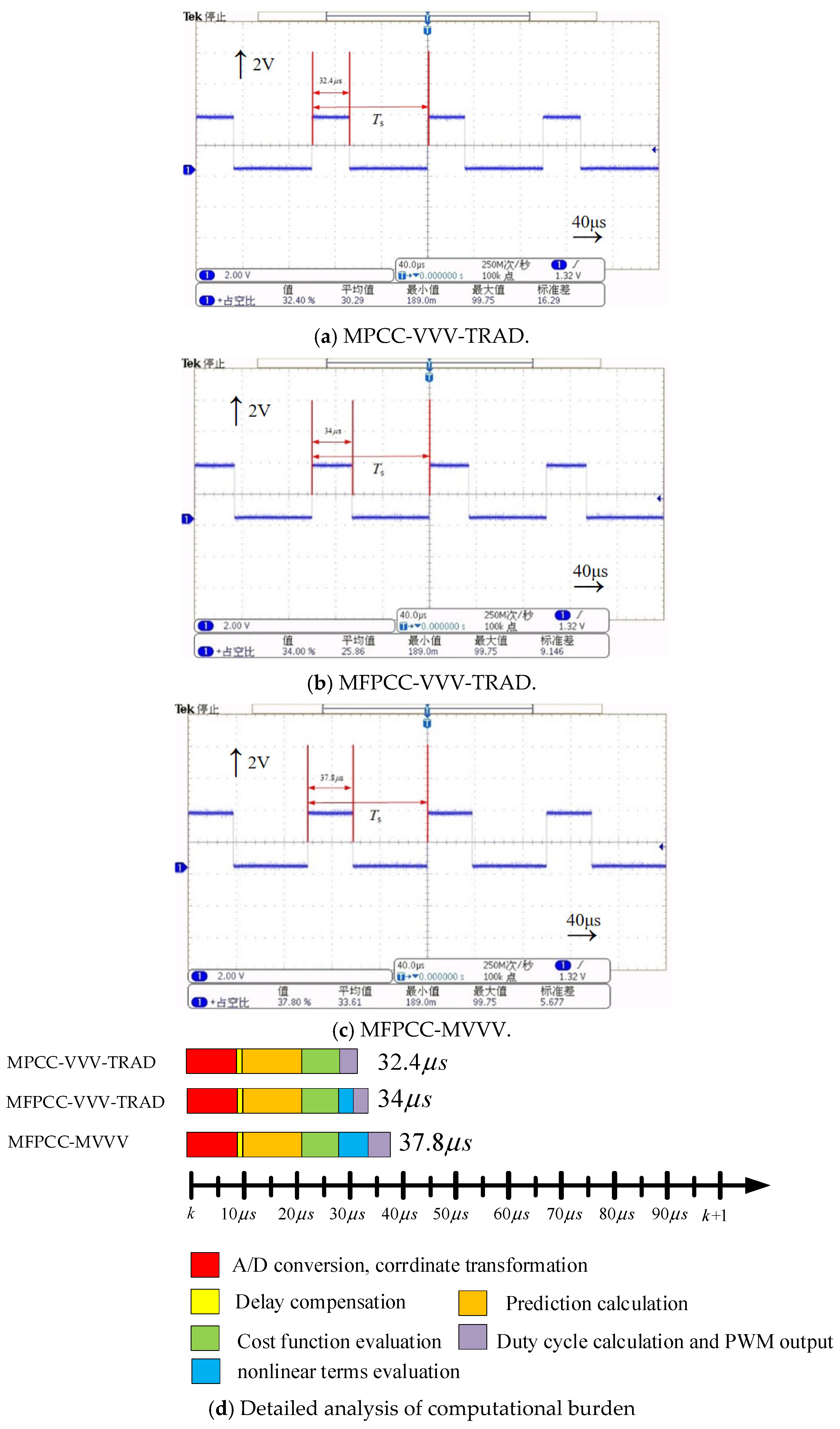
Figure 16 compares the computational burden of the three methods. The execution times are measured using the digital signal processor’s GPIO toggling method: a high level is output while the respective algorithm is executing. As shown in
Figure 16a–c, the total computational burdens of MPCC-VVV-TRAD, the MFPCC-VVV-TRAD method, and the proposed MFPCC-MVVV method are 32.4 μs, 34.0 μs, and 37.8 μs, respectively.
Figure 16d further presents the detailed execution times for each functional module across all three methods. In comparison with MPCC-VVV-TRAD, the MFPCC-VVV-TRAD method introduces an ultra-local model prediction, increasing the computational burden by 1.6 μs. The proposed method employs an EKO to estimate the nonlinear disturbance terms, which involves calculations such as the Jacobian, covariance, and Kalman gain matrices; consequently, its computational burden increases by an additional 3.8 μs relative to the conventional method.
Nevertheless, the total execution time of the proposed method remains below 50 μs, which is well below the 100 μs control period. This leaves more than 60 μs of idle time for other interrupt-handling tasks or communication, thereby ensuring the reliable operation of the real-time control system. Moreover, the increase in resource occupancy on the digital signal processor is modest, imposing no significant additional computational burden. These results demonstrate the good engineering feasibility of the proposed method on low-cost processors such as the TMS320F28335.
5. Conclusions
This paper proposes an MFPCC-MVVV based on an EKO and MVV for DT-PMSM. By establishing an ultra-local model, the method eliminates dependence on motor physical parameters. The EKO is employed to estimate the nonlinear disturbance terms, thereby improving model accuracy. The MVV achieves continuous modulation and expands the voltage modulation range. Combined with a parameter-free duty-cycle calculation and a triangular-carrier-based asymmetric PWM generation strategy, the proposed method offers high robustness, low current ripple, and ease of implementation on low-cost processors.
Experimental results demonstrate that under parameter-matched conditions (1500 r/min, 6 Nm), the proposed method achieves a phase current THD of 13.55% and a torque ripple of 0.40 Nm, outperforming the conventional method (19.15% and 0.64 Nm, respectively). Under parameter-mismatched conditions, the proposed method maintains a THD of 15.15% and a torque ripple of 0.56 Nm, whereas the conventional method degrades to 33.81% and 0.82 Nm. The computational burden is only 37.8 μs, confirming its superior steady-state performance, robustness, and engineering feasibility.
We should note three limitations: (a) the scaling factors and are tuned by empirical trial-and-error; (b) the method has been validated only on dual three-phase PMSMs, not yet extended to induction motors nor investigated under fault-tolerant operating conditions; (c) the tuning of the EKO covariance matrices still requires empirical adjustments. Future research will focus on: (a) online learning-based automatic tuning of the scaling factors; (b) extension of the method to induction motors and investigation of its fault-tolerant capability under open-circuit faults; and (c) integration with model predictive torque control. This work lays a solid foundation for high-performance model-free predictive control of multiphase motor drives.