Article

Polarization Recovery-Based Screening of Lithium-Ion Cells After Pulse Multisine Loading

Audi Hungaria Faculty of Automotive Engineering, Széchenyi István University, 9026 Győr, Hungary
Electronics 2026, 15(11), 2291; https://doi.org/10.3390/electronics15112291
Submission received: 27 April 2026 / Revised: 16 May 2026 / Accepted: 18 May 2026 / Published: 25 May 2026

Abstract

Fast and scalable lithium-ion cell diagnostics require measurements that are shorter and simpler than full impedance analysis, yet richer and more interpretable than single scalar resistance indicators or raw waveform classification alone. This paper introduces a practical recovery stamp screening method in which short post-load voltage recovery intervals after pulse and pulse–multisine excitation are treated as compact diagnostic events, rather than as single resistance-like indices or parameter identification segments. For this purpose, a constrained two-timescale relaxation model is introduced to retain fast and slower recovery contributions in a low-dimensional form. Using laboratory measurements on two lithium-ion pouch cell families based on nickel manganese cobalt oxide (NMC)/graphite and LiFePO4/graphite chemistry, each retained load removal event is converted into a signed, current-normalized recovery curve and parameterized by the proposed model. The fitted parameters provide a compact, physics-informed recovery state, while the resampled local waveform preserves transition morphology and short-time relaxation structure that are not fully retained by compact variables alone. These two inputs are evaluated separately and jointly in ordered event sequences under a reference-centered binary screening formulation. The curated dataset comprises 48 original recovery events. Local label-preserving augmentation is applied as training-side regularization, yielding 490 event instances and 230 event sequences. A scalar recovery-amplitude baseline has reached balanced accuracies of 0.833 without and 0.929 with operating context, whereas the best deep learning result is obtained only when fitted variables and waveform are combined. In that setting, TimesNet has reached a median validation balanced accuracy of 0.938. These findings show that post-load polarization recovery contains diagnostically useful information beyond scalar amplitude measures and can support rapid, interpretable reference-deviation screening.

1. Introduction

In recent years, lithium-ion batteries have become the dominant energy storage technology in electric vehicles (EVs) and in a growing range of stationary applications. At the same time, the increasing deployment of these systems has made early fault detection a matter of both safety and reliability. In this context, the timely detection of abnormal cell behavior is particularly important because battery faults may evolve gradually, remain weakly observable in their early stage, and yet eventually lead to severe degradation or safety-critical events [1,2,3].
A considerable amount of research has therefore been devoted to battery fault diagnosis. Existing approaches may be broadly divided into model-based, signal-processing-based, and data-driven methods [1,2,3]. Data-driven methods, in particular, have attracted growing attention because they can exploit large volumes of voltage, current, and temperature data without requiring a complete first-principle description of the cell. Recent studies have adopted for instance segmented regression [4], spatio-temporal transformer networks [5], dynamical deep learning [6], and model-constrained deep learning [7] for battery fault detection or prognosis under increasingly complex operating conditions. These studies clearly indicate that artificial intelligence (AI)-based diagnosis is becoming a major research direction.
The previous literature has established that pulse–multisine excitation carries richer dynamic information than conventional Hybrid Pulse Power Characterization (HPPC)/Pulse Power Characterization (PPC)-based parametrization. In particular, the signal-design study of Widanage et al. has shown that PPC data may lead to modeling error when parametrization is performed over a narrower bandwidth than that encountered under drive-cycle-like operation, whereas pulse–multisine excitation provides a profile with broader amplitude and frequency content and is therefore more representative of practical dynamic loading [8]. The same study has further shown that the required experimental time can be reduced from several hours to several minutes per state-of-charge and temperature point while maintaining modeling relevance in the bandwidth of interest for battery management applications [8]. In addition, the model-estimation study of Widanage et al. has shown that the increased bandwidth and the high number of signal levels of a pulse–multisine input support the characterization of battery dynamics and nonlinear effects without requiring a full three-dimensional lookup-table parametrization [9].
Electrochemical impedance spectroscopy (EIS) remains uniquely powerful for separating processes associated with different relaxation times. However, this separation requires a sufficiently small perturbation around a nearly stationary operating point, so that state of charge (SOC), temperature, and polarization drift do not change appreciably during the measurement [10]. Moreover, the recent review of Nováková et al. has emphasized that the conventional single-sine method is still the most accurate form of EIS measurement, yet remains too slow for online battery diagnostics in a battery management system (BMS) [11].
These measurement-related limitations are closely connected to the machine learning (ML) formulation itself. For safety-critical battery applications, physically interpretable inputs are preferable to purely opaque waveform-based decisions, which is consistent with the review of Faraji Niri et al. on explainable machine learning for lithium-ion batteries [12]. At the same time, different battery faults are often difficult to diagnose and isolate because of their similar features and internal coupling relationships [3]. Consequently, under comparable operating conditions, systematic separation from a designated family-specific reference may provide a more realistic screening target than direct fault-mechanism identification.
However, despite this progress, two issues remain open. First, many existing methods rely either on raw operational data streams or on scalar indicators that are only indirectly related to the underlying electrochemical dynamics. Second, as pointed out in recent reviews, there is still a gap between high-performing laboratory diagnosis methods and robust real-world deployment, mainly because of domain shift, heterogeneous operating conditions, and the limited availability of well-labeled fault data [2,3]. In practice, the difficulty is therefore not only the selection of the learning model, but also the form of the information supplied to it. Cell-level fault labels are expensive and often incomplete, while long impedance or pulse-test procedures are not always compatible with rapid screening. This creates a need for intermediate representations that are short to measure, physically interpretable, and informative for AI-based discrimination.
In parallel with the development of AI-based diagnosis, pulse- and recovery-based battery characterization has shown that short transient responses can reveal useful information on polarization-related internal dynamics. Hao et al. [13] demonstrated that pulse-response functions can be used to describe battery polarization and support state estimation using short relaxation intervals. Likewise, rapid pulse-based studies have shown that dynamically excited voltage responses can provide diagnostically relevant information beyond conventional scalar tests, especially when the excitation is made richer and more structured [14]. These observations suggest that short post-excitation recovery segments may contain fault-related information that is not fully captured by conventional state variables such as capacity fade or single-point resistance measures. LiFePO4-based cells are particularly relevant for recovery-oriented transient diagnostics because their electrochemical behavior is strongly influenced by lithium-ion transport limitations, diffusion-controlled relaxation processes, crystallinity, and phase-purity-dependent polarization dynamics [15].
Motivated by the above considerations, this paper introduces a new intermediate recovery stamp representation for reference-centered state-deviation screening in lithium-ion cells. The retained recovery events are acquired at 10 kHz to preserve the immediate post-switching voltage step, early relaxation morphology, and short-time recovery structure. Compact-variable, waveform-only, and combined input settings are evaluated on the curated corpus using neural sequence models and a non-temporal dense baseline. The final combined input comparison contrasts TimesNet [16] with GRU and multilayer perceptron (MLP) alternatives, and tests whether period-aware temporal mixing can exploit recovery-waveform morphology together with physically interpretable compact variables. Compared with pulse-resistance indices and recovery models aimed mainly at parameter identification or state estimation, the proposed method uses each load removal interval as a normalized diagnostic event. The measured recovery is mapped to a signed current-normalized stamp, then represented by a compact two-timescale recovery state and a fixed-length local waveform. The ordered event sequence is evaluated relative to a family-specific reference, so that degradation-related polarization deviation can be inferred from systematic separation from the reference behavior.

2. Measurement Setup and Data Acquisition

2.1. Diagnostic Measurement System

According to actual industrial practice, pulse-series testing, in particular HPPC [17], is among the most frequently adopted excitation methods for lithium-ion (Li-ion) batteries when identifying the parameters of equivalent-circuit models (ECMs). However, this approach has several limitations. In particular, it does not reproduce the strongly dynamic operating conditions encountered in real vehicle applications. Consequently, datasets generated in this way contain only limited information on the actual dynamic behavior of the cell under practical usage patterns and/or driving conditions [18]. Standard driving cycle current profiles have also become widely used (see, e.g., [19,20]). Such profiles are more dynamic than PPC-type tests in terms of amplitude variation and frequency content; nevertheless, an excitation strategy that ensures sufficient generality while simultaneously reducing modeling error is still required.
Standardized procedures for lithium-ion traction-battery testing are available in the International Organization for Standardization (ISO) 12405 and International Electrotechnical Commission (IEC) 62660 standard families. At pack and system level, ISO 12405-4:2018 specifies performance testing for lithium-ion traction battery packs and systems and replaces the earlier high-power and high-energy application parts, ISO 12405-1:2011 and ISO 12405-2:2012. At the cell level, IEC 62660-1:2018 specifies performance and life testing, IEC 62660-2:2018 addresses reliability and abuse testing, and IEC 62660-3:2022 specifies safety requirements for secondary lithium-ion cells and cell blocks used for electric road-vehicle propulsion [21,22,23,24]. At the same time, multisine signals are widely used in engineering practice for application-oriented experiment design and for characterizing nonlinear systems in the frequency domain, because their spectral lines, amplitudes, and phases can be prescribed directly (see, e.g., [25]). On this basis, the multisine approach is considered suitable for generating measurement datasets that contain information on nonlinear cell dynamics, including terminal voltage and calculated state-of-charge, under dynamically varying load profiles. In particular, multisine excitation can be configured so that it is statistically similar to the alternating discharge and regenerative-braking events experienced by a cell in vehicle operation. Compared with the waveforms prescribed in standardized procedures, multisine excitation offers broader and more flexible amplitude and frequency content and therefore approximates real driving conditions more closely.
An additional advantage of random-phase multisine charge/discharge signals in automotive battery diagnostics is that the waveform can be adjusted to the characteristics of the given cell type. In contrast to standardized vehicle-level driving cycles, such as the Worldwide Harmonized Light Vehicles Test Procedure (WLTP), which define fixed speed–time trajectories rather than a unique cell-level current waveform, random-phase multisine charge/discharge signals can be applied at arbitrary initial cell voltage and to cells in different conditions, including degraded and deeply discharged states. Moreover, such excitation may improve modeling accuracy while reducing the required measurement time to a few minutes per charge level and temperature, in contrast to the several hours often required for PPC-based measurement series.
A multisine-based test procedure representing the effects of the dynamic loads occurring in real vehicle applications is therefore required. Such multisine approaches have been introduced for lithium-based battery testing mainly in connection with equivalent-circuit or EIS-related modeling [8,26], or for SOC estimation [27]. However, the diagnostic use of such signals for fault-related transient feature extraction from lithium-ion cells has not been the primary focus of those studies.
For this reason, the experiments reported in this paper are conducted on a dedicated lithium-ion cell diagnostic measurement system [28] that supports automated multicell testing, programmable loading, synchronized data acquisition, and external waveform-driven excitation. The system supports conventional pulse/spot measurements, stress vector-driven test execution, and externally programmed waveform-defined loading profiles, including random-phase multisine excitation. This capability makes it possible to realize both controlled and realistic transient operating scenarios and, consequently, to generate datasets containing information over a broad portion of the dynamic range of the cell or cell pack, including transient fault-related signatures.
The apparatus [28] is based on a National Instruments cDAQ9188 data-acquisition platform. The setup includes an NI-9472 digital output module for shift-register gating, a custom switching matrix for automated cell selection, and an NI-9263 analog output module that provides the external programming signal for the (Hewlett-Packard) HP 6050A electronic load mainframe direct-current (DC) electronic load, thereby enabling the generation of various excitation patterns. The electronic load supports external analog programming with an approximate 10 kHz ( 3 dB) bandwidth in constant-current mode. Current measurement is performed by means of a calibrated precision shunt resistor inserted in the load path. The terminal voltages of the connected cells are acquired by an NI-9206 analog input module with a 16-bit multiplexed analog-to-digital converter (ADC) front end [29,30]. All modules are configurable in the executable driver. The patented measurement system and its custom in-house LabVIEW-based measurement and control software, developed using NI LabVIEW 2018 (National Instruments, Austin, TX, USA), support both manual and automated operation, and the individual test modes are defined by test vectors. The front panel of the main virtual instrument (VI) is shown in Figure 1.
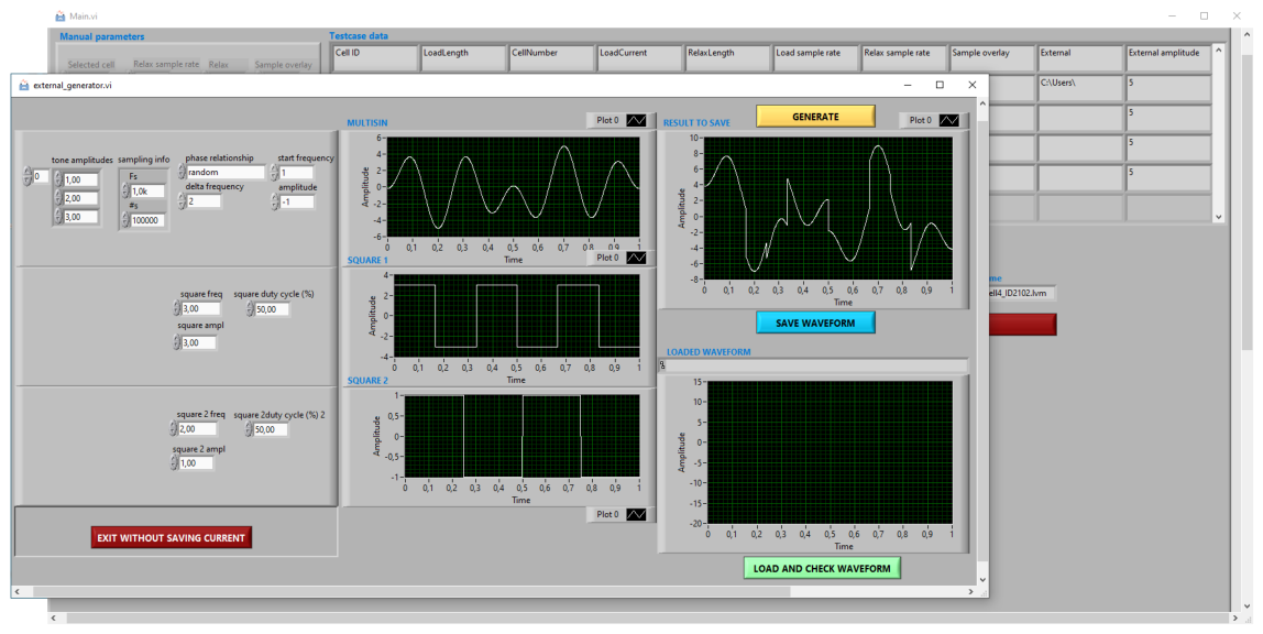
The excitation waveform can be configured in the External Signal Tool of the software, as shown in Figure 2. This tool enables flexible generation and adjustment of user-defined excitation signals. Within the present system architecture, three practically relevant excitation realizations are considered. The first consists of manual pulse-train (PT) measurements, which serve as short, controlled transient measurements. The second is the stepped pulse-train branch of the Stress mode, which corresponds to a vector-defined sequence of load and relaxation events and therefore represents an automated pulse-series experiment. The third consists of waveform-defined Stress records, including random-phase multisine and pulse-train multisine external-signal excitation. The purpose of this measurement strategy is to expose both fast and slow recovery dynamics within short post-excitation windows while retaining compatibility with practically relevant diagnostic test procedures.

2.2. Test Protocols and Measurement Data

Two operating modes are considered in the present study. In the manual mode, the operator specifies a single event by defining the selected cell, the target current, the load duration, the relaxation duration, and the corresponding sampling settings. In the stress mode, the experiment is executed automatically from a tabulated test vector. Each row of the vector defines one commanded event and contains the mandatory fields Cell ID, Cell number, Load current, Load length, Relax length, and the corresponding sampling parameters. In addition, the stress-vector format supports the optional fields External waveform, External amplitude, and Pure load. Consequently, externally programmed waveform-defined excitations, including random-phase multisine and pulse-train multisine variants, constitute realizations of the stress measurement type.
The stepped pulse-train branch of the stress protocol follows the short-pulse HPPC-type characterization [17]. The present implementation does not reproduce the standardized HPPC sequence in full. The objective here is not power-capability rating, but the controlled excitation of voltage transients followed by diagnostically interpretable recovery intervals. For this reason, lower current amplitudes are prescribed than in classical high-power HPPC practice, and the test-vector rows are configured such that post-excitation recovery remains observable without excessive overlap between consecutive events. In the waveform-defined stress records, the same row-based execution logic remains in effect, while the instantaneous current is modulated by the externally synthesized signal. When Pure load is enabled, load-only modulation is imposed; otherwise, the applied waveform may generate alternating charge/discharge operation around the selected current offset.
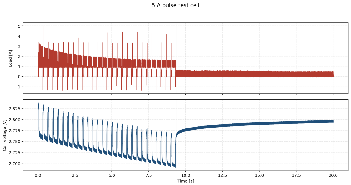
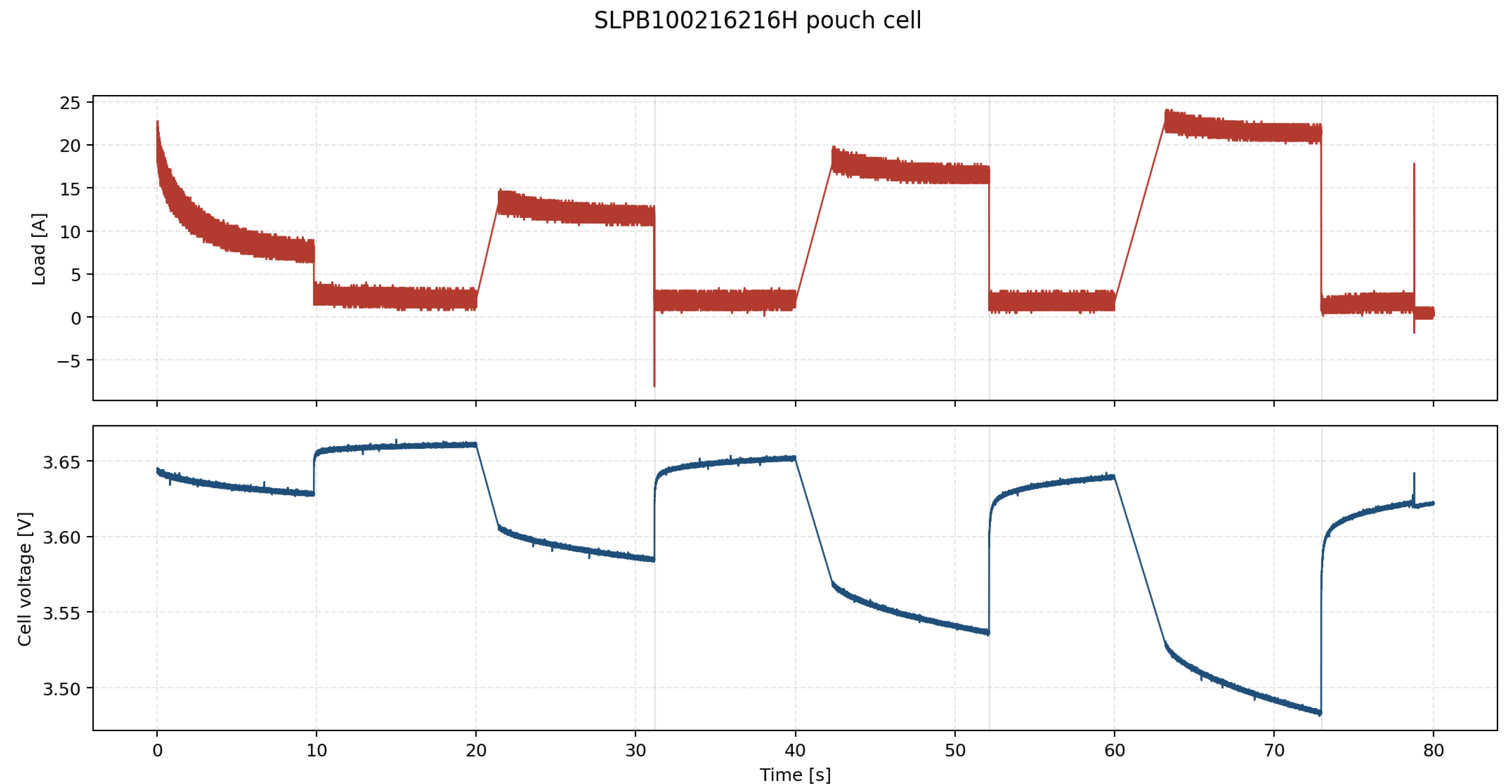
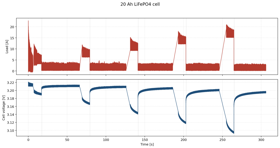
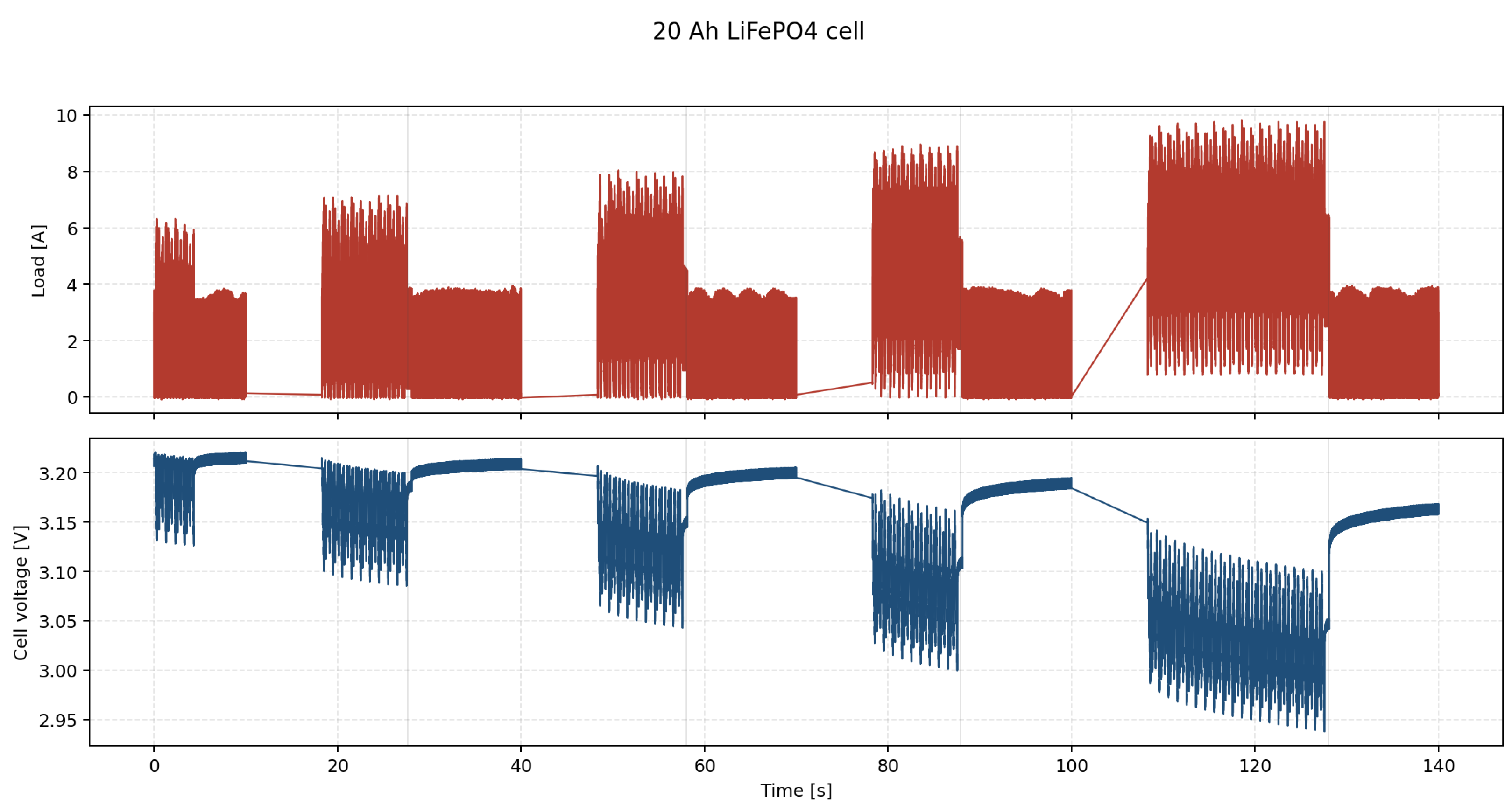
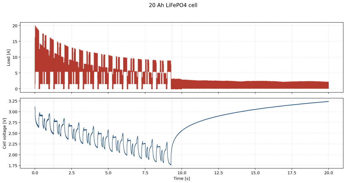
Figure 3, Figure 4, Figure 5, Figure 6 and Figure 7 present representative raw measurements from the practically relevant excitation classes used in the present work. Figure 3 presents a low-voltage 5 A manual pulse-train record sample. Figure 4 displays a higher-amplitude manual pulse-train record of the 40 Ah pouch cell family, representative of the manually prescribed increasing 10, 15, 20 A , and 25 A loading regime. Figure 5 presents a stepped pulse-train stress record of the 20 Ah LiFePO4 family with clearly separated recovery intervals. Figure 6 displays a waveform-defined stress record in which a random-phase multisine component is superposed on successive current plateaus. In Figure 7, a waveform-defined stress record with a pulse-train multisine external signal on a deeply discharged, non-reference 20 Ah LiFePO4 pouch cell can be seen.
Only the informative windows that contain the commanded excitation block and the subsequently retained recovery segments are shown. Longer pre-event or post-event baseline stretches are intentionally omitted because they contribute little to event-level discrimination. The different time axes therefore reflect the different command structures of the measurements. In particular, the manual pulse-train and stepped stress pulse-train records are organized around 10 s pulse segments, whereas the waveform-defined multisine and pulse-train multisine external-signal records use protocol-specific excitation windows and recovery durations.
All retained measurement records are acquired at 10 kHz , which corresponds to a sampling interval of Δ t = 100 μ s . This sampling interval determines how much of the early current-interruption recovery remains observable before the first recorded sample. The calculation uses the single-mode exponential relaxation term underlying the recovery model, which is defined in Section 3.2, where the post-interruption response follows from first-order polarization branches in equivalent-circuit battery models [13,18]. For one mode with initial amplitude a i and time constant τ i , the normalized fraction that has already evolved before the first recorded sample is
ε i ( Δ t , τ i ) = a i a i exp ( Δ t / τ i ) a i = 1 exp ( Δ t / τ i ) .
For Δ t = 100 μ s , Equation (1) gives first-sample losses of 9.5 % , 4.9 % , and 1.0 % for τ i = 1 , 2, and 10 ms , respectively. At 1 kHz , the corresponding losses are 63.2 % , 39.3 % , and 9.5 % . The selected sampling interval therefore keeps the first-sample observability loss below 5 % for a fast effective mode with τ min 2 ms , whereas 1 kHz acquisition would omit a substantial part of the same early relaxation mode. After event extraction, the measured transient is reduced to fitted recovery variables and a resampled local waveform.
Recent studies on online battery diagnostics and BMS implementation have demonstrated that diagnostically useful dynamic information can be acquired in frequency ranges relevant to the present short recovery measurements. Howey et al. have demonstrated online battery impedance measurement in an electric-vehicle/hybrid-electric-vehicle (EV/HEV)-oriented environment over the 1 Hz 2 kHz range using motor-controller excitation and simple measurement electronics [31]. Carkhuff et al. have presented a low-power multifrequency impedance-based BMS for multicell lithium-ion batteries in the 1– 1000 Hz range [32]. Crescentini et al. have shown that compact low-power integrated sensing and parametric modeling can support online and real-time Li-ion battery diagnostics [33]. Zhang et al. have demonstrated module-level equivalent-sampling EIS up to approximately 1160 Hz , with compatibility with commercially available battery-monitoring chips [34]. These studies support the practical use of event-triggered acquisition, multirate processing, and equivalent-sampling architectures in embedded battery diagnostics. Therefore, the present 10 kHz setting represents a laboratory burst-acquisition front end for preserving the effective transient signature. The final diagnostic object remains compact: fitted recovery variables and a resampled local waveform, which are compatible with event-triggered acquisition, multirate decimation, or equivalent-sampling implementation.
At protocol-family level, this paper considers four measurement classes for each of the six documented cells, namely Manual PT, Stress PT (square-wave, sq.), Stress multisine (msine), and Stress PT-msine. This yields 24 cell-by-protocol record slots at design level. After calibration and quality control, the curated original corpus contained 48 valid retained recovery stamps. The obtained measurement dataset intentionally spans different chemistry classes, nominal voltages, nominal capacities, and initial charge states. Such heterogeneity is required from a battery diagnostic point of view because the measured transient response depends not only on the imposed current but also on the chemistry-dependent open-circuit-voltage characteristic, the transport timescales, the interfacial kinetics, the prior load history, and the actual state of charge. Raw transient amplitudes therefore do not admit interpretation independently of the corresponding cell family and operating state. In the present dataset, the documented families correspond primarily to a 40 Ah , 3.7 V Kokam SLPB100216216H NMC/graphite pouch cell family and a 20 Ah , 3.2 V HOWELL branded 100122200L-type LiFePO4/graphite pouch cell family. Temperature effects are not considered in the present dataset description. All measurements in this subsection correspond to nominal room temperature, 21 °C, and temperature therefore remains fixed.
Table 1 defines the operating context of the curated original corpus. The SOC-decrease values refer to the load segments associated with the retained recovery stamps and therefore describe the analyzed event set rather than the total charge removed during the full raw record. Meas. 1–4 denote the four protocol slots considered for each cell from Table 2. Superscript R marks the designated reference-consistent cell within the corresponding cell family. The remaining cells are used samples with unknown prior history. The last column gives the number of valid retained recovery stamps used in the curated original corpus.
Table 2 summarizes the commanded test protocols. Rather than providing a cell-normalized current summary, the table describes the protocol logic itself, including the base current program, the presence or absence of an external waveform, and the nominal load and relaxation timing applied in the Manual and Stress branches. The protocol parameters differ between the Kokam and HOWELL cell families because the two families differ substantially in nominal capacity, nominal voltage, and chemistry. The 40 Ah Kokam NMC/graphite pouch cell family and the 20 Ah HOWELL-branded LiFePO4/graphite pouch cell family therefore do not admit the same absolute current program if diagnostically interpretable transients and clearly retained recovery windows are to be preserved. In this sense, the protocol family is common across cells, but its current parametrization is adapted to the electrical scale of the given cell family.
The corresponding initial values have been estimated by Coulomb counting with respect to a full-discharge reference obtained after the recorded measurement sequence and have been cross-checked against publicly available nominal and open-circuit-voltage (OCV)–SOC characteristics for the Kokam SLPB100216216H cell and, for the HOWELL-branded sample, against a public 100122200L-type 20 Ah LiFePO4 pouch cell specification together with a chemistry-matched 20 Ah LiFePO4 pouch cell OCV dataset used as an interpolation [35,36,37,38]. Within each recorded measurement interval, SOC is then updated directly from the measured current. Let I ( k ) denote the shunt-derived measured current in amperes (positive for discharge), Δ t the sampling interval in seconds, and C nom the nominal capacity in ampere-hours. Using the measured current, the contextual SOC evolution within each recorded measurement interval is updated according to Equation (2).
SOC ( k ) = SOC ( k 1 ) I ( k ) Δ t 3600 C nom .
The same current-integration principle has been adopted from [20,39]. In a mixed-chemistry corpus, such tracking remains necessary because identical current amplitudes may produce substantially different voltage trajectories at different SOC levels and on different chemistries.
For constant-current pulse or plateau segments, the instantaneous load amplitude expressed as C-rate follows as given by Equation (3),
C rate = I C nom ,
where I denotes the commanded current amplitude in amperes and C nom denotes the nominal capacity in ampere-hours. The corresponding SOC decrement over a segment of duration Δ t follows Equation (4):
Δ SOC [ % ] = 100 I Δ t 3600 C nom .
Accordingly, the instantaneous C-rate and the cumulative charge removal must be interpreted separately. Table 2 reports the commanded excitation structure, whereas Table 1 provides measurement-specific approximate charge-removal values for the curated original corpus. Because the diagnostic records remain short, the associated net SOC displacement is limited, and the subsequent recovery is interpreted primarily in terms of polarization relaxation rather than large global SOC drift.
This interpretation is consistent with the analysis reported by Zhao and Chen, who define the open-circuit reference U inf as the voltage reached after an infinitely long relaxation following current interruption and separate concentration, ohmic, and electrochemical polarization with respect to this reference. The same work further identifies solid-phase concentration polarization as a dominant contributor to terminal-voltage evolution [40]. This interpretation is further supported by the review of Zheng et al. [41], which relates polarization to the principal kinetic steps of lithium-ion batteries, states that the slowest kinetic step gives rise to the largest polarization, and explicitly attributes significant voltage differences to slow Li-ion transport across the electrode/electrolyte interface. Accordingly, once the external current is interrupted, the instantaneous ohmic contribution disappears first, whereas the remaining recovery reflects the subsequent relaxation of interfacial and diffusion-controlled polarization processes [40,41].
Within each cell family, a designated reference-consistent cell is used to define reference-consistent polarization stamp behavior. If the stamps extracted from another cell of the same family remain systematically separated from this family-specific reference under comparable excitation conditions, then that cell can be described as a non-reference or fault-related deviant. Such deviation is consistent with aging or degradation, but it does not prove a specific fault mechanism.
Figure 3. Low-voltage sample of the manual pulse-train measurement of the 100122200L-type pouch cell family. The upper chart shows the measured load current, while the lower chart shows the simultaneously recorded cell voltage. The displayed interval contains short manually prescribed 5 A load events followed by relaxation periods. The post-load voltage level observed after the final pulse is interpreted as a finite-duration recovery level and not as an equilibrium OCV.
Electronics 15 02291 g003
Figure 4. Sample of the manual pulse-train measurement of the 40 Ah SLPB100216216H pouch cell family. The upper chart shows the measured load current, while the lower chart displays the simultaneously recorded cell voltage. The displayed interval contains a sequence of manually prescribed higher-amplitude load events representative of the 10, 15, and 20 A manual regime, followed by relaxation periods. The figure illustrates the local transient response structure from which post-excitation recovery segments are extracted.
Electronics 15 02291 g004
Figure 5. Sample of the stepped pulse-train stress measurement of the 20 Ah LiFePO4 pouch cell family. The upper chart shows the measured current profile and the lower chart shows the corresponding cell-voltage response. Successive 50 s stress events with increasing current amplitude are followed by relaxation intervals, thus providing multiple recovery windows for stamp extraction. The actual amplitudes follow the record-specific stress vector, while the protocol family is summarized in Table 2.
Electronics 15 02291 g005
Figure 6. Sample of the waveform-defined stress measurement with random-phase multisine modulation on the 20 Ah LiFePO4 pouch cell family. The upper chart shows the externally programmed current waveform and the lower panel displays the corresponding cell-voltage response. In contrast to the fixed-pulse case, the stress input contains a dynamic multisine component superposed on successive load signals, thereby enriching the transient content and exposing a broader range of polarization and recovery behavior.
Electronics 15 02291 g006
Figure 7. Sample of the waveform-defined stress measurement with pulse-train multisine external excitation on a deeply discharged, non-reference 20 Ah LiFePO4 pouch cell. The upper chart shows the imposed current profile and the lower chart shows the measured cell-voltage response. The low voltage reached under load is below normal operating cut-off conditions and is therefore shown as a severe non-reference stress example, not as a normal operating case.
Electronics 15 02291 g007

3. Physics-Informed Polarization-State Representation

3.1. Electrochemical Rationale of Recovery-Based Features

From an electrochemical perspective, polarization is the deviation of the terminal voltage from its quasi-open-circuit value under current load. In a lumped electrochemical representation and under a discharge-positive current convention, the terminal voltage can be given by Equation (5) as follows:
U t = U oc η ,
in which U t represents the terminal voltage, U oc denotes the open-circuit voltage, and η stands for the total polarization overvoltage. The total polarization is decomposed according to Equation (6):
η = η ohm + η act + η conc ,
in which η ohm denotes the ohmic contribution, η act represents the activation or charge-transfer contribution, and η conc denotes the concentration- or diffusion-related contribution [41,42,43,44]. The sign of the polarization term depends on the current direction; the above form is used here to describe the voltage drop during discharge-oriented excitation.
The ohmic contribution follows the usual lumped form as given by Equation (7),
η ohm = I R ohm ,
in which I denotes the applied current and R ohm represents the ohmic resistance. This term accounts for the immediate voltage drop associated with electronic and ionic conduction paths, current collectors, electrolyte resistance, and contact-related contributions. Following a current transition, this contribution appears as the earliest resolvable voltage step and may be approximated in the measured time-domain response by Equation (8) below:
Δ V 0 I R 0 , eff ,
in which R 0 , eff represents an effective immediate resistance obtained from the measured voltage step and the associated current change. In the present high-rate measurements, this quantity is treated as an effective high-frequency contribution rather than as a uniquely isolated physical resistor.
The activation contribution is related to the finite rate of the intercalation/deintercalation reaction at the electrode–electrolyte interface. Under the lithium intercalation/deintercalation kinetics assumption on the electrode particle surface, the relation between interfacial current density and activation overpotential is described by the Butler–Volmer equation [43] given by Equation (9) as follows:
j = j 0 exp ( 1 α ct ) F R T η act exp α ct F R T η act ,
in which j represents the interfacial current density, j 0 denotes the exchange current density, α ct represents the charge-transfer coefficient, F denotes the Faraday constant, R denotes the gas constant, and T denotes the absolute temperature [43,44]. This relation shows that the interfacial overpotential is governed by reaction kinetics and by the available exchange current. In an equivalent time-domain response, this contribution does not vanish as a purely algebraic voltage step; instead, it contributes to the short-time relaxation following a current change.
The concentration contribution is associated with finite mass transport in the electrolyte and in the active solid particles. In porous-electrode theory, lithium diffusion in a spherical active-material particle is commonly represented by Fick’s second law as given by Equation (10) below:
c s ( r , t ) t = D s r 2 r r 2 c s ( r , t ) r ,
where c s ( r , t ) represents the lithium concentration in the solid particle, D s denotes the solid-phase diffusion coefficient, and r denotes the radial coordinate inside the particle [42,43]. During current flow, concentration gradients develop both in the solid phase and in the electrolyte. These gradients shift the local electrode potential away from its equilibrium value and give rise to concentration polarization [18,44]. Zheng et al. describe lithium insertion/extraction as a sequence of bulk diffusion, charge-transfer reaction, lithium-ion transport across the electrode/electrolyte interface, and electrolyte diffusion. Polarization can arise in each of these steps, and the slowest kinetic step gives rise to the largest polarization contribution [41].
This electrochemical decomposition is directly relevant for pulse and recovery measurements. Under sustained load, the terminal voltage continues to drift because ohmic, activation, and concentration polarization build up simultaneously. After load removal, the effective ohmic contribution collapses first with the current, while the remaining interfacial and transport-related polarization components relax gradually toward a new quasi-rest level. Because charge is removed during the pulse, the final quasi-rest voltage corresponds to a slightly different SOC than the initial one. Under finite rest time, this recovered level is more accurately described as a quasi-open-circuit level than as a true thermodynamic equilibrium voltage [18,45,46].
The interruption-based reference voltage has been formalized in polarization-voltage analysis. In the lumped diffusion model of Xia et al., U inf denotes the open-circuit voltage corresponding to an infinitely long period after current interruption, and concentration, ohmic, and electrochemical polarization are resolved with respect to this reference [44]. Zhao and Chen likewise define U inf as the open-circuit potential after an infinitely long current interruption and use this reference to quantify different polarization terms in a coupled electrochemical–thermal model [40]. Their results further indicate that solid-phase concentration polarization can act as a dominant contributor to terminal-voltage evolution during discharge [40]. These results support the interpretation that short post-interruption recovery is not only a voltage-settling artifact, but a measurable projection of the internal polarization state.
The characteristic time ordering of the recovery process is central to the proposed representation and is consistent with recent polarization-equilibrium analysis. Wang et al. describe the voltage response after a current change in three stages: an immediate voltage change due to ohmic polarization, a shorter-time voltage change due to electrochemical polarization, and a slower sustained voltage change due to concentration polarization until a new polarization-equilibrium state is reached [47]. This interpretation gives a direct physical meaning to the shape of the recovery waveform. The first samples carry information on the effective resistive response, the following short-time curvature reflects interfacial and reaction-rate effects, and the slower tail reflects transport-limited relaxation. More generally, the literature on lithium-ion battery dynamics reports characteristic times from microseconds to hours, depending on chemistry, SOC, temperature, and model formulation. Using electrode thickness as a characteristic length, liquid-phase diffusion is typically associated with time constants of approximately 5– 20 s , whereas solid-state diffusion is commonly reported in the range of approximately 10– 120 s . By contrast, migration-related potential dynamics lie in the lower millisecond range, whereas experimentally observed lumped interfacial polarization dynamics are typically reported on the order of seconds [18]. Pulse-based resistance studies likewise interpret the voltage evolution within the first few seconds as a combined manifestation of fast interfacial and charge-transfer-related effects, while the shallower later slope is associated with slower polarization and diffusion processes [48]. Accordingly, the earliest part of the response is dominated by the effective ohmic or high-frequency step and the fastest interfacial processes, whereas concentration-related polarization becomes increasingly visible in the later recovery tail [44,47].
The recovery waveform is not interpreted here as a unique component-level inversion of the cell. The exact separation between activation and concentration polarization depends on the electrochemical potential decomposition and on the model assumptions used to represent coupled transport and reaction processes [18,42,43,49]. The present work therefore applies the recovery waveform as a lumped polarization-state signature, in the engineering sense that several coupled internal processes are represented by a small number of measurable time-domain quantities.
The excitation classes used in the present paper follow the same physical logic. Manual pulse tests are well suited to observing the effective immediate voltage step, the onset of polarization build-up, and the early recovery segment. Stepped stress pulse-train tests provide repeated recovery events along an evolving dynamic operating trajectory. Waveform-defined stress tests are richer still, because they act as broadband time-domain perturbations that excite a wider range of internal dynamic modes than a conventional single-pulse protocol, even though they are not identical to electrochemical impedance spectroscopy (EIS) [8,9,18]. The extracted recovery segments are therefore treated as compact physics-informed diagnostic stamps that combine resistance-related voltage loss, early interfacial polarization, and slower transport-controlled relaxation into a representation suitable for downstream AI-based cell-level discrimination.

3.2. Polarization Stamp Extraction

Following the physical interpretation above, the extraction step starts from the load-off recovery interval as the measurable time-domain projection of the lumped polarization state. Related pulse-evaluation and recovery-based studies have used comparable relaxation intervals to identify equivalent-circuit states, distributions of relaxation times, or pulse-response functions for battery modeling and state estimation [13,50,51,52].
The present method applies the same recovery interval in a different diagnostic form. Instead of reducing the post-pulse relaxation to a single resistance-like index, an equivalent-circuit-model parameter set, a relaxation time distribution, or a state-estimation response function, the recovery segment is converted into an event-level diagnostic representation. This representation consists of the signed current-normalized stamp p ( t ) , the constrained two-timescale recovery variables, and the resampled local waveform used in the subsequent reference-centered sequence classification. Let t off denote the load-off instant and let Δ I off = | I before I after | denote the absolute load removal current change. The signed current-normalized recovery segment, termed the polarization stamp, is defined by Equation (11) below:
p ( t ) = V ( t off + ) V ( t off + t ) Δ I off , t > 0 .
With this convention, a voltage rise after discharge-oriented load removal appears as a negative signed recovery curve. The sign is retained because it preserves the direction of the relaxation relative to the switching instant. Accordingly, the derived quantities P , P T , and A p are treated as signed recovery quantities. This normalization removes the first-order scaling effect of the excitation amplitude and maps recovery events obtained under different load levels into a common polarization-response domain.
The stamp window is fixed at T = 5 s , which preserves the dominant fast and intermediate recovery structure while reducing the influence of slow quasi-rest-level drift and parameter-identifiability degradation. This choice is consistent with pulse-response-based analysis using short relaxation intervals reported in [13].
Low-order recovery models represent post-interruption voltage relaxation by a small number of relaxation states. In Thevenin-type and related reduced-order formulations, each polarization branch is governed by a first-order differential equation of the form given by Equation (12):
d v i ( t ) d t = 1 τ i v i ( t ) + k i u ( t ) ,
in which v i represents the polarization state, τ i denotes the corresponding relaxation time constant, and u ( t ) denotes the current excitation [50,51]. After current interruption, u ( t ) = 0 , and the homogeneous solution can be formulated by Equation (13) below:
v i ( t ) = v i ( 0 ) e t / τ i .
Consequently, the terminal-voltage relaxation of a stable low-order model is expressed as a weighted sum of exponential modes. This is also consistent with reduced electrochemical descriptions, in which post-pulse relaxation reflects the superposition of processes acting on different characteristic timescales [18,42,43].

3.3. Two-Timescale Polarization Stamp Model

Therefore, a constrained two-timescale recovery model is introduced to parametrize each polarization stamp, given by Equation (14) as follows:
p ( t ) = P α 1 e t / τ 1 + 1 α 1 e t / τ 2 ,
with
0 < α < 1 , 0 < τ 1 < τ 2 .
The amplitude parameter P is not constrained in sign because the stamp itself is signed. The model is used as a low-order two-mode approximation of the measured recovery curve and preserves one fast and one slower recovery contribution in a low-dimensional representation suitable for sequence classification. The exponential structure is consistent with first-order equivalent-circuit and reduced electrochemical relaxation descriptions [18,42,43,50,51].
Two direct features are retained in addition to the fitted parameters. The first is the terminal recovery value at the end of the analysis window, and the second is the signed recovery area, given by Equations (16) and (17).
P T = p ( T ) ,
A p = 0 T p ( t ) d t .

3.4. Polarization-State Representation

The full event-level polarization-state vector is defined by Equation (18) below:
x = P α τ 1 P T A p T .
The slower time constant τ 2 is retained as a secondary feature and excluded from the primary state vector because it is more sensitive to window length and parameter identifiability than the remaining quantities in the present dataset.
The primary compact representation is defined by Equation (19) as follows:
z = τ 1 α A p T .
This compact subspace is selected after comparison with alternative three-dimensional candidates. The selected triplet ( τ 1 , α , A p ) provides the strongest pilot separation between reference and deviant development cases while remaining more robust than the full five-dimensional description in the present small-sample setting.
For completeness, a reference-centered distance on the full state space is also defined as the Polarization Deviation Index (PDI) given by Equation (20) as follows:
PDI ( x ) = ( x μ ) T Σ 1 ( x μ ) ,
in which μ and Σ denote the mean vector and regularized covariance matrix of the reference set. In the present study, however, z is used as the main compact representation space.

3.5. Compact Polarization-State Representation

The diagnostic task is formulated at the sequence level rather than at the level of isolated recovery events. Temporally ordered event vectors are therefore grouped into short sequences given by Equation (21):
S = [ z 1 , z 2 , , z n ] .
The principal benchmark adopts n = 3 , which provides the best compromise between preserving local event ordering and maintaining a usable number of sequences.
The compact event vector is defined by Equation (22) as follows,
z k = τ 1 , k α k A p , k T ,
whereas the extended full event vector is given by Equation (23),
x k = P , k α k τ 1 , k P T , k A p , k T .
The compact variables are intended to provide a physically interpretable summary of the recovery behavior rather than a purely abstract feature vector. The fast time constant τ 1 describes how rapidly the recovery starts after load removal and therefore characterizes the early relaxation regime of the recovery stamp. The weighting parameter α describes how strongly the fitted recovery is dominated by the fast mode relative to the slower mode, and can therefore be interpreted as a recovery-shape or mode-balance indicator. The signed area A p integrates the current-normalized recovery over the analysis window and summarizes the cumulative polarization recovery, including both its magnitude and persistence. Thus, the compact vector ( τ 1 , α , A p ) is not an arbitrary feature triplet; it represents the early recovery speed, the fast/slow recovery balance, and the total signed recovery content of the stamp. These interpretations are consistent with the general role of polarization and relaxation processes in lithium-ion battery dynamics and polarization-voltage characterization [44,52].
Auxiliary contextual metadata may be attached in a parallel branch, including test-case type, current amplitude, relaxation length, and cell family.

4. Deep Learning-Based Fault-Related State-Deviation Detection

4.1. Reference-Centered Classification Task and Sequence Construction

Battery fault screening requires a transparent link between the measured diagnostic signal, the physical cell state, and the final decision rule [53]. Recent deep learning studies have shown that temporal neural models can support battery fault diagnosis and failure prognosis under realistic operating conditions, including spatio-temporal transformer-based diagnosis and model-constrained online fault diagnosis under stochastic use profiles [5,7].
In the present formulation, the classifier input is the recovery stamp representation defined above, i.e., fitted recovery variables, direct stamp quantities, and the corresponding resampled local waveform extracted from short post-excitation intervals.
The sequence-level target has been defined as a binary reference-centered class variable given by Equation (24) as follows:
y m { 0 , 1 } ,
in which y m = 0 denotes reference-consistent behavior and y m = 1 denotes non-reference behavior. The reference class has been defined from the designated reference-consistent cell within each cell family, namely Cell 001 for the Kokam family and Cell 003 for the LiFePO4 family. The non-reference class contains same-family stamp sequences that remain systematically separated from the corresponding family-specific reference under comparable excitation conditions. Thus, y m is used as a reference-centered state-deviation label for sequence-level screening.
For retained event k in sequence m, the compact polarization-state variables are given by Equation (25) below:
z m , k = τ 1 , m , k α m , k A p , m , k T ,
and the ordered sequence is given by Equation (26):
Z m = z m , 1 , z m , 2 , , z m , n .
The principal evaluation has used n = 3 , because this length has preserved local event ordering while maintaining a usable number of original sequences. For completeness, the extended full polarization-state vector has also been retained as an auxiliary representation in exploratory checks:
x m , k = P , m , k α m , k τ 1 , m , k P T , m , k A p , m , k T .
Equation (27) has been used only in exploratory checks, whereas the final deep comparison has used the compact variables because they have provided the most stable low-dimensional event representation under the present sample support.
The original sequences have not been obtained by partitioning the 48 retained recovery stamps into disjoint groups. Instead, sequences have been constructed within each measurement record from temporally adjacent retained recovery events using the adopted sequence length n = 3 . As a result, records containing fewer than three retained events have not contributed a sequence, whereas records with multiple adjacent retained events have contributed more than one ordered sequence. Consequently, the number of original sequences is determined by the within-record event ordering and by the number of retained stamps in each record.
In addition to the compact-variable sequence, each event has also been represented by its current-normalized recovery waveform over the same T = 5 s interval. After resampling to a fixed grid of L = 128 points, the waveform segment is denoted by w m , k , and the ordered waveform representation is given by Equation (28):
W m = w m , 1 T w m , 2 T w m , n T T .
Each waveform segment has been normalized by its maximum absolute magnitude. This scaling emphasizes transition morphology, short-time curvature, and relative relaxation-shape evolution, while reducing sensitivity to absolute event-level recovery amplitude.
Three input settings have been examined. The first has used the compact-variable sequence Z m only. The second has used the waveform representation W m only. The third has used both branches jointly. This arrangement has provided a direct input comparison under matched temporal encoders and has therefore isolated the effect of the input representation itself. The combined setting has followed the principle that complementary structured and raw views may contain partially non-overlapping information and may therefore improve discrimination when fused at the representation level [54].
Let f θ ( z ) ( Z m ) and f θ ( w ) ( W m ) denote the latent representations of the compact-variable and waveform branches. In the combined setting, the fused latent vector is given by Equation (29) as follows,
h m = f θ ( z ) ( Z m ) f θ ( w ) ( W m ) ,
and the posterior of the non-reference class is estimated by Equation (30),
p ^ θ ( y m = 1 Z m , W m ) = σ w o T h m + b o ,
in which σ ( · ) denotes the logistic sigmoid. The trainable parameters have been estimated by minimizing the binary cross-entropy (Equation (31)):
L ( θ ) = 1 N m = 1 N y m log p ^ θ , m + ( 1 y m ) log 1 p ^ θ , m .
The predicted class label has been obtained by thresholding the posterior probability at 0.5 .
A model-oriented data augmentation step enlarges the training set when the augmented corpus is used. Time-series augmentation provides a standard regularization strategy for neural network-based time-series classification, especially when measured sequence data are limited [55]. For each measured polarization stamp p ( t ) , the procedure generates augmented stamps by applying small, label-preserving perturbations to the time axis, effective stamp amplitude, baseline level, local curvature, and low-amplitude measurement-like noise. In continuous form, Equation (32) describes an augmented stamp as follows,
p ˜ ( t ) = s p p ( ϕ ( t ) ) + b p + λ p ξ ( 1 ξ ) + ε s ( t ) , ξ = t T ,
in which s p denotes a small effective stamp amplitude scaling factor, b p denotes a small baseline shift, λ p ξ ( 1 ξ ) represents a smooth curvature perturbation that vanishes at the window boundaries, and ε s ( t ) denotes low-amplitude smoothed noise. Equation (33) defines the time transformation below,
ϕ ( t ) = min max ( s t t , 0 ) , T ,
where s t denotes a small temporal scaling factor and clipping keeps the transformed samples inside the analysis window.
The augmentation procedure does not generate an independent synthetic electrochemical trajectory. Instead, it derives each augmented stamp from its measured parent stamp p ( t ) through bounded local transformations. The procedure does not draw a random recovery curve and does not create a new full voltage-current trajectory. It only applies small perturbations to the measured recovery signature at the current-normalized polarization stamp level. This conservative interpretation avoids treating the augmented curves as new raw voltage-current experiments.
The procedure samples the effective stamp amplitude scaling factor s p and the temporal scaling factor s t independently from U ( 0.94 , 1.06 ) , corresponding to approximately ± 6 % effective stamp amplitude or temporal scaling. Since p ( t ) is already current-normalized by the measured load removal current step, no separate raw-current scaling factor is introduced in the stamp-level augmentation. The additive baseline, smooth curvature, and smoothed-noise terms are scaled relative to the parent-stamp amplitude. In particular, the curvature perturbation is treated as a relative shape perturbation, as
λ p = η p a p rng , a p rng = max t [ 0 , T ] p ( t ) min t [ 0 , T ] p ( t ) ,
where a p rng denotes the parent-stamp amplitude range and η p U ( 0.03 , 0.03 ) . A fixed random seed is used for reproducibility. Together, these bounded scaling factors and amplitude-relative additive terms keep each augmented stamp within the local feature neighborhood of its measured parent. They therefore support label preservation without treating the augmented curves as samples from a different load range, SOC region, or cell-state regime.
The smooth perturbation term λ p ξ ( 1 ξ ) , with ξ = t / T , is a bounded parabolic curvature perturbation. It vanishes at both ends of the recovery window, because ξ ( 1 ξ ) = 0 at ξ = 0 and ξ = 1 . It therefore does not introduce artificial jumps at the beginning or end of the recovery segment. Instead, it only modifies the local curvature of the recovery stamp, which is consistent with small measurement, fitting, thermal, or local variability effects. The main electrochemical character of the recovery trace, including the fast initial relaxation and the slower tail, is therefore preserved.
The noise term is smoothed rather than added as pointwise white noise. This choice avoids non-physical high-frequency spikes or random point-to-point oscillations that would distort the relaxation waveform. After augmentation, the workflow refits the same two-timescale recovery model and recalculates the polarization-state variables for every augmented stamp.
The physical admissibility of the augmented stamps is checked by comparing each augmented stamp with its measured parent in the waveform-feature space and in the refitted polarization-feature space. This refitting step provides a post hoc physical consistency check. If an augmentation destroyed the electrochemical plausibility of a recovery stamp, the refitted model would produce suspicious or non-physical indicators, such as negative time constants, τ 2 < τ 1 , an α value outside the interval [ 0 , 1 ] , or a change in the fitted polarization endpoint signs.
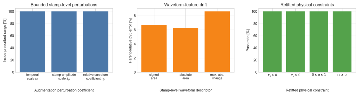
In the validation, these non-physical cases did not occur. All augmented stamps satisfy the constraints τ 1 > 0 , τ 2 > 0 , 0 α 1 and τ 2 τ 1 . The signs of the fitted polarization endpoints, P and P T , also remain identical to the corresponding parent-stamp signs in all augmented cases. The main stamp-level waveform descriptors stay close to the parent stamps: the parent-relative 95th-percentile errors are 6.27 % for the absolute stamp-area feature, 6.70 % for the signed stamp-area feature, and 8.60 % for the maximum absolute stamp change. In robust nearest-neighbor feature space, 83.9 % of the augmented stamps remain closest to their own parent stamp and 87.5 % remain closest to an original stamp from the same measurement file.
Figure 8 summarizes this validation by showing the perturbation bounds, the parent-relative waveform-feature drift, and the physical constraint pass ratios. These checks support the interpretation that augmentation acts as local regularization around measured recovery stamps, not as an expansion of the underlying electrochemical state space, cell population, or independently observed degradation states. They also support assigning the original class label to the augmented stamps. Accordingly, the increase from 48 original retained recovery events to 490 total stamp instances is treated only as training-side regularization.
Thus, the augmented stamps remain physically meaningful because the augmentation is local, bounded, smooth, parent-stamp-based, and every augmented stamp passed the post hoc physical parameter checks.

4.2. Deep Sequence Classifiers and Evaluation Procedure

Three temporal model families are included in the comparison, gated recurrent units (GRUs), temporal convolutional networks (TCNs), and a TimesNet-based architecture [16,56,57,58]. Within the compact-variable setting, exploratory comparisons are carried out between the GRU, TCN, and TimesNet models. Within the combined input setting, a matched comparison has then been carried out between a combined input TimesNet, a combined input GRU, and a combined input multilayer perceptron (MLP). The combined input GRU has represented a recurrent alternative with gated sequence compression, whereas the combined input multilayer perceptron has represented a non-temporal dense baseline operating on flattened compact variables and waveform inputs. This second comparison has been necessary in order to establish whether the gain observed in the combined representation has originated from the representation itself, from temporal modeling, or from both.
The gated recurrent unit represents the recurrent neural network family. For an input vector q k and a previous hidden state h k 1 , the GRU update is expressed by Equations (34)–(37):
r k = σ W r q k + U r h k 1 + b r ,
u k = σ W u q k + U u h k 1 + b u ,
h ˜ k = tanh W h q k + U h ( r k h k 1 ) + b h ,
h k = ( 1 u k ) h k 1 + u k h ˜ k ,
in which r k represents the reset gate, u k denotes the update gate, ⊙ denotes element-wise multiplication, and σ ( · ) represents the logistic sigmoid function [56,57]. The last hidden state, or a pooled hidden representation, is passed to the classification head. The GRU is included because gated recurrence can capture ordered dependencies among adjacent polarization stamps with a small number of trainable parameters.
The temporal convolutional network represents the convolutional sequence-modeling family. A dilated temporal convolution at layer is given by Equation (38),
h k ( ) = φ i = 0 K 1 W i ( ) h k d i ( 1 ) + b ( ) ,
in which K denotes the kernel length, d denotes the dilation factor, φ ( · ) represents the nonlinear activation, and h k ( 0 ) = q k . Residual connections are used between temporal convolution blocks. Bai et al. have shown that temporal convolutional networks can provide strong sequence-modeling performance and longer effective memory than canonical recurrent networks in several sequence tasks [58]. In the present application, the TCN tests whether local patterns across neighboring polarization-state variables are sufficient for fault-related state-deviation detection.
The TimesNet-based classifier represents the period-aware time-series modeling family. TimesNet has been introduced to model temporal variation by transforming a one-dimensional time series into multiple two-dimensional tensors according to dominant periods [16]. Recent studies have also applied TimesNet-type temporal modeling to lithium-ion battery applications, including state-of-health estimation, which supports its use as a relevant deep time-series baseline in battery diagnostics [59]. In the present application, this mechanism is used primarily on the L = 128 -point waveform branch of each retained recovery event, where the local recovery curve contains the immediate post-switch transition, the short-time curvature, and the slower relaxation tail within a common event-level time axis. The event-order dimension n = 3 remains short and is not interpreted as the principal source of the spectral structure. For the waveform branch, let Q R L × d w denote the local event-level input matrix, where L = 128 is the waveform-axis length and d w indexes the retained event channels entering the TimesNet block. The amplitude spectrum is obtained by applying the fast Fourier transform (FFT) to the discrete event-level waveform, as given by Equation (39) below,
A = Avg FFT ( Q ) ,
in which averaging is performed over the variable dimension. The K p dominant frequencies are selected from A , and the corresponding periods are computed by Equation (40) as follows:
p j = L f j , j = 1 , , K p .
For each selected period, the input sequence is padded when necessary and reshaped into a two-dimensional tensor (see Equation (41)).
Q 2 D ( j ) = Reshape p j Pad ( Q )
A two-dimensional convolutional block then extracts intra-period and inter-period variation (Equation (42)):
Y 2 D ( j ) = Conv2D j Q 2 D ( j ) .
After inverse reshaping, the outputs are combined by amplitude-based weights by Equation (43):
Y = j = 1 K p ω j Restore Y 2 D ( j ) , ω j = exp ( A f j ) r = 1 K p exp ( A f r ) .
This mechanism is suitable for the present task because the retained recovery waveform may contain repeated local patterns across multiple characteristic timescales within the 128-point event-level time axis, while the compact variables provide a lower-dimensional summary of the same recovery event. In the combined input setting, the same period-aware mixing therefore tests whether the immediate transition, short-time curvature, and slower relaxation tail of the waveform branch add discriminative information beyond the compact fitted variables. The TimesNet model therefore provides a structured temporal-mixing model for the event-level recovery waveform and the ordered recovery-stamp sequence.
The evaluation logic remains intentionally strict on the test side. Training and validation subsets contain original and augmented sequences, whereas the final test subset contains only original, non-augmented sequences from held-out base sequence groups. To evaluate the models on genuinely unseen original sequence groups, the final test subset has been constructed separately from the main training and validation pool. In the present corpus, one original base group gives rise to several closely related original sequences, and each of those may also generate multiple augmented variants. If such related samples appear on both sides of the evaluation, the reported test accuracy can become overly optimistic because the test data remain too similar to the training data [60]. To avoid this leakage, all variants derived from a selected base group have been kept on one side only. The test side has then been formed from one unseen reference group and a small number of unseen non-reference groups, while the remaining groups have been left available for training and validation. Under this construction, the strict held-out original-only test subset contains six sequences, comprising one reference and five non-reference sequences. The principal scalar metric is therefore balanced accuracy (BA), given by Equation (44),
BA = 1 2 TP TP + FN + TN TN + FP ,
because the class proportions have not been equal. Here, TP , FN , TN , and FP denote true positives, false negatives, true negatives, and false positives, respectively. The macro-averaged F1 score is computed by Equation (45) below:
F 1 macro = 1 2 c = 0 1 2 Precision c Recall c Precision c + Recall c .
The small strict test size is therefore a consequence of the leakage-control rule rather than a random reduction of the available data. The strict held-out subset provides an original sequence check of separability, while augmented variants are used only as training-side local regularization around measured recovery stamps and are not counted as independent electrochemical evidence. Accordingly, the deep learning results are interpreted comparatively, through repeated-seed behavior, optimization stability, and posterior separation, not as deployment-level generalization.

5. Results

5.1. Event Corpus, Augmentation, and Derived Sequence Set

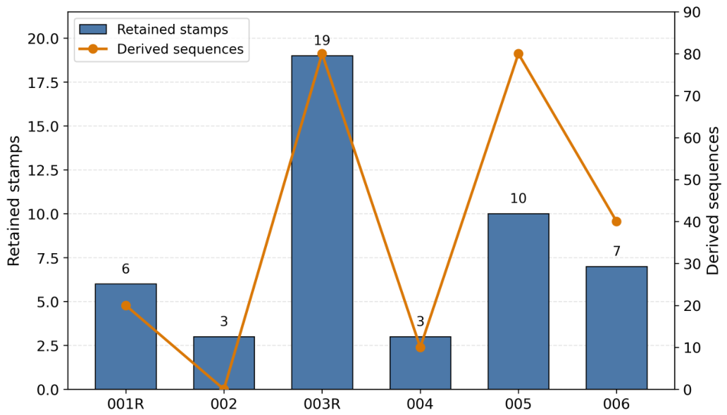
The final curated corpus contains 48 valid retained recovery stamps extracted from six documented cells. According to the retained-stamp technical labels, the event composition has been 39.6 % low-voltage manual step (LVM-step), 29.2 % multisine, 12.5 % manual step, 10.4 % bulk step, and 8.3 % composite step. At protocol-family level, these records correspond to four measurement classes: Manual PT, Stress PT (sq.), Stress msine, and Stress PT-msine. Augmentation has increased the stamp count to 490. The resulting sequence set contains 230 sequences, of which 23 have been original and 207 augmented; 190 sequences have contained three ordered events and 40 have contained five ordered events. Figure 9 shows that both event-level and sequence-level support have been unevenly distributed across cells. The largest event-level support has come from the LiFePO4 reference-consistent cell, Cell 003, while the non-reference cells have remained unevenly represented. Cell 006 did not contribute an original sequence under the adopted within-record sequence-construction rule, even though valid retained events were available at the event level. This asymmetry has limited the effective support of several cells and has therefore remained relevant in every subsequent interpretation.

5.2. Quality of the Recovery-Model Fit and Augmentation Assessment

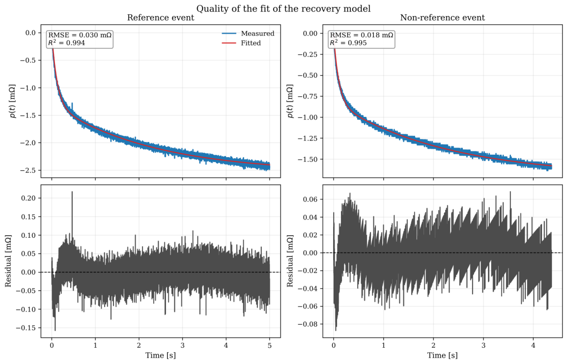
The adequacy of the two-timescale recovery model is first examined on original retained events. Figure 10 compares the measured current-normalized recovery curve p ( t ) with the fitted curve p ^ ( t ) for one reference event and one non-reference event, while the lower panels show the corresponding residuals. In both examples, the fitted curve follows the measured recovery closely over the 5 s fitting interval, and the residual remains small relative to the recovery amplitude. This supports the use of the fitted compact variables in the subsequent classification stage, because the model reproduces the dominant short-time and slower recovery behavior with acceptable fidelity on original, non-augmented events.
This subsection also assesses the practical role of augmentation by using a compact-feature comparison. Random forest, k-nearest neighbors, support vector machine (SVM) with radial-basis-function (RBF) kernel (SVM-RBF), logistic regression, and a most-frequent baseline are used as compact-feature sensitivity probes to test whether augmentation changes the decision boundary in a model-dependent or model-independent manner. The same leave-one-record-out protocol is used in both settings. Test folds contain only original, non-augmented sequences; augmentation is applied only to the training folds. Table 3 reports aggregated balanced accuracy over the original held-out sequence predictions.

5.3. Event-Level State Shift and Compact-Variable Behavior

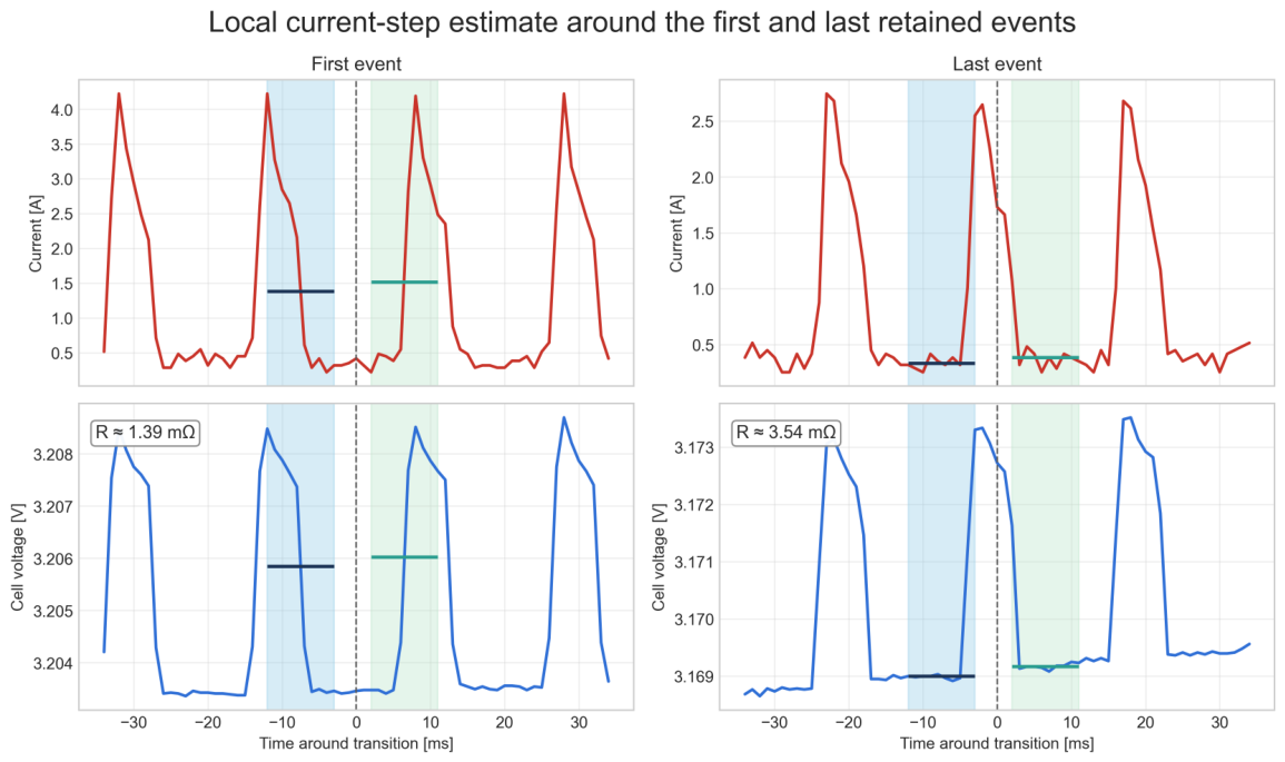
The event-level representation has remained physically interpretable at both the immediate transition scale and the subsequent recovery scale. Figure 11 compares the first and last retained transition events of a representative LiFePO4 bulk-step record from Cell 003. The apparent immediate-resistance estimate has been defined by Equation (46),
R inst = Δ V 0 Δ I 0 ,
in which Δ V 0 and Δ I 0 denote median pre-transition and post-transition voltage and current differences computed in short windows around the switching instant. The estimate has increased from approximately 1.39 m Ω at the beginning of the record to approximately 3.54 m Ω at the end. The later transition therefore indicates a larger local voltage-step-to-current-step ratio within the same dynamic record. This ratio is used only as a contextual state-shift indicator, because pulse-based resistance depends on SOC, temperature, the selected timescale, and the measurement procedure.
At the compact-variable level, the combination in Equation (47) has remained the most useful low-dimensional representation.
z = τ 1 α A p T
The compact variables retain one fast dynamical quantity, one recovery-shape quantity, and one signed-area quantity. Earlier exploratory analyses have shown that this triplet remains more stable than alternative three-dimensional combinations involving P T , particularly under limited sample support. The compact variables have therefore been retained as the structured branch of the final combined representation.

5.4. Current-Normalized Recovery-Amplitude Baseline

Figure 12 examines whether a single scalar recovery-amplitude quantity can account for the observed class separation. For this purpose, a current-normalized recovery-amplitude index is defined for each retained event given by Equation (48),
R a , k = Δ V k Δ I k ,
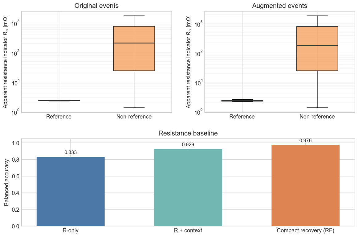
in which Δ V k denotes the retained recovery-amplitude change of event k and Δ I k represents the associated current step. This quantity is not interpreted as a DC internal resistance and not as an alternating-current (AC) impedance; it is used here only as a current-normalized recovery-amplitude index. The upper panel of Figure 12 shows that the non-reference events occupy a substantially broader and higher-valued index range than the reference events in both the original and the augmented event sets. The lower panel of Figure 12 confirms this quantitatively under the same leave-one-record-out protocol used for the sequence baselines: a conservative logistic index-only model based on the sequence mean of R a , k reached a balanced accuracy of 0.833 , while the corresponding index-plus-context model, obtained by adding mean current amplitude, mean relaxation length, and measurement type, reached 0.929 . The compact recovery representation nevertheless remained slightly stronger in the previously reported random forest comparison ( BA = 0.976 ). The present result therefore suggests that the current-normalized recovery amplitude is informative, but does not fully replace the recovery representation.

5.5. Deep Representation Comparison

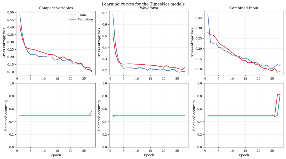
The principal deep learning result has been obtained from an input representation comparison using the same TimesNet-based encoder configuration. Figure 13 shows the learning curves of the TimesNet model for compact variables only, waveform only, and the combined input. The compact variables have reduced the training loss, but the validation balanced accuracy has remained unstable and split-dependent. The waveform branch has converged to a low-variance regime, yet has remained close to chance level throughout training. The combined input has been the only setting in which validation loss has decreased while validation balanced accuracy has remained persistently above the chance regime. The waveform branch has therefore not been sufficiently informative in isolation, whereas the compact variables have remained informative but fragile. The strongest deep result has been obtained only when the compact variables and the local waveform have been used together.
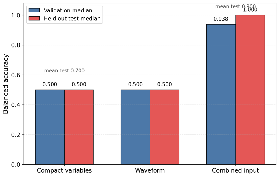
The same conclusion has been obtained from the repeated-seed summary displayed in Figure 14. This figure is used to expose seed-to-seed variability rather than to rely on a single favorable training run or on a single median point estimate. The waveform branch has remained at chance level, with median validation and held-out test balanced accuracy of 0.500 . The compact variables have been informative but unstable: the median validation and held-out test balanced accuracies have both remained 0.500 , although the mean held-out test balanced accuracy across repeated seeds has reached 0.700 because favorable splits have occurred for a subset of seeds. By contrast, the combined input has achieved median validation balanced accuracy of 0.938 and median held-out test balanced accuracy of 1.000 ; the corresponding mean held-out test balanced accuracy has been 0.900 . The reported median values should therefore be read together with the seed-to-seed spread shown in Figure 14, rather than as isolated point estimates. Overall, the repeated-seed behavior indicates that the two views carry complementary information: the compact-variable branch retains the dominant physics-informed recovery quantities, whereas the waveform branch preserves local transition morphology and short-time relaxation shape that the fitted compact variables alone have not fully retained.

5.6. Comparison with Other Deep Models

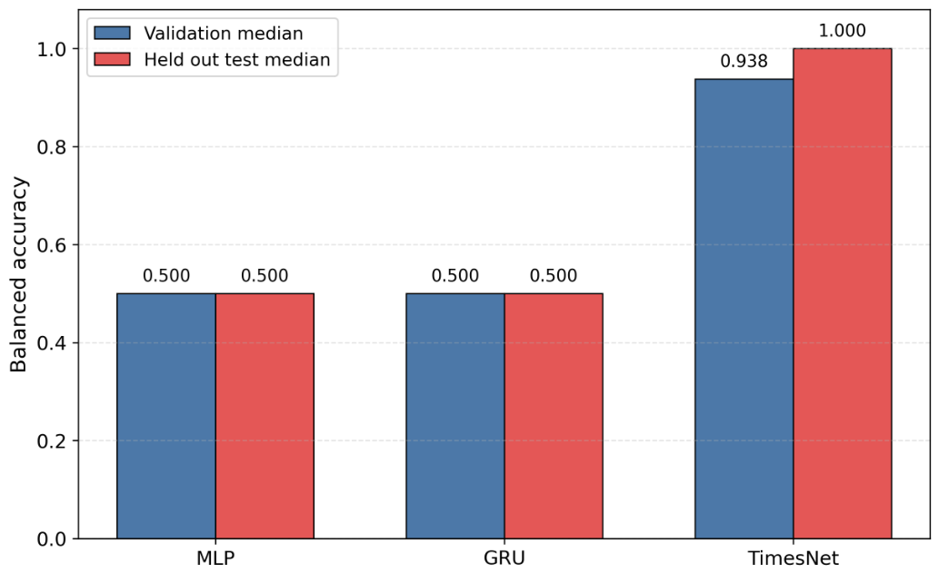
The relevance of the temporal encoder has then been assessed against alternative deep models in the combined input setting. Figure 15 shows the comparison between the multilayer perceptron, GRU, and TimesNet variants under the same repeated-seed protocol. In this setting, both the multilayer perceptron and the GRU have remained at chance level, whereas the TimesNet model has retained high validation and test balanced accuracy. The gain observed in the combined setting has therefore not arisen solely from adding a waveform branch. Rather, the combined representation has required a temporal encoder capable of exploiting heterogeneous local structure in the post-transition waveform, and that role has been fulfilled only by TimesNet in the present data regime.
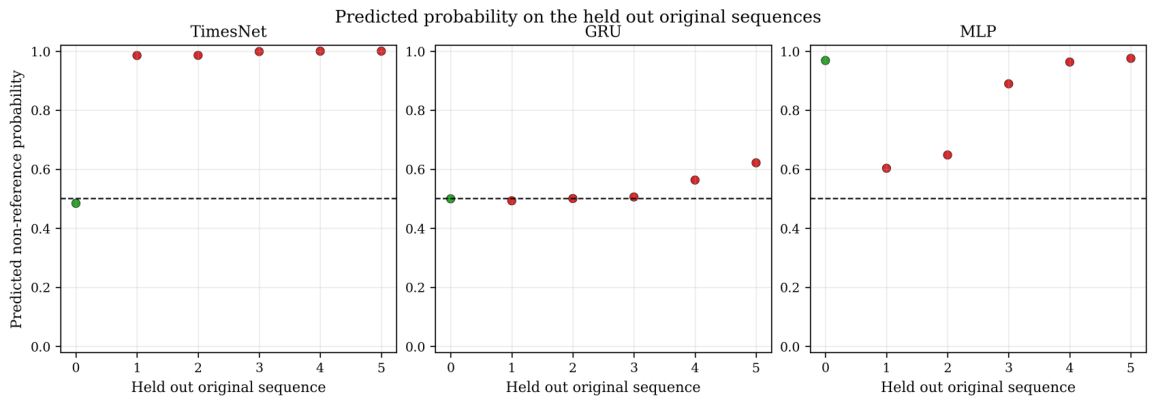
The combined input comparison is reflected directly in Figure 15. Across repeated seeds, the combined input GRU and combined input multilayer perceptron have both produced median validation and test balanced accuracy of 0.500 , whereas the combined input TimesNet has reached median validation balanced accuracy of 0.938 and median held-out test balanced accuracy of 1.000 . The posterior separation on the strict held-out original-only subset, shown in Figure 16, has reinforced the same interpretation. The TimesNet model has produced the clearest separation between the one held-out reference sequence and the five held-out non-reference sequences in the representative run. The GRU has kept all six posterior values in a narrow band around the decision threshold, whereas the multilayer perceptron has driven both classes towards high non-reference posterior values. The advantage of TimesNet has therefore not been restricted to one scalar score; it has also appeared in the posterior geometry of the held-out original-only subset.
Table 4 summarizes the position of the present result relative to related state-of-the-art directions.
For context, the classical compact-variable baselines evaluated under the stricter record-held-out assessment have remained strong on the 23-sequence original-only test set, with balanced-accuracy values of 0.976 for random forest, 0.905 for k-nearest neighbors, and 0.833 for the radial-basis SVM. Those results have indicated that the compact physics-informed representation has already contained substantial discriminative information. The deep learning results have therefore been interpreted differently. The combined compact-variable and waveform representation is used most effectively by the period-aware TimesNet encoder, whereas the simpler GRU and multilayer perceptron alternatives remain at chance-level performance in the combined input setting.
At implementation level, high-rate acquisition belongs to the event-capture layer, whereas the learning input remains compact. The proposed representation stores fitted recovery variables and a resampled local waveform rather than continuous 10 kHz records. This separation reduces storage and communication requirements and supports event-triggered battery diagnostics.
Taken together, the results have supported four observations. First, the retained recovery events have contained measurable and physically interpretable information at both the immediate-resistance and recovery-shape levels. Second, the compact variables have remained useful but insufficiently stable when used in isolation. Third, the waveform branch has not been discriminative enough in isolation. Fourth, the combined compact-variable and waveform representation has yielded the strongest and most stable deep learning result, and that benefit has been realized only when the combined representation has been paired with a TimesNet encoder rather than with simpler GRU or multilayer perceptron alternatives. The present findings have therefore supported the use of a combined physics-informed and waveform-aware representation for AI-based cell-level deviation detection. The uncertainty associated with the small original-only test subset is quantified next.
The strict held-out original-only test subset contains only six sequences, consisting of one reference and five non-reference sequences. This makes the scalar test score highly discrete: one non-reference error changes balanced accuracy by 0.1 , whereas one reference error changes balanced accuracy by 0.5 . Table 5 reports Wilson 95 % confidence intervals for the class-wise recalls of the representative strict test confusion matrix in which all six original sequences are correctly classified. These intervals use only original held-out sequences; augmented samples are not treated as independent observations for uncertainty estimation.

5.7. TimesNet Input-Sensitivity Analysis

To provide a more explicit interpretation of the combined input TimesNet decision rule, this subsection introduces a perturbation-based input-sensitivity analysis. The analysis is carried out on the repeated-seed validation splits used during model selection, not on the six-sequence strict held-out test subset alone. This choice avoids drawing component-level interpretation from the very small strict test set. At the same time, the analysis is not interpreted as an independent grouped-generalization proof, because the repeated-seed validation split is not a fully group-held-out split and may share original base groups with the training subset. The analysis is therefore used only as a validation-side sensitivity probe of the trained decision rule.
For each repeated-seed TimesNet model, the best validation checkpoint is retained and re-evaluated after targeted input perturbations. The unperturbed and perturbed scores are computed on the same validation subset and with the same trained checkpoint, so the reported drops are paired within each seed. In the compact-variable branch, τ 1 , α , and A p are replaced one at a time by their corresponding training-subset mean values. These replacement values are computed only from the training subset of the corresponding seed split. In the waveform branch, the resampled 5 s recovery waveform is divided into three physically interpretable regions: immediate transition and early recovery ( 0.0 0.5 s ), short-time curvature ( 0.5 2.0 s ), and slower relaxation tail ( 2.0 5.0 s ). Each waveform region is replaced by the training-subset mean waveform profile at the same relative time indices.
The balanced-accuracy drop is computed as
Δ BA = BA unperturbed BA perturbed ,
and the macro- F 1 drop is computed analogously. Larger drops therefore indicate stronger validation-side sensitivity to the perturbed compact variable or waveform region. Small or zero drops indicate that the component is weakly used, redundant with the remaining inputs, or difficult to assess robustly under the small validation support.
Figure 17 shows that the waveform-only TimesNet is insensitive to regional waveform masking. This result is consistent with the weak standalone performance of the waveform-only setting and should not be interpreted as evidence that the recovery waveform is physically irrelevant. Rather, it indicates that, under the present small-data validation setting, the waveform-only branch does not learn a stable discriminative rule.
The combined input TimesNet shows a different sensitivity pattern. Replacing either τ 1 or A p causes the largest compact-branch drops, with a mean validation balanced-accuracy drop of 0.277 and a median drop of 0.450 across repeated seeds. Replacing α produces no measurable drop under the same analysis. This suggests that, in the present validation setting, the combined model relies more strongly on the fast recovery timescale and signed recovery-area information than on the mixing-weight parameter alone. The result is interpreted cautiously because the seed-to-seed variability remains high.
In the waveform branch of the combined input TimesNet, masking the immediate transition and early recovery region ( 0.0 0.5 s ) produces no measurable drop. In contrast, masking the short-time curvature region ( 0.5 2.0 s ) or the slower relaxation tail ( 2.0 5.0 s ) produces a mean validation balanced-accuracy drop of 0.185 . The median drop remains zero for these waveform-region perturbations, which confirms that the estimate is noisy and seed-dependent. Nevertheless, the non-zero mean drops suggest that the combined TimesNet can exploit later recovery-shape information when this waveform information is supplied together with the fitted compact variables.
Overall, this analysis supports the interpretation that the combined input TimesNet does not rely on the immediate voltage transition alone. Instead, its validation-side decision rule is most sensitive to the fitted recovery variables τ 1 and A p , with additional but less stable sensitivity to the short-time curvature and slower-tail waveform regions.

6. Discussion

The present results indicate that short post-load recovery events can provide diagnostically useful inputs for AI-based lithium-ion cell screening. In the proposed method, the post-load recovery segment forms an intermediate representation between raw voltage traces and scalar resistance indicators. The immediate transition provides a resistance-related view of the cell state, whereas the subsequent recovery segment preserves information on fast and slower polarization dynamics.
The current-normalized recovery-amplitude analysis shows that a single scalar recovery index already provides a meaningful reference-separation baseline in the present corpus. The conservative logistic model based only on the sequence mean of R a , k reached a balanced accuracy of 0.833 , and the corresponding index-plus-context model reached 0.929 . These values show that the reference and non-reference classes are not separated by an artificial neural network effect alone. In contrast to a purely scalar screening rule, however, the compact recovery representation retains additional temporal information through τ 1 , α , and A p . The previously reported random forest comparison on the compact recovery variables reached 0.976 balanced accuracy, which suggests that the recovery-shape and signed recovery area contain information that is not fully reduced to a single current-normalized amplitude value. The proposed representation should therefore be viewed as a richer and more physically expressive extension of scalar screening. Its main advantage is that it transforms a short transient measurement into a small set of physically interpretable variables, thereby reducing the dependence on large labeled fault datasets while still retaining information that is relevant for AI-based discrimination.
The deep representation comparison shows that the input representation is more important than the size of the neural model in the present data regime. The waveform-only TimesNet branch remained at chance level, with median validation and held-out balanced accuracy of 0.500 . The compact fitted-variable branch was informative but unstable, with median validation and held-out balanced-accuracy values of 0.500 and a mean held-out balanced accuracy of 0.700 . By comparison, the combined fitted-variable and waveform representation reached a median validation balanced accuracy of 0.938 , a median held-out test balanced accuracy of 1.000 , and a mean held-out test balanced accuracy of 0.900 . This difference supports the interpretation that the fitted recovery variables and the local waveform morphology contain complementary information. The fitted variables preserve the physically interpretable polarization response and signed recovery area, whereas the waveform branch preserves transition morphology, short-time curvature, and relaxation-shape information that may be partly lost during low-dimensional fitting.
The comparison between the temporal models further supports this interpretation. In the combined input setting, the combined input GRU and combined input multilayer perceptron both remained at 0.500 median balanced accuracy, whereas the combined input TimesNet retained high validation and test performance. This result suggests that the observed gain did not arise simply from adding more input variables. Rather, discrimination improved when the combined representation was paired with a temporal encoder capable of mixing heterogeneous local structures in the recovery waveform. TimesNet is therefore used here as a structured temporal-mixing model for short recovery events, not as a claim of electrochemical periodicity.
From the state-of-the-art comparison, the position of the present work can be defined more precisely. Previous dynamic-load and multisine studies have mainly addressed terminal-voltage prediction, SOC prediction, or equivalent-circuit parameterization under realistic vehicle-like operating conditions [8,9,20,27]. Recent polarization-aware studies have addressed polarization-voltage characterization or SOH estimation, often under charging or model-identification conditions [44,47]. Recent AI-based fault-diagnosis studies have demonstrated the strength of temporal and model-constrained deep learning at a much larger EV-data scale [5,6,7]. The present study occupies a narrower but distinct position. It uses short recovery events after dynamic pulse–multisine loading and evaluates reference-centered degradation-related cell-level discrimination. Its strength is not dataset scale, but the combination of physically interpretable recovery variables with waveform morphology for AI-oriented cell screening. The two-timescale recovery model further clarifies this positioning. Exponential relaxation models and multi-resistor–capacitor (RC) equivalent-circuit representations are well established in battery modeling, whereas their use here is directed towards diagnostic representation learning. Here, the fitted quantities are used as compact recovery-state variables extracted from short, high-resolution post-load events. Combined with the local waveform, they provide an AI-oriented representation that preserves the physical meaning of polarization recovery while limiting the dimensionality of the learning problem. The application value follows from this intermediate position. In industrial-electronics and BMS-oriented use, the method could serve as a rapid screening layer between simple scalar checks and more expensive diagnostic procedures such as full EIS or detailed laboratory characterization. A practical implementation could use short and controlled load interruptions, or select naturally occurring EV transient events to extract recovery segments and estimate whether a cell remains reference-consistent within its family. The 10 kHz acquisition rate is used here as a laboratory-resolution setting to resolve the current-interruption instant, the immediate voltage transition, the short-time curvature, and the slower recovery tail within the same event. This does not imply continuous high-rate storage in a BMS implementation, because the diagnostic object is a short recovery event and the final representation is reduced to compact fitted variables and a resampled local waveform. A practical implementation can therefore be based on event-triggered short-window acquisition around selected load-transition or recovery events. Recent onboard diagnostic studies have shown that module-level battery measurements can be adapted to embedded sampling and hardware-bandwidth constraints, for example by using equivalent sampling and commercially available battery-monitoring electronics [34]. Such a procedure would be most relevant for end-of-line inspection, service diagnostics, second-life sorting, and early warning in systems where full impedance testing is not available during operation. The method is also suitable for integration with existing diagnostic measurement software because it uses voltage and current signals that are already available in many battery test systems.
Methodologically, the proposed representation reduces the learning problem before classification. The measurement procedure exposes the recovery dynamics, the two-timescale model converts them into compact variables with physical meaning, and the deep model operates on this reduced representation together with the local waveform. This structure is consistent with practical fault screening, where labeled fault data are limited and early deviations must remain interpretable.
Several limitations remain. The retained corpus contained only 48 valid original recovery stamps from six documented cells, and the derived sequence set contained only 23 original sequences before augmentation. The strict held-out original-only test subset contained six sequences, with one reference and five non-reference cases. For this reason, the reported deep learning scores should be interpreted as comparative pilot evidence rather than broad generalization evidence. In addition, the class label represents reference-centered degradation-related deviation and not mechanism-specific fault identification. A manifest-level split-feasibility audit was conducted to avoid overstating generalization beyond the available corpus. The audit considered base-sequence-group, record-held-out, cell-held-out, family-held-out, and chemistry-held-out splits. For each candidate held-out group, the test side contained only original sequences, while augmented variants derived from held-out original base sequences were excluded from training. Table 6 shows that several candidate split levels do not provide folds with both classes on the test side, and the family- and chemistry-level splits are confounded with the limited reference-cell support. Balanced accuracy is therefore not meaningful as a fold-level performance metric for those split levels. Accordingly, cell-, family-, and chemistry-level generalization is treated as a required future validation step rather than as a demonstrated result of the present pilot study. Because all measurements were acquired under approximately constant laboratory temperature conditions, the present study does not evaluate temperature-dependent variation of the recovery features, which is expected to influence the relaxation dynamics and would require dedicated multi-temperature validation.
Future work should therefore extend the cell population, include strict cell-held-out and chemistry-held-out tests, and connect the class labels to independent capacity, DCIR, EIS, temperature, cycling history, or post-mortem evidence. Further development should also include uncertainty calibration, SOC- and temperature-dependent normalization, explicit comparison with HPPC and EIS references, and embedded implementation tests under realistic BMS constraints.

7. Conclusions

This paper has investigated lithium-ion cell degradation-related deviation through high-resolution polarization recovery events measured after pulse, stress, and pulse–multisine loading. Previously developed dynamic excitation and diagnostic measurement capabilities have been used here for AI-based reference-centered detection of degradation-related cell behavior from post-load recovery segments [20,27,28].
The main contribution is a recovery-stamp representation for battery fault screening. Each retained load removal event is converted into a signed current-normalized polarization stamp p ( t ) , described by a constrained two-timescale recovery model, and represented by compact variables together with the local recovery waveform. In contrast to scalar pulse-resistance evaluation or direct recovery-curve fitting alone, the proposed diagnostic object retains three coupled levels of information: the signed current-normalized stamp, the fitted compact recovery state, and the resampled local waveform used in ordered sequence-level classification.
The 10 kHz burst acquisition preserves the effective transient signature, and the subsequent fitting and resampling reduce this signature to compact event tokens for sequence-level AI analysis.
The results have shown that the recovery stamps contain measurable state information beyond a single scalar amplitude measure. In the representative Cell 003 LiFePO4 bulk-step record, the apparent immediate-resistance estimate changed from approximately 1.39 m Ω to approximately 3.54 m Ω , indicating a change in the local voltage-step-to-current-step ratio rather than a direct change in intrinsic cell resistance. The current-normalized recovery-amplitude index has already been informative, reaching balanced accuracies of 0.833 without and 0.929 with operating context. In a separate classical reference comparison, the compact recovery representation has provided a strong baseline, with a random forest balanced accuracy of 0.976 . This result indicates that the fitted polarization stamp variables already contain substantial discriminative information.
The final deep learning comparison has focused on the compact-variable, waveform-only, and combined input settings, with TimesNet compared against GRU and multilayer perceptron alternatives in the combined input case. The waveform-only and simpler combined input models have remained at chance level, whereas the combined fitted-variable and waveform TimesNet model has reached a median validation balanced accuracy of 0.938 and has shown stable performance across repeated runs. This shows that the joint stamp-and-waveform representation is exploited most effectively by the TimesNet temporal-mixing model, whereas the GRU and multilayer perceptron alternatives remain less effective in the combined input setting. TimesNet has therefore been useful as a structured temporal-mixing model for recovery-stamp sequences. The validation-side input-sensitivity audit suggests that the combined model is most sensitive to the fitted recovery variables τ 1 and A p , with additional but less stable sensitivity to the short-time curvature and slower relaxation-tail waveform regions.
The present evidence supports degradation-related state-deviation screening, rather than direct identification of solid–electrolyte interphase (SEI) growth, lithium plating, contact loss, active-material loss, or other specific electrochemical fault mechanisms. The dataset remains limited in size, with 48 valid original recovery stamps and 23 original sequences before augmentation. Therefore, the reported deep learning scores should be interpreted as comparative pilot evidence rather than proof of broad chemistry-independent generalization.
The proposed representation is therefore most relevant for diagnostic settings where only short voltage-current windows are available and full impedance measurements are not practical. Such settings include service diagnostics, second-life sorting, end-of-line inspection, and event-triggered BMS-oriented screening.
Future work should expand the measurement set, include independent aging histories, and validate the decision rule against capacity, direct-current internal resistance (DCIR), EIS, temperature, cycling history, and post-mortem references. The next technical step is the evaluation of strict cell-held-out and family-held-out protocols under controlled SOC and temperature ranges. Overall, dynamically excited polarization recovery provides a compact intermediate representation between scalar resistance-based screening and full impedance-based diagnostics.

Funding

This research received no external funding.

Institutional Review Board Statement

Not applicable.

Data Availability Statement

The data presented in this study are available from the corresponding author upon reasonable request.

Conflicts of Interest

The author declares no conflicts of interest.

Abbreviations

The following abbreviations are used in this manuscript:
ACAlternating current
ADCAnalog-to-digital converter
AIArtificial intelligence
BABalanced accuracy
BMSBattery management system
CIConfidence interval
DCDirect current
DCIRDirect-current internal resistance
ECMEquivalent-circuit model
EISElectrochemical impedance spectroscopy
EVElectric vehicle
FFTFast Fourier transform
FNFalse negative
FPFalse positive
GRUGated recurrent unit
H20 20 Ah LiFePO4 cell family
HEVHybrid electric vehicle
HPPCHybrid Pulse Power Characterization
IECInternational Electrotechnical Commission
ISOInternational Organization for Standardization
K40Kokam 40 Ah cell family
LFPLithium iron phosphate
Li-ionLithium-ion
LVMLow-voltage manual
MLMachine learning
MLPMultilayer perceptron
msineMultisine
NMCNickel manganese cobalt oxide
OCVOpen-circuit voltage
PDIPolarization Deviation Index
PPCPulse Power Characterization
PTPulse train
RBFRadial basis function
RCResistor–capacitor
SEISolid-electrolyte interphase
SOCState of charge
SOHState of health
sq.Square-wave
SVMSupport vector machine
TCNTemporal convolutional network
TNTrue negative
TPTrue positive
vec.Test-vector-defined
VIVirtual instrument
WLTPWorldwide Harmonized Light Vehicles Test Procedure

References

  1. Samanta, A.; Chowdhuri, S.; Williamson, S.S. Machine Learning-Based Data-Driven Fault Detection/Diagnosis of Lithium-Ion Battery: A Critical Review. Electronics 2021, 10, 1309. [Google Scholar] [CrossRef] [Scilit]
  2. Yu, Q.; Wang, C.; Li, J.; Xiong, R.; Pecht, M. Challenges and Outlook for Lithium-Ion Battery Fault Diagnosis Methods from the Laboratory to Real World Applications. eTransportation 2023, 17, 100254. [Google Scholar] [CrossRef] [Scilit]
  3. Zou, B.; Zhang, L.; Xue, X.; Tan, R.; Jiang, P.; Ma, B.; Song, Z.; Hua, W. A Review on the Fault and Defect Diagnosis of Lithium-Ion Battery for Electric Vehicles. Energies 2023, 16, 5507. [Google Scholar] [CrossRef] [Scilit]
  4. Kaleem, M.B.; Zhou, Y.; Jiang, F.; Liu, Z.; Li, H. Fault Detection for Li-Ion Batteries of Electric Vehicles with Segmented Regression Method. Sci. Rep. 2024, 14, 31922. [Google Scholar] [CrossRef] [Scilit]
  5. Zhao, J.; Feng, X.; Wang, J.; Lian, Y.; Ouyang, M.; Burke, A.F. Battery Fault Diagnosis and Failure Prognosis for Electric Vehicles Using Spatio-Temporal Transformer Networks. Appl. Energy 2023, 352, 121949. [Google Scholar] [CrossRef] [Scilit]
  6. Zhang, J.; Wang, Y.; Jiang, B.; He, H.; Huang, S.; Wang, C.; Zhang, Y.; Han, X.; Guo, D.; He, G.; et al. Realistic Fault Detection of Li-Ion Battery via Dynamical Deep Learning. Nat. Commun. 2023, 14, 5940. [Google Scholar] [CrossRef] [Scilit]
  7. Cao, R.; Zhang, Z.; Shi, R.; Lu, J.; Zheng, Y.; Sun, Y.; Liu, X.; Yang, S. Model-Constrained Deep Learning for Online Fault Diagnosis in Li-Ion Batteries over Stochastic Conditions. Nat. Commun. 2025, 16, 1651. [Google Scholar] [CrossRef] [Scilit]
  8. Widanage, W.D.; Barai, A.; Chouchelamane, G.H.; Uddin, K.; McGordon, A.; Marco, J.; Jennings, P.A. Design and Use of Multisine Signals for Li-Ion Battery Equivalent Circuit Modelling. Part 1: Signal Design. J. Power Sources 2016, 324, 70–78. [Google Scholar] [CrossRef] [Scilit]
  9. Widanage, W.D.; Barai, A.; Chouchelamane, G.H.; Uddin, K.; McGordon, A.; Marco, J.; Jennings, P.A. Design and Use of Multisine Signals for Li-Ion Battery Equivalent Circuit Modelling. Part 2: Model Estimation. J. Power Sources 2016, 324, 61–69. [Google Scholar] [CrossRef] [Scilit]
  10. Qu, D.; Ji, W.; Qu, H. Probing Process Kinetics in Batteries with Electrochemical Impedance Spectroscopy. Commun. Mater. 2022, 3, 61. [Google Scholar] [CrossRef] [Scilit]
  11. Nováková, K.; Pražanová, A.; Stroe, D.I.; Knap, V. Review of Electrochemical Impedance Spectroscopy Methods for Lithium-Ion Battery Diagnostics and Their Limitations. Monatshefte Chem. Chem. Mon. 2024, 155, 227–232. [Google Scholar] [CrossRef] [Scilit]
  12. Faraji Niri, M.; Aslansefat, K.; Haghi, S.; Hashemian, M.; Daub, R.; Marco, J. A Review of the Applications of Explainable Machine Learning for Lithium-Ion Batteries: From Production to State and Performance Estimation. Energies 2023, 16, 6360. [Google Scholar] [CrossRef] [Scilit]
  13. Hao, Z.; Zhang, Q.; Wang, D.; Liu, S.; Yang, B.; Li, X. The Application of Pulse Response Analysis Method in Lithium-Ion Battery Modeling and State Estimation. J. Energy Storage 2024, 102, 114074. [Google Scholar] [CrossRef] [Scilit]
  14. Gasper, P.; Prakash, N.; Knutson, B.; Bethel, T.; Ramirez-Meyers, K.; Condon, A.; Attia, P.M.; Keyser, M. Searching for a Pulse: Evaluating the Use of Rapid DC Pulses for Diagnosing Battery Health, State-of-Charge, and Safety. J. Electrochem. Soc. 2025, 172, 060503. [Google Scholar] [CrossRef] [Scilit]
  15. Amri, A.; Hendri, Y.B.; Saputra, E.; Heltina, D.; Yin, C.Y.; Rahman, M.M.; Minakshi, M.; Mondinos, N.; Jiang, Z.T. Formation kinetics of sol-gel derived LiFePO4 olivine analyzed by reliable non-isothermal approach. Ceram. Int. 2022, 48, 17729–17737. [Google Scholar] [CrossRef] [Scilit]
  16. Wu, H.; Hu, T.; Liu, Y.; Zhou, H.; Wang, J.; Long, M. TimesNet: Temporal 2D-Variation Modeling for General Time Series Analysis. In Proceedings of the 11th International Conference on Learning Representations, Kigali, Rwanda, 1–5 May 2023. [Google Scholar] [CrossRef] [Scilit]
  17. Belt, J.R. Battery Test Manual for Plug-In Hybrid Electric Vehicles; Technical Report INL/EXT-07-12536 Rev. 2; Idaho National Laboratory: Idaho Falls, ID, USA, 2010. [Google Scholar]
  18. Krewer, U.; Röder, F.; Harinath, E.; Braatz, R.D.; Bedürftig, B.; Findeisen, R. Review—Dynamic Models of Li-Ion Batteries for Diagnosis and Operation: A Review and Perspective. J. Electrochem. Soc. 2018, 165, A3656–A3673. [Google Scholar] [CrossRef] [Scilit]
  19. Micari, S.; Foti, S.; Testa, A.; De Caro, S.; Sergi, F.; Andaloro, L.; Aloisio, D.; Leonardi, S.G.; Napoli, G. Effect of WLTP Class 3B Driving Cycle on Lithium-Ion Battery for Electric Vehicles. Energies 2022, 15, 6703. [Google Scholar] [CrossRef] [Scilit]
  20. Dineva, A.; Csomós, B.; Kocsis Sz., S.; Vajda, I. Investigation of the Performance of Direct Forecasting Strategy Using Machine Learning in State-of-Charge Prediction of Li-Ion Batteries Exposed to Dynamic Loads. J. Energy Storage 2021, 36, 102351. [Google Scholar] [CrossRef] [Scilit]
  21. ISO 12405-4:2018; Electrically Propelled Road Vehicles—Test Specification for Lithium-Ion Traction Battery Packs and Systems—Part 4: Performance Testing. International Organization for Standardization: Geneva, Switzerland, 2018.
  22. IEC 62660-1:2018; Secondary Lithium-Ion Cells for the Propulsion of Electric Road Vehicles—Part 1: Performance Testing. International Electrotechnical Commission: Geneva, Switzerland, 2018.
  23. IEC 62660-2:2018; Secondary Lithium-Ion Cells for the Propulsion of Electric Road Vehicles—Part 2: Reliability and Abuse Testing. International Electrotechnical Commission: Geneva, Switzerland, 2018.
  24. IEC 62660-3:2022; Secondary Lithium-Ion Cells for the Propulsion of Electric Road Vehicles—Part 3: Safety Requirements. International Electrotechnical Commission: Geneva, Switzerland, 2022.
  25. Schoukens, J.; Ljung, L. Nonlinear System Identification: A User-Oriented Road Map. IEEE Control Syst. Mag. 2019, 39, 28–99. [Google Scholar] [CrossRef] [Scilit]
  26. Firouz, Y.; Omar, N.; Goutam, S.; Timmermans, J.M.; Van den Bossche, P.; Van Mierlo, J. Measuring and Analysis of Nonlinear Characterization of Lithium-Ion Batteries Using Multisin Excitation Signal. World Electr. Veh. J. 2016, 8, 362–370. [Google Scholar] [CrossRef] [Scilit]
  27. Dineva, A. Advanced Machine Learning Approaches for State-of-Charge Prediction of Li-Ion Batteries under Multisine Excitation. In Proceedings of the 2021 17th Conference on Electrical Machines, Drives and Power Systems (ELMA), Sofia, Bulgaria, 1–4 July 2021; pp. 1–5. [Google Scholar] [CrossRef] [Scilit]
  28. Dineva, A.; Kocsis, Sz.S. Method for Diagnostic and Predictive Modelling of a Battery, in Particular an Electric Vehicle Lithium Battery, in a Dynamic Operating Environment, and Apparatus for Implementing the Method. Hungarian Patent HU231740B1, 10 November 2025. [Google Scholar]
  29. National Instruments. NI-9206 Specifications Updated 26 February 2026. Available online: https://www.ni.com/docs/en-US/bundle/ni-9206-specs/page/specs.html (accessed on 27 February 2026).
  30. National Instruments. NI-9206 Getting Started. Updated 9 October 2024. 2024. Available online: https://www.ni.com/docs/en-US/bundle/ni-9206-getting-started/page/overview.html (accessed on 21 February 2026).
  31. Howey, D.A.; Mitcheson, P.D.; Yufit, V.; Offer, G.J.; Brandon, N.P. Online Measurement of Battery Impedance Using Motor Controller Excitation. IEEE Trans. Veh. Technol. 2014, 63, 2557–2566. [Google Scholar] [CrossRef] [Scilit]
  32. Carkhuff, B.G.; Demirev, P.A.; Srinivasan, R. Impedance-Based Battery Management System for Safety Monitoring of Lithium-Ion Batteries. IEEE Trans. Ind. Electron. 2018, 65, 6497–6504. [Google Scholar] [CrossRef] [Scilit]
  33. Crescentini, M.; De Angelis, A.; Ramilli, R.; De Angelis, G.; Tartagni, M.; Moschitta, A.; Traverso, P.A.; Carbone, P. Online EIS and Diagnostics on Lithium-Ion Batteries by Means of Low-Power Integrated Sensing and Parametric Modeling. IEEE Trans. Instrum. Meas. 2021, 70, 2001711. [Google Scholar] [CrossRef] [Scilit]
  34. Zhang, S.; Wei, Z.; Zhang, L.; Hu, J.; Dai, R. Equivalent sampling-enabled module-level battery impedance measurement for in-situ lithium plating diagnostic. J. Power Sources 2024, 600, 234239. [Google Scholar] [CrossRef] [Scilit]
  35. Kokam Co., Ltd. SLPB 100216216H Cell Specification; Manufacturer Data Sheet; Public Mirror; Kokam Co., Ltd.: Suwon, Republic of Korea, n.d.; Available online: https://liionbms.com/pdf/kokam/SLPB100216216H.pdf (accessed on 15 April 2026).
  36. Khalid, A.; Kashif, S.A.R.; Ain, N.U.; Awais, M.; Smieee, M.A.; Carreño, J.E.M.; Vasquez, J.C.; Guerrero, J.M.; Khan, B. Comparison of Kalman Filters for State Estimation Based on Computational Complexity of Li-Ion Cells. Energies 2023, 16, 2710. [Google Scholar] [CrossRef] [Scilit]
  37. AA Portable Power Corp. Specification of High Power LFP Polymer Cell: 3.2 V 20 Ah (100122200-2C, 64 Wh, 40 A Rate) UN Approved; Public Product Specification for Model 100122200L; Prepared 2 January 2010; AA Portable Power Corp.: Richmond, CA, USA, 2010; Available online: https://www.batteryspace.com/prod-specs/5455.pdf (accessed on 16 March 2026).
  38. Routh, B.; Mitra, D.; Patra, A.; Mukhopadhyay, S. Extended Kalman Filter Based Estimation of the State of Charge of Lithium-Ion Cells Using a Switched Model. IFAC-Pap. 2020, 53, 13922–13927. [Google Scholar] [CrossRef] [Scilit]
  39. Dineva, A. Advances in Lithium-Ion Battery Management through Deep Learning Techniques: A Performance Analysis of State-of-Charge Prediction at Various Load Conditions. In Proceedings of the 2023 IEEE 17th International Symposium on Applied Computational Intelligence and Informatics (SACI), Timisoara, Romania, 23–26 May 2023; pp. 773–778. [Google Scholar] [CrossRef] [Scilit]
  40. Zhao, D.; Chen, W. Analysis of Polarization and Thermal Characteristics in Lithium-Ion Battery with Various Electrode Thicknesses. J. Energy Storage 2023, 71, 108159. [Google Scholar] [CrossRef] [Scilit]
  41. Zheng, J.; Lu, J.; Amine, K.; Pan, F. Depolarization Effect to Enhance the Performance of Lithium Ions Batteries. Nano Energy 2017, 33, 497–507. [Google Scholar] [CrossRef] [Scilit]
  42. Newman, J.; Tiedemann, W. Porous-Electrode Theory with Battery Applications. AIChE J. 1975, 21, 25–41. [Google Scholar] [CrossRef] [Scilit]
  43. Doyle, M.; Fuller, T.F.; Newman, J. Modeling of Galvanostatic Charge and Discharge of the Lithium/Polymer/Insertion Cell. J. Electrochem. Soc. 1993, 140, 1526–1533. [Google Scholar] [CrossRef] [Scilit]
  44. Xia, B.; Ye, B.; Cao, J. Polarization Voltage Characterization of Lithium-Ion Batteries Based on a Lumped Diffusion Model and Joint Parameter Estimation Algorithm. Energies 2022, 15, 1150. [Google Scholar] [CrossRef] [Scilit]
  45. Barai, A.; Widanage, W.D.; Marco, J.; McGordon, A.; Jennings, P.A. A Study of the Open Circuit Voltage Characterization Technique and Hysteresis Assessment of Lithium-Ion Cells. J. Power Sources 2015, 295, 99–107. [Google Scholar] [CrossRef] [Scilit]
  46. Voicila, T.I.; Enache, B.A.; Argyriou, V.; Sarigiannidis, P.; Pisla, M.A.; Seritan, G.C. Enhanced OCV Estimation in LiFePO4 Batteries: A Novel Statistical Approach Leveraging Real-Time Knee/Elbow Detection. Batteries 2025, 11, 186. [Google Scholar] [CrossRef] [Scilit]
  47. Wang, T.; Wu, Y.; Zhu, K.; Cen, J.; Wang, S.; Huang, Y. Deep Learning and Polarization Equilibrium Based State of Health Estimation for Lithium-Ion Battery Using Partial Charging Data. Energy 2025, 317, 134564. [Google Scholar] [CrossRef] [Scilit]
  48. Barai, A.; Uddin, K.; Widanage, W.D.; McGordon, A.; Jennings, P. A Study of the Influence of Measurement Timescale on Internal Resistance Characterisation Methodologies for Lithium-Ion Cells. Sci. Rep. 2018, 8, 21. [Google Scholar] [CrossRef] [Scilit] [PubMed]
  49. Seidenberg, J.R.; Mitsos, A.; Bongartz, D. Interpreting Concentration and Activation Overpotentials in Electrochemical Systems: A Critical Discussion. J. Electrochem. Soc. 2025, 172, 043506. [Google Scholar] [CrossRef] [Scilit]
  50. Bergveld, H.J.; Kruijt, W.S.; Notten, P.H.L. Battery Management Systems: Design by Modelling; Kluwer Academic Publishers: Dordrecht, The Netherlands, 2002. [Google Scholar] [CrossRef] [Scilit]
  51. Plett, G.L. Battery Management Systems, Volume I: Battery Modeling; Artech House: Norwood, MA, USA, 2015. [Google Scholar]
  52. Goldammer, E.; Kowal, J. Determination of the Distribution of Relaxation Times by Means of Pulse Evaluation for Offline and Online Diagnosis of Lithium-Ion Batteries. Batteries 2021, 7, 36. [Google Scholar] [CrossRef] [Scilit]
  53. Hu, X.; Zhang, K.; Liu, K.; Lin, X.; Dey, S.; Onori, S. Advanced Fault Diagnosis for Lithium-Ion Battery Systems: A Review of Fault Mechanisms, Fault Features, and Diagnosis Procedures. IEEE Ind. Electron. Mag. 2020, 14, 65–91. [Google Scholar] [CrossRef] [Scilit]
  54. Ngiam, J.; Khosla, A.; Kim, M.; Nam, J.; Lee, H.; Ng, A.Y. Multimodal Deep Learning. In Proceedings of the 28th International Conference on Machine Learning, Bellevue, WA, USA, 28 June–2 July 2011; pp. 689–696. [Google Scholar]
  55. Iwana, B.K.; Uchida, S. An Empirical Survey of Data Augmentation for Time Series Classification with Neural Networks. PLoS ONE 2021, 16, e0254841. [Google Scholar] [CrossRef] [Scilit]
  56. Cho, K.; van Merriënboer, B.; Gülçehre, Ç.; Bahdanau, D.; Bougares, F.; Schwenk, H.; Bengio, Y. Learning Phrase Representations Using RNN Encoder–Decoder for Statistical Machine Translation. In Proceedings of the 2014 Conference on Empirical Methods in Natural Language Processing; Association for Computational Linguistics: Stroudsburg, PA, USA, 2014; pp. 1724–1734. [Google Scholar] [CrossRef] [Scilit]
  57. Chung, J.; Gülçehre, Ç.; Cho, K.; Bengio, Y. Empirical Evaluation of Gated Recurrent Neural Networks on Sequence Modeling. arXiv 2014, arXiv:1412.3555. [Google Scholar] [CrossRef] [Scilit]
  58. Bai, S.; Kolter, J.Z.; Koltun, V. An Empirical Evaluation of Generic Convolutional and Recurrent Networks for Sequence Modeling. arXiv 2018, arXiv:1803.01271. [Google Scholar] [CrossRef] [Scilit]
  59. Wu, M.; Xia, J. State of Health Estimation Based on the TimesNet Model for Real-World Electric Vehicle Batteries. J. Renew. Sustain. Energy 2025, 17, 035701. [Google Scholar] [CrossRef] [Scilit]
  60. Joeres, R.; Blumenthal, D.B.; Kalinina, O.V. Data Splitting to Avoid Information Leakage with DataSAIL. Nat. Commun. 2025, 16, 3337. [Google Scholar] [CrossRef] [Scilit]
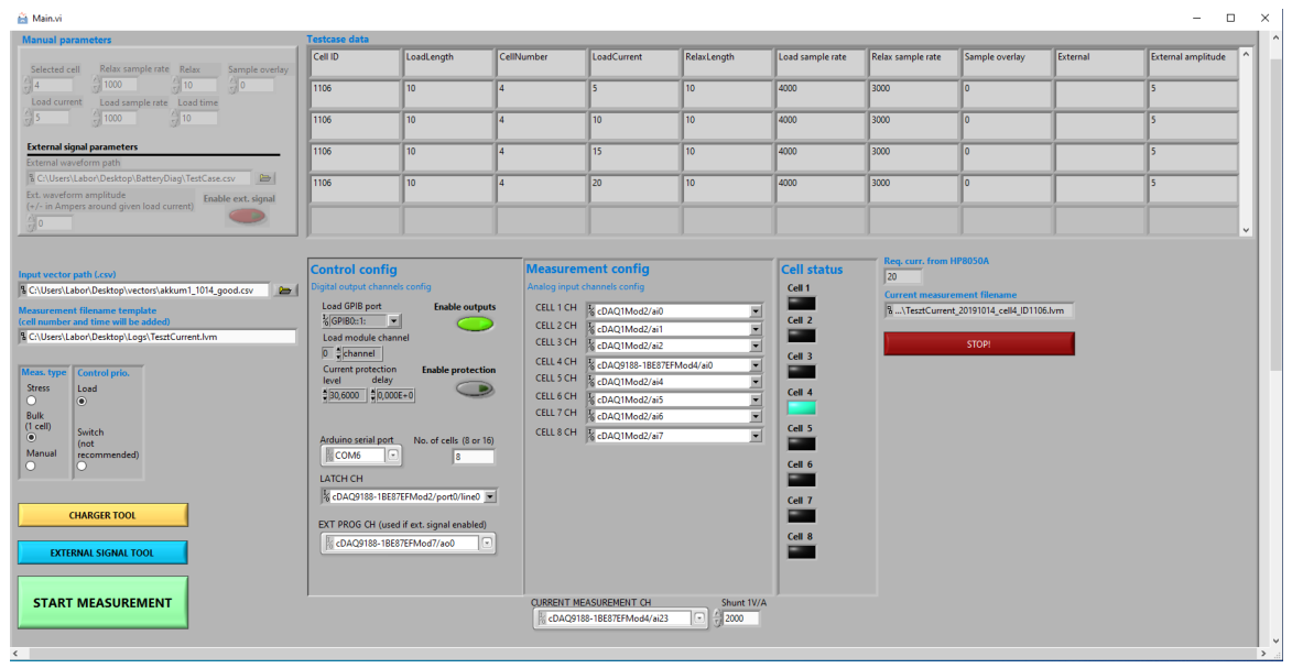
Figure 1. Main VI of the battery diagnostic measurement and control software [27,28]. The interface supports manual operation, automated test-vector execution, cell selection, sampling configuration, and monitoring of the measurement process.
Electronics 15 02291 g001
Figure 2. Signal generator VI used for configuring the externally programmed excitation waveform [28].
Electronics 15 02291 g002
Figure 8. Physical validation of the stamp-level augmentation procedure. The left panel verifies that the sampled s t , s p , and η p coefficients remain inside their prescribed ranges. The middle panel reports the parent-relative 95th-percentile drift of stamp-level waveform descriptors, and the right panel shows the pass ratios of the refitted two-timescale physical constraint checks.
Electronics 15 02291 g008
Figure 9. Cell-wise contribution to the retained stamp corpus and to the derived sequence corpus. The bars show the retained stamp count of each documented cell, while the line shows the number of derived sequences associated with that cell.
Electronics 15 02291 g009
Figure 10. Quality of the fit of the two-timescale recovery model. The upper panels compare the measured current-normalized recovery curve with the fitted curve. The lower panels show the residual. The examples are original retained events, not augmented events.
Electronics 15 02291 g010
Figure 11. Immediate resistance from the first and last load removal events of a representative LiFePO4 bulk-step record from Cell 003. The upper panels show the local load waveform and the lower panels show the simultaneously measured cell voltage. The shaded bands indicate the pre-transition and post-transition sample windows used for estimating the immediate voltage drop and the corresponding current step; the two colors are used only for visual distinction of these sample windows. The reported values are apparent immediate-resistance estimates.
Electronics 15 02291 g011
Figure 12. Recovery-amplitude baseline. The upper panel shows the current-normalized recovery-amplitude index for reference and non-reference events. The lower panel compares the index-only model, the index-plus-context model, and the compact recovery representation. The index has the dimension of resistance, but it is not interpreted as DC internal resistance or AC impedance.
Electronics 15 02291 g012
Figure 13. Learning curves for the TimesNet models. The compact variables and the local waveform were tested separately and together. The combined input gave the most stable validation behavior.
Electronics 15 02291 g013
Figure 14. Comparison of the input representations. The compact variables, the local waveform, and the combined input are compared under repeated-seed evaluation. The combined input reaches a median validation balanced accuracy of 0.938 and a median held-out test balanced accuracy of 1.000 .
Electronics 15 02291 g014
Figure 15. Comparison of combined input models. Validation balanced accuracy and held-out test balanced accuracy are shown for the multilayer perceptron, GRU, and TimesNet models.
Electronics 15 02291 g015
Figure 16. Predicted probability of the non-reference class for the held-out original sequences. The dashed line marks the decision threshold.
Electronics 15 02291 g016
Figure 17. Perturbation-based TimesNet input-sensitivity analysis on validation data. Bars show the mean validation balanced-accuracy drop across repeated seeds, and error bars show one standard deviation. Compact variables are replaced one at a time by their training-subset mean values. Waveform regions are replaced by the training-subset mean waveform profile at the same relative time indices. The analysis is used only to interpret validation-side sensitivity of the trained decision rule and is not treated as independent held-out test evidence or as a group-level generalization proof.
Electronics 15 02291 g017
Table 1. Cell data and charge removal associated with the retained recovery events in the curated original corpus. The column SOC i n i t denotes the estimated initial SOC of the corresponding measurement record. The column Δ SOC ^ ext denotes the estimated SOC decrease, in percent of nominal capacity, obtained by Coulomb counting over the load segments associated with the retained recovery stamps. Abbreviations: Meas. = measurement, LFP = LiFePO4, gr. = graphite, NMC = nickel manganese cobalt oxide cathode.
Cell IDMeas.Family/Chemistry V nom [V] C nom [Ah] V 0 [V] SOC init [%] Δ SOC ^ ext [%]Valid Stamps
001R1Kokam SLPB100216216H pouch, NMC/gr.3.7403.66158.00.512
001R2Kokam SLPB100216216H pouch, NMC/gr.3.7403.65756.50.482
001R3Kokam SLPB100216216H pouch, NMC/gr.3.7403.66459.00.361
001R4Kokam SLPB100216216H pouch, NMC/gr.3.7403.65957.50.071
0021Kokam SLPB100216216H pouch, NMC/gr.3.7403.65454.50.491
0022Kokam SLPB100216216H pouch, NMC/gr.3.7403.64952.50.461
0023Kokam SLPB100216216H pouch, NMC/gr.3.7403.65655.00.341
0024Kokam SLPB100216216H pouch, NMC/gr.3.7403.65153.50.070
003R1100122200L-type pouch, LFP/gr.3.2203.21960.00.264
003R2100122200L-type pouch, LFP/gr.3.2203.21457.50.625
003R3100122200L-type pouch, LFP/gr.3.2203.22161.00.365
003R4100122200L-type pouch, LFP/gr.3.2203.21658.50.075
0041HOWELL-branded 100122200L-type pouch, LFP/gr.3.2203.06318.00.241
0042HOWELL-branded 100122200L-type pouch, LFP/gr.3.2203.05817.00.501
0043HOWELL-branded 100122200L-type pouch, LFP/gr.3.2203.06618.50.301
0044HOWELL-branded 100122200L-type pouch, LFP/gr.3.2203.06017.50.060
0051100122200L-type pouch, LFP/gr.3.2203.01912.50.222
0052100122200L-type pouch, LFP/gr.3.2203.01411.50.473
0053100122200L-type pouch, LFP/gr.3.2203.02213.00.333
0054100122200L-type pouch, LFP/gr.3.2203.01612.00.052
0061100122200L-type pouch, LFP/gr.3.2202.5242.00.201
0062100122200L-type pouch, LFP/gr.3.2202.5221.50.412
0063100122200L-type pouch, LFP/gr.3.2202.5262.50.292
0064100122200L-type pouch, LFP/gr.3.2202.5231.80.052
Table 2. Test protocols used in the present study. Abbreviations: Fam. = family, K40 = Kokam 40 Ah , H20 = 20 Ah LiFePO4 family, PT = pulse train, sq. = square-wave, msine = multisine, vec. = test-vector-defined.
ProtocolFam. I base [A] I ext [A] t L [s] t R [s]
1. Manual PTK405, 10, 15, 20, 251010
1. Manual PTH203, 6, 9, 12, 151010
2. Stress PT (sq.)K401:1:255010
2. Stress PT (sq.)H203, 6, 9, 12, 155010
3. Stress msineH201, 2, 3, 4, 5 ± 4 1020
3. Stress msineK405, 10, 15, 20,25 ± 5 10vec.
4. Stress PT-msineH20vec. ± 4 10vec.
4. Stress PT-msineK40vec. ± 5 10vec.
Table 3. Original-only record-held-out augmentation audit using compact polarization stamp features. Values report balanced accuracy over original, non-augmented held-out sequence predictions. The test folds contain only original sequences in both settings.
ModelNo AugmentationWith AugmentationDifference
Random forest0.9520.976+0.024
k-nearest neighbors0.8330.905+0.071
SVM-RBF0.8330.833+0.000
Logistic regression0.7860.714−0.071
Most-frequent baseline0.5000.500+0.000
Table 4. Compact positioning of the present result against related state-of-the-art approaches.
Related Study DirectionMain Reported FocusPosition of the Present Result
Dynamic-load voltage and SOC prediction [20,27]Data-driven forecasting under WLTP or multisine excitation, with terminal-voltage or SOC prediction as the target.The present result shifts the task from prediction of state variables to cell-level fault-related or degradation-related deviation detection from post-excitation recovery behavior.
Polarization-voltage characterization [44]Quantitative polarization-voltage estimation using a lumped diffusion model and joint parameter estimation.The present result uses a compact two-timescale recovery representation as an AI input rather than as a real-time polarization-voltage estimator alone.
Polarization-aware state-of-health (SOH) deep learning [47]SOH regression from partial charging data by using polarization equilibrium and adaptive sampling deep learning.The present result uses short post-load recovery events after dynamic loading and evaluates binary reference-centered degraded-behavior discrimination.
Large-scale AI battery fault
diagnosis [5,7]
Temporal or model-constrained deep learning for EV-scale diagnosis and prognosis under realistic or stochastic use profiles.The present result is smaller in scale, but emphasizes physically interpretable recovery variables combined with waveform morphology for cell-level screening.
Table 5. Uncertainty of the strict original-only held-out test subset. Confidence intervals are Wilson 95 % intervals (CIs) for the class-wise recalls and are computed only from original held-out sequences. Augmented sequences are not counted as independent observations.
ClassTest SequencesCorrectRecallWilson 95 % CIBA Change for One Error
Reference11 1.00 [ 0.21 , 1.00 ] 0.50
Non-reference55 1.00 [ 0.57 , 1.00 ] 0.10
Table 6. Manifest-level split-feasibility audit. Class composition is reported as reference/non-reference counts in the held-out fold. Augmented variants derived from held-out original base sequences are excluded from the corresponding training side.
Split LevelGroupsOrig. Seq./GroupHeld-Out ClassesTrain BothTest BothBA MeaningfulUse
base-sequence-group2323 folds: 121 folds: 0/1;
2 folds: 1/0
23/230/230/23feasibility audit only
record-held-out105 folds: 1;
2 folds: 2;
2 folds: 4;
1 fold: 6
3 folds: 0/1;
2 folds: 0/2;
2 folds: 0/4;
1 fold: 0/6;
2 folds: 1/0
10/100/100/10feasibility audit only
cell-held-out51; 2; 4; 2 folds: 80/1; 0/4; 2 folds: 0/8; 2/04/50/50/5feasibility audit only
family-held-out22; 210/21; 2/00/20/20/2feasibility audit only
chemistry-held-out22; 210/21; 2/00/20/20/2feasibility audit only
Disclaimer/Publisher’s Note: The statements, opinions and data contained in all publications are solely those of the individual author(s) and contributor(s) and not of MDPI and/or the editor(s). MDPI and/or the editor(s) disclaim responsibility for any injury to people or property resulting from any ideas, methods, instructions or products referred to in the content.