Article

Three-Stage Stochastic Optimal Operation and Game-Theoretic Benefit Allocation Strategy for a PV-Storage Virtual Power Plant Under Multi-Market Synergy


1
Kunming Electric Power Trading Center Co., Ltd., Kunming 650100, China
2
Key Laboratory of Control of Power Transmission and Conversion, Ministry of Education, Shanghai Jiao Tong University, Shanghai 200240, China
*
Author to whom correspondence should be addressed.
Electronics 2026, 15(10), 2201; https://doi.org/10.3390/electronics15102201
Submission received: 28 February 2026 / Revised: 29 April 2026 / Accepted: 15 May 2026 / Published: 20 May 2026

Abstract

To address the output volatility of distributed photovoltaics, the low utilization efficiency of energy storage resources, and the challenge of optimal revenue for PV-storage virtual power plants (VPPs) in multi-market environments, this paper proposes a three-stage stochastic optimal operation strategy for PV-storage VPPs under multi-market synergy and develops a benefit allocation model based on the Nash–Harsanyi bargaining game. A Monte Carlo simulation was adopted to capture the uncertainties of market electricity prices and PV power output, and the stochastic dual-dynamic-programming (SDDP) algorithm was employed to solve the three-stage optimization framework consisting of day-ahead bidding, real-time optimization, and real-time frequency regulation. Bargaining power was quantified from four dimensions—the marginal contribution rate, PV prediction accuracy, energy storage capacity, and utilization rate—to establish a fair and reasonable internal benefit allocation mechanism. Case studies verified that the proposed method improved the single-day market revenue by up to 20.79% compared with traditional operation modes, achieved a near-zero curtailment rate for distributed PV, and maintained frequency regulation performance scores above 0.4 at all times. The benefits of all investment entities in the alliance increased by 3.36–99.43%, significantly enhancing the multi-market profitability of PV-storage VPPs and the stability of alliance cooperation.

1. Introduction

Under the guidance of the “dual-carbon” [1] goal, distributed photovoltaics, as the core force of clean energy transformation, has seen a continuous and rapid increase in installed capacity. However, its inherent power output fluctuations and intermittent nature not only restrict its own absorption efficiency, but also pose a challenge to the safe and stable operation of the power system [2]. With its rapid response and flexible adjustment technical characteristics, energy storage has become a key support for smoothing photovoltaic fluctuations and improving the energy utilization efficiency [3]. The photovoltaic + energy storage VPP formed by the aggregation [4,5] has become the core carrier for the efficient grid connection and market-oriented operation of new energy. With the deepening of the power market reform, the collaborative operation mechanism of the power energy market, frequency regulation, and other auxiliary service markets has been gradually improved, providing photovoltaic-storage VPPs with multiple channels of revenue space. However, the demand for optimal allocation of photovoltaic and energy storage resources at multiple time scales and the demand for interest coordination among multiple investment entities have not been fully met, becoming the core bottleneck restricting its market-oriented development.
The operational strategies of new market players such as VPPs [6] and aggregators [7] participating in multiple markets have become a research hotspot. Ref. [8] showed that constructing a non-cooperative game model and formulating a multi-market power purchase and sale strategy, taking into account the interests of multiple stakeholders, can effectively promote the consumption of new energy. In Ref. [9], a multi-market trading strategy involving energy storage aggregators in electricity, inertia, and primary frequency regulation was proposed, which improved the economic efficiency of energy storage units. Ref. [10] proposed a scheduling strategy involving VPPs in multiple markets such as electricity, heat, spinning reserve, and carbon, which improved the flexibility, economy, and low carbon emissions. In Ref. [11], an optimized bidding strategy for aggregators participating in the energy-frequency regulation market was proposed, improving the economic efficiency and energy storage utilization efficiency. In Ref. [12], fuzzy-logic-based methods were applied to solve uncertainty issues in renewable-energy-integrated systems, realizing the charging scheduling of PV-powered electric vehicles under fluctuating environmental conditions. However, existing multi-time-scale and multi-stage optimization studies have rarely established a full three-stage refined time-series decision framework (day-ahead bidding–real-time optimization–real-time frequency regulation) that matches the operating characteristics of PV-storage VPPs. Most works also have not used SDDP to efficiently handle uncertainties in multi-market synergy scenarios.
With the diversification of investment entities, the joint operation of PV-storage VPPs is essentially a cooperative game problem involving multiple stakeholders, and the fair distribution of cooperative surplus is the key to maintaining the stability of the alliance. Currently, there are three common profit distribution models under the cooperative game framework: the Shapley value method, the nucleolus method, and Nash bargaining. Ref. [13] proposes a cooperative efficiency-enhancing distribution strategy for large-scale stakeholders, which has computational efficiency and application feasibility. Ref. [14] proposes a wind-power fluctuation cost allocation strategy based on the improved Shapley value, which improves the fairness of the allocation. Ref. [15] proposes the use of an improved nucleolus method based on a satisfaction equilibrium to reasonably allocate the cost of the microgrid alliance, ensuring the feasibility of the proposed cooperation method. Based on the nucleolus theory, a method for distributing benefits during tripartite joint operation was proposed in Ref. [16] to reasonably allocate the interests of all parties. Ref. [17] designed a fair revenue distribution mechanism based on contributions to incentivize long-term stable cooperation among VPPs. However, the existing distribution models mostly focus on a single dimension and do not fully consider the multi-dimensional contributions and technological differences of investment entities under photovoltaic-storage synergy, making it difficult to balance the interests of different types of investment entities and adapt to the operating characteristics of PV-Storage VPPs.
To address the aforementioned issues, this paper conducted research on multi-market trading strategies for PV-storage VPPs. First, an analytical framework for the joint operation of the electricity market and frequency regulation market was constructed, clarifying the trading rules and settlement logic across multiple time scales. Second, a three-stage stochastic optimization operation model is proposed, generating uncertain scenarios through a Monte Carlo simulation and using a stochastic dual-dynamic-programming algorithm to solve for the optimal trading decision. Then, based on Nash–Harsanyi bargaining game theory, a profit distribution model considering multi-dimensional contribution factors was established to quantify the bargaining power and allocation ratio of each investment entity. Finally, the effectiveness and superiority of the model were verified through numerical examples. The research results of this paper can provide a scientific decision-making basis for PV-storage VPPs to participate in multi-market trading, and also offer new ideas for coordinating internal interests within VPPs, contributing to the efficient consumption of clean energy and the orderly operation of the electricity market.

2. Multi-Stage Stochastic Optimization Operation Strategy for PV-Storage VPPs in a Multi-Market Environment

2.1. Joint Operation Framework of Electricity Market and Frequency Regulation Market

Research on the synergistic reuse of solar power and energy storage requires a sound electricity market mechanism. Figure 1 illustrates the operational architecture of a multi-time-scale joint market, where the energy market and the frequency regulation ancillary service market implement a joint clearing mechanism. All market participants must, within compliance requirements, expand their profit margins by rationally utilizing market rules.
The joint operation framework of the electricity market and frequency regulation market proposed in this paper is a general multi-time-scale market coordination structure, which is not designed for a specific regional market.
This framework is constructed based on the common rules of international mainstream electricity markets and domestic spot markets, covering core processes such as day-ahead bidding, real-time revision, refined time-step clearing, and dual-track settlement. It is compatible with the “capacity + performance” compensation mechanism for frequency regulation and can be adapted to electricity market environments in different countries and with different marketization degrees, showing a good universality and portability.
(1) Electricity market
The electricity market mainly consists of two stages: day-ahead trading and real-time optimization. In the day-ahead trading stage, market participants must submit their generation-price and demand-price data for the next 24 time periods before 11:00 AM the day before the trading day. The trading center aggregates all quantity-price data and determines the trading volume and marginal price for each time period through market-clearing calculations, announcing the clearing results at 1:30 PM on the same day. In the real-time optimization stage, market participants can adjust their quantity-price strategies based on the day-ahead market results starting at 6:30 PM. It is important to note that real-time optimization uses a more refined 5 min trading session, allowing market participants to modify their bids multiple times before the deadline (65 min before the trading day). Although the bidding closes 65 min in advance, this stage is closer to actual operation and belongs to the real-time market category in the spot market. The system will use the last valid bid as the final trading basis. Regarding the settlement mechanism, a dual-track settlement model is adopted: the day-ahead trading volume is settled at the day-ahead market price, while deviations from the day-ahead plan are settled based on the real-time market price. The specific settlement formula is as follows:
R e = t = 1 T λ t , d a , e P t , d a , e + m M λ t , m , r t , e P t , m , r t , e P t , d a , e
In the formula, Re is the revenue of the energy market; tT, T = {1, 2,…, 24}; mM, M = {Δm, 2Δm,…,12Δm }, Δm = 5 min; λt,da,e is the clearing price of the day-ahead energy market during period t; Pt,da,e is the winning bid amount of the PV-storage VPP in the day-ahead energy market during period t; λt,m,rt,e is the clearing price of the PV-storage VPP(t, m) in the real-time energy market; and Pt,m,rt,e is the winning bid amount of the PV-storage VPP(t, m) in the real-time energy market.
(2) FM (frequency modulation) market
Participants in the frequency regulation market must complete their applications by 14:15 the day before the operation date. The application information includes the frequency regulation capacity, mileage price, and performance price for each 5 min period. Participants can still revise their bids after the deadline until 18:30. At 18:30, the trading center will release the final frequency regulation capacity allocation results, determining the winning bids for each participant. During the real-time operation phase, the frequency regulation market and the electricity market will jointly clear, and the settlement price for each trading session (5 min) will be announced before the start of that session. During actual operation, the power-dispatching agency continuously monitors the grid frequency, calculates the frequency deviation and the required regulation power, and issues control commands to the frequency regulation resources via AGC (automatic gain control).
Regarding the settlement mechanism, the U.S. Federal Energy Regulatory Commission issued Order No. 755 in 2010, which optimized the original frequency regulation market rules and introduced a performance-based compensation mechanism. According to the new regulations, the revenue Rfr of frequency regulation service providers consists of two parts: the frequency regulation capacity revenue Rt,m,cap,fr and the frequency regulation performance revenue Rt,m,pi,fr, and the specific calculation method is as follows:
R f r = t = 1 T m M ( R t , m , c a p , f r + R t , m , p i , f r )
R t , m , c a p , f r = M t , m , p e r λ t , m , c a p P t , m , f r
R t , m , p i , f r = M t , m , p e r r f r λ t , m , p i P t , m , f r
In the formulas, λt,m,cap and λt,m,pi represent the FM capacity and performance-clearing price in the FM market during the time period (t, m), respectively; Pt,m,fr represents the FM service provider’s winning bid amount during the time period (t, m); rfr represents the FM mileage ratio; and the FM performance index Mt,m,per is the core parameter for evaluating the FM quality of market participants, composed of three sub-indicators: the delay Mdelay, correlation Mrela, and accuracy Macc. These sub-indicators are updated every 10 s, and their average is calculated over a 5 min period as the final performance score.
The calculation formulas for the three sub-indicators are as follows:
M d e l a y = α 5 min 5 min
M r e l a = C O V ( P r e q , P r e s ) β ( P r e q ) β ( P r e s )
M a c c = 1 1 30 P r e q P r e g P r e g
In the formulas, α is the extension time when the correlation coefficient is at its maximum; COV(·) is the covariance; Preg and Preq are the frequency modulation demand power and response power, respectively; and β(·) is the standard deviation.
Then, Mt,m,per can be derived from the following formula:
M t , m , p e r = a M d e l a y + b M r e l a + c M a c c
In the formula: a, b, and c are proportionality coefficients.

2.2. Three-Stage Stochastic Optimization Model for PV-Storage VPPs

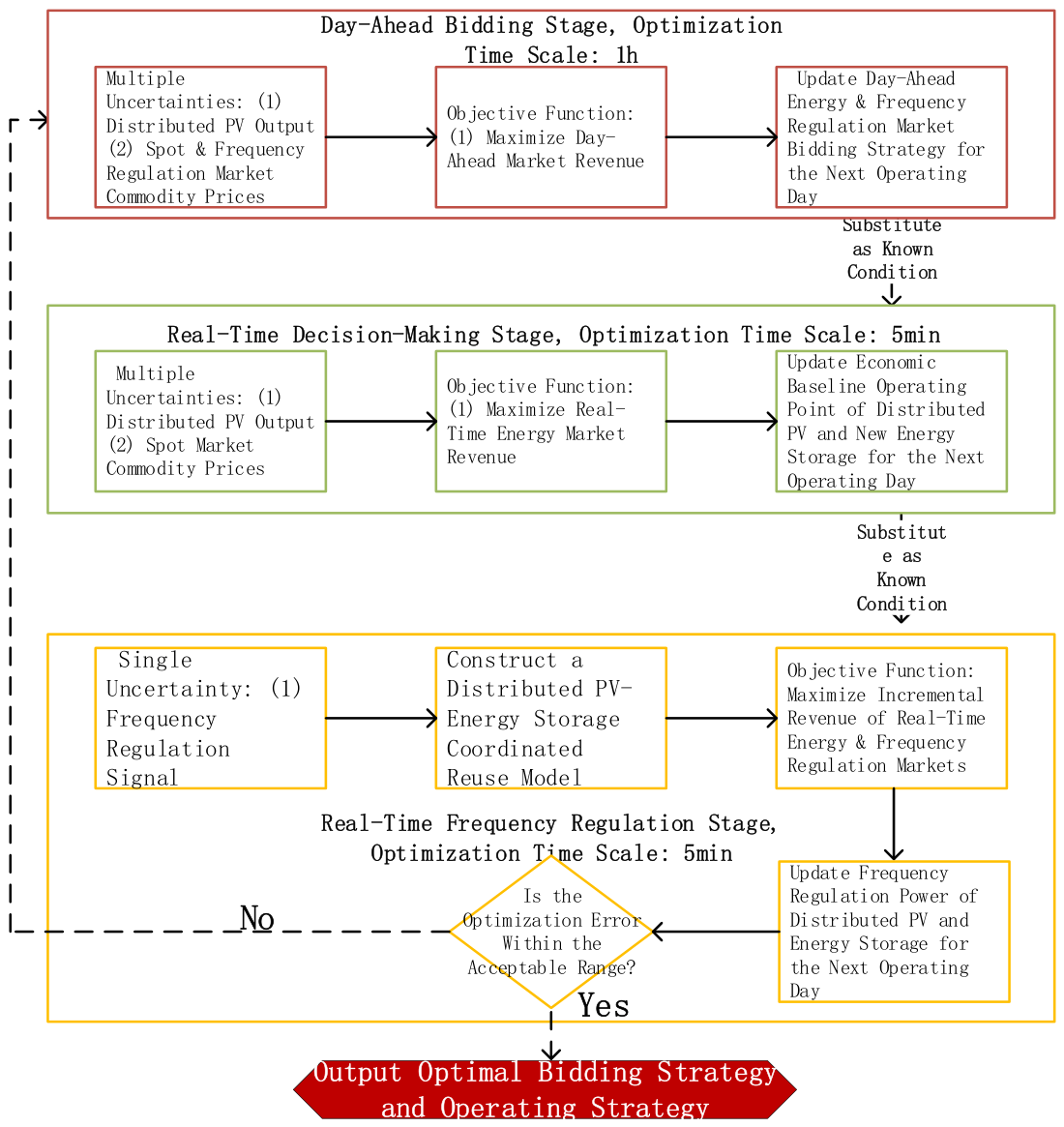
This paper adopted a multi-stage stochastic programming approach, designing the decision-making process of the PV-storage VPP participating in both the spot market and the frequency regulation market as a three-stage sequential framework, as illustrated in Figure 2. The first stage (day-ahead bidding) addresses the capacity allocation optimization problem; the second stage (real-time optimization) determines the baseline operating points of the resources (distributed PV and energy storage) managed by the PV-storage VPP agent; and the third stage (real-time frequency regulation) constructs a PV-storage coordinated multiplexing model to achieve optimal dual-market revenue through the dynamic adjustment of the regulation power. This segmented modeling strategy transforms the complex multi-time-scale, multi-market decision-making problem into a series of interrelated subproblems. Each stage is equipped with exclusive decision variables and a local objective function, ultimately achieving the global optimization of the PV-storage VPP’s total revenue through the following equation.
min R = E ( R 1 ( x 1 , δ 1 ) + E ( R 2 ( x 2 , δ 2 ) + E ( R 3 ( x 3 , δ 3 ) ) ) )
In the formula, R represents the total revenue of a PV-storage VPP participating in multiple markets; Ri (i = 1,2,3) is the objective function for each stage; x1, x2, and x3 are the optimization variables for each stage; δ1, δ2, and δ3 are the random parameters for each stage; and E(·) represents the expected value calculation for all possible outcomes of the random parameter for the terms within the parentheses. The specific models for each stage are explained in detail below.

2.2.1. Bidding Stage

The three-stage market decision optimization model constructed in this paper differs significantly from conventional multi-stage stochastic optimization problems. In this model, the coefficients of the first-stage model are not entirely based on deterministic information, but introduce uncertain factors such as day-ahead electricity and frequency regulation market prices. To ensure the feasibility of solving the model and meet the unexpected requirements of stochastic optimization problems, optimal estimation theory is used to process the model, and the mean of the overall estimation sample is used as the overall estimate value in the calculation. The process of obtaining the overall estimation sample includes the following steps: (1) Data collection stage: collect actual operating data of typical electricity markets, including day-ahead electricity market prices and frequency regulation market-capacity-clearing prices and performance-clearing prices at 5 min intervals. (2) Statistical analysis stage: calculate the volatility variance in each market price based on massive historical data. (3) Simulation generation stage: use the Monte Carlo simulation method to generate a large number of random deviations based on the volatility characteristics of each price, as the volatility components of the price sample. (4) Sample construction stage: select typical daily market prices as benchmark values, superimpose them with the random deviations generated by the simulation, and finally form a complete overall estimation sample.
Besides the day-ahead electricity and frequency regulation market prices, the actual output level of distributed photovoltaic power also exhibits uncertainty during the day-ahead bidding phase. To address this issue, this paper employed a modeling method similar to that used for the aforementioned market electricity prices: using the day-ahead forecast of the PV output as a benchmark, and generating prediction errors using a Monte Carlo simulation. Notably, this model also adopts this “benchmark value + random deviation” approach in the second stage, the “real-time optimization stage,” with each random deviation corresponding to a specific scenario.
A Monte Carlo simulation is used to generate uncertain scenarios of PV output and market prices, with 1000 original scenarios generated. To reduce the computational complexity of multi-stage stochastic optimization, the fast-forward selection method is adopted for scenario reduction. Typical scenarios are selected on the principle of the minimum probability distance, and 30 scenarios are finally retained. After reduction, the probability of each scenario is normalized and assigned the corresponding probability πs (s = 1, 2, …, 30), satisfying ∑πs = 1, and the probability distribution error is less than 5%. The probabilities of the 30 reduced scenarios range from 0.021 to 0.045 with a uniform distribution, which can fully characterize the stochastic fluctuation characteristics of market prices and the PV output. It greatly improves the solution efficiency while ensuring the integrity of random characteristics. The above scenario probabilities are used as the input conditions of the stochastic dual-dynamic-programming (SDDP) algorithm.
The current bidding stage model is as follows:
min x 1 R 1 ( x 1 , δ 1 ) = t = 1 T ( R t , d a , e + m M R t , m , d a , f r )
R t , d a , e = λ t , d a , e P t , d a , e
R t , m , d a , f r = λ t , m , c a p P t , m , d a , f r + λ t , m , p i P t , m , d a , f r
In the formulas, x1 ∈ {Pt,da,e, Pt,m,da,fr}; δ1 ∈ {λt,da,e, λt,m,cap, λt,m,pi}; Rt,da,e is the revenue of the PV-storage VPP in the day-ahead electricity market; Rt,m,da,fr is the revenue of the PV-storage VPP in the day-ahead frequency regulation market; λt,m,cap and λt,m,pi are the frequency regulation capacity and performance-clearing price in the day-ahead frequency regulation market (t, m) period, respectively; and Pt,m,da,fr is the winning bid amount of the PV-storage VPP in the day-ahead frequency regulation market (t, m) period.
The constraints at the current bidding stage include:
(1) The total upper limit constraint on the bidding capacity
P t , d a , e + P t , m , d a , f r P r a t e d , p v + P d i s , m a x
P t , d a , e + P t , m , d a , f r P c h , m a x
In the formulas, Prated,pv is the rated installed capacity of the distributed photovoltaic power, and Pdis,max and Pch,max are the maximum values of the energy storage charging and discharging power, respectively.
(2) The maximum capacity constraint for frequency modulation bidding
In the context of the electricity market, considering the inherent volatility of photovoltaic power output, in order to ensure the actual implementation effect of frequency regulation services, it is clearly required that the frequency regulation capacity declared by new energy entities must simultaneously meet the following requirements: not exceeding 24% of their rated capacity; and not exceeding their maximum ramp power within 5 min.
P t , m , d a , f r P d i s , m a x + min ( 24 % P r a t e d , p v , 5 μ r a m p P r a t e d , p v )
P t , m , d a , f r 0
In the formulas, μramp is the power ramp-up rate per unit minute for distributed photovoltaic power.

2.2.2. Real-Time Optimization Phase

In the real-time optimization phase, the main task is to determine the baseline economic operating point for distributed photovoltaic and energy storage systems. This baseline serves a dual purpose: providing guidance for the real-time operation of PV and energy storage, and acting as a reference standard for evaluating their frequency regulation capabilities. During the day-ahead bidding phase, PV-storage VPPs participate in market bidding as market players; therefore, only their total bid volume needs optimization. When entering the real-time optimization and real-time frequency regulation phase, although the market revenue still needs to be calculated from an overall perspective, to ensure that the actual operation of each resource conforms to physical constraints, both need to be modeled and analyzed separately as independent entities. It is important to emphasize that this separate treatment does not affect their collaborative relationship.
When the time comes for the real-time optimization stage, the price information of the day-ahead electricity market is clarified, and the declared electricity volume of the relevant market is confirmed. At this stage, the main uncertainties that decision-makers need to deal with are the fluctuations in real-time electricity prices and the changes in distributed photovoltaic power generation. For these two random variables, the modeling method of “baseline value combined with random quantity” proposed above is used. It is worth noting that, as the actual operation time approaches, the accuracy of the photovoltaic power generation prediction will be significantly improved. In practice, photovoltaic power generation prediction is usually updated in the intraday stage before real-time operation, and the prediction time scale is increased to the 5 min level. Therefore, in the real-time optimization process, the base value of photovoltaic power generation can use the latest prediction data, and the value of the random quantity representing the prediction deviation will also be reduced accordingly.
The objective function for the real-time optimization phase using a dual-settlement model is as follows:
min x 2 R 2 ( x 2 , δ 2 ) = t = 1 T m M λ t , m , r t , e P t , m , r t , e P t , d a , e
P t , m , r t , e = P t , m , r t , p v + P t , m , r t , e s
In the formulas, x2 ∈ { Pt,m,rt,pv, Pt,m,rt,es}; δ2 ∈ {λt,m,rt,e}; the bidding volume of distributed photovoltaic (t, m) in the real-time electricity market is Pt,m,rt,pv; and the bidding volume of energy storage (t, m) in the real-time electricity market is Pt,m,rt,es.
The constraints are as follows:
(1) Constraints of distributed photovoltaic power
P t , m , r t , p v P r a t e d , p v
(2) Energy storage constraints
P t , m , r t , e s P d i s , m a x
P t , m , r t , e s P c h , m a x
S m i n E r a t e d , e s E t , m S m a x E r a t e d , e s
E t , m = E t , m Δ m Δ E t , m
Δ E t , m = η es ( P t , m , r t , e s ) Δ t
E 23 , 12 = E 0 , 0
In the formulas, Et,m is the electrical energy stored in the time period (t, m); Erated,es is the rated capacity of the energy storage; Smin and Smax are the minimum and maximum states of charge of the energy storage, respectively; and ηes is the energy storage charging and discharging efficiency.
(3) Market bidding constraints
Market regulations are established by market management to avoid excessive differences between the real-time bidding volume and the day-to-day bidding volume.
P t , m , r t , e ψ P t , d a , e P t , d a , e 0 ψ P t , m , r t , e ψ P t , d a , e = 0 P t , m , r t , e ψ P t , d a , e P t , d a , e < 0
In the formula, Ψ is the difference coefficient between real-time bidding and day-ahead bidding, which is determined by the market.

2.2.3. Real-Time Frequency Modulation Stage

In the photovoltaic-storage collaborative reuse model constructed during the real-time frequency modulation stage, the frequency modulation power, as a key factor in cross-market revenue coordination, is the core optimization variable of the model. By dynamically optimizing the frequency modulation power curve, the overall revenue of the electricity market and the frequency modulation market can be maximized.
1. Photovoltaic-storage collaborative reuse model
The photovoltaic-storage collaborative reuse model consists of two parts: the real-time energy market revenue Rt,m,rt,e of the PV-storage VPP during the time period (t, m) and the frequency regulation market revenue Rt,m,fr, as shown below:
R m u l t i = max t = 1 T m M R t , m , r t , e + R t , m , f r
In the formula, Rmulti represents the total real-time market revenue.
(1) Real-time electricity market revenue Rt,m,rt,e
In the model constructed in this section, the total revenue of a PV-storage VPP participating in the real-time electricity market can be decomposed into two components: basic revenue and additional revenue. Basic revenue depends on the product of the bidding volume of the PV-storage VPP and the real-time market-clearing price; this portion of revenue is determined before the frequency regulation decision and is immutable. To simplify the calculation process, the model’s objective function only retains the additional revenue term directly related to the frequency regulation power; its specific quantification method is shown in Equation (28).
R t , m , r t , e = λ t , m , r t , e k K P t , m , k , f r Δ k
In the formula, kK, K = {Δk, 2Δk, …, 75Δk} and Δk = 4 s, used to characterize the response frequency of the PV-storage VPP to the frequency modulation signal; Pt,m,k,fr,res is the frequency modulation power of the PV-storage VPP at time (t, m, k). When Pt,m,k,fr,res > 0, the PV-storage VPP discharge provides an up-frequency modulation auxiliary service, and when Pt,m,k,fr,res < 0, the PV-storage VPP charging provides a down-frequency modulation auxiliary service.
(2) Frequency modulation market revenue Rt,m,fr
Due to the characteristics of a fast response and flexible regulation of energy storage systems, PV-storage VPPs can achieve near-perfect scores in both delay and correlation indicators when providing frequency regulation services. Based on this, to simplify the model calculation, this paper only considers the contribution of the accuracy score to the overall frequency regulation performance. Specifically, in Equation (8), let a = b = 0 and c = 1. Under this condition, the revenue of the PV-storage VPP in the frequency regulation market and the corresponding frequency regulation performance score are quantified by Equations (29) and (30), respectively.
R t , m , f r = M t , m , p e r P t , m , f r ( λ t , m , c a p + r f r λ t , m , p i )
M t , m , p e r = 1 1 75 k K P t , m , k , f r , r e q + P t , m , k , f r , r e s P t , m , f r
In the formulas, Pt,m,k,fr,req is the frequency modulation demand received by the optical storage VPP at time (t, m, k).
P t , m , k , f r , r e q = ζ t , m , k P t , m , fr
In the formula, ζt,m,k is the frequency-modulated signal received by the optical storage VPP at time t, m, k.
Directly utilizing Equation (30) to calculate the frequency regulation market revenue poses significant computational challenges. First, Equation (30) involves absolute value operations, rendering the objective function non-linear. Although well-established linearization techniques can handle absolute values, such methods substantially increase the constraint size of the model, thereby reducing the computational efficiency. Second, adopting a 4 s optimization time step results in an extremely high computational complexity—even for a single-day scheduling horizon, the number of decision variables exceeds 21,600, seriously affecting the solution feasibility.
To address these challenges, this paper proposes simplifying the revenue model by extending the optimization time scale of the frequency regulation stage from 4 s to 5 min. On the one hand, the frequency regulation performance score itself is calculated based on the average value of the regulation accuracy within 5 min intervals; thus, relaxing to this time scale does not affect its evaluation basis. On the other hand, the additional revenue in the energy market is determined solely by the total integral over the 5 min scheduling period and is independent of second-level instantaneous power fluctuations. Therefore, extending the optimization scale to 5 min effectively reduces the number of decision variables and significantly improves the model solvability while preserving the problem’s essence and modeling accuracy.
To resolve the absolute value operation in Equation (29) while aligning with the characteristics of the frequency regulation performance score function, a non-negative intermediate decision variable Pt,m,mid,fr is introduced. The performance score function is characterized by the following property: when the regulation power fully meets the demand (i.e., Pt,m,k,fr,res = −Pt,m,k,fr,req), the performance score equals 1, achieving the optimal value; as the actual power deviates from the demand, the performance score decreases.
P t , m , f r , r e s = r t , m P t , m , m i d , f r
As shown in Equation (32), the time scale of the optimization problem was converted to 5 min. Here, Pt,m,fr,res represents the total frequency regulation power of the PV-storage VPP during interval (t,m), reflecting its overall performance, whereas −rt,m denotes the typical frequency regulation signal during interval (t,m), reflecting the system’s overall demand.
The introduction of the constraint Pt,m,mid,fr ≥ 0 aims to exempt the model from absolute value operations. As indicated in Equation (32), this constraint ensures that the regulation power Pt,m,fr,res is opposite in direction to the signal −rt,m, thereby guaranteeing that the service provided by the PV-storage VPP aligns with system requirements. The practical basis for this constraint is the widespread performance threshold in frequency regulation markets; if the direction is inconsistent, the performance score is inevitably below the threshold, which is not permitted in this model. Consequently, the introduction of the intermediate variable simultaneously addresses two major issues: model linearization and market compliance.
After the aforementioned simplifications, the real-time energy market revenue model Rt,m,rt,e is transformed into Equation (33), and the frequency regulation market revenue model Rt,m,fr is transformed into Equation (34).
R t , m , r t , e = λ t , m , r t , e P t , m , f r , r e s Δ t
R t , m , f r = [ P t , m , f r r t , m ( P t , m , f r P t , m , m i d , f r ) ] ( λ t , m , c a p + r f r λ t , m , p i )
2. Constraints
The mathematical model established for the reuse problem of photovoltaic-storage synergy considers the following constraints.
(1) Distributed photovoltaic power output constraints
0 P t , m , r t , p v + P t , m , f r , p v P t , m , s j , p v
P t , m , r t , p v 0
In the formulas, Pt,m,fr,pv is the frequency modulation power of photovoltaic power during the time period (t, m); Pt,m,sj,pv is the actual output of photovoltaic power during the time period (t, m).
(2) Energy storage operation constraints
P t , m , r t , e s + P t , m , f r , e s P d i s , m a x
P t , m , r t , e s P t , m , f r , e s P c h , m a x
S m i n E r a t e d , e s E t , m S m a x E r a t e d , e s
Δ E t , m = η e s ( P t , m , r t , e s + P t , m , f r , e s ) Δ t
E t , m = E t , m Δ m Δ E t , m
E 23 , 12 = E 0 , 0
In the formulas, Pt,m,fr,es is the frequency regulation power of energy storage during the time period (t, m).
(3) Operational constraints of PV-storage VPP equipment
P t , m , f r , r e s = P t , m , f r , p v + P t , m , f r , e s
(4) Frequency modulation power upper limit constraint
P t , m , f r , r e s P t , m , f r
(5) Other constraints
0 P t , m , m i d , f r P t , m , f r , r e s
3. Objective function
The frequency modulation market revenue model in the reuse model constructed in the preceding section needs to be adjusted in conjunction with the objective function of the model in the day-ahead bidding stage: in the day-ahead stage, the frequency modulation performance score is preset to 1, so the model only needs to focus on the deviation between the actual score and this preset value. Let ΔMt,m,per = Mt,m,per-1 represent the revenue. Then, the specific form of the objective function for the third stage is as follows:
min x 3 R 3 ( x 3 , δ 3 ) = t = 1 T m M ( Δ R t , m , r t , e + Δ R t , m , f r )
In the formula, x3∈{Pt,m,fr,res, Pt,m,mid,fr}; δ3 ∈ {−rt,m}; and ΔRt,m,rt,e and ΔRt,m,fr correspond to the incremental revenue of the PV-storage VPP in the electricity market and its revenue deviation in the frequency regulation market, respectively, and are calculated as follows:
Δ R t , m , r t , e = λ t , m , r t , e P t , m , f r , r e s Δ t
Δ R t , m , f r = Δ M t , m , p e r P t , m , f r ( λ t , m , c a p + r f r λ t , m , p i ) = P t , m , f r r t , m ( P t , m , m i d , f r P t , m , f r 1 ) [ λ t , m , c a p + r f r λ t , m , p i ]
The constraints are the same as those in Equations (35)–(46).

2.2.4. Model Solving

Pereira and Pinto et al. proposed that the stochastic dual-dynamic-programming algorithm is currently an effective tool for solving multi-stage stochastic optimization problems. Based on the stochastic dual-dynamic-programming algorithm, the three-stage stochastic optimization model for the optical-storage VPP constructed in this section can be simplified as follows:
f 1 = E ( R 1 ( x 1 , δ 1 ) + z 2 ) s . t .         A 1 x 1 b 1
f 2 = E ( R 2 ( x 2 , δ 2 ) + z 3 ) s . t .         A 2 x 2 b 2 B 1 x 1
f 3 = E ( R 3 ( x 3 , δ 3 ) ) s . t .         A 3 x 3 b 3 B 2 x 2
In the formulas, z2 and z3 are defined as subproblems of the first and second stages, used to evaluate the expected returns of subsequent stages; Aⱼ(j = 1, 2, 3) and Bⱼ(j = 1, 2, 3) are the coefficient matrices of the corresponding stages; bⱼ(j = 1, 2, 3) is the resource vector of the corresponding stage; and fⱼ(j = 1, 2, 3) is defined as the cumulative return from the j-th stage to the final stage. Therefore, f1 is the global total return. The above algorithm can be used to effectively solve this three-stage stochastic optimization problem.

3. Revenue Distribution Model for Photovoltaic-Storage VPP Collaborative Reuse

3.1. PV-Storage VPP Based on Stakeholder Division

Section 2 of this paper, especially Section 2.1 and Section 2.2, focuses on the market decision-making and operational optimization problems when distributed photovoltaics and energy storage jointly participate in the electricity market. At the decision-making planning level, the PV-storage VPP is treated as a unified entity to study its external trading behavior in the electricity market; at the operational optimization level, PV and energy storage are modeled and analyzed separately to satisfy actual physical operation constraints. However, to maximize the overall revenue and fairly distribute cooperative benefits, it is necessary to partition the internal benefit structure of the PV-storage VPP.
To this end, this paper proposes a benefit-partitioning method based on investment entities. Considering that large-scale distributed PV and energy storage may belong to different or the same investors, to adhere to the principle of “whoever invests benefits” and clarify the benefit allocation path, PV or energy storage belonging to the same investor can be aggregated at the benefit level (they remain independent in actual operation and jointly participate in the cooperative game). By quantifying the contribution degree of each investment entity to the total revenue, the share of revenue it deserves is calculated. In other words, the PV-storage VPP studied in this paper can be regarded as consisting of several virtual sub-coalitions, each linked by an investment entity, with one investment entity corresponding to one sub-coalition. This sub-coalition serves merely as a benefit allocation unit and does not involve an additional cooperative game process internally.
According to the differences in investment composition, this paper classifies the investment entities under the PV-storage VPP into three categories, as shown in Table 1: Type 1 invests only in distributed PV, Type 2 invests only in energy storage, and Type 3 invests in both distributed PV and energy storage. The number of PV or energy-storage devices included in each type is unrestricted.

3.2. Nash–Harsanyi Bargaining Game Theory

Based on Nash–Harsanyi negotiation game theory, this paper constructs a profit distribution model applicable to the various investment entities within a PV-storage VPP. Assume that all investment entities included in the PV-storage VPP constitute a set N = {1, 2,…, n}, and let SN represent any sub-alliance within it. Let v(N) represent the total market profit of the PV-storage VPP as a whole. If the function v(·) satisfies v(ω) ≠ 0, then it is called the characteristic function. This game model must satisfy the following three basic principles: individual rationality, overall rationality, and alliance rationality, as shown in Equations (53)–(55), respectively.
ω i ν { i } i = 1 ,   2 ,   ,   n
i N ω i = ν N
i S ω i ν ( S )
In the formulas, ωi represents the i-th investment entity, or the allocated income.
Based on the aforementioned cooperative game theory, Nash–Harsanyi proposed a model for solving the profit distribution scheme, as shown in Equation (56).
φ i * = arg max i N U φ i U φ i , min α i
where φi denotes the revenue allocation ratio corresponding to investment entity i. φi ∈ (0, 1) is a decision variable of the model and satisfies i = 1 n φ i = 1 to conform to the principle of group rationality. The argmax(⋅) function represents the value of the decision variable when the function inside the parentheses attains its maximum value. U(⋅) is the utility function of the model, which can reflect the risk preferences of different investment entities; αi is the bargaining power of investment entity i, which is an overall consideration of its contribution within the coalition and serves as the core factor determining the weight of the revenue allocated to that entity, satisfying i = 1 n α i = 1 ; and φi,min is the initial bargaining value of investment entity i.

3.3. Profit Distribution Model Oriented Towards Investors

As described in Section 2.2, the model 56 consists of a utility function, negotiating power, and initial negotiation values. This section will build upon the multi-stage stochastic optimization operation strategy for the PV-storage VPP constructed in Section 2.2, and specifically model these three elements to achieve an optimal distribution mechanism for PV-storage VPP returns based on the actual contributions of each investment entity.

3.3.1. Utility Function

According to the Nash–Harsanyi negotiation theory, utility functions reflect the risk preferences of game participants. Their curves vary in shape, but all satisfy the condition that the domain and range are within the range [0, 1] and are monotonically increasing. In existing research, a logarithmic form of the utility function is widely used, as shown in Equation (57).
U i ( φ i ) = ρ 1 + ρ 2 l n φ i + ζ i 2 1 2 ζ i , w h e n   ζ i < 0.5 φ i , w h e n   ζ i = 0.5 1 ρ 1 + ρ 2 l n 1 φ i + 1 ζ i 2 1 2 1 ζ i , w h e n   ζ i > 0.5
In the formula, ζi∈(0,1) is the risk preference coefficient of investor i. ζi = 0.5 indicates that investor i is risk-neutral, and its utility function is a direct proportional function; ζi < 0.5 indicates that investor i is a risk-averse investor, and its utility function is a transformation of a logarithmic function; and ζi > 0.5 indicates that investor i is an adventurer, and the concavity and convexity of its utility function changes compared to that of a risk-averse investor. By introducing a risk preference coefficient, the utility function effectively distinguishes the risk attitudes of different investment entities, thereby characterizing the individual characteristics of participants in the game. ρ1 and ρ2 are two parameters to be determined. Once the risk preference coefficient is given, the system of two linear equations in two variables can be solved by substituting the boundary points (0,0) and (1,1).

3.3.2. Negotiation Power

Negotiation power is a key indicator for measuring the contribution of each investment entity to the overall alliance and a decisive factor affecting its final profit distribution ratio. Generally, the stronger the negotiating power of an entity, the higher its share of profit distribution. Based on the multi-stage stochastic optimization operation model of the PV-storage VPP established in Section 2.2, this paper selects the following four dimensions of factors to model and analyze the negotiating power of each investment entity.
(1) Marginal contribution rate
From the perspective of economic returns, the marginal contribution rate reflects the degree to which each investment entity contributes to the overall market returns of the alliance, and its calculation formula is as follows:
B i M C = ν ( N ) ν ( N { i } ) ν ( N )
In the formula, Bi,MC∈(0,1) represents the normalized marginal contribution rate of investment entity i. v(N − {i}) represents the market returns of the remaining alliance members after investor i withdraws from the alliance.
(2) Prediction accuracy of distributed photovoltaic power generation
This paper focuses on a PV-storage VPP composed of large-scale distributed photovoltaics and energy storage. The output prediction errors between different photovoltaic units may cancel each other out due to their opposite directions, making it difficult to directly characterize the overall prediction error using the error of a single photovoltaic unit. To address this, this paper proposes a photovoltaic prediction error measurement method that considers the difference in error direction, as shown in Equation (59).
e i F A = 1 24 ( t , m ) T × M Y | P i , t , m o u t , r t P i , t , m f o r e , r t | P i , t , m o u t , r t
In the formula, ei,FA represents the output prediction deviation of investment entity i under the directional difference measurement method, and P(·)out,rt and P(·)fore,rt represent the actual output and intraday output prediction values of distributed photovoltaic power, respectively. It is a dual-valued constant reflecting directional difference; when the prediction deviation direction of a certain distributed photovoltaic power is consistent with the overall deviation direction, Y > 1; otherwise, Y < 1.
The main idea behind the aforementioned directional difference measurement method is as follows: when the prediction deviation direction of a distributed photovoltaic (PV) system is the same as the overall deviation direction of the consortium, it indicates that the deviation amplifies the overall error, and therefore it is amplified by multiplying by a coefficient greater than 1. Conversely, if its direction is opposite to the overall deviation, it means that the deviation has a certain offsetting effect on the overall error, and therefore, it is reduced by multiplying by a coefficient less than 1. This method not only considers the absolute value of the prediction deviation, but also integrates the influence of the deviation direction on the overall error, thus better aligning with the actual research scenario of large-scale PV-storage VPPs participating in the electricity market.
Based on Equation (59), the photovoltaic prediction accuracy score Bi,FA of investment entity i is calculated as follows:
B i F A = min i e i F A e i F A
The above formula can make the prediction accuracy score fall within the [0, 1] interval, and satisfy the condition that the subject with the larger prediction error has a lower score.
(3) Energy storage capacity
The energy storage capacity provides ample bidding space and effective decision support for PV-storage VPPs. The larger the energy storage capacity, the more beneficial it is for operation. Therefore, the formula for calculating the energy storage capacity score is as follows:
B i C P = P R , i S max i P R , i S
In the formula, BiCP represents the energy storage capacity score of investment entity i, which also falls within the range of [0, 1].
(4) Energy storage utilization rate
In analyzing the decision-making process of photovoltaic-storage collaborative participation in market transactions, this study focused on optimizing economic benefits and did not factor in the performance degradation costs caused by frequent charging and discharging of energy storage systems. Energy storage batteries experience irreversible capacity degradation during repeated or deep charging and discharging, significantly impacting their lifecycle operational economics. Therefore, when distributing revenue within the cooperative alliance, energy storage devices can receive corresponding compensation based on their actual charging and discharging depth during operation. It is reported that long-term field data from 85 photovoltaic plants in Central Europe showed that the actual service life of PV panels is only about 10–12 years, nearly half of the designed 20–25 years. Severe failures rise rapidly after 10 years of operation, which greatly increases the maintenance costs and affects the actual economic benefits of PV systems [18]. To quantify this impact, this study converted the lifespan loss of energy storage devices into additional operating costs corresponding to unit charging and discharging power, as shown in Equation (62).
e i U R = ( t , m ) T × M P i , t , m , r t , e s + P i , t , m , f r , e s Δ t 24 E i , r a t e d , e s
In the formula, ei,UR represents the operating cost of investment entity i due to energy storage charging and discharging. Then, it is converted into an energy storage utilization score Bi,UR within the interval [0, 1] using Equation (63):
B i U R = e i U R max i e i U R
The four factors mentioned above affect the negotiating power of the three types of investment entities to varying degrees. The formulas for calculating the negotiating power of different types of investment entities are as follows:
B i = λ B i M C + μ B i F A , i type   1 λ B i M C + μ p B i C P + q B i U R , i type   2 λ B i M C + μ a B i F A + b B i C P + c B i U R , i type   3
In the formula, Bi represents the negotiating power of investment entity i before normalization, and λ, u, p, q, a, b, c are all weighting coefficients, satisfying the following constraints:
λ + μ = 1 p + q = 1 a + b + c = 1
Finally, to ensure that the sum of the negotiating power of all investors is 1, their respective negotiating power values need to be normalized, as shown in Equation (14).
α i = B i i B i
At this point, the negotiating power of each investment entity has been calculated.

3.3.3. Initial Point of Negotiation

The initial negotiation point represents the minimum allocation ratio that the investor can accept, which can be solved using the principle of individual rationality.
φ i , min = v i ν ( N )
In the formula, vi represents the revenue of investment entity i when operating alone. Among them, entity type one invests only in distributed photovoltaics, and its model for operating alone is the same as the distributed photovoltaic-independent operation model introduced in the previous section. Entity type two invests only in energy storage, and its model for operating alone is the same as the energy-storage-independent operation model introduced in the previous section. Entity type three can be regarded as a small-scale photovoltaic-energy storage VPP, and its market revenue when operating alone is still solved using the three-stage reuse model proposed in this paper.

4. Case Analysis

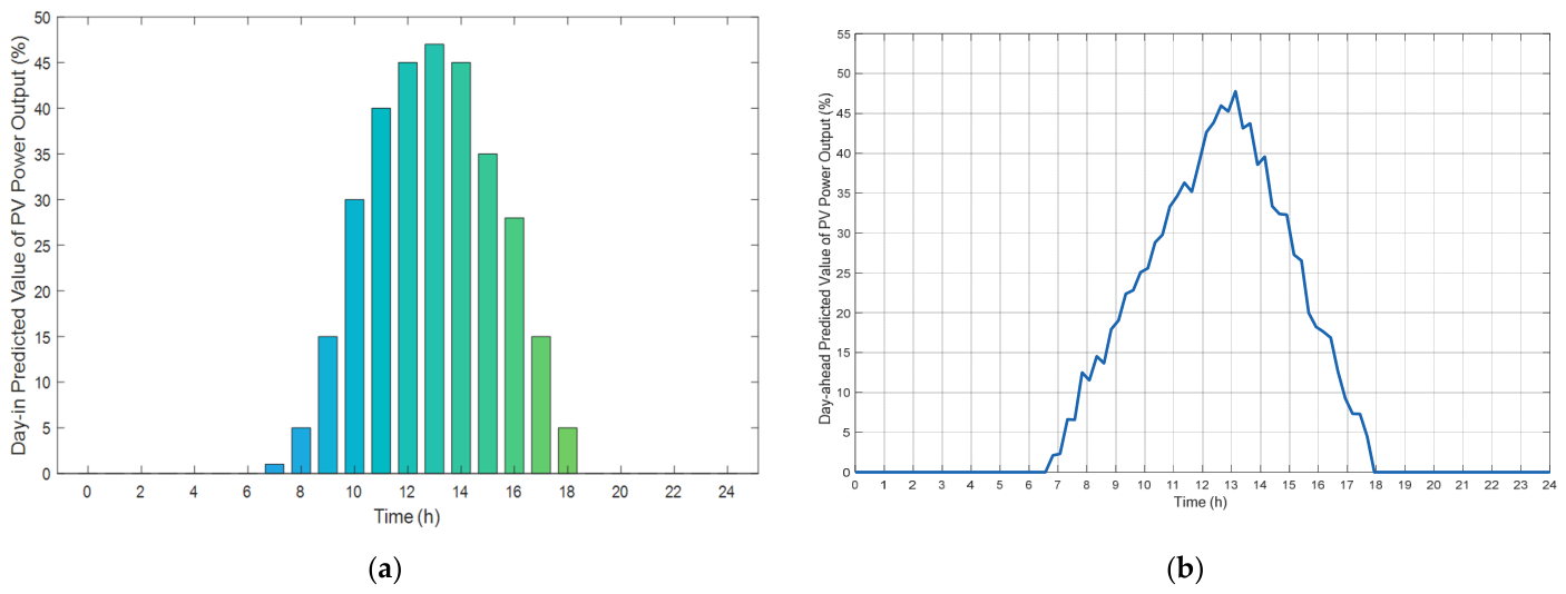
In the photovoltaic VPP constructed in this example, 120 MW of photovoltaic power was connected, the total power of the energy storage system was 20 MW, and the total capacity was 40 MWh. The comprehensive charge and discharge efficiency of the energy storage unit was 0.81, the upper limit of the allowable operating range of its charging state was 100%, and the lower limit was 5%. The maximum climb rate of the photovoltaic output force in the minute level was set to 8%, and the overall output force prediction curve of the distributed photovoltaic is shown in Figure 3.
The statistics showed that the average error of the distributed photovoltaics’ daily forecasts was 22%, and the average error of the intraday forecasts was 12% [19]. The standard deviation of the photovoltaic output random variable was set based on the above error values, and a Monte Carlo simulation method was used to generate a large number of photovoltaic output random scenarios required for optimization. At the same time, the actual clearing price data of the electricity market on a certain day was selected as the benchmark value of each electricity price random variable, and the electricity price scenario was constructed by superimposing the corresponding price fluctuation amount. Among them, the standard deviations of price fluctuations in the day-ahead electricity market, real-time electricity market and FM market were set at 6.056, 11.510 and 2.401, respectively. In this example, 1000 initial scenarios were generated by the Monte Carlo simulation, and 20 typical scenarios were retained after scenario reduction for the optimization calculation. The proposed three-stage stochastic optimization model was built based on stochastic programming theory and characterized uncertainties via the Monte Carlo simulation, which ensured its robustness against PV output fluctuations and market price changes. The inherent nature of the stochastic optimization method guarantees the model’s decision-making effectiveness even under large-fluctuation scenarios. In addition, the allowable deviation coefficient between the real-time and day-ahead market bidding volume stipulated in the market rules was 150%.

4.1. Market Decision Optimization Results

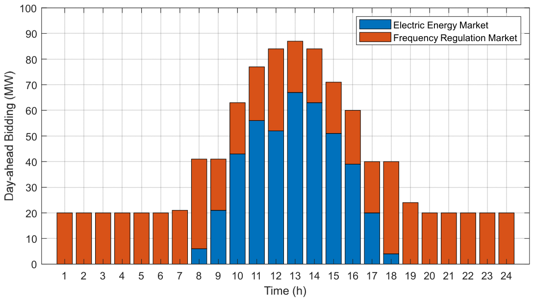
The results of the day-ahead market optimization bidding shown in Figure 4 show that the sum of the declared quantities of the photovoltaic VPP in the electric energy market (orange column) and the FM market (blue column) never exceeded its maximum dispatchable capacity. Since only hourly output forecasts for photovoltaics can be obtained during the decision-making stage, and the electricity market is declared on an hourly basis, in order to fully utilize capacity resources, the system adopts a strategy of equal declaration for 5 min periods within each hour in the FM market. Therefore, only bidding data for 24 periods are presented in the figure. The analysis showed that the system was actually operated independently by energy storage during the night light-free period, and it put all 20 MW of power into the FM market to obtain auxiliary service benefits; during the daytime period, it still maintained 15. The FM declaration volume of 35 MW shows that the performance-based pay-for-FM mechanism can form effective incentives. In the electricity market, the bidding volume is closely related to the photovoltaic output forecasts, reflecting the way in which the value of photovoltaic power generation is realized. The intervention of energy storage enables the system to dynamically optimize the configuration between electricity sales and FM services based on multiple market price signals, thereby significantly improving its operational flexibility and decision-making autonomy in the market environment.
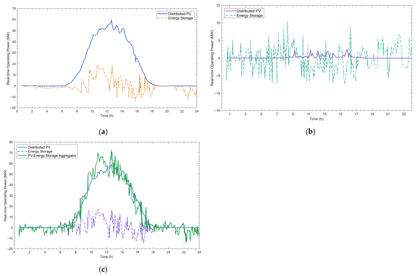
The optimization results of the second and third stages are shown in Figure 5.
For the distributed photovoltaic entities participating in the transaction, the results of their baseline operating point optimization in the second phase generally followed the changing trend of the intraday forecast output curve, aiming to ensure the expected returns of the electricity energy transaction as much as possible. The final actual operating curve is dynamically adjusted based on the real-time available output of photovoltaics and the overall frequency modulation demand of the system, striving to achieve synergy between reducing abandoned light and meeting frequency modulation requirements. The optimization results showed that the actual power generation capacity of the distributed photovoltaics was fully utilized and the overall system abandonment rate was close to zero. Further analysis of the optimization results of real-time FM power in the third stage showed that the distributed photovoltaics’ participation in FM was mainly concentrated in the periods when their output was relatively abundant, and in most cases, they provided FM services, thereby supporting the stability of system frequency while also promoting the maximum consumption of renewable energy.
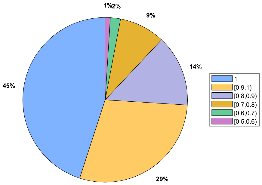
When photovoltaic VPPs participate in multiple markets, the frequency modulation task is mainly undertaken by energy storage units. Although the FM capacity declared a few days ago reached 15–35 MW, the actual FM power provided by the system mostly does not exceed 10 MW. In addition to the impact of the FM signal strength, another key reason for this phenomenon is that, under the revenue-oriented collaborative optimization model, the optical storage VPP aims to maximize the overall market revenue, and its operating strategy does not fully follow the FM signal. Figure 6 shows the FM performance score distribution of the optimized system in each time period. It can be seen that, during about 45% of the target day, the system tracks FM signals to obtain market returns, and in more than half of the remaining periods, its FM performance score is lower than 1, indicating that the system has actively reduced the FM tracking accuracy in order to improve the overall economy. This result verifies the effectiveness of the collaborative model proposed in this paper in expanding the revenue space of photovoltaic VPPs. It is worth noting that the FM performance score of the system was higher than 0.4 at all times of the day, meeting the minimum performance requirements for market access, demonstrating that the model is both economical and feasible.

4.2. Comparative Analysis of Market Returns Under Different Models

In order to verify the effectiveness of the constructed three-stage optimization model in improving the market returns of photovoltaic-storage VPP participation, this paper compared and analyzed its optimization results with three other typical models. The benchmark model adopted the three-stage model proposed in this paper for the collaboration of energy arbitrage and FM services. The comparison models were: an independent operation model (model I), an absolute FM model (model II) and a sequential optimization model (model III).
The photovoltaic VPP market return values obtained by each model are shown in Table 2.
As can be seen from the data in the table, the proposed basic model can help photovoltaic VPPs to improve market returns to varying degrees. First, the basic model combines distributed photovoltaics and energy storage, enhancing their profit space in market competition through the synergistic and complementary advantages between the two. Secondly, the optimization results confirm that, in the context of market reuse, the behavior of fully responding to FM signals is not the most profitable. Using price signals and the analog-optimized FM power of FM signals can achieve a profit increase, with a single-day profit increase percentage of about 5%. Finally, sequential optimization methods sacrifice model accuracy and make it difficult to achieve repeated updates and adjustments to market decisions. Therefore, only suboptimal solutions can be obtained.

4.3. Results of the Division of Investment Entities

The investment entities were divided into 120 MW distributed photovoltaic and 20 MW/40 MWh energy storage selected for the example, and the results are shown in Table 3.
According to the information in the table, the photovoltaic-storage VPP in this example consisted of five participating entities with different investment types. Specifically, entities A and B belonged to type 1, which only invests in distributed photovoltaics, and their risk appetite coefficient was set at 0.6; entity C was type 2, which only invests in energy storage and is risk-neutral; and entities D and E belonged to type 3, which invests in both photovoltaics and energy storage and shows a stronger risk-taking tendency than the other entities; its risk appetite coefficient is 0.7. The day-ahead and intraday forecast error data corresponding to each distributed photovoltaic unit are shown in Table 4.

4.4. Benefit Allocation Calculation Results

Based on the optimization results in Section 3.2, the three-stage stochastic optimization model built in this paper was used to calculate that the total return of the photovoltaic-storage system on the target date was 15,605.25 yuan. The following will use the return distribution model established in Section 3.3 to distribute this total return among various investment entities.
After determining the risk appetite coefficient of each investment entity, a corresponding utility function can be established, the specific form of which is shown in Table 5. Since the constraint φi is incorporated in the calculation ∈ (0,1), the function expression is simplified and the form after absolute value removal is shown in the table. The results of the calculation of the negotiation power and negotiation baseline values are listed in Table 6. Among them are the negotiation force weight coefficient, λ, μ, p, q, a, and b. The values of c are 0.6, 0.4, 0.5, 0.5, 0.4, 0.3, and 0.3, respectively.
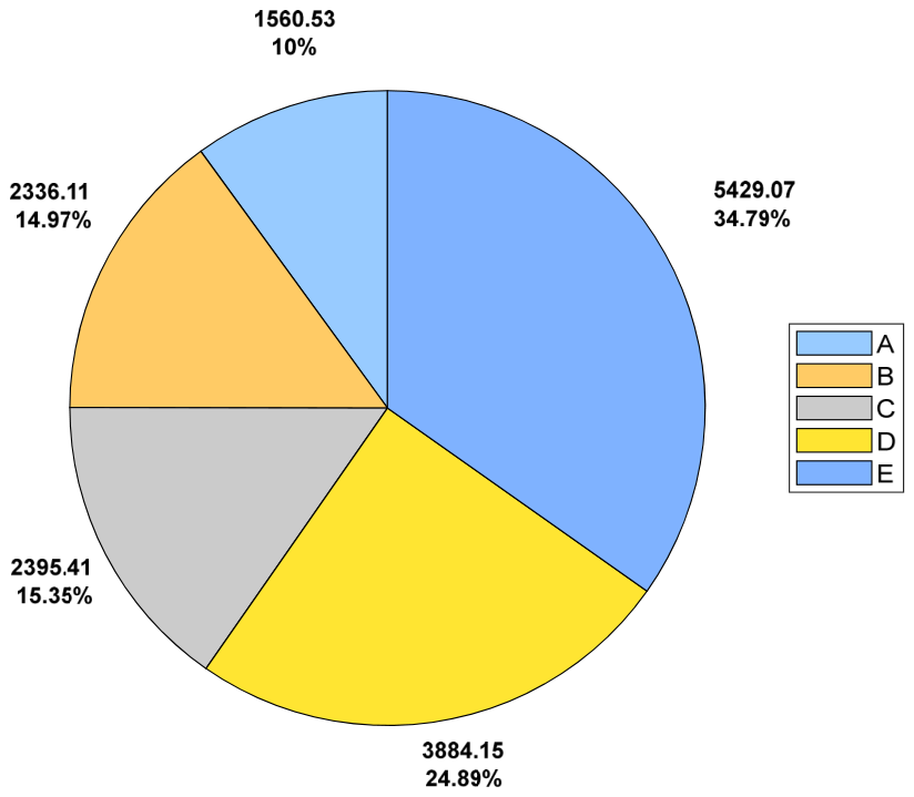
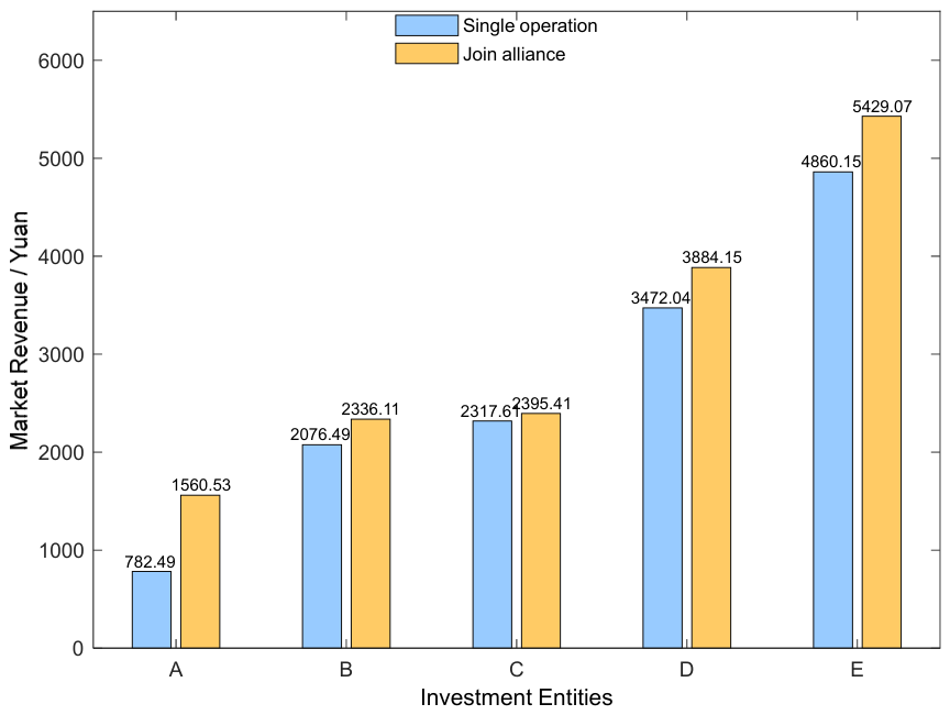
By substituting the above parameters into the formula, the profit ratio and profit value of each investment entity can be found, as shown in Figure 7. Further, Figure 8 shows the difference between the distributed benefits obtained by each entity after participating in the photovoltaic-storage VPP cooperation and the benefits that it can obtain when operating independently.
According to the allocation results in Figure 7, although investment entity B had three times the installed photovoltaic capacity of entity A, due to its large photovoltaic forecast error, the forecast accuracy score was only half of A, resulting in a relatively low negotiation power, and the final profit distribution ratio was only about 50% higher than A. Investment entity C, because of its single composition and limited size, had the lowest marginal contribution to the union as a whole. Investment entities D and E belonged to type III, whose small-scale optical storage systems achieved a relatively high share of revenue distribution in the alliance due to their good cooperative operation characteristics.
As can be seen from Figure 8, after participating in the photovoltaic-storage VPP cooperation, the market returns of each investment entity increased. Among them, investment entity A benefited from its high photovoltaic output prediction accuracy, and its profit growth reached 99.43%, the highest among the five entities. Investment entity C, which is only equipped with energy storage, can obtain relatively stable returns when operating independently. The increase in returns after participating in the alliance was the smallest, at only 3.36%. It should be noted that the life loss cost caused by frequent charging and discharging of energy storage was not included in the separate operation model in this paper. Therefore, the actual benefits obtained by entity C through participating in the alliance are not only reflected in the increase in benefits, but also include the cost savings corresponding to the extended equipment life due to the optimization of the operation mode. The gains of the remaining entities B, D, and E increased by 12.50%, 11.97%, and 11.71%, respectively. It can be seen that joining the photovoltaic-storage VPP can bring significant income improvements to investment entities of different types and sizes. The income distribution model constructed in this paper helps maintain the long-term stability and effectiveness of alliance cooperation.

4.5. Sensitivity Analysis of Benefit Allocation

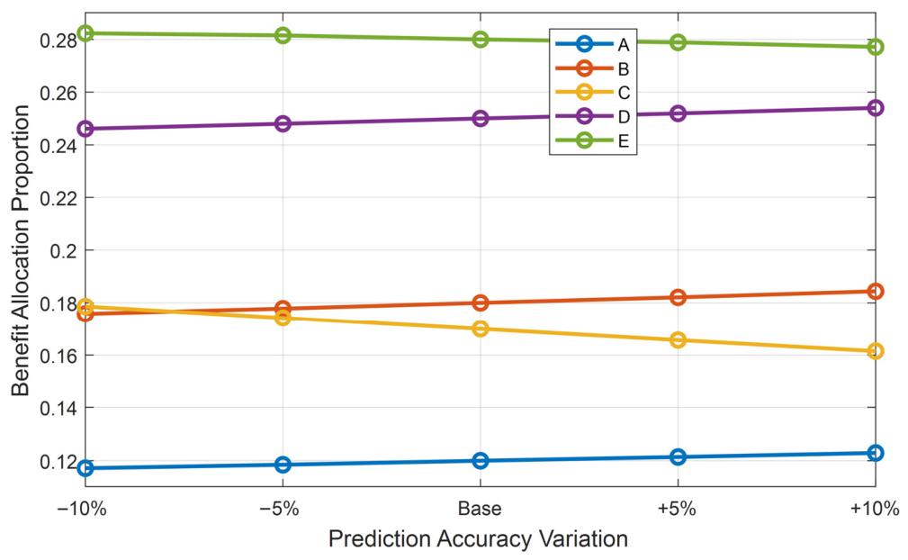
As shown in Figure 9, with the improvement in the prediction accuracy, the benefit allocation proportions of PV-only investors A and B increased steadily, while that of energy storage-only investor C decreased gradually. For hybrid investors D and E, their allocation shares rose slightly due to the enhanced contribution of PV units. The fluctuation of each investor’s proportion was limited within 10%, presenting a weak sensitivity. The variation trend conformed to the bargaining power mechanism of the Nash–Harsanyi game, which encourages members to improve the PV prediction performance and ensures stable and robust allocation results.
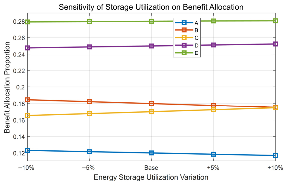
As shown in Figure 10, the increase in utilization significantly improved the benefit shares of storage-related investors. The allocation proportions of pure storage investor C and hybrid investors D and E rose steadily to compensate for the life loss and operation cost in frequency regulation, while those of non-storage investors A and B dropped slightly. The fluctuation was less than 6% with smooth variation. This rule strictly follows the principle of distribution according to contribution, motivating efficient operation of energy storage and maintaining the stability of the VPP alliance.

5. Conclusions

This paper focused on the multi-market trading strategy and benefit distribution of photovoltaic VPPs, constructed a three-stage stochastic optimization operation model and a payoff distribution mechanism based on game theory, and verified the effectiveness and practicality of the model through a case analysis. The main conclusions are as follows:
(1) The proposed three-stage stochastic optimization model improved the single-day market returns by 20.79%, 4.64% and 9.33%, respectively, compared with the independent operation, absolute FM and sequential optimization models. It also achieved an operating effect of distributed photovoltaic abandonment rate close to zero and a full-time FM performance score higher than 0.4.
(2) The return distribution model based on the Nash–Harsanyi bargaining game increased the returns of all investment entities, with an increase of between 3.36~99.43%. Among them, the returns of entities with a higher photovoltaic prediction accuracy improved the most significantly, effectively ensuring the long-term stability of the alliance.
(3) The combination of the photovoltaic and storage collaborative operation model guided by the VPP and the multi-market trading mechanism not only realized the efficient consumption of distributed photovoltaics and the optimal allocation of energy storage resources, but also improved the comprehensive profitability of VPPs through cross-market revenue collaboration, achieving a win–win situation of economic and social benefits. It provides a feasible paradigm for the operation of multi-agent cooperative VPPs, which combines economic benefits with engineering application value.

Author Contributions

Conceptualization, X.L.; methodology, G.M. and B.W.; formal analysis, N.C. and J.B.; investigation, Z.W. and X.Y.; writing—review and editing, C.Z. and Q.A. All authors have read and agreed to the published version of the manuscript.

Funding

Project supported by Major Special Science and Technology Project of Yunnan Province (202302AF080006).

Data Availability Statement

The data presented in this study are available on request from the corresponding author due to privacy/ethical restrictions.

Conflicts of Interest

Authors Xiang Li, Gaoquan Ma, Bangcan Wang, Na Cai, Junwei Bao, Zishi Wang, Xuan Yang were employed by the company Kunming Electric Power Trading Center Co., Ltd. The remaining authors declare that the research was conducted in the absence of any commercial or financial relationships that could be construed as a potential conflict of interest.

References

  1. Li, Z.; Li, W.; Zhang, Z.; Chang, G.; Lu, J.; Yue, G.; Li, L.; Ni, W. “Research on the development strategy of flexibility resources in my country’s power system under the dual carbon” goal. China Eng. Sci. 2024, 26, 108–120. [Google Scholar]
  2. Liu, D.; Bao, G.; Li, J.; Wang, J. Research on the configuration and pricing strategy of shared electricity-hydrogen hybrid energy storage capacity in integrated energy microgrid groups. Smart Power 2026, 54, 38–46. [Google Scholar] [CrossRef]
  3. Zhang, X.H.; Xu, C.B. Two-stage operation optimization of electric-hydrogen hybrid energy storage system with multi-type electrolysis coordination under wind-solar multi-frequency scale fluctuation. Acta Energiae Solaris Sin. 2026, 47, 702–713. [Google Scholar] [CrossRef]
  4. Liu, W.X.; Lv, X.Y.; Wan, H.Y.; Cheng, R. Research on multi-agent collaborative photovoltaic-energy storage operation strategy based on demand response. Mod. Electr. Power 2026, 43, 193–200. [Google Scholar] [CrossRef]
  5. Dai, J.; Xiang, Y.; Li, R.; Liu, J. Optimized configuration of photovoltaic storage aggregator capacity driven by virtual energy trading. Eng. Sci. Technol. 2023, 55, 152–159. [Google Scholar] [CrossRef]
  6. Li, J.M.; Jiang, J.M.; Yang, Q.N.; Ai, Q.; Wang, D.; Cai, N. Virtual power plant auxiliary service incentive mechanism and key technologies based on customized packages. Power Syst. Autom. 2025, 49, 34–50. [Google Scholar]
  7. Yang, C.; Xu, T.; Li, Y.; Li, X. Study on the scheduling strategy of energy storage aggregator auxiliary service market based on dynamic programming. J. Sol. Energy 2025, 46, 224–233. [Google Scholar] [CrossRef]
  8. Ni, F.; Guo, J.; Xiang, Y.; Liu, J. Multi-market hybrid game trading strategies for electric vehicle aggregators accounting for renewable energy consumption. China J. Electr. Eng. 2026, 1–13. [Google Scholar]
  9. Liu, J.; Liu, K.; Ke, X.; Tang, Z.; Deng, J. Energy storage in new power systems participates in the multi-market trading method of electric energy-inertia-primary frequency regulation. Grid Technol. 2025, 49, 1018–1031. [Google Scholar] [CrossRef]
  10. Sun, C.; Yin, W.; Zhang, Z.; Li, M.; Peng, K. Low-carbon economic coordinated scheduling method for cogeneration virtual power plants with multi-market participation. Power Eng. Technol. 2024, 43, 100–110. [Google Scholar]
  11. Yan, X.; Chen, Y.; Ma, J.; Huang, Z.; Zeng, Q.; Zeng, J. Comprehensive bidding strategies for electric vehicle aggregators participating in multiple markets that consider response uncertainty. Power Grid Technol. 2025, 49, 1459–1468. [Google Scholar] [CrossRef]
  12. Ahmed, M.U.; Qays, M.O.; Lachowicz, S.; Mahmud, P. Optimizing EV Battery Charging Using Fuzzy Logic in the Presence of Uncertainties and Unknown Parameters. Electronics 2026, 15, 177. [Google Scholar] [CrossRef]
  13. Duan, J.; Xie, J.; Zhao, X.; Chang, Y.; Ge, Y. Cooperative gain allocation strategy for wind-light-water-storage multi-agent complementary power generation system based on improved Shapley value method. Power Autom. Equip. 2024, 44, 22–30. [Google Scholar] [CrossRef]
  14. Zheng, C.; Jiang, Y. Wind power fluctuation cost sharing strategy based on improved Shapley value. Power Grid Technol. 2021, 45, 4387–4394. [Google Scholar] [CrossRef]
  15. Wei, Z.B.; Zhang, Z.Q.; Li, Y.J.; Li, J.; Yuan, K. Integrated model for microgrid planning and operation under multi-agent cooperation mode. Power Constr. 2024, 45, 47–58. [Google Scholar]
  16. Wu, D.; Yu, A. Profit distribution based on nucleolar theory in coordinated scheduling of large-scale multi-source joint export. Grid Technol. 2016, 40, 2975–2981. [Google Scholar] [CrossRef]
  17. Zhan, J.; Huang, M.; Sun, X.; Zhang, Y.; Chen, Z.; Chen, Y.; Li, Y.; Zhao, C.; Ai, Q. Optimization Strategy for Electricity–Carbon Sharing Operation of Multi-Virtual Power Plants Considering Multivariate Uncertainties. Energies 2025, 18, 2376. [Google Scholar] [CrossRef]
  18. Libra, M.; Mrázek, D.; Tyukhov, I.; Severová, L.; Poulek, V.; Mach, J.; Šubrt, T.; Beránek, V.; Svoboda, R.; Sedláček, J. Reduced real lifetime of PV panels—Economic consequences. Sol. Energy 2023, 259, 229–234. [Google Scholar] [CrossRef]
  19. Wang, Y.; Hao, L.; Xu, F.; Chen, W.; Zheng, L.; Chen, L.; Min, Y. Pattern Recognition and Ultra-Short-Term Probabilistic Forecasting of Power Fluctuating in Aggregated Distributed Photovoltaics Clusters. J. Shanghai Jiaotong Univ. 2024, 58, 1334–1343. [Google Scholar] [CrossRef]
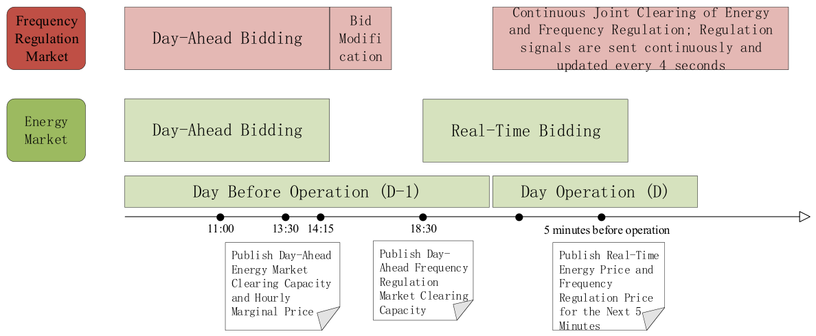
Figure 1. Multi-time-scale joint market operation architecture.
Electronics 15 02201 g001
Figure 2. Schematic diagram of a three-stage stochastic optimization model for a PV-storage VPP participating in multiple markets.
Electronics 15 02201 g002
Figure 3. (a) Day-ahead time-of-use forecast; (b) forecast curve on a daily basis.
Electronics 15 02201 g003
Figure 4. Results of optimization of the day-ahead bid for the first phase of the photovoltaic-storage VPP.
Electronics 15 02201 g004
Figure 5. (a) Results of the basis point optimization of the real-time operating power of the second-phase optical storage; (b) results of the third phase of real-time FM power optimization of optical storage; and (c) optimization results of actual operating power of optical storage.
Electronics 15 02201 g005
Figure 6. Distribution of target solar storage VPP FM performance scores.
Electronics 15 02201 g006
Figure 7. Income distribution plan for each investment entity participating in the photovoltaic-storage VPP.
Electronics 15 02201 g007
Figure 8. Comparison of market returns before and after each investment entity joined the alliance.
Electronics 15 02201 g008
Figure 9. Sensitivity analysis of prediction accuracy on benefit allocation.
Electronics 15 02201 g009
Figure 10. Sensitivity analysis of energy storage utilization on benefit allocation.
Electronics 15 02201 g010
Table 1. Classification of investment entities for three types of PV-storage VPPs.
Composition of Investment EntitiesType 1Type 2Type 3
Distributed photovoltaic-
Energy storage-
Table 2. Comparison of market returns of photovoltaic VPP under four models.
ModelBasic ModelModel IModel IIModel III
Earnings (yuan)15,605.2512,360.7314,881.1214,149.37
Percentage of earnings100%79.21%95.36%90.67%
Table 3. Percentage of daily and intraday forecast errors for each distributed photovoltaic individual.
Investment EntityTypePhotovoltaic Capacity (MW)Energy Storage Capacity (MW)Maximum Discharge Power (MW) of Energy StorageMaximum Charging Power (MW) of Energy StorageRisk Appetite Coefficient
AType I100.6
BType I300.6
CType II2010100.5
DType III3010550.7
EType III5010550.7
Total120402020
Table 4. Percentage of day-ahead and intra-day prediction errors of each distributed photovoltaic individual.
Investment EntityABDEWeighted
Average
Photovoltaic day-ahead prediction error15%20%20%25%22%
Intra-day prediction error of PV8%10%10%15%12%
Table 5. Results of the calculation of the utility function for each investment entity.
Investment EntitySerial NumberRisk Appetite CoefficientEnergy Storage Capacity (MW)
A10.6U1(φ1) = 5.2774 − 3.6774ln(4.2 − φ1)
B20.6U2(φ2) = 5.2774 − 3.6774ln(4.2 − φ2)
C30.5U3(φ3) = φ3
D40.7U4(φ4) = 1.4196 − 1.727ln(2.275 − φ4)
E50.7U5(φ5) = 1.4196 − 1.727ln(2.275 − φ5)
Table 6. Results of calculation of negotiation power and initial negotiation points of each investment entity.
Investment EntityBiMCBiFABiCPBiURαiφi,min
A0.12980.50000.20300.0501
B0.19050.26100.15980.1331
C0.05080.50000.50000.16840.1485
D0.34340.31700.25000.28210.23430.2225
E0.37120.13790.25000.38470.23450.3114
Disclaimer/Publisher’s Note: The statements, opinions and data contained in all publications are solely those of the individual author(s) and contributor(s) and not of MDPI and/or the editor(s). MDPI and/or the editor(s) disclaim responsibility for any injury to people or property resulting from any ideas, methods, instructions or products referred to in the content.