Improving Heart-Failure Predictive Tasks with Patient Health Knowledge Graphs and Sequential Graph Neural Networks

Abstract

Patient health knowledge graphs provide a means for high-quality and interoperable clinical data representation, while graph neural networks are a key enabler in order to learn their underlying relationships for downstream prediction tasks. In this work, we propose a sequential graph neural network (SeqGNN) framework that models patient visit trajectories for multiple binary clinical tasks, namely diagnosis, readmission, and mortality prediction. The proposed architecture integrates temporal dynamics with graph-based representations that enhances patient-level embeddings. Focusing on patients at the risk of Heart Failure (HF), our methodology achieves comparatively high accuracy and precision-versus-recall tradeoffs on highly heterogeneous graphs and imbalanced labeled data. We additionally quantify the uncertainty concerning each clinical decision making task and, compared with the state-of-the-art, show that AUROC and AUPRC scores reliably improve for onset diagnosis in particular, as high as 93.1 and 79.1 respectively. Our experiments conducted on real-world data from an intensive care unit demonstrate the potential for sequential representation learning over patient health knowledge graphs that can be provided for high-precision decision-making in clinical settings.

1. Introduction

The proliferation of electronic health records (EHRs) in recent years has resulted in an unprecedented accumulation of clinical data, encompassing patient interactions, events, and interrelated medical information. The growing availability of such datasets enables predictive modeling to support risk mitigation, optimize clinical workflows, and enhance patient care across multiple domains, including diagnosis [1,2], medication management [3], and procedural interventions [4,5]. Despite this potential, the deployment of predictive models in clinical settings remains constrained by the need for high precision and the complete integration of patient histories, among other challenges associated with heterogeneous, multi-source data [6].

Graph representation learning offers a compelling approach for capturing the complex relationships inherent in EHR data [7]. Graph neural networks (GNNs) can model both local and global dependencies among diverse clinical entities, including patient histories, diagnoses, medications, and procedures, through non-linear message-passing operations. These capabilities have been shown to improve predictive performance across tasks ranging from disease onset prediction to drug recommendation. Nonetheless, practical applications are often hampered by data heterogenity, fragmentation, and the sequential nature of patient histories, which, in turn, reduce representation quality [8], highlighting the need for unified frameworks that integrate temporal, multimodal, and graph-structured representations of patient data.

Existing approaches, a summary of which is provided in

Table 1. Summary of baseline models for clinical tasks-Dx: diagnosis, Rx: readmission, Mx: mortality.

Author	Year	Abbreviation	Methodology	Task
Choi et al. [9]	2016	RETAIN	Reverse Attention	Dx, Rx, Mx
Ma et al. [10]	2017	Dipole	Bidirectional Recurrent Neural Network	Dx
Luo et al. [11]	2020	HiTANet	Hierarchical Time-aware Attention Network	Dx
Ma et al. [12]	2020	AdaCare	Self-adaptive feature-extraction and recalibration	Rx, Mx
Gao et al. [13]	2020	StageNet	Long-short-term memory with stage progression	Rx, Mx
Zhange et al. [14]	2021	GRASP	Representation learning with patient similarities	Rx, Mx
Lu et al. [15]	2021	CGL	Collaborative graph learning with text and notes	Dx
Yang et al. [16]	2023	KGxDP	Path reasoning over knowledge graphs	Dx
Yang et al. [17]	2023	ManyDG	Variational autoencoder	Rx, Mx
Huang et al. [18]	2024	HEART	Heterogeneous relation-aware Transformer	Rx
Yang et al. [19]	2025	KCIF	Temporal Heterogeneous Graph Learning	Dx
Feng et al. [20]	2025	DemGraph	Context-driven Retrieval with Large Language Models	Rx
Li et al. [21]	2026	TCEM	Disease co-occurrence with temporal GNN	Dx

, remain particularly fragmented across tasks, input modalities, and time-dependent feature learning. Firstly, most existing approaches are task-specific with limited ability to learn generalizable representations. Secondly, many methods rely predominantly on codified data, with only a subset incorporating numerical features or clinical text, thus resulting in incomplete patient representations and under-utilization of available EHR modalities. Thirdly, while models capture temporal dependencies through sequential signals, they lack the ability to fully model complex interactions among diversified clinical events over time. Moreover, although recent works introduce graph-based components, they often use simplified or partially integrated graph structures without fully leveraging the structure-rich nature of patient health knowledge graphs for joint relational and temporal reasoning. Lastly, minimal attention has been paid to quantifying the uncertainty in model predictions, a key reliability requirement for practical clinical settings.

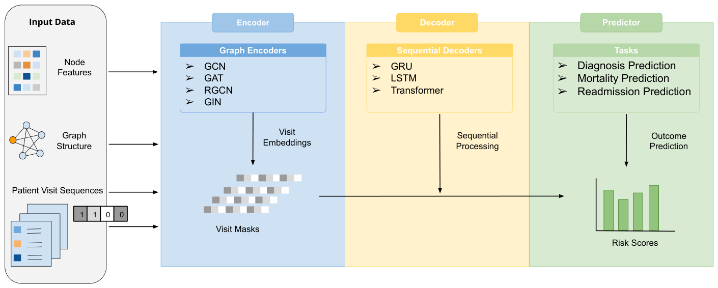
To address these limitations, in this work, we propose a modular framework that is end-to-end trainable for prediction across multiple tasks using a heterogeneous patient health knowledge graph (PHKG). We focus on patients at the onset of heart failure (HF) and apply our model for three individual tasks, namely HF diagnosis, mortality risk, and readmission rate prediction. These classification tasks are critical for downstream clinical processes; however, they are particularly difficult to predict due to high levels of comorbidity and weak correlations in data. The proposed approach, a Sequential Graph Neural Network (SeqGNN), captures the hidden structures from patient graphs and subsequently models temporal dependencies across visits for multiple downstream tasks via:

• A multi-type graph encoder generates contextualized embeddings in order to support the integration of numerical, textual, and codified information.
• A configurable sequential decoder, equipped with a learnable temporal component, in order to capture the longitudinal progression of clinical events across patient visits.
• A sequence-based predictor that supports (binary or multi-label) classification across different clinical tasks given fully integrated data as patient health knowledge graphs.
• Uncertainty quantification in order to provide insights into model performance related to HF predictive tasks through ensemble SeqGNN predictors.

Our approach is guided by three key research questions aimed at understanding both the behavior and design of SeqGNN models for clinical prediction tasks. Firstly, we analyze which components of sequential and longitudinal EHR modeling—such as temporal learning, multimodal data integration, and structural representations—most effectively inform model design for individual diagnosis, readmission, and mortality prediction tasks (RQ1). Secondly, we examine what uncertainty quantification and calibration analyses reveal about these models, with a focus on understanding their reliability, stability, and limitations across different clinical settings (RQ2). Thirdly, we investigate to what extent the relationship between prediction confidence and performance in ensemble SeqGNNs can inform model deployment, particularly in practical settings, identifying reliable predictions, limitations, and refinement strategies for future research (RQ3).

More specificaly, we construct a visit-centric PHKG from an electronic health record repository to model heart-failure-related outcomes. Hospital admissions are first filtered to retain only clinically confirmed HF cases using predefined ICD-9 codes. For each qualifying admission, four structured clinical domains are extracted: medications, abnormal laboratory measurements, procedures, and HF-specific diagnoses. Duplicates and incomplete entries are removed to ensure a consistent admission-level representation. Each admission is treated as a distinct visit node connected to its associated clinical concept nodes (medications, labs, procedures, diagnoses), forming heterogeneous, multi-relational subgraphs. Identical clinical concepts across admissions are represented by shared global nodes, enabling parameter sharing and cross-visit generalization when all admission-level subgraphs are merged into a single global PHKG.

To support sequential modeling, visits are grouped by patient identifier and ordered chronologically using admission timestamps, forming variable-length visit sequences per patient. Each visit retains its admission-level label (mortality, readmission, or multi-label HF phenotype). The graph structure models intra-visit clinical relationships, while the ordered visit sequences enable longitudinal learning across time. This design allows a sequential GNN framework to first encode each visit via message passing over the PHKG and subsequently model temporal dependencies across visits.

For node feature generation, concept nodes are enriched using both semantic and numerical representations. Textual descriptions of medications, laboratory findings, and procedures are encoded with a pre-trained sentence transformer, producing dense embeddings attached with concept nodes. For laboratory concepts, raw scalar values are additionally projected into vector space using a small feed-forward network and concatenated with text embeddings, preserving precise quantitative information. Visit nodes receive learnable embeddings and aggregate semantic signals implicitly through message passing rather than explicit feature pooling at construction time. This node-centric enrichment strategy yields a semantically expressive, numerically grounded heterogeneous PHKG suitable for sequential graph neural network modeling of heart failure prediction tasks.

Our evaluation considers three sequential prediction tasks derived from hospital admissions as binary classification problems: in-hospital mortality, readmission within a specified time frame, and heart failure diagnosis prediction. Tasks leverage chronological visit sequences processed by the graph encoder followed by the sequential decoder, enabling the model to integrate relational and temporal information effectively. We evaluate the model on the publically available MIMIC III dataset (accessed 13 March 2026 via: https://physionet.org/content/mimiciii/1.4/) including hospitalizations in an intensive care unit, in terms of the area under receiver operating (AUROC) and precision–versus–recall curves (AUPRC) as compared to the-state-of-the-art methods. In order to measure the applicability of the proposed method in real-world settings, we further conduct uncertainty quantification (UQ) experiments and show that with an increasing number of ensemble SeqGNNs, high-confidence predictions can be made in each task.

2. Patient Health Knowledge Graphs

Clinical information such as patient visits, diagnoses, medications, laboratory measurements, and procedures, are derived from hospital admissions. Each hospital admission is treated as a distinct clinical event and linked to a unique patient identifier, enabling the construction of longitudinal patient trajectories. The dataset is preprocessed to ensure consistency between admission records and encoded clinical entities, and subsequently transformed into a PHKG, where nodes represent clinical concepts and visits, and edges capture their relationships. This representation supports both relational modeling across heterogeneous medical entities and sequential modeling of chronologically ordered patient visits for downstream prediction tasks, as detailed in the following subsections.

2.1. Dataset

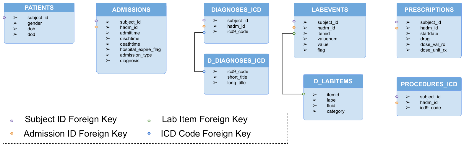
We use the MIMIC repository containing tabular data for patients to ultimately generate triples that form a PHKG for training and evaluation purposes. All records for a set of patients are extracted according to predefined criteria. The criteria by which the records are obtained include the intent for hospitalization, table names and concepts, as well as entity types and relations. The intent for hospitalization can be set in order to limit the scope of the task to a particular use case. In this work, records from patients that are hospitalized for heart failure (HF) are separated based on their ICD codes (i.e., International Classification of Diseases). Since many tables already exist as data sources for patients with a particular hospitalization intent, the scope is further narrowed down to main concepts related to any medication prescribed, lab results and measurements taken, hospital procedures performed, and diagnoses made. The relevant data are stored in separate tables and can be processed as such (please refer to Figure 1). Within each table, a subset of columns and relations is selected by examination as explained in subsequent sections. While the dataset is provided in two versions, in this study, the following versions is utilized:

MIMIC III—The first version of the repository that we use contains data associated with 53,423 distinct hospital admissions for adult patients (aged 16 years or above) admitted to critical care units between 2001 and 2012 covering 38,597 distinct adult patients overall. The median age of adult patients is 65.8 years, 55.9% patients are male, and in-hospital mortality is 11.5%. In addition, it contains data for 7870 neonates admitted between 2001 and 2008 (excluded from this study). The median length of an ICU stay is 2.1 days and the median length of a hospital stay is 6.9 days. A mean of 4579 charted observations (‘chartevents’) and 380 laboratory measurements (‘labevents’) are available for each hospital admission.

Figure 1. MIMIC III tables used in this study and connections through a foreign key.

Figure 1. MIMIC III tables used in this study and connections through a foreign key.

We utilize admission-level information from the admission table, which provides patient identifiers, admission and discharge timestamps, in-hospital mortality indicators, and primary diagnosis descriptions. Clinical events associated with each hospital admission are retrieved from four primary tables: ICD-9 diagnosis codes, ICD-9 procedure codes, medication orders including drug names, National Drug Codes (NDC), and dosage information, and laboratory measurements. For each admission, structured codes are extracted and filtered to remove missing or duplicate entries (medications without NDC codes and laboratory records without measurements). The resulting admission-level representation includes diagnosis codes, procedure codes, medication identifiers, and laboratory-item identifiers, together with numerical laboratory values stored as literals. This preprocessing step yields a consistent, admission-centric dataset that supports both relational graph construction and longitudinal patient-level modeling.

More precisely and as shown in Figure 1, the PATIENTS table provides demographic information (e.g., age, gender, date of death) linked via subject_id, while ADMISSIONS defines hospital visits using hadm_id and includes key outcome variables such as hospital_expire_flag, admission and discharge timestamps, and admission type. Diagnostic and procedural information is recorded in DIAGNOSES_ICD and PROCEDURES_ICD, respectively, using ICD-9 codes associated with each admission. Medication administrations are extracted from PRESCRIPTIONS, which provides drug names and dosage details. The D_ICD_DIAGNOSES table serves as the reference dictionary for ICD-9 diagnosis codes in MIMIC-III. Laboratory measurements are obtained from LABEVENTS, including numeric results, abnormality flags, and timestamps, with metadata definitions available in D_LABITEMS. Together, subject_id and hadm_id form the relational backbone of the database, enabling the construction of admission-centric heterogeneous graphs for mortality prediction, readmission modeling, and heart failure outcome analysis.

Heart failure admissions were identified by scanning diagnosis records for the presence of any of the ICD-9 codes listed in

Table 2. ICD-9 diagnosis codes used to identify heart failure admissions.

ICD-9 Code	Clinical Phenotype
428.00	Congestive heart failure, unspecified
428.10	Left heart failure
428.20	Systolic heart failure, unspecified
428.21	Acute systolic heart failure
428.22	Chronic systolic heart failure
428.23	Acute on chronic systolic heart failure
428.30	Diastolic heart failure, unspecified
428.31	Acute diastolic heart failure
428.32	Chronic diastolic heart failure
428.33	Acute on chronic diastolic heart failure
428.40	Combined systolic and diastolic heart failure, unspecified
428.41	Acute combined systolic and diastolic heart failure
428.42	Chronic combined systolic and diastolic heart failure
428.43	Acute on chronic combined systolic and diastolic heart failure
428.90	Heart failure, unspecified

. These codes collectively capture the full range of heart failure phenotypes, including acute, chronic, systolic, diastolic, and unspecified forms. Every hospital admission containing at least one of these codes was retained for graph construction, ensuring that only clinically confirmed heart failure episodes entered the final dataset. In total, 10,154 unique patients were included with one or more heart-failure diagnosis. We included all visits related to a patient with heart-failure diagnosis for a total 13,608 admissions. These admissions include 1192 unique procedure codes, 15 unique diagnosis codes, 265 unique lab item codes, and 3498 unique medication codes. Further statistics related to the dataset utilized in this study are shown in

Table 3. Dataset statistics for patients with heart failure diagnosis from MIMIC III repository.

Description	Symbol	Occurrences
HF Patients	$\left|P\right|$	10,154
HF Admissions	$|V_P|$	13,608
Unique diagnosis codes	$|{\mathcal{D}}_p|$	15
Unique observable codes	$|{\mathcal{O}}_p|$	265
Unique medication codes	$|{\mathcal{M}}_p|$	3498
Unique procedural codes	$|{\mathcal{R}}_p|$	1192
Average diagnosis per visit	$|{\mathcal{D}}_p\cap v_p^t|$	1.52
Average observable per visit	$|{\mathcal{O}}_p\cap v_p^t|$	196
Average medication per visit	$|{\mathcal{M}}_p\cap v_p^t|$	43.9
Average procedure per visit	$|{\mathcal{R}}_p\cap v_p^t|$	4.84

.

2.2. Classification Tasks

Labels for downstream prediction tasks are derived directly from structured fields within the MIMIC-III database at the hospital admission level. All tasks are formulated at the visit level and subsequently organized into chronological patient sequences for sequential modeling. For all tasks, admission-level labels are grouped by patient identifier and ordered chronologically using admission timestamps. This results in variable-length visit sequences per patient. During model training, sequences are padded to a uniform length and accompanied by masking vectors to ensure that loss computation and evaluation metrics are applied only to valid visits. The classification sequences and labels for each task are extracted as follows:

Heart Failure Diagnosis—Heart failure diagnosis labels are derived from the DIAGNOSES_ICD table. For each hospital admission, all ICD-9 diagnosis codes are examined, and the presence of any HF-specific codes listed in Table 2 is recorded. Unlike mortality and readmission, HF diagnosis prediction is formulated as a multi-label classification task: each admission may contain multiple HF-related ICD-9 codes simultaneously. A binary indicator vector is constructed per admission, where each dimension corresponds to one HF ICD-9 code, taking value 1 if the code is present and 0 otherwise. This produces a structured multi-label representation aligned with the admission-level graph nodes. For each index admission, subsequent admissions within a 365-day window are examined to determine whether a heart-failure diagnosis code appears. If a predefined heart-failure code is observed during a future admission within the specified window, the index admission is labeled as positive. Patients with fewer than two admissions are excluded because the occurrence of future heart failure cannot be determined. Using the full MIMIC-III dataset, 20,676 heart HF diagnosis records corresponding to 13,608 unique admissions were found. Importantly, during experiments for this task, the labeled data are excluded from the original PHKG using the test set.

In-Hospital Mortality—In-hospital mortality labels are obtained from the admission table using the hospital_expire_flag field. This binary indicator takes value 1 if the patient died during the hospital stay and 0 otherwise. Each hospital admission is therefore assigned a single binary mortality label. For sequential modeling, mortality labels are aligned with their corresponding admission timestamps and ordered chronologically per patient. Because the outcome occurs within the same hospital stay, label construction does not require information from subsequent admissions. Consequently, patients with a single recorded admission can be included in this task.

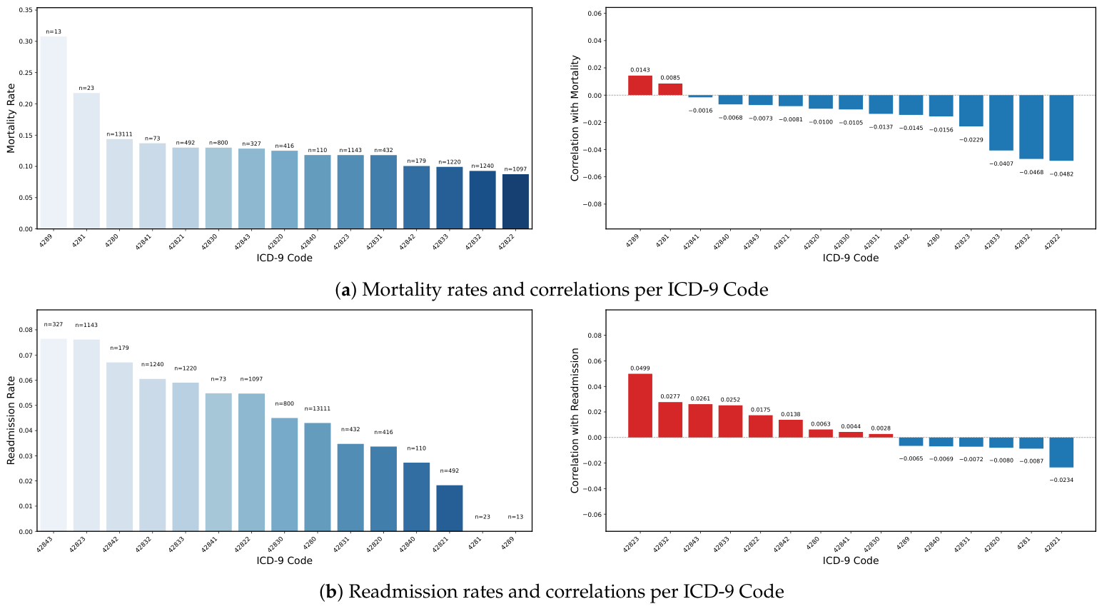
As shown in Figure 2, mortality rates varied across codes, with the highest rates observed for 4289 (30.8%) and 4281 (21.7%), although these codes occurred in relatively small numbers of admissions (13 and 23, respectively). The most prevalent code, 4280 (congestive heart failure unspecified), appeared in 13,111 admissions and had a mortality rate of 14.4%, reflecting its broad use in clinical coding. Most other HF subtypes showed mortality rates between 8.8% and 13.7%, indicating moderate variation across HF diagnoses. Correlation analysis between the presence of individual HF codes and mortality revealed very weak associations overall, with small positive correlations for 4289 ($r\approx 0.014$) and 4281 ($r\approx 0.008$), while most codes showed slightly negative correlations, such as 42,822 ($r\approx -0.048$) and 42,832 ($r\approx -0.047$). These results suggest that individual HF ICD-9 codes alone have limited predictive value for in-hospital mortality, although rare or unspecified HF codes appear to be associated with somewhat higher observed mortality rates.

Hospital Readmission—Hospital readmission is defined as a binary outcome indicating whether a patient is readmitted within a predefined temporal window following discharge (e.g., 30 days). For each admission, the discharge timestamp (dischtime) is compared to the admission time (admittime) of the next hospitalization for the same patient. If the time difference falls within the specified threshold, the current admission is labeled as a positive readmission case. The final admission of each patient sequence is excluded from readmission labeling, as no subsequent visit exists for comparison. This procedure yields one binary readmission label per admission. Labels are generated by examining the time difference between consecutive admissions for the same patient. Admissions resulting in in-hospital death are excluded from this task because readmission cannot occur in such cases. Since the label depends on the presence of a subsequent admission, only patients with at least two admissions are retained.

Overall, as shown in Figure 2, readmission rates were relatively low (generally between 2% and 8%), with the highest rates observed for ICD-9 code 42,843 (7.65%) and 42,823 (7.61%), followed by 42,842 (6.70%) and 42,832 (6.05%). These findings suggest that certain HF subtypes are associated with slightly higher short-term readmission risk. The most common code, 4280 (congestive heart failure unspecified), appeared in 13,111 admissions and had a readmission rate of 4.30%, reflecting its broad clinical use. Correlation analysis between the presence of individual HF codes and 30-day readmission showed generally weak associations, with the strongest positive correlations observed for 42,823 ($r\approx 0.05$), 42,832 ($r\approx 0.028$), and 42,843 ($r\approx 0.026$). Several codes showed near-zero or slightly negative correlations (e.g., 42,821, $r\approx -0.023$). Overall, these results suggest that HF ICD-9 codes alone provide limited predictive power for short-term readmission, although certain acute or more specific HF subtypes exhibit slightly stronger associations with readmission risk.

2.3. Patient Health Knowledge Graph Construction

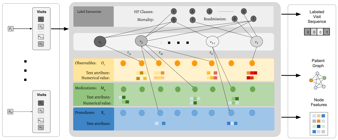
To enable graph neural network modeling of heart failure outcomes, we construct a collection of visit-centric heterogeneous Patient Health Knowledge Graphs (PHKGs) derived exclusively from heart-failure hospitalizations explained above. The objective is to represent each admission as a structured, multi-relational graph that preserves both clinical semantics and relational topology. Let P denote the cohort of patients. For each patient $p\in P$, define ${\mathcal{O}}_p$, ${\mathcal{D}}_p$, ${\mathcal{M}}_p$, and ${\mathcal{R}}_p$ as the sets of laboratory observations, diagnoses, medications, and procedures, respectively. The complete set of encoded clinical concepts is given by: ${\mathcal{C}}_p={\mathcal{O}}_p\cup {\mathcal{D}}_p\cup {\mathcal{M}}_p\cup {\mathcal{R}}_p$. Visits are chronologically ordered as $\{v_p^1,\dots ,v_p^T\}$, where each visit satisfies $v_p^t\subseteq {\mathcal{C}}_p$. Without loss of generality, we let T be the maximum number of visits and pad shorter sequences accordingly.

The PHKG is defined as a heterogeneous graph $G=(V,E,R)$ with a node set consisting of ${\bigcup }_{p\in P}\left\{v_p^t\right\}$ union ${\bigcup }_{p\in P}{\mathcal{C}}_p$. Edges connect visit nodes to clinical concept nodes according to relation type $r\in R=\{r_M,r_O,r_R,r_D\}$, corresponding to medication, abnormal laboratory observation, procedure, and heart-failure-specific diagnosis, respectively. Formally, the edge set over the patient visits is given as follows: $E=\{(v_p^t,r,c)\mid c\in v_p^t,r\in R\}$. Each node $u\in V$ is initialized with a learnable embedding vector ${\mathbf{x}}_u$$\in {\mathbb{R}}^d$. For laboratory concepts $c\in {\mathcal{O}}_p$ with numeric measurements, the scalar value is incorporated as a literal attribute of the corresponding node. A categorical node-type indicator distinguishes visit nodes from concept nodes, enabling heterogeneous encoding.

Visit-specific subgraphs are retained only if $|{\mathcal{M}}_p\cap v_p^t| \ge 1$, $|{\mathcal{O}}_p\cap v_p^t| \ge 1$, and $|{\mathcal{R}}_p\cap v_p^t| \ge 1$, ensuring that each admission graph contains sufficient multimodal information. All admission-level subgraphs are subsequently merged into a single global graph PHKG, where identical clinical concepts across visits are represented by shared nodes. This global integration enables parameter sharing and the learning of generalized representations across hospitalizations. By jointly encoding typed predicate relations, numerical laboratory attributes, and semantic embeddings, the PHKG provides a comprehensive and expressive representation for downstream graph neural network tasks.

2.4. Feature Enrichment

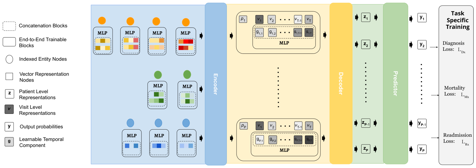
To provide rich and semantically meaningful node representations, we enrich both visit nodes and clinical concept nodes with two complementary types of features: high-dimensional semantic embeddings derived from textual descriptions and learned vector representations of numerical measurements.

Textual Attributes—All clinical concepts in medications (${\mathcal{M}}_p$), laboratory observations (${\mathcal{O}}_p$), and procedures (${\mathcal{R}}_p$) with labels (concise natural-language descriptions) are further processed to improve feature representations as follows. Medication descriptions combine drug name, dose, route, and unit (e.g., “aspirin 81 mg oral tablet”). Laboratory observations incorporate the measured value, unit, and reference context (e.g., “potassium 3.2 mEq/L low”). Procedure descriptions use the standardized long-title text from the procedure coding system (e.g., “Coronary artery bypass graft”). Each textual description is encoded using a pre-trained sentence transformer, yielding a fixed d-dimensional embedding vector ${\mathbf{e}}_c\in {\mathbb{R}}^d$ for every concept c. These embeddings are attached directly to the corresponding concept nodes in the graph. For each visit $v_p^t$, the semantic information is implicitly propagated from its associated concept nodes during message passing, eliminating the need for explicit visit-level aggregation at construction time.

Numerical Attributes—Numerical laboratory measurements (scalar values associated with concepts in ${\mathcal{O}}_p$) are handled in two steps. First, the raw scalar is converted into a textual description (e.g., “potassium 3.2 mEq/L”) and embedded as described above, ensuring the numerical information contributes to the node’s semantic representation. Second, to preserve precise quantitative signal, the raw scalar value is projected into a d-dimensional vector using a small shared multi-layer perceptron (MLP):

$$\begin{array}{c}\hfill {\mathbf{q}}_c=\mathrm{MLP}\left(\mathrm{scalar}\left(c\right)\right)\in {\mathbb{R}}^d,\end{array}$$

(1)

where the MLP consists of two linear layers with Rectified Linear Unit (ReLU) activation. The projected vector ${\mathbf{q}}_c$ is concatenated with the text-derived embedding ${\mathbf{e}}_c$ and attached directly to the laboratory concept node c. This fused representation enables the graph encoder to jointly reason over linguistic clinical context and exact numerical measurements during message passing.

By attaching both text-derived semantic embeddings and MLP-projected numerical vectors directly to the concept nodes, the PHKG nodes become richly annotated with clinically meaningful features. This node-centric enrichment strategy leverages the graph structure to propagate and integrate information across visits and concepts, providing a powerful and homogeneous input to downstream graph neural network tasks, as shown in Figure 3.

3. Methodology

This section presents the proposed sequential heterogeneous graph neural network (termed SeqGNN) for modeling patient trajectories using the PHKG generation process described above for binary classification tasks: (i) in-hospital mortality, (ii) 30-day readmission, and (iii) heart-failure diagnosis. All tasks operate on identical visit-centric representations while respecting the exact chronological order of admissions, thereby capturing both intra-admission relational semantics and inter-admission temporal dynamics. The overall framework consists of two complementary stages, as shown in Figure 4. First, a graph encoder aggregates multi-type relational information from the PHKG to produce visit-level embeddings. Second, a sequential decoder processes the ordered visit embeddings after explicit augmentation with temporal spacing features, generating admission-level predictions. This design ensures that variable time intervals between hospitalizations—clinically meaningful indicators of disease progression or stability—are directly encoded rather than inferred solely from sequence position.

3.1. Heterogeneous Encoder

The graph encoder $\mathrm{Encoder}(·)$ operates exclusively on visit subgraphs to capture intra-visit relationships between medical concepts. Let V comprise all visit nodes $v_p^t$ and concept nodes. Each node $u\in V$ receives an initial feature vector ${\mathbf{x}}_u\in {\mathbb{R}}^d$ formed by a learnable identity embedding, textual semantic embeddings ${\mathbf{e}}_c$ (from a sentence transformer) for all concept nodes, and—for laboratory nodes—an additional numerical projection ${\mathbf{q}}_c$ (two-layer MLP with ReLU) of the raw scalar measurement as before. These features for patient p assemble into the matrix ${\mathbf{X}}_p$ with which the encoder then computes visit representations as follows:

$$\begin{array}{c}\hfill {\mathbf{H}}_p=\mathrm{Encoder}({\mathbf{X}}_p,G),\end{array}$$

(2)

where $G=(V,E,R)$ as the patient health knowledge graph as before and ${\mathbf{H}}_p=[{\mathbf{h}}_{v_p^1},\dots ,{\mathbf{h}}_{v_p^T}]$, padded to length T with masking vectors. Visit embeddings ${\mathbf{h}}_{v_p^t}\in {\mathbb{R}}^d$ are extracted from ${\mathbf{H}}_p$ for feature enrichment, each representing the patient’s clinical state during admission t.

To capture irregular time intervals between hospital admissions—a clinically critical signal reflecting disease progression, recovery, or acute decompensation—the model incorporates time-delta features. Let $\Delta t_{p,t}$ denote the number of days between visits $t-1$ and t (extracted from admittime timestamps in the MIMIC-III ADMISSIONS table). By convention, $\Delta t_{p,1}=0$ for the first admission of each patient. The normalized temporal feature is given as follows:

$$\begin{array}{c}\hfill {\widetilde{\Delta t}}_{p,t}=log(\Delta t_{p,t}+1).\end{array}$$

(3)

The logarithmic transformation compresses the extremely wide dynamic range of real-world inter-admission intervals (from same-day transfers to multi-year gaps) into a numerically stable scalar, preventing large values from dominating gradients while preserving relative ordering. This scalar is expanded into a low-dimensional embedding and concatenated with the visit representation:

$$\begin{array}{c}\hfill {\tilde{\mathbf{h}}}_{p,t}=[{\mathbf{h}}_{v_p^t}\parallel \mathbf{g}\left({\widetilde{\Delta t}}_{p,t}\right)],\end{array}$$

(4)

where $\mathbf{g}(·)$ is a learnable two-layer MLP with ReLU activation that projects the normalized interval into the same space as the visit embedding. Concatenation explicitly injects absolute timing information into every decoder step, enabling the model to learn that short $\Delta t$ values often correlate with elevated readmission or mortality risk, while long intervals indicate stabilization. This augmentation is applied uniformly before any sequential processing, guaranteeing compatibility with both recurrent and attention-based decoders.

Four representative architectures are utilized for the encoder stage, each producing d-dimensional visit embeddings strictly on the visit subgraphs. A summary of these modules are shown in

Table 4. Summary of encoder and decoder architectures evaluated in this study. Encoders learn topology-aware node representations, whereas decoders map learned embeddings to task-specific outputs.

Component	Architectural Characteristics	Methodological Advantages
Encoders
GCN [22]	Spectral graph convolution with normalized adjacency-based message passing; stacked layer propagation	Computationally efficient; stable optimization; strong performance on homophilic graph structures
GAT [23]	Multi-head self-attention applied to graph neighborhoods; adaptive attention coefficients	Learns importance weights for neighboring nodes; improved expressive capacity over static aggregation schemes
GIN [24]	MLP-based aggregation with trainable scaling parameter; deep feature transformation	High theoretical expressive power; strong ability to distinguish complex graph structures
RGCN [25]	Relation-specific transformation matrices; multi-relational message passing	Explicit modeling of heterogeneous edge types; well-suited for knowledge graphs and predicate-aware learning
Decoders
LSTM [26]	Recurrent neural network with gated memory cells designed for sequential data modeling	Captures long-range temporal dependencies in patient visit sequences; effective for modeling longitudinal clinical trajectories
GRU [27]	Gated recurrent unit architecture with simplified gating mechanism relative to LSTM	Computationally efficient sequential modeling; fewer parameters while retaining strong temporal representation capacity
Transformer [28]	Multi-head self-attention layers with feedforward sub-blocks	Captures global feature dependencies; adaptive feature weighting; high representational flexibility

. The layer-wise update rules follow standard conventions and each variant is chosen to span distinct aggregation paradigms, allowing for systematic quantification of how different message-passing mechanisms interact with the heterogeneous clinical topology.

Graph Convolutional Network (GCN)—this operator performs symmetric normalized aggregation for visit nodes using the neighbourhood of its given medical concepts through:

$$\begin{array}{c}\hfill {\mathbf{h}}_v^{(l+1)}=\sigma \left({\tilde{\mathbf{D}}}^{-1/2}\tilde{\mathbf{A}}{\tilde{\mathbf{D}}}^{-1/2}{\mathbf{H}}^{\left(l\right)}{\mathbf{W}}^{\left(l\right)}\right),\end{array}$$

(5)

where $\tilde{\mathbf{A}}=\mathbf{A}+\mathbf{I}$ adds self-loops to adjacency matrix $\mathbf{A}$ and $\tilde{\mathbf{D}}$ is the corresponding degree matrix; superscript l denotes layer index; and $\sigma$ is a non-linear activation function. This formulation implements a localized first-order approximation of spectral convolution. Degree-normalized aggregation stabilizes training on graphs with highly variable node degrees (common in clinical settings where frequently prescribed medications connect to many visits), while self-loops preserve a node’s own identity and mitigate over-smoothing across layers.

Graph Attention Network (GAT)—this module employs multi-head self-attention to incorporate short- and long-term influences while updating nodes. For each attention head k, the output representations at layer l is given by:

$$\begin{array}{c}\hfill {\mathbf{h}}_v^{(l+1)}=\parallel \sigma \left(\sum _{u\in \mathcal{N}\left(v\right)}{\alpha }_{vu}^k{\mathbf{W}}^k{\mathbf{h}}_u^{\left(l\right)}\right),\end{array}$$

(6)

where $\mathbf{W}$ are learnable parameters, and $\mathcal{N}$ is the set of neighbors, with attention coefficients computed as follows:

$$\begin{array}{c}\hfill {\alpha }_{vu}^k={\displaystyle \frac{exp\left(\mathrm{LeakyReLU}\left({\mathbf{a}}^{k\top }[{\mathbf{W}}^k{\mathbf{h}}_v^{\left(l\right)}\parallel {\mathbf{W}}^k{\mathbf{h}}_u^{\left(l\right)}]\right)\right)}{{\sum }_{w\in \mathcal{N}\left(v\right)}exp\left(\mathrm{LeakyReLU}\left({\mathbf{a}}^{k\top }[{\mathbf{W}}^k{\mathbf{h}}_v^{\left(l\right)}\parallel {\mathbf{W}}^k{\mathbf{h}}_w^{\left(l\right)}]\right)\right)}}.\end{array}$$

(7)

The learned attention weights ${\alpha }_{vu}^k$ dynamically assign importance to neighbors (e.g., an abnormal laboratory result receives a higher weight than a routine procedure), while multiple heads capture diverse relational perspectives. The concatenation operation ∥ preserves expressive capacity without forcing early averaging of attention heads.

Relational Graph Convolutional Network (RGCN)—in order to support multiple relation types R common in clinical patient graph, the RGCN applies relation-specific transformations given by:

$$\begin{array}{c}\hfill {\mathbf{h}}_v^{(l+1)}=\sigma \left(\sum _{r\in \{r_M,r_O,r_R\}}\sum _{u\in {\mathcal{N}}_r\left(v\right)}{\displaystyle \frac{1}{c_{v,r}}}{\mathbf{W}}_r^{\left(l\right)}{\mathbf{h}}_u^{\left(l\right)}+{\mathbf{W}}_0^{\left(l\right)}{\mathbf{h}}_v^{\left(l\right)}\right),\end{array}$$

(8)

where $c_{v,r}$ normalizes by neighborhood size under relation r and ${\mathbf{W}}_r^{\left(l\right)}$ represents relation-specific weight matrices. This design explicitly differentiates information flow from medications, laboratories, and procedures—crucial in a heterogeneous knowledge graph—while the self-loop term ${\mathbf{W}}_0$ retains node identity.

Graph Isomorphism Network (GIN)—this module enhances the representation learning using visit nodes through updates given by:

$$\begin{array}{c}\hfill {\mathbf{h}}_v^{(l+1)}={\mathrm{MLP}}^{\left(l\right)}\left((1+{ϵ}^{\left(l\right)}){\mathbf{h}}_v^{\left(l\right)}+\sum _{u\in \mathcal{N}\left(v\right)}{\mathbf{h}}_u^{\left(l\right)}\right),\end{array}$$

(9)

followed by batch normalization and a multi-layer perceptron. The injective aggregation $(1+ϵ){\mathbf{h}}_v+\sum {\mathbf{h}}_u$ combined with an MLP makes GIN provably equivariant with respect to symmetric properties, enabling it to distinguish subtle structural differences among clinical admission patterns.

3.2. Sequential Decoder

The augmented visit embeddings are processed by a sequential decoder $\mathrm{Decoder}(·)$ that models longitudinal dependencies and produces prediction logits for each admission. Given enriched and sequential visit features ${\tilde{\mathbf{H}}}_p=[{\tilde{\mathbf{h}}}_{v_p^1},\dots ,{\tilde{\mathbf{h}}}_{v_p^T}]$ for patient p, the decoder computes the patient-level representations (i.e., readouts) as follows:

$$\begin{array}{c}\hfill {\mathbf{Z}}_p=\mathrm{Decoder}\left({\tilde{\mathbf{H}}}_p\right),\end{array}$$

(10)

where admission logits ${\mathbf{z}}_{p,t}\in {\mathbb{R}}^d$ are updated using a sequential decoder of choice. We employ three different architectures as follows, a summary of which is shown in Table 4.

Recurrent Decoders—in order to capture the progression of patient visits, at time step t, the hidden state corresponding to visit-specific representations with feature enhancement is updated as follows:

$$\begin{array}{c}\hfill {\mathbf{s}}_t=\mathrm{RNN}({\tilde{\mathbf{h}}}_{p,t},{\mathbf{s}}_{t-1}),\end{array}$$

(11)

where ${\mathbf{s}}_t$ represents the patient’s latent clinical state after the t-th admission. The hidden state is projected to prediction logits via:

$$\begin{array}{c}\hfill {\mathbf{z}}_{p,t}={\mathbf{W}}_o{\mathbf{s}}_t+{\mathbf{b}}_o.\end{array}$$

(12)

Here, ${\mathbf{W}}_o$ is a set of learnable weights and ${\mathbf{b}}_o$ is the bias term. Long-Short Term Memory (LSTM) maintains a dedicated cell state to retain long-range temporal context across irregular admission gaps, while Gated Recurrent Unit (GRU) offers parameter-efficient gating suitable for shorter patient trajectories; both architectures now directly condition gating on the explicit time-delta embedding, allowing the model to modulate memory retention based on elapsed time since the prior visit.

Transformer Decoder—as an alternative, a Transformer can be considered to model the patient trajectories present across PHKG. After adding positional encodings, the input sequence to the Transformer is defined as ${\mathbf{Z}}^{\left(0\right)}=[{\tilde{\mathbf{h}}}_{p,1}+{\mathbf{p}}_1,\dots ,{\tilde{\mathbf{h}}}_{p,T}+{\mathbf{p}}_T]$, where ${\mathbf{p}}_t$ denotes learnable positional encodings. Stacked self-attention layers then compute as follows:

$$\begin{array}{c}\hfill {\mathbf{Z}}^{\left(l\right)}=\mathrm{MultiHeadAttn}\left({\mathbf{Z}}^{(l-1)}\right)+{\mathbf{Z}}^{(l-1)},\end{array}$$

(13)

with a multi-head attention network at layer l, followed by feed-forward transformations:

$$\begin{array}{c}\hfill {\mathbf{Z}}^{\left(l\right)}=\mathrm{FFN}\left({\mathbf{Z}}^{\left(l\right)}\right)+{\mathbf{Z}}^{\left(l\right)}.\end{array}$$

(14)

Self-attention allows each visit to attend to all previous admissions. The explicit time-delta embeddings supplement the learned positional encodings, supplying absolute interval magnitudes that pure ordinal position cannot convey and enabling the Transformer to discover clinically meaningful temporal patterns (e.g., rapid readmissions) across arbitrary sequence lengths. In Figure 5, the components of the model, including trainable textual and temporal MLP modules along with input and output representations, are viewed.

3.3. Task-Specific Prediction

Combining the encoder and decoder, the prediction for each visit is computed as follows:

$$\begin{array}{c}\hfill {\widehat{y}}_{p,t}=\sigma \left(f_{\theta }\left({\left\{{\mathbf{h}}_{p,t}\right\}}_{t=1}^T\right)\right),\end{array}$$

(15)

where $\sigma (·)$ is the sigmoid function and $f_{\theta }\left(\right)$ is the end-to-end trainable model with parameter set $\theta$ taken over both the encoder and decoder of choice. This formulation ensures that every prediction is conditioned on the full history of enriched visit embeddings up to time t, with both textual semantic context and explicit temporal spacing fully integrated. All encoder–decoder combinations are trained end-to-end. Model parameters $\theta$ (including all GNN weights ${\mathbf{W}}^{\left(l\right)}$, decoder weights, embedding matrices, time-projection MLP $\mathbf{g}$, and output projection ${\mathbf{W}}_o$) are updated via stochastic gradient descent on the task-specific losses defined below. Gradients are computed through the full computational graph—from node feature initialization, through graph message passing, temporal augmentation, sequence processing, and final sigmoid activation—using automatic differentiation.

This unified optimization allows the graph encoder, temporal feature projector, and sequential decoder to co-adapt, jointly learning clinically meaningful representations from raw EHR data. For each task, we optimize the model parameters independently using the following objective functions. The in-hospital mortality task is formulated as binary classification at the visit level. The loss is the average binary cross-entropy over all training visits $N=|V_{\mathrm{train}}|$:

$$\begin{array}{c}\hfill {\mathcal{L}}_{\mathrm{Mx}}=-{\displaystyle \frac{1}{N}}\sum _{p,t}\left[y_{p,t}log{\widehat{y}}_{p,t}+(1-y_{p,t})log(1-{\widehat{y}}_{p,t})\right],\end{array}$$

(16)

where $y_{p,t}\in \{0,1\}$ is the ground-truth mortality indicator and ${\widehat{y}}_{p,t}=\sigma \left(z_{p,t}\right)$ is the model-predicted probability. The readmission task uses an identical binary cross-entropy formulation:

$$\begin{array}{c}\hfill {\mathcal{L}}_{\mathrm{Rx}}=-{\displaystyle \frac{1}{N}}\sum _{p,t}\left[y_{p,t}log{\widehat{y}}_{p,t}+(1-y_{p,t})log(1-{\widehat{y}}_{p,t})\right].\end{array}$$

(17)

The final admission of each patient is excluded from this loss because no subsequent visit exists for comparison. Lastly, heart-failure diagnosis is treated as a binary classification problem (having one of the HF ICD-9 codes) with a loss that averages over both visits and labels:

$$\begin{array}{c}\hfill {\mathcal{L}}_{\mathrm{Dx}}=-{\displaystyle \frac{1}{NC}}\sum _{p,t}{\displaystyle \sum _{c=1}^C}\left[y_{p,t,c}log{\widehat{y}}_{p,t,c}+(1-y_{p,t,c})log(1-{\widehat{y}}_{p,t,c})\right].\end{array}$$

(18)

where C is the number of heart-failure diagnosis codes. This formulation ensures balanced supervision across rare and common codes while enabling multi-task learning when combined with the other objectives. The overall optimization framework is shown in Algorithm 1. In the next section, we carry out experiments in order to demonstrate how graph aggregation and sequential modeling jointly improve performance. We use standard AUROC and AUPRC metrics to evaluate mortality and readmission prediction at patient level as a binary classification task. For diagnosis prediction, multiple diagnosis codes are aggregated into a single binary label indicating the presence or absence of HF, for which a binary F1-score is reported.

Algorithm 1 Sequential Graph Neural Network

Require:  PHKG $G=(V,E,R)$, patient set $\mathcal{P}$, maximum sequence length T, time-deltas $\{\Delta t_p^t\}$ Ensure:  Visit-level predictions $\left\{{\widehat{y}}_{p,t}\right\}$     # Step 1: Initialize node features 1: for each node $u\in V$ do 2:     ${\mathbf{x}}_u\leftarrow$ learnable embedding of u 3:     if u is a concept node then 4:         ${\mathbf{x}}_u\leftarrow [{\mathbf{x}}_u\parallel {\mathbf{e}}_u]$                                                                        ▹ Text Embedding 5:         if u is a lab observation node then 6:            ${\mathbf{x}}_u\leftarrow [{\mathbf{x}}_u\parallel {\mathbf{q}}_u]$                                                                ▹ Numerical Projection 7:         end if 8:     end if 9: end for     # Step 2: Graph encoding 10: for each patient $p\in \mathcal{P}$ do 11:     ${\mathbf{H}}_p\leftarrow \mathrm{Encoder}({\mathbf{X}}_p,G)$                                                                 ▹ Message Passing 12:     Extract visit-level embeddings: ${\mathbf{h}}_{v_p^t}$ 13:     Augment embeddings: ${\tilde{\mathbf{h}}}_{v_p^t}=[{\mathbf{h}}_{v_p^t}\parallel g(\Delta t_p^t)]$ 14: end for      # Step 3: Sequential decoding 15: for each patient $p\in \mathcal{P}$ do 16:     ${\mathbf{Z}}_p=\mathrm{Decoder}\left({\tilde{\mathbf{H}}}_p\right)$                                                               ▹ Temporal Reasoning 17:     Extract visit-level logits: ${\mathbf{z}}_{p,t}$ 18: end for      # Step 4: Generate predictions 19: for each patient p do 20:     ${\widehat{y}}_{p,t}\leftarrow \sigma \left(z_{p,t}\right)$ 21:     Compute gradients: $\nabla {\mathcal{L}}_{Dx}$, $\nabla {\mathcal{L}}_{Mx}$, and $\nabla {\mathcal{L}}_{Rx}$                ▹ Representation Learning 22:     Update model $f_{\theta }(.):\mathrm{Decoder}\left(\mathrm{Encoder}(.)\right)$ 23: end for      # Step 5: Return visit-level predictions 24: return  $\left\{{\widehat{y}}_{p,t}\right\}$

4. Experimentation

The dataset used in this study is derived from the MIMIC-III clinical database. Hospital admissions are linked with encoded visit representations and each admission is treated as a visit node, and patient histories are represented as sequences of visits ordered by admission time. To reconstruct longitudinal care trajectories, admissions for each patient are ordered chronologically based on admission time. Since patients exhibit heterogeneous numbers of admissions, visit sequences are padded to a fixed maximum length $T=16$ to enable batch processing during model training. Corresponding masking vectors are used to identify valid visits and distinguish them from padded positions. Text attribute embeddings are obtained using the sentence transformer (pretrained) [29].

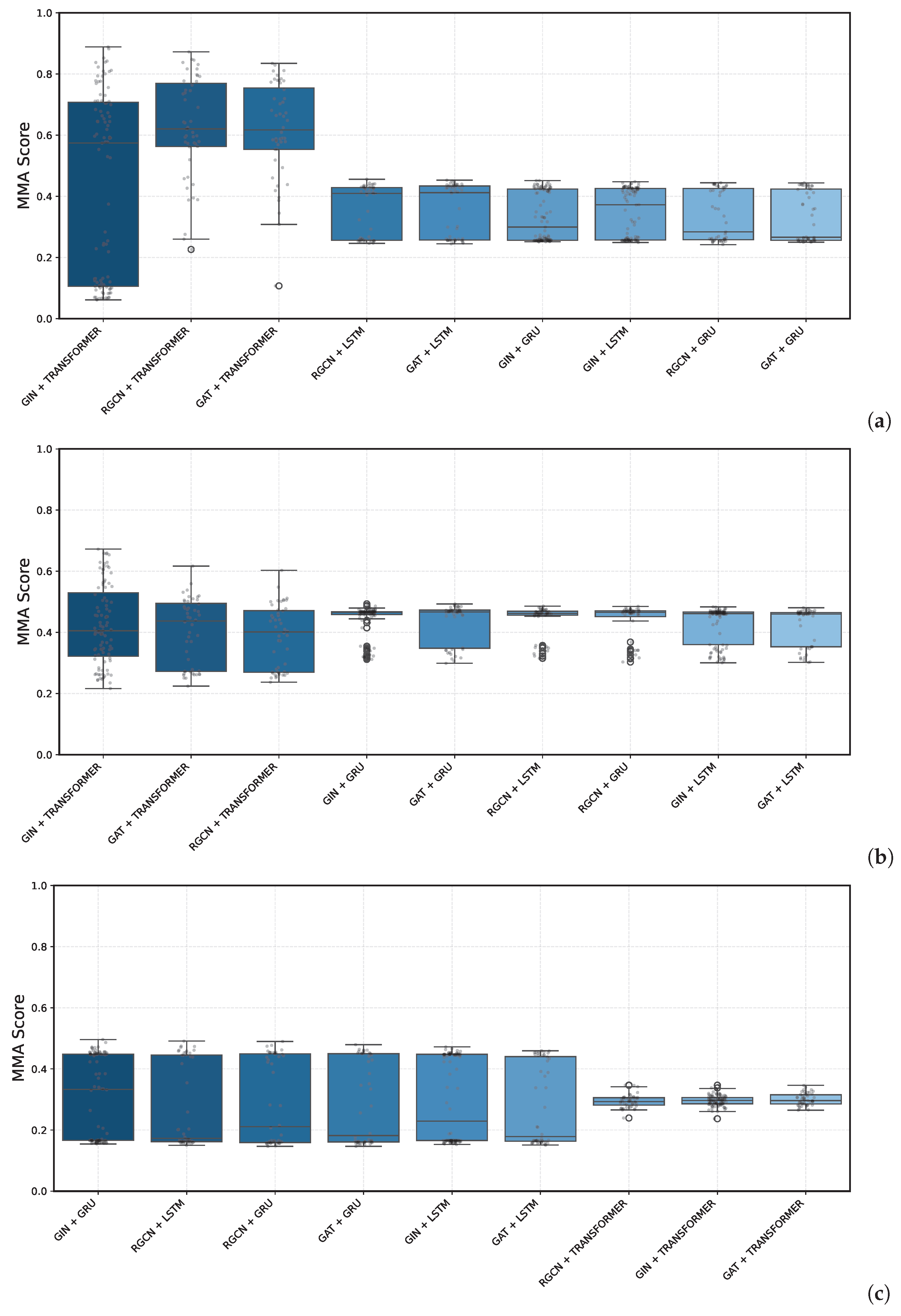
In our experiments, three clinical tasks are considered in a supervised learning setting with labels extracted as described in Section 2.3. For each task, we first perform a grid search of model configurations on a held-out set of 154 patients to evaluate the impact of architectural choice. The grid spans three embedding dimensions (30, 100, 300), four graph encoders (GCN/GAT/RGCN/GIN subset), three sequence decoders (GRU, LSTM, Transformer), and varying network depths (1, 3, 5, 10 layers for both encoder and decoder), resulting in over 570 configurations, as shown in Figure 6. Each point in the plot corresponds to the maximum mean accuracy (MMA) between AUPRC and AUROC scores per configuration. The best configuration based on the MMA scores is selected for the main results, as shown in

Table 5. Best hyperparameter configurations for each clinical prediction task based on the highest maximum mean accuracy (MMA). The table reports the task, embedding dimension, encoder, encoder layers, decoder, encoder layers, MMA score, and average training time per epoch.

Task	d	Encoder	Layers	Decoder	Layers	MMA	Time (s)
Diagnosis	300	GIN	5	Transformer	5	0.89	4.68
Readmission	30	GIN	3	Transformer	3	0.66	1.39
Mortality	30	GIN	1	GRU	5	0.50	0.57

. Average training time is also reported in seconds per epoch.

For the main results, the remaining data are partitioned in 80/20 train–test splits at the patient level, preventing information leakage across patient trajectories, for a total of 8000 training and 2000 test patients (excluding 154 validation patients). All models are trained for 100 epochs using the Adam optimizer (lr = 0.001) and on an NVIDIA A100 GPU system, repeated over five runs with random initialization. We use a feature dimension size of 32 for text and numerical embeddings, and hidden dimensions of 512 and 128 in all encoders and decoders, respectively, with a dropout value of 0.2. The encoder output dimension is set to 256, and, 4 attention heads are used in case of GAT and transformers. All other encoder and decoder parameters are set as default.

State-of-the-art methods for clinical prediction for comparison in this work are selected, which rely on deep sequential models, attention mechanisms, and graph-based learning to capture the temporal and structural complexity of EHRs. As a sequence-based architecture, Dipole [10] employs bidirectional recurrent neural networks to model patient visit sequences, and RETAIN [9] introduces a reverse-time attention mechanism to improve interpretability while predicting clinical outcomes. Among other sequential methods, HiTANet [11] incorporates hierarchical time-aware attention to capture irregular time intervals between visits, while StageNet [13] leverages LSTM-based architectures to explicitly model disease progression stages. Other methods focus on adaptive feature extraction and patient similarity learning, such as AdaCare [12], which dynamically recalibrates clinical features, and GRASP [14], which learns patient representations by exploiting similarities across patient trajectories. Additionally, ManyDG [17] uses variational autoencoders to improve generalization across clinical tasks.

More recent approaches increasingly integrate external knowledge and graph structures; CGL [15] and KGxDP [16] represent codified data as patient knowledge graphs for reasoning and further incorporate clinical notes to enhance diagnosis prediction; however, these do this without an explicit learnable time component or numerical integration. The approaches in TCEM [21] and KCIF [19] adopt temporal heterogeneous graphs to capture interactions among medical entities and numerical values extracted from patient health knowledge graphs; however, these do this without textual side information. Temporal and context-driven predictions using relate-aware transformers and large language models (LLMs) are further explored in HEART [18] and DemGraph [20], respectively; however, these do this without an explicit time-dependence component.

Collectively, these methods demonstrate a variety of design options toward hybrid frameworks that combine knowledge-aware graph learning, multi-type integration, and temporal modeling to better represent the complex, multi-relational structure of healthcare data. The details of which specific components are included among these methods in terms of Learnable Temporal Component (LTC), task coverage (Diagnosis, Readmission, and Mortality), multi-modal input integration (Codified, Numerical, and Textual), Knowledge Graph capability for reasoning (KG), and Uncertainty Quantification (UQ) are shown in

Table 6. Comparison of healthcare prediction models across learnable temporal component (LTC), diagnosis (${\mathit{D}}_x$), readmission (${\mathit{R}}_x$), and mortality (${\mathit{M}}_x$) coverage, context integration (codified, numerical, and textual), knowledge graph support (KG), and uncertainty quantification (UQ). For each model, the presence of a corresponding component is check marked.

Model	Dx	Rx	Mx	LTC	Codified	Numerical	Textual	KG	UQ
RETAIN	✓	–	–	–	✓	–	–	–	–
Dipole	✓	–	–	–	✓	–	–	–	–
HiTANet	✓	–	–	✓	✓	–	–	–	–
AdaCare	–	–	✓	–	–	✓	–	–	–
StageNet	–	–	✓	✓	✓	✓	–	–	–
GRASP	✓	–	✓	–	–	✓	–	–	–
CGL	✓	–	–	–	✓	–	✓	✓	–
KGxDP	✓	–	–	✓	✓	–	✓	✓	–
ManyDB	–	✓	–	–	–	✓	–	–	–
HEART	✓	✓	✓	–	–	✓	✓	–	–
KCIF	✓	–	–	✓	✓	✓	–	✓	–
DemGraph	–	✓	–	–	–	–	✓	✓	–
TCEM	✓	–	–	✓	✓	–	–	✓	–
SeqGNN	✓	✓	✓	✓	✓	✓	✓	✓	✓

.

The results in

Table 7. Comparison of Sequential Graph Neural Network (SeqGNN) against state of the art (SOTA) reported in the literature in terms of area-under-receiver-operator-curve (AUROC), area-under-precision-recall-curve (AUPRC) and F1-score over five independent runs (mean values are shown with standard deviation in parenthesis). Paired t-distribution confidence interval (CI) is calculated in terms of AUPRC or F1, with respect to the proposed method. The best and second best results in each case are boldfaced and underscored, respectively.

Task	Model	AUROC	AUPRC	CI (%95)
Mortality (Mx)	RETAIN	59.4 (1.50)	9.6 (0.60)	(10.1, 12.2)
	AdaCare	58.4 (1.40)	11.1 (0.40)	(9.65, 10.7)
	GRASP	59.2 (1.40)	9.90 (1.10)	(9.54, 12.9)
	StageNet	61.5 (0.70)	12.4 (0.30)	(8.14, 9.20)
	ManyDG	66.3 (0.52)	14.1 (0.54)	(6.45, 8.23)
	SeqGNN (ours)	55.1 (0.56)	20.7 (0.60)	-
Readmission (Rx)	HEART	67.7 (0.79)	64.1 (1.46)	(3.73, 8.12)
	RETAIN	64.1 (0.70)	65.1 (0.10)	(3.03, 4.24)
	AdaCare	65.7 (0.30)	68.6 (0.60)	(1.68, 3.38)
	GRASP	66.3 (0.60)	66.3 (0.40)	(0.03, 1.18)
	ManyDG	68.6 (0.52)	67.0 (0.54)	(1.35, 3.13)
	DemGraph	73.9 (0.40)	68.7 (0.40)	(−1.34, 0.79)
	SeqGNN (ours)	71.5 (0.30)	68.5 (0.60)	-
Dataset	Model	AUROC	F1 Score	CI (%95)
Diagnosis (Dx)	DIPOL	82.1 (0.29)	70.4 (0.21)	(8.37, 8.94)
	RETAIN	83.2 (0.26)	71.3 (0.17)	(7.74, 8.40)
	HiTANet	82.8 (0.35)	71.9 (0.29)	(7.23, 7.67)
	KGxDP	86.6 (-)	74.7 (-)	-
	CGL	85.7 (0.16)	72.7 (0.10)	(6.28, 6.64)
	TCEM	86.7 (0.10)	73.1 (0.19)	(5.91, 6.22)
	KCIF	87.5 (0.12)	75.7 (0.22)	(3.36, 3.53)
	SeqGNN (ours)	93.1 (0.19)	79.1 (0.10)	-

compare the proposed SeqGNN with the above state-of-the-art baselines across clinical prediction tasks. For mortality prediction (Mx), SeqGNN achieves the highest AUPRC (20.7), outperforming prior baselines in terms of precision–recall performance. In terms of AUROC, it scores lower than the best-performing baseline, ManyDG (66.3), with StageNet (61.5) as the second best. In readmission prediction (Rx), SeqGNN attains the best AUROC (71.5), improving over the previous best model ManyDG (68.6). It achieves comparable AUPRC (68.5), on par with DemGraph (68.7). For the diagnosis prediction task (Dx), SeqGNN achieves the highest AUROC (93.1) and F1-score (79.1), surpassing the previous best model KCIF (AUROC 87.5, F1 Score 75.7). Overall, these results demonstrate that SeqGNN consistently achieves competitive performance and generalization across multiple clinical tasks, with patient knowledge graph integration and trainable temporal components.

To further evaluate the impact of different text embedding methods, we conducted an experiment using the validation set with a lightweight SeqGNN, configured by a single graph encoder layer and a single sequence decoder layer, using a GIN encoder and a Transformer-based decoder, and a reduced embedding dimension of 30. Multiple embedding methods, including the sentence transformer (SenTrans) [30], Long-Document Transformer (longformer) [31], Word2Vec [32], and One–Hot encoding of data, were evaluated under identical training conditions. Performance was assessed using AUROC and F1 for diagnosis prediction, and AUROC and AUPRC for readmission prediction, with the results reported in

Table 8. Comparison of textual embedding methods, namely Sentence Transformer (SBERT), Long-document Transformer (LongFormer), Word2Vec, and 1-hot encoding of data, across diagnosis and readmission tasks. The results are reported as mean ± standard deviation. Cohen’s d is computed with respect to sentence transformer.

	HF Diagnosis			Readmission
Model	AUROC	F1	Cohen-d	AUROC	AUPRC	Cohen-d
SBERT	0.94 ± 0.00	0.67 ± 0.01	–	0.79 ± 0.06	0.89 ± 0.03	–
LongFormer	0.94 ± 0.01	0.59 ± 0.24	0.49	0.78 ± 0.06	0.86 ± 0.02	0.10
Word2Vec	0.93 ± 0.01	0.58 ± 0.22	0.60	0.74 ± 0.09	0.87 ± 0.04	0.64
1-Hot Encoding	0.91 ± 0.03	0.57 ± 0.17	0.79	0.72 ± 0.10	0.84 ± 0.05	0.83

as mean and standard deviation across five runs. These results demonstrate the advantage of using sentence transformer, with statistically significant improvements as measured via the Cohen’s d coefficient.

4.1. Uncertainty Quantification and Model Calibration

To evaluate the reliability of the graph neural network predictions for heart-failure diagnosis codes, we implement an ensemble-based uncertainty quantification framework. Ten independent models ($K=10$), each with identical architecture, were trained from different random initializations for 100 epochs each. Predictive probabilities on the held-out test set were collected across all ensemble members, enabling separate quantification of epistemic uncertainty (model disagreement) and aleatoric uncertainty (inherent data stochasticity). The results are detailed in the following subsections.

4.1.1. Ensemble ROC

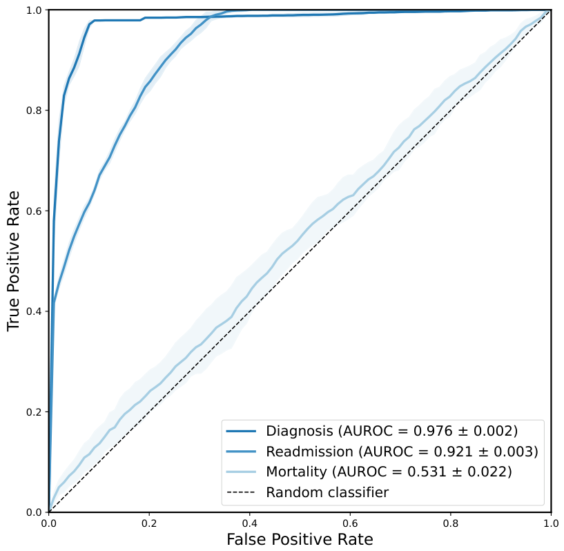
For each task, the AUROC curves are shown in Figure 7 using the 10-SeqGNN ensemble. It can be observed that for the task of HF diagnosis, the highest AUROC is reached at 0.97 with small cross-model variance. This suggests that the ensemble setting improves model confidence while increasing performance. A similar pattern is observed for 30-day readmission prediction where the SeqGNN members consistently perform determining the outcome given patient representations. In the case of mortality, however, high variance and low rates indicate uncertainty in predictions (close to a random classifier) among ensemble members and suggest the need for further tuning for practical usage.

4.1.2. Model Calibration

To evaluate whether the model reproduces the empirical mortality characteristics across diagnosis codes, a subgroup calibration analysis is performed [33]. First, the observed mortality rate is computed for each diagnosis code using the evaluation dataset. For a given code, the empirical mortality rate is defined as the proportion of admissions associated with that code that resulted in in-hospital death. The trained model is applied to the same evaluation set to obtain predicted mortality probabilities for each admission. For each diagnosis code, all admissions containing that code are grouped together, and the mean predicted probability of mortality across those admissions is calculated. This average predicted probability represents the model’s expected mortality rate for patients associated with that diagnosis code.

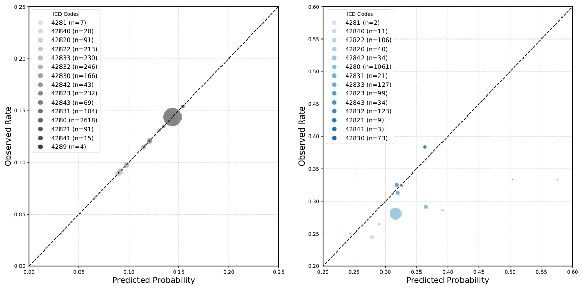
The calibration analysis, shown in Figure 8 (left), indicates that the model’s predictions are highly consistent with the observed mortality rates across HF diagnosis codes. For each ICD-9 code, the predicted rate (derived from model accuracy) closely matches the empirically observed mortality rate, with absolute errors close to zero. This implies that, at the diagnosis-code level, the proportion of predicted positive outcomes aligns almost perfectly with the true outcome frequency in the dataset. Furthermore, this pattern holds across common codes (e.g., 4280 with 2618 admissions) as well less frequent codes, suggesting stable calibration even when admission counts vary. Overall, these results indicate that the model’s probability estimates are well calibrated with respect to HF diagnosis groups; however, the model underpredicts for mortality task.

The calibration analysis for the readmission prediction model in Figure 8 (right) shows that for common ICD-9 codes with sufficient samples, the predicted accuracies are generally close to the observed readmission rates, indicating reasonable calibration. However, for rare codes with small counts (e.g., 42,821, 42,841, 4281), the model tends to over- or underpredict, leading to larger deviations from perfect calibration. Overall, the model demonstrates partial calibration, with reliable predictions primarily for the more frequent HF codes, while predictions for infrequent codes are less stable and overconfident.

Post hoc calibration was applied to assess the reliability of the model’s probability outputs, as shown in

Table 9. Effect of post hoc calibration methods on model performance across tasks in terms of expected calibration error (ECE) and area-under-precision-recall-curve (AUPRC).

	Diagnosis		Readmission		Mortality
Method	ECE	AUPRC	ECE	AUPRC	ECE	AUPRC
Uncalibrated	0.029	0.91	0.031	0.84	0.0210	0.111
Temperature Scaling	0.027	0.91	0.026	0.84	0.0009	0.112
Platt Scaling	0.018	0.91	0.027	0.84	0.0008	0.112

. For the diagnosis task, both Temperature Scaling and Platt Scaling yielded modest improvements in calibration, with Platt Scaling achieving the lowest ECE (0.018 versus 0.029 uncalibrated) while maintaining the same high AUPRC of 0.91. For the readmission task, calibration provided marginal benefits, reducing ECE from 0.031 to approximately 0.026–0.027, with no change in AUPRC (0.84). The most substantial improvement was observed for mortality prediction, where both calibration methods dramatically reduced ECE from 0.021 to below 0.001, accompanied by a slight increase in AUPRC from 0.111 to 0.112. Overall, these results demonstrate that post hoc calibration effectively improves probability calibration—particularly for more challenging tasks such as mortality prediction—without compromising discriminative performance learned through the patient knowledge graphs using SeqGNN.

4.1.3. Predictive Variance

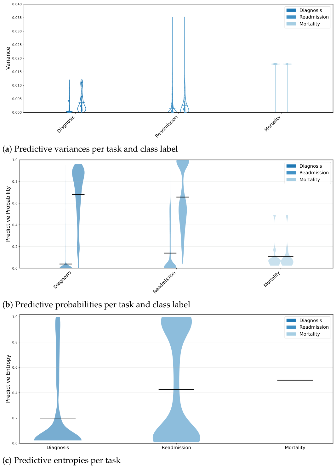
Epistemic uncertainty is assessed via predictive variance, defined as the sample variance of output probabilities across the 10 ensemble members for each test instance and diagnosis code. Variance distributions were visualized in Figure 9a, using kernel density estimate with and stratified by ground-truth label (positive vs. negative). Negative instances consistently exhibited low variance (mean ≈ 0.002–0.005), reflecting high ensemble agreement. Positive instances, which are far rarer in the test set, displayed moderately higher variance (mean ≈ 0.004–0.008), indicating greater model uncertainty when confirming specific heart failure phenotypes. The overall low variance magnitudes suggest reasonable model stability given the small cohort size.

4.1.4. Predictive Probability

The spread of predicted probabilities across ensemble runs provides direct insight into model confidence and output stability, as shown in Figure 9b. Probability distributions for negative instances were tightly concentrated near zero (mean ≈ 0.05–0.15), whereas positive instances received substantially higher mean probabilities (typically 0.6–0.8 for prevalent codes such as 4280 and 42821) for diagnosis and readmission tasks. Narrow distributions for the dominant code 4280 (present in all test samples), but wider spreads for rare subtypes, consistent with greater uncertainty on infrequent labels are observed. These patterns indicate that the ensemble produces conservative probability assignments for minority classes, which is clinically desirable but highlights the need for confidence-based filtering to improve.

4.1.5. Predictive Entropy

Aleatoric uncertainty as shown in Figure 9c, is quantified using predictive entropy, computed as the binary cross-entropy of the ensemble mean probability averaged over diagnosis codes for each test sample as follows:

$$H\left(\overline{p}\right)=-\overline{p}log\overline{p}-(1-\overline{p})log(1-\overline{p}),$$

where $\overline{p}$ is the mean probability across runs. It can be seen that the mean entropy values increases from diagnosis to mortality, consistent with above findings. Entropy thus complements variance by isolating irreducible data-driven uncertainty, offering clinicians a complementary signal for identifying cases that may warrant additional diagnostic review. The overall per-sample entropy values followed a unimodal distribution with mean ≈ 0.35 bits, indicating moderate intrinsic stochasticity in the heart failure cohort.

5. Discussion

In this section, we discuss the key findings of this study and provide answers to the three research questions (RQ) initially posed that examine the role of model design, confidence, and uncertainty in shaping the performance and reliability of SeqGNNs for clinical prediction tasks. Together, these analyses provide insight into not only how these models perform, but also how their behavior can inform model development and deployment in real-world clinical settings.

[RQ1]: Which components of sequential and longitudinal EHR modeling (temporal learning, multimodal fusion, and knowledge graph integration) are most influential for each clinical prediction task, and how effectively does a unified architecture combine these components across diagnosis, readmission, and mortality prediction? By comparing SeqGNN with a broad range of prior models that selectively incorporate temporal dynamics, modality-specific encoders, and knowledge graph structure, we can identify which modeling components are most effective for each clinical task and how well they transfer when unified in a single architecture.

For diagnosis prediction, the results show that strong performance is primarily driven by rich temporal modeling combined with structured knowledge graph integration, as SeqGNN achieves the highest MMA score of 86.1 (with AUROC 93.1 and F1 score 79.1), outperforming prior static, graph-enhanced and transformer-based models, indicating that fine-grained temporal dependency modeling is particularly critical for capturing diagnostic patterns. In this case, the second highest prior is achieved by KCIF, which uses patient graphs with MMA score of 81.6 (see Table 1), a decrease of 4.5 points in MMA, attributed to the lack of textual integration (see Table 6). Among prior models that do include an LTC, namely DIPOL, RETRAIN, and CGL, with MMA scores of 76.2, 77.2, and 79.2 respectively, undesirable decreases in performance for onset diagnosis prediction are observed. Among prior models that do not utilize patient knowledge graphs explicitly, HiTANet achieves the highest MMA score of 77.3, a further reduction of 8.75 points. TCEM, as a prior model that utilizes knowledge graphs representations, without textual or numerical integration, achieves an MMA of 79.9, signifying the added value from both knowledge graph and multi-modal integration. These findings highlight the importance of learnable MLP and integrated components combined with patient knowledge graph representations as proposed by SeqGNN.

For readmission prediction, similar improvements are observed associated with the integration of temporal progression modeling and patient-level structural context, where SeqGNN achieves the best AUROC (71.5) and remains competitive in AUPRC, suggesting the value in capturing longitudinal disease evolution and inter-event relationships. In particular, DemGraph, with a score of 71.3, exhibits a decrease of 2.35 in MMA due to the lack of an LTC. For mortality prediction, on the other hand, the most influential component appears to be multimodal signal integration, indicating that while structured and temporal components improve sensitivity to rare outcomes, mortality prediction remains highly sensitive to class imbalance and may require more specialized discriminative modeling. Overall, these findings show that temporal learning is beneficial, knowledge graphs enhance structured reasoning, and multimodal integration improves sensitivity in rarer outcomes. The proposed SeqGNN demonstrates that combining all components as such yields stronger generalization.

[RQ2]: What further insights do uncertainty and calibration analyses reveal about the reliability, limitations, and predictive behavior of the proposed SeqGNN architecture across clinical tasks? Uncertainty and calibration analyses provide a deeper understanding of model behavior beyond aggregate metrics, revealing where predictions are reliable and where limitations arise. Epistemic uncertainty, measured through ensemble variance, shows that the model is highly stable for negative cases and common diagnostic patterns, but exhibits increased uncertainty for positive and rare phenotypes, indicating that prediction difficulty is concentrated in clinically complex or underrepresented regions. Aleatoric uncertainty, captured via predictive entropy, further highlights that mortality prediction, with an entropic value around 0.5, is inherently more uncertain than diagnosis and readmission (see Figure 9), suggesting fundamental limits in predictability given the available data. Calibration analysis reinforces these findings: while diagnosis and readmission tasks are reasonably well calibrated—especially for frequent ICD-9 codes—mortality predictions show greater miscalibration and benefit significantly from post hoc correction (see Table 9). Overall, these analyses show that SeqGNN models are reliable in routine settings but less so in rare, high-risk scenarios, making uncertainty quantification an essential diagnostic tool for identifying model blind spots and guiding targeted improvements.

[RQ3]: To what extent can the relationship between encoder–decoder configurations, uncertainty, and performance inform future model deployment in decision support systems that rely on patient knowledge graphs and sequential modeling? The above findings highlight promising directions for leveraging confidence-aware modeling towards clinical deployment. Given that low correlations are present between patient records and outcomes based on the tasks studied in this work (see Figure 2), the addition of knowledge graph representation for patient visit trajectories is a recommended choice, as evident in the above analysis (see Table 1). Furthermore, various parameter settings and configurations are evaluated and found to be important in selecting final models (see Figure 6) as measured by the MMA scores on validation data. Such model variations combined with ensemble SeqGNNs strategies can be systematically incorporated into decision-making frameworks, such as deferring low-confidence predictions, prioritizing high-confidence cases, or integrating human-in-the-loop validation for uncertain outcomes. Further research is needed to investigate how confidence–performance relationships behave utilizing these methods in practice as well as under distribution shifts, class imbalance, and external validation cohorts, ensuring robustness in diverse clinical environments. Ultimately, these directions point toward the development of confidence-aware deployment strategies that enhance the safety, interpretability, and trustworthiness of clinical prediction systems.

6. Conclusions

In this work, we presented SeqGNN, a sequential graph neural network framework designed to model temporal patient trajectories within a heterogeneous clinical knowledge graph. By integrating graph-based representation learning with sequential modeling, the proposed approach captures both the structural relationships among clinical entities and the temporal evolution of patient visits. The model was evaluated on three clinically relevant prediction tasks—heart-failure onset diagnosis, 30-day readmission, and in-hospital mortality—using electronic health record data derived from the MIMIC-III database. The experimental results demonstrate that SeqGNN achieves state-of-the-art performance for diagnosis and readmission prediction while also providing considerable improvements in precision–recall performance for mortality prediction compared with several established baselines. In particular, the model achieved the highest AUROC and F1 score for diagnosis prediction, highlighting the benefits of jointly leveraging graph structure and temporal patient information. Future work will focus on incorporating additional clinical modalities such as clinical notes and imaging data and validating the proposed framework on larger and more diverse patient cohorts in a multi-center setting to further assess its robustness and generalizability in real-world clinical settings.