A Deep Learning Framework for Local Earthquake Magnitude Estimation Using Three-Component Waveforms

Abstract

This study presents a two-stage deep learning framework for accurate and generalizable estimation of local earthquake magnitudes from three-component seismic waveforms, within the context of ground-based remote sensing systems. In the first stage, phase transition boundaries are identified at the sample level to enable consistent temporal alignment of the signals. In the second stage, earthquake magnitude estimation is performed using 30 s waveform segments aligned with the early portion of the signal and enriched with spectral and statistical features. The model was initially trained on the globally diverse dataset STEAD and later fine-tuned using a subset of KOERI waveforms, and its performance was evaluated on an independent KOERI test set. The results demonstrate high prediction accuracy, with a mean absolute error of approximately 0.09 and a coefficient of determination (R²) of about 0.95, indicating strong agreement between predicted and true magnitudes. The model maintains stable performance across varying signal characteristics and geographic regions, highlighting its strong transferability. These findings suggest that seismic sensor networks can be effectively utilized as remote sensing systems for rapid and reliable earthquake characterization.

1. Introduction

In recent years, machine learning has demonstrated remarkable success across a wide range of domains, including medical imaging, natural language processing, speech recognition, finance, and signal processing [1,2,3,4,5]. Among these, deep learning approaches have proven particularly effective at extracting meaningful patterns from complex data, offering robust solutions to tasks where traditional methods often fall short.

Earthquakes are among the most devastating natural hazards, frequently resulting in significant loss of life and infrastructure. Their impact depends not only on magnitude but also on proximity to urban centers, local site conditions, and emergency response effectiveness. Consequently, rapid and accurate analysis of seismic waveforms plays a critical role in early warning systems and disaster mitigation strategies [6,7].

One of the most fundamental steps in seismological analysis is the accurate detection of P (primary)- and S (secondary)-wave arrivals in seismic recordings. These phase arrival times are essential for estimating key earthquake parameters such as epicenter location, origin time, and magnitude [7,8]. Similarly, rapid and reliable magnitude estimation supports damage assessment and enhances the efficiency of early warning mechanisms. While traditional approaches rely on empirical formulas involving peak amplitude, signal duration, or energy, machine learning models provide greater flexibility and generalization, particularly when trained on diverse datasets [9].

Machine learning applications aimed at extracting new insights from seismic data have advanced rapidly in recent years and have been successfully employed for various tasks in seismology. These tasks extend beyond phase picking and magnitude estimation, encompassing event location, signal classification, time prediction, and uncertainty modeling. For instance, Mousavi and Beroza [10] developed a Bayesian deep learning model to estimate earthquake locations using single-station observations.

CRED [11], designed for earthquake signal detection, combines CNN and GRU layers to perform robust detections even under low signal-to-noise ratio (SNR) conditions. EQTransformer [12] is a multi-task model that simultaneously performs phase picking and event detection within a unified architecture.

Accurate and automatic detection of P- and S-phase arrivals is crucial for estimating essential earthquake parameters such as location, origin time, and magnitude. In this context, PhaseNet [7] was one of the pioneering models to utilize a U-Net-style CNN architecture for phase picking. EQNet [13] extended this concept to multi-station data. Transformer-based approaches have also attracted attention in this domain. ViT-based models [14] demonstrated the superior generalization ability of self-attention mechanisms. Blockly Earthquake Transformer [15] was introduced as a customizable platform for phase identification. In addition, Capsule Network-based approaches [16] achieved high accuracy even with limited training data.

For automatic earthquake magnitude estimation, deep learning models generally use amplitude, duration, and frequency content of seismic signals as input. MagNet [17] performed direct magnitude estimation from three-component signals using a CNN and recurrent architecture, while transformer-based models [14] further improved estimation performance.

Beyond seismology, recent signal-based intelligent monitoring applications have increasingly emphasized the importance of domain adaptation, few-shot learning, and domain generalization strategies. In particular, deep learning models developed for varying operating conditions or limited-data scenarios have demonstrated robust performance and successful transferability to previously unseen environments [18,19]. These advances further highlight the importance of transferable and generalizable models for seismic applications, where regional and station-dependent variability can significantly affect signal characteristics.

Deep learning-based methods hold great promise for earthquake monitoring, phase picking, magnitude estimation, and early warning systems, representing a substantial advancement in computational seismology.

In this study, a two-stage deep learning approach is proposed for sample-level classification of P and S phases followed by local magnitude estimation using three-component seismic signals. The phase-picking model was trained on STEAD and applied to KOERI records, while the magnitude estimation model was fine-tuned and evaluated to assess its transferability and generalization capability.

The main contributions of this study can be summarized as follows:

• A two-stage deep learning framework combining seismic phase picking and local magnitude estimation;
• A hybrid feature integration strategy utilizing three-component waveforms, P–S arrival-time information, and handcrafted descriptors;
• A transfer learning strategy from STEAD to independent KOERI regional records;
• A systematic evaluation under different signal-to-noise ratio conditions to assess robustness in practical applications.

2. STEAD

The STanford EArthquake Dataset (STEAD) is a large-scale, globally distributed collection of high-quality seismic recordings, containing approximately 1.2 million three-component (E–N–Z) waveforms from 2613 stations worldwide between 1984 and 2018 [20]. Each waveform is 60 s long with 6000 samples per component and is accompanied by detailed metadata describing station coordinates, earthquake source parameters (latitude, longitude, depth, magnitude), P–S-phase arrival times, signal-to-noise ratio (SNR), and additional quality indicators. The dataset includes more than 450,000 local earthquakes and 100,000 noise-only signals, covering a magnitude range from –0.5 to 7.9, with most events being shallow and recorded within epicentral distances below 110 km.

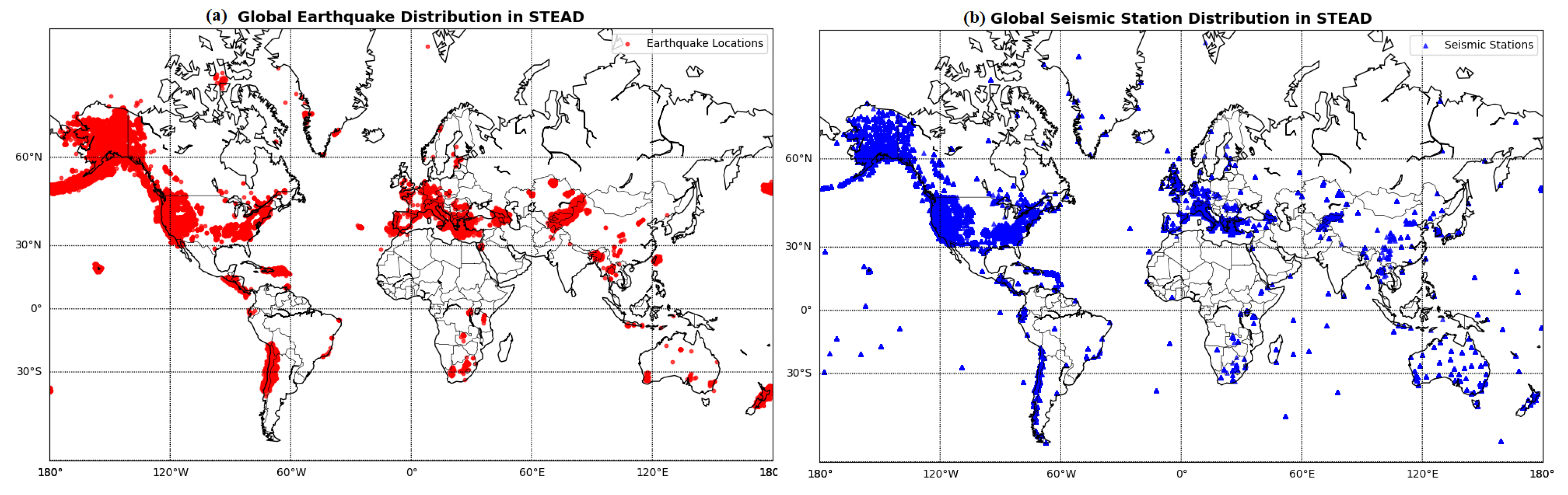
Figure 1a illustrates the global distribution of earthquake events included in STEAD, while Figure 1b shows the locations of the recording seismic stations.

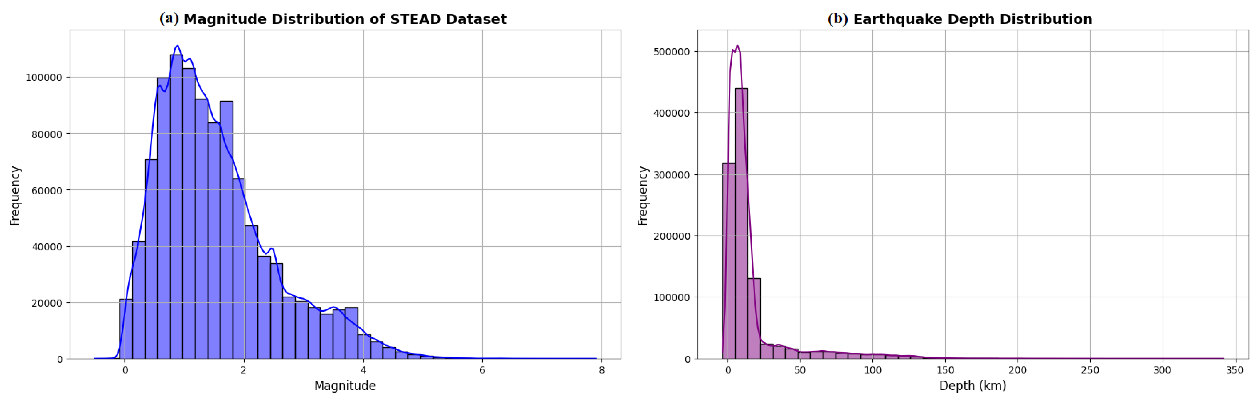
Figure 2a illustrates the magnitude distribution of earthquakes, highlighting that the majority fall within the 0–3 magnitude range. Figure 2b presents the depth distribution, where most events occur at depths shallower than 50 km.

Approximately 70% of P- and S-phase arrival times in the dataset were manually labeled by expert analysts [20]. The remaining picks were obtained from catalog phases and high-accuracy deep learning autopickers such as PhaseNet [7]. To enhance label reliability, the manual and automatic picks were cross-validated, and the CRED model [11] was used to remove out-of-catalog and multi-event records.

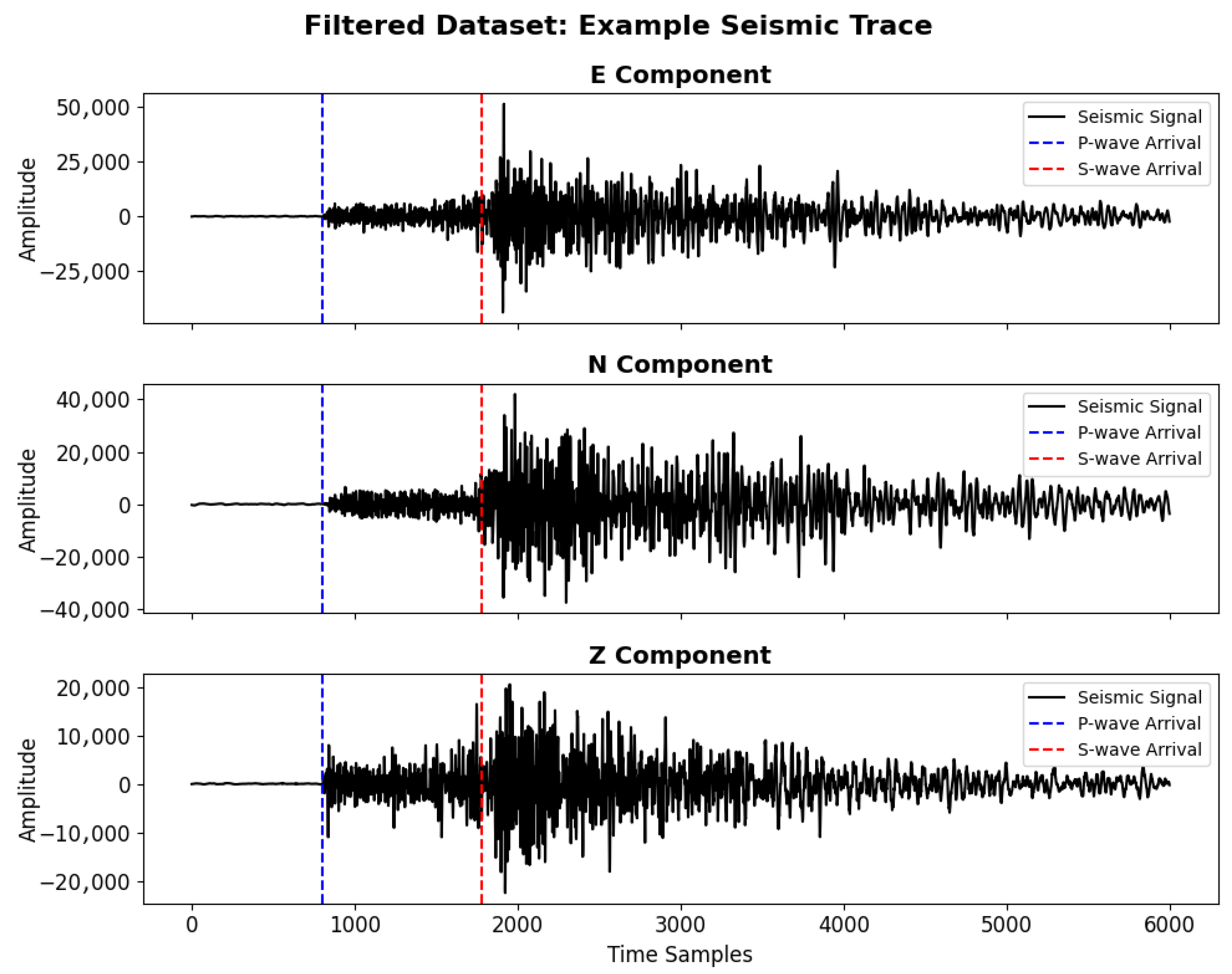
Figure 3 shows an example three-component waveform from the filtered dataset, where the blue dashed line marks the P-wave arrival and the red dashed line indicates the S-wave arrival.

With its extensive metadata structure and high-quality three-component recordings, STEAD provides a strong foundation for AI-driven seismic tasks such as event detection, phase picking, and magnitude estimation. In this study, multiple subsets of the dataset were extracted and used for model development.

3. P and S Arrival Time Estimation

This section presents the dataset, model architecture, and results related to the sample-level estimation of P- and S-wave arrival times using three-component seismic signals.

3.1. Data Preparation

A dataset of 50,000 high-quality seismic records was constructed for P–S-phase estimation. To ensure reliable measurements, only signals from local earthquakes (earthquake_local) with a focal depth > 0 km and a minimum three-component SNR ≥ 20 dB were retained. Records meeting these criteria were then stratified by magnitude to obtain a balanced distribution: events with M ≥ 3 and events with 0 ≤ M < 3 were sampled in equal proportion. This procedure resulted in a clean, magnitude-balanced dataset suitable for robust phase onset prediction.

3.2. Method

In this part of the study, a deep learning model was developed to estimate the arrival times of P and S waves at the sample level using seismic signals. The model performs phase classification by labeling each sample as noise, P-wave, or S-wave.

The input signals are 60 s long, corresponding to 6000 time samples, and include three components (Z, N, E). During the labeling process, each sample in a signal was assigned to one of three classes: noise (0) for the pre-P-wave segment, P-wave (1) for the interval between P and S arrivals, and S-wave (2) for the post-S-wave segment. Thus, the task was formulated as a multi-class time series classification problem at the sample level.

All signals were normalized using z-score normalization applied independently to each channel. The dataset was split into 70% training, 15% validation, and 15% test sets.

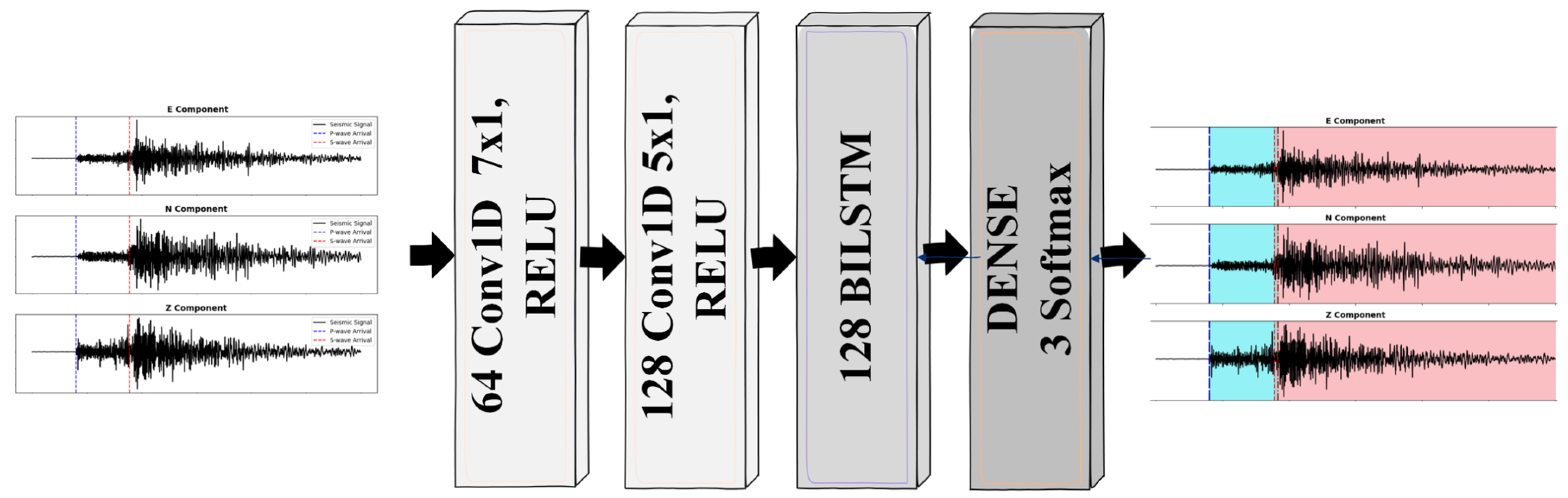
The model architecture is illustrated in Figure 4 and consists of the following three layers:

The overall functionality of the model is to process incoming seismic signals and identify the arrival times of P and S waves.

The proposed model consists of the following components:

• Input: The model takes three-component seismic signals (E, N, Z) as input.
• Feature Extraction: The first Conv1D layer (kernel size 7 × 1, 64 filters, ReLU activation) and the second Conv1D layer (kernel size 5 × 1, 128 filters, ReLU activation) are responsible for learning short-term spatial features from the input signals.
• Temporal Dependencies: A BiLSTM layer with 128 units captures bidirectional temporal relationships within the signal, enhancing the model’s understanding of sequence-level dependencies.
• Output: A Dense layer with softmax activation performs multi-class classification at each time step, assigning each sample to one of three classes: Noise, P-wave, or S-wave.

Through these stages, the model is capable of predicting the signal class at each time step, thereby allowing for accurate identification of P- and S-wave arrival times.

3.3. Results

The objective of the model is to accurately determine the arrival times of P and S waves at the sample level from seismic signals. To achieve this, each time step in the signal was classified into one of three categories: noise, P-wave, or S-wave, resulting in a multi-class time series classification task.

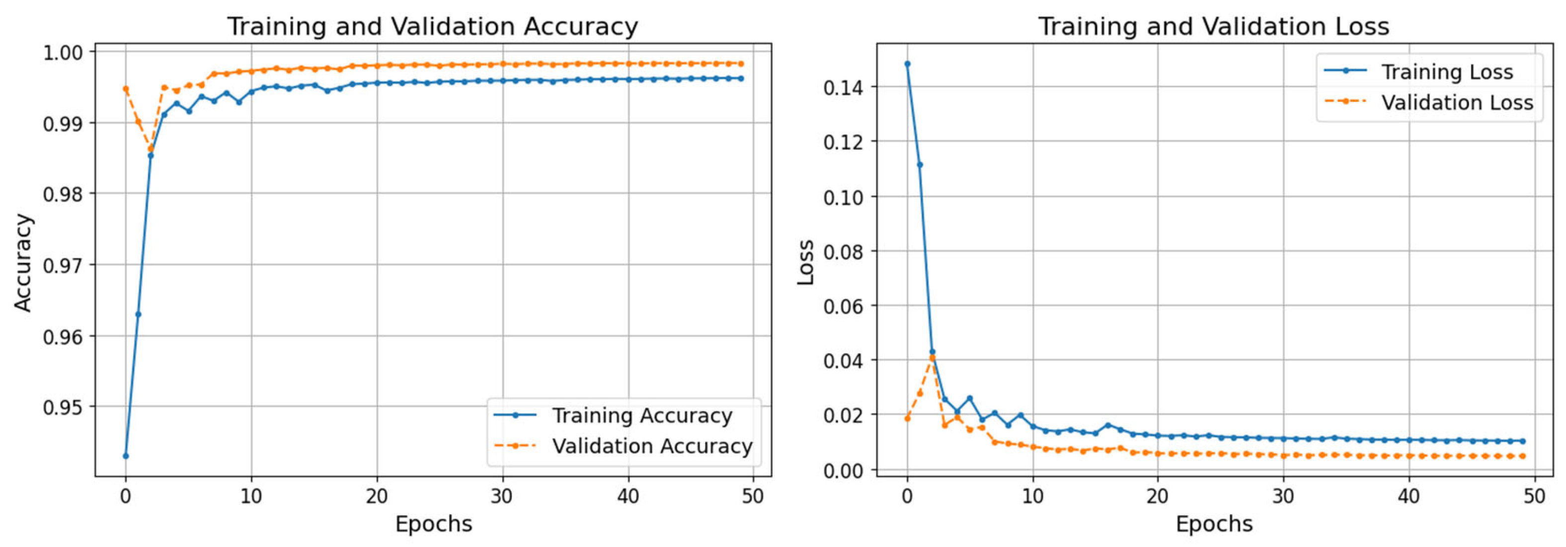
The model was trained for 50 epochs. Throughout the training process, the accuracy steadily increased while the loss values consistently decreased. These improvements observed on both the training and validation datasets indicate that the model successfully learned the phase classification task without exhibiting signs of overfitting.

The accuracy and loss curves for the training process are presented in Figure 5.

The output of the model is a sequence of class labels assigned to each time sample in a given signal, where each sample is classified as 0 (noise), 1 (P-wave), or 2 (S-wave). However, in the transition regions between phases, short-term label inconsistencies may occur in the classification results.

To mitigate such fluctuations and ensure more stable phase transitions, a simple decision rule was applied: class transitions were only accepted when at least five consecutive samples belonged to the same class. This threshold was selected to reduce short-term class fluctuations observed near phase transition boundaries. Lower thresholds tended to produce unstable and spurious phase transitions, whereas higher thresholds could delay the estimated phase onset times. Therefore, a five-sample criterion was adopted as a practical compromise between transition stability and temporal precision. This post-processing step improved the consistency and physical plausibility of the predicted P- and S-wave onsets. The first valid sample satisfying this condition in each phase was considered the estimated arrival time.

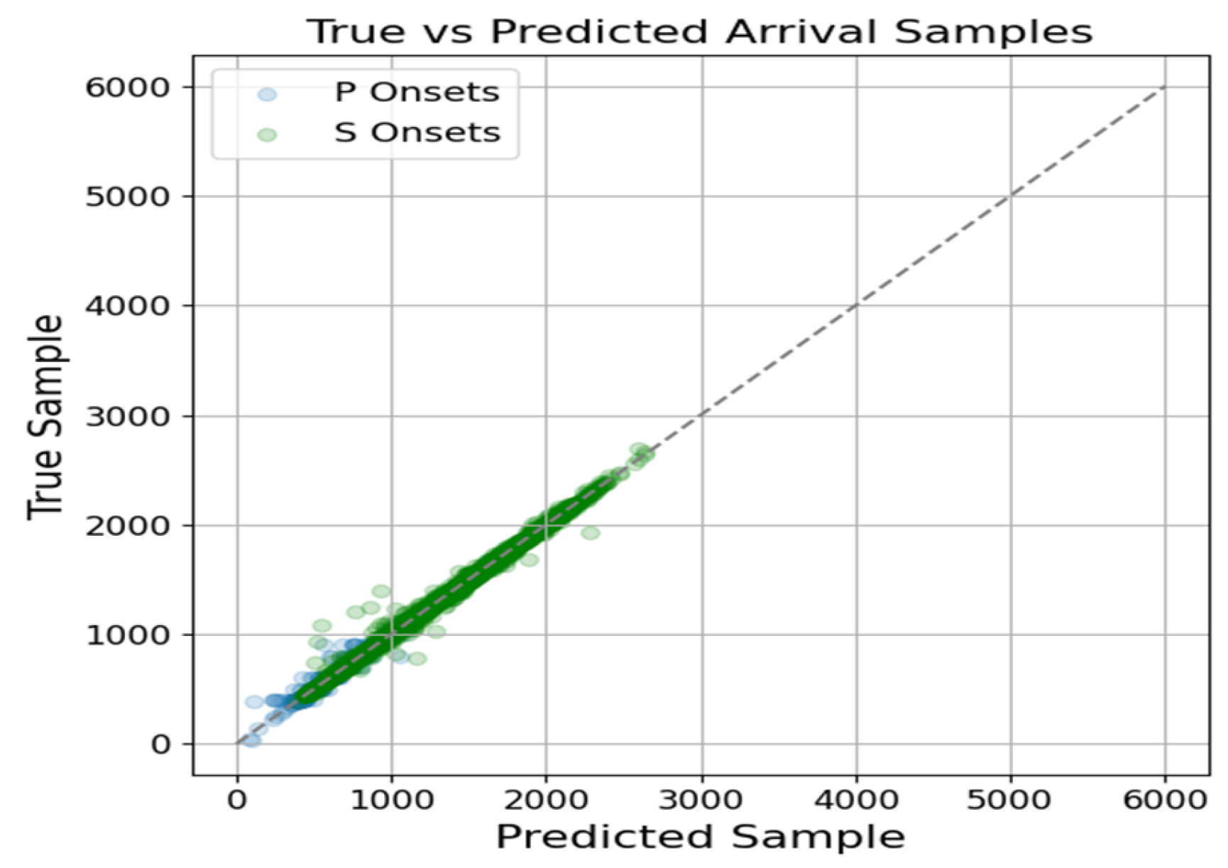
Figure 6 illustrates the relationship between the predicted and true arrival samples. Both P- and S-wave predictions are closely aligned with the reference line, indicating that the model is capable of estimating phase onsets with high accuracy.

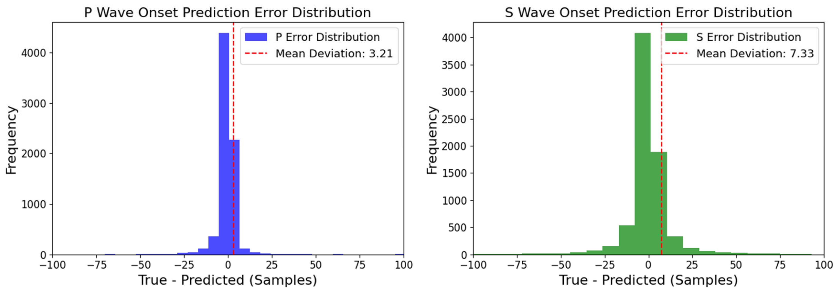
To evaluate how accurately the model predicts phase onsets, the error distributions are presented in Figure 7. The prediction errors for the P-wave are mostly concentrated within ±50 samples, whereas the distribution for the S-wave is broader. Nevertheless, the mean deviation for both phases remains close to zero.

The performance metrics calculated for the P and S phases are presented in

Table 1. Statistical performance metrics for the model’s P- and S-wave arrival time predictions on the test dataset.

Phase	MAE (Samples)	RMSE (Samples)	R2	MAPE
P	3.21	11.46	0.9957	0.58%
S	7.33	20.11	0.9975	0.65%

. For the P wave, the model achieved a mean absolute error (MAE) of 3.21 samples, a root mean square error (RMSE) of 11.46, an R² score of 0.9957, and a mean absolute percentage error (MAPE) of 0.58%. For the S wave, the corresponding values were 7.33, 20.11, 0.9975, and 0.65%, respectively.

These results demonstrate that the model achieves high accuracy with low error in predicting the arrival times of both seismic phases.

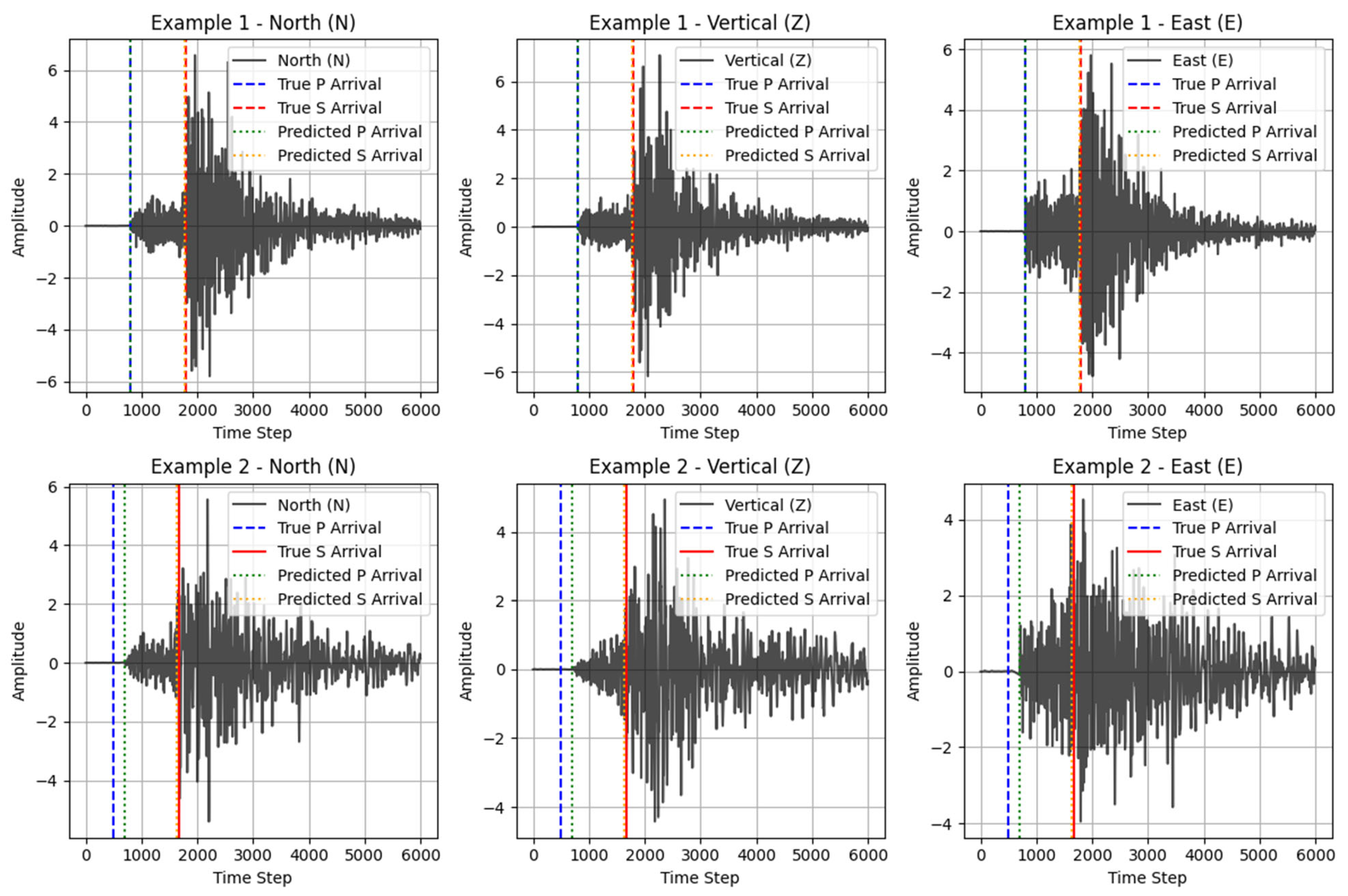
The phase prediction performance of the model at the signal level was examined using two representative earthquake events. In the visualizations presented in Figure 8, phase onset times are marked on the three-component waveforms—north (N), vertical (Z), and east (E)—for each seismic record. Blue and red dashed lines indicate the true P- and S-wave arrival times, respectively, while green and orange dotted lines represent the model’s predicted arrival times.

In the first example, the model successfully identified both P and S phases in close alignment with the amplitude structure of the signal. In the second example, a slight delay was observed in the S-phase prediction; however, the overall estimates remain physically consistent. These results demonstrate that the model is capable of phase separation regardless of signal characteristics and exhibits strong generalization ability across different events.

The sample-level prediction performance of the model was evaluated on five different earthquake examples selected from the test dataset.

Table 2. True and Predicted P- & S-Wave Arrival Times for Five Selected Earthquakes from the Test Dataset.

True P Arrival (Samples)	Predicted P Arrival (Samples)	True S Arrival (Samples)	Predicted S Arrival (Samples)
500.0	504	1307.0	1309
798.2	800	1676.2	1675
500.0	501	1318.0	1312
500.0	501	700.2	707
500.0	499	1064.0	1135

presents the true and predicted P- and S-wave arrival times for these five events.

As shown, the errors in P-wave predictions are generally limited to only a few samples, whereas more noticeable deviations can be observed in some S-wave predictions. Nonetheless, the overall alignment remains strong, indicating that the model is capable of producing consistent predictions across diverse signal characteristics.

In conclusion, the proposed model demonstrated high accuracy in estimating the arrival times of P and S waves at the sample level from seismic signals. Both the statistical performance metrics and the analyses conducted on individual waveform examples indicate that the model performs phase picking in a stable and consistent manner.

The low error values observed during training, along with the strong agreement on the test set, confirm the model’s ability to generalize across different signal types. These findings suggest that the developed approach can be effectively utilized in real-time seismic phase identification and earthquake characterization applications.

Although the employed model demonstrated strong performance in phase-arrival estimation, the main objective of this study is not phase picking but local earthquake magnitude estimation through a two-stage deep learning framework that jointly utilizes phase-arrival information and three-component seismic waveform data. In the literature, there are dedicated methods specifically developed for this task, such as PhaseNet [7], which have reported higher performance. Therefore, the phase-picking module was used as an auxiliary first-stage component supporting the subsequent magnitude estimation stage.

4. Machine Learning-Based Estimation of Local Earthquake Magnitudes

This section presents a machine learning approach for estimating the magnitude of local earthquakes using seismic signals. The model is designed to take as input a combination of time-series signals, the P–S-wave time interval, and various spectral and statistical features derived from the waveform. Rather than explicitly defining separate physical input variables for changes arising from different recording and propagation conditions, this study aimed to have the model learn such relationships in a data-driven manner through raw seismic signals and auxiliary features. The artificial neural network is trained and optimized specifically for events whose magnitudes are defined in terms of local magnitude (Ml).

4.1. Data Preparation

The earthquake magnitude estimation dataset was constructed from STEAD by applying the following filters to improve signal quality, metadata consistency, and station-level reliability: events with negative local magnitudes, which were extremely underrepresented in the source dataset, were excluded; records with focal depth > 0, source–receiver distance ≤ 110 km, minimum three-component SNR ≥ 20 dB, and labels of earthquake_local were retained. A total of 178,140 records satisfied these conditions. Furthermore, to ensure sufficient station representation, only stations with at least 2000 events were retained, resulting in a final dataset of 56,680 records.

Each record consists of three-component (Z, N, E) waveforms sampled at 100 Hz. The P and S arrival times provided in the dataset were used directly to compute the P–S interval, which was log-transformed for scaling. For each event, a fixed 30 s segment was extracted starting 1 s before the P-wave arrival (3000 samples total), consistent with previous STEAD-based magnitude estimation studies that also employed a 30 s P-referenced waveform window [14]. Shorter signals were zero-padded, and each channel was normalized using z-score standardization.

In addition to the waveform segment, 12 spectral and amplitude-based features (e.g., spectral entropy, RMS, dominant frequency) were extracted separately for each component. Three additional time-domain features derived from the P–S interval were included, forming a 15-dimensional feature vector for each record.

Spectral Entropy reflects the information content of a signal in the frequency domain based on the distribution of power across spectral components. After normalizing the power spectrum, Shannon entropy is calculated to quantify spectral irregularity. This approach is widely used to characterize and compare the frequency content of signals [21]:

$$H=-{\displaystyle \sum _{i=1}^n}{p}_{i}log\left(p_i\right)$$

(1)

where

p_i: Normalized power spectrum component;

n: Number of frequency bins.

Root Mean Square (RMS) is a fundamental statistical metric used to quantify the energy content of a seismic signal. RMS is calculated as the square root of the mean of the squared amplitudes. This measure is commonly used to assess the energy intensity of a time series and to enable comparison between different seismic records [22]:

$$RMS = \sqrt{{\displaystyle \frac{1}{n}} {\displaystyle \sum _{i=1}^n}{\left(xᵢ\right)}^2}$$

(2)

where

x_i: The i-th sample of the signal;

n: Total number of samples.

Peak Amplitude represents the maximum absolute amplitude value of a seismic signal. This feature is widely used to assess the strength and energy content of seismic events by identifying the signal’s highest amplitude. In particular, the maximum amplitudes of P and S waves play a critical role in estimating earthquake magnitude and analyzing source characteristics [23].

$$A_{peak}=max\left(\left|x_i\right|\right)$$

(3)

where

x_i: The i-th sample of the signal.

Dominant Frequency refers to the frequency component with the highest spectral amplitude in a seismic signal’s frequency spectrum [24]. This feature identifies the frequency range where the signal’s energy content is concentrated and serves as an important parameter in the characterization of seismic events. Dominant frequency is particularly useful for analyzing local site effects and source properties.

$$f_{dom}={argmax}_{f}S\left(f\right)$$

(4)

where

S(f): Spectral amplitude at frequency f;

f: Frequency (Hz).

Features extracted from the post-P-wave segment of seismic signals are widely used in magnitude estimation models [25]. One such feature is:

P–S Duration (PS Duration): Calculated as the difference between the sample indices of S- and P-wave arrivals.

$$D_{ps}=S_t-P_t$$

(5)

where

S_t: S time;

P_t: P time.

Logarithmic PS Duration: A logarithmic transformation was applied to the PS duration values to smooth the scale and reduce the impact of large amplitude ranges. For numerical stability, a constant value of 1 was added before applying the logarithm.

$$D_{ps}={Log(1+(S}_t-P_t\left)\right)$$

(6)

where

S_t: S time;

P_t: P time.

Total PS Energy: The total energy between the P- and S-wave arrivals is computed by summing the squared amplitudes of the signal samples in that interval.

$$E_{ps}={\displaystyle \sum _{n=p}^s}{\displaystyle \sum _{c=1}^3}{x}_{n,c}^2$$

(7)

where

x_n,c: Amplitude of the signal at sample n and channel c, where c ∈ {Z, N, or E}.

4.2. Method

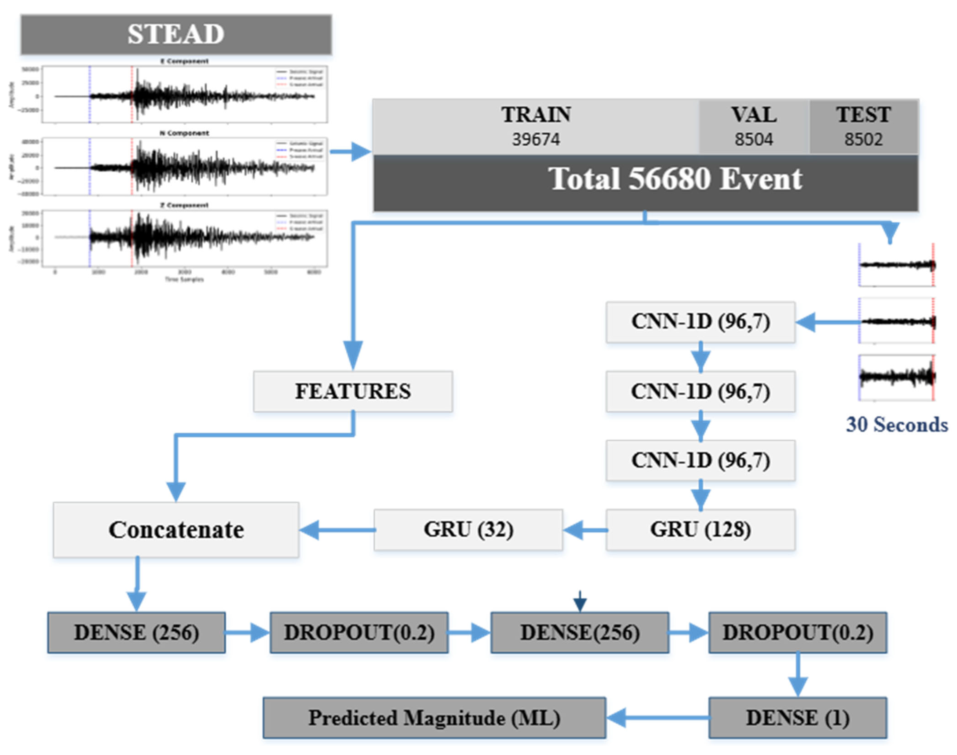
In this study, a multi-input deep learning model was developed for the purpose of earthquake magnitude estimation. The architecture of the proposed model is schematically illustrated in Figure 9. The framework was designed to combine automatically learned waveform representations with physically meaningful auxiliary descriptors in a unified regression model.

The primary input consists of three-component seismic signals (Z, N, and E), represented as fixed-length 30 s waveform segments. These signals are processed through a sequence of three Conv1D layers followed by two GRU layers. The convolutional layers are used to capture local waveform characteristics and frequency-related patterns, while the GRU layers model temporal dependencies and sequential relationships within the seismic traces.

The second input to the model is a 15-dimensional handcrafted feature vector extracted separately from the waveform data. This vector includes statistical, spectral, amplitude-based, and P–S-interval-related descriptors, providing complementary information to the deep features learned directly from raw signals.

The latent representation obtained from the waveform branch is concatenated with the handcrafted feature vector using a Concatenate layer. Following feature fusion, the combined representation is passed through two fully connected (Dense) layers with dropout regularization in order to improve generalization performance and reduce overfitting.

The final output layer consists of a single neuron with linear activation, producing the estimated local magnitude (ML) value.

The dataset was randomly divided into 70% training, 15% validation, and 15% test subsets. During partitioning, care was taken to preserve the overall magnitude distribution across all subsets.

All experiments were conducted in Google Colab using an NVIDIA A100 GPU environment with TensorFlow/Keras.

4.3. Results

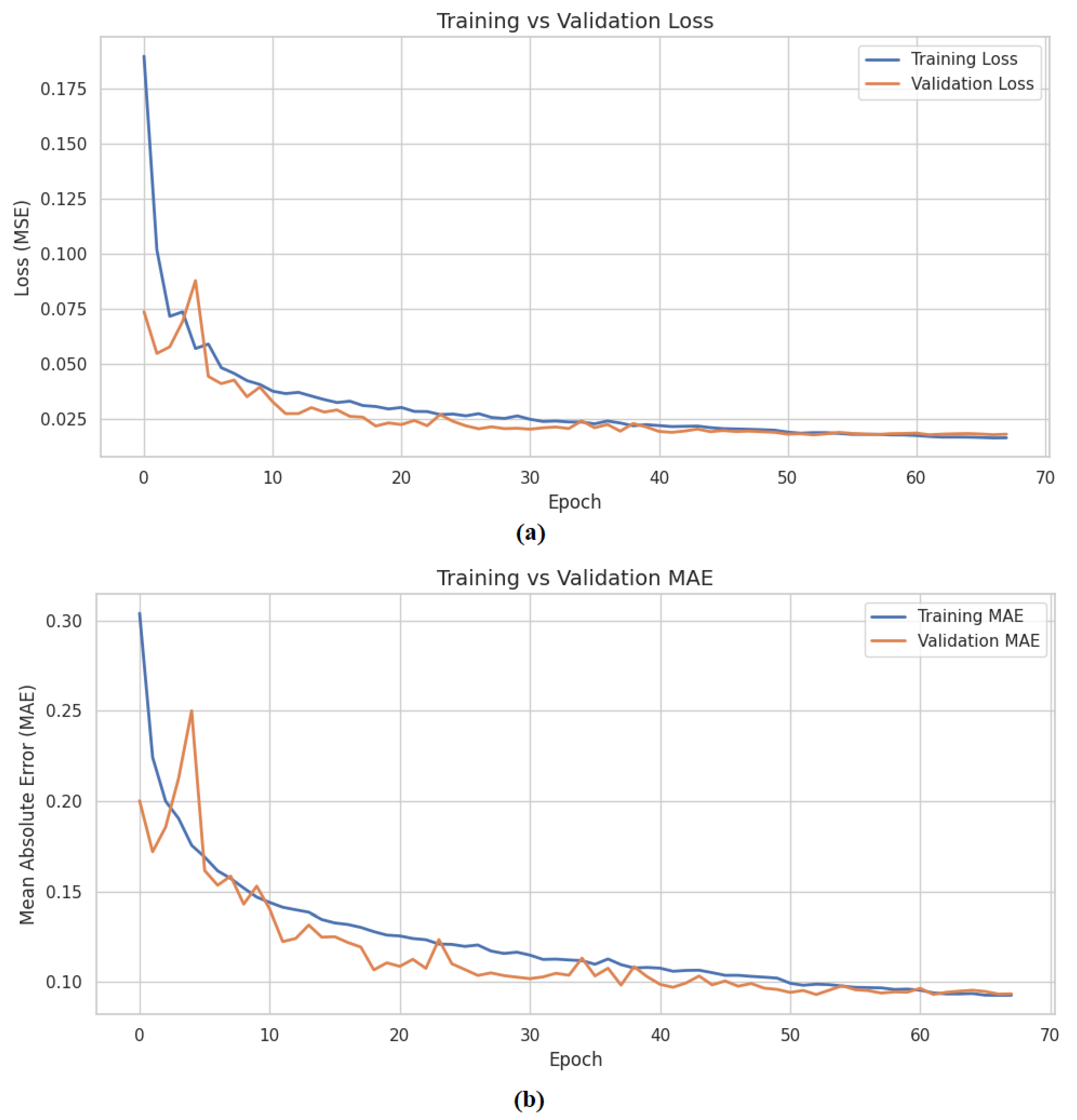
The epoch-wise evolution of the mean squared error (MSE) and mean absolute error (MAE) during training of the proposed model using the reference P–S arrival times provided in STEAD is presented in Figure 10a and Figure 10b, respectively. In both plots, separate curves are shown for the training and validation subsets.

As observed in Figure 10a, both training and validation losses decrease rapidly during the early epochs and gradually stabilize after approximately the 40th epoch, indicating successful convergence of the optimization process. The validation loss follows a trend similar to that of the training loss, suggesting satisfactory generalization behavior.

Similarly, the MAE curves shown in Figure 10b exhibit a steady decrease throughout training. Toward the final epochs, the validation MAE approaches approximately 0.09, indicating that the model can estimate earthquake magnitudes with relatively low absolute error.

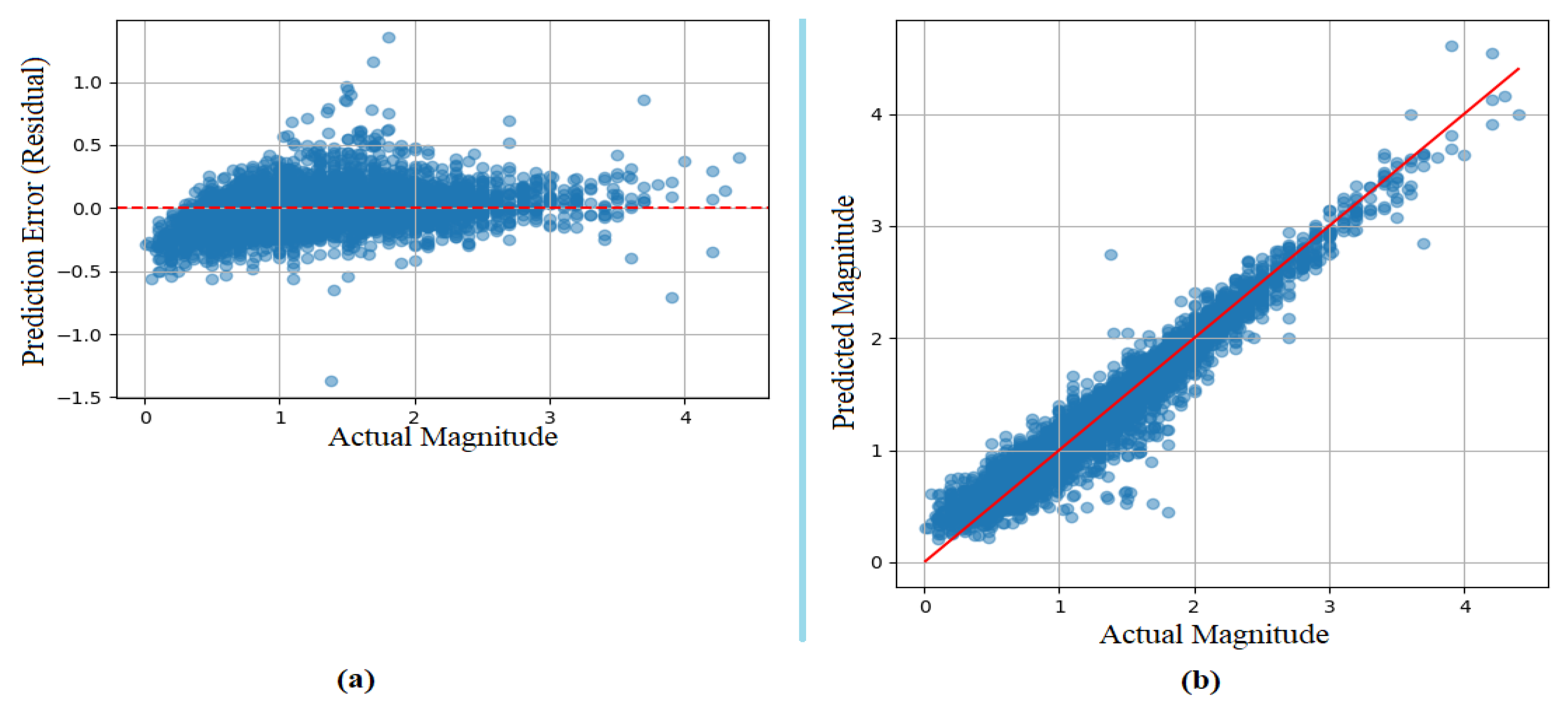
Figure 11 illustrates the prediction performance of the proposed model on the independent test set using the reference P–S arrival times. In Figure 11a, residual errors are plotted against the true magnitude values. The residuals are generally centered around zero across the evaluated magnitude range, indicating no pronounced systematic bias. A wider residual spread is observed for lower-magnitude events, whereas predictions become more concentrated at moderate and higher magnitudes. Only a limited number of scattered outliers are present. Figure 11b presents the scatter plot of predicted versus observed magnitudes. Most samples are distributed close to the reference line (y = x), demonstrating strong agreement between predicted and true values.

To further evaluate the robustness of the proposed framework against phase-picking uncertainty, the magnitude estimation model was additionally tested using both reference P–S arrivals and predicted P–S arrivals. The numerical performance metrics are summarized in

Table 3. Test performance of the proposed hybrid model using different phase-arrival sources.

Metric	Reference P–S Picks	Predicted Picks
Mean Absolute Error (MAE)	0.0920	0.0922
Mean Squared Error (MSE)	0.0170	0.0168
Root Mean Squared Error (RMSE)	0.1310	0.1294
Coefficient of Determination (R2)	0.9470	0.9481
Mean Absolute Percentage Error (MAPE)	10.95%	11.17%
Standard Deviation of Errors	0.1310	0.1294

.

The results show nearly identical performance under both settings. This finding indicates that the proposed framework maintains stable magnitude estimation performance even when predicted phase-arrival information is used instead of reference picks.

To further assess the contribution of each input component, additional experiments were conducted using different input combinations. Four model configurations were evaluated: (i) waveform only, (ii) waveform + P–S interval, (iii) waveform + handcrafted features, and (iv) the complete hybrid model. The comparative results are presented in

Table 4. Ablation study of different input configurations for earthquake magnitude estimation.

Model	Input Configuration	MAE	MSE	RMSE	R2
M1	Waveform only	0.0978	0.0195	0.1396	0.940
M2	Waveform + P–S interval	0.0966	0.0184	0.1356	0.943
M3	Waveform + Handcrafted Features	0.0976	0.0185	0.1360	0.943
M4	Waveform + P–S interval + Handcrafted Features	0.0920	0.0170	0.1310	0.947

.

The waveform-only configuration already yields competitive performance, indicating that the three-component seismic traces contain substantial information for magnitude estimation. Incorporating only the P–S interval leads to a modest improvement, whereas handcrafted features alone provide limited gains. The best overall performance is achieved when all input sources are jointly utilized. These findings suggest that waveform representations, arrival-time information, and engineered descriptors provide complementary information for local earthquake magnitude estimation.

4.4. Discussion

In this study, the proposed model for earthquake magnitude estimation was trained and tested using high-quality and geographically diverse records extracted from STEAD. Training samples were carefully selected based on criteria such as signal quality, availability of phase labels, and magnitude balance. The test set was constructed independently from random samples, without any geographic filtering, allowing for the evaluation of the model’s location-independent generalization capability. The resulting test performance (MAE: 0.092, RMSE: 0.131, and R²: 0.947) indicates that the model delivers high accuracy across the entire dataset. The obtained strong performance appears to benefit not only from a single input representation but also from the complementary use of multiple information sources, including three-component waveform signals, P–S arrival information, and handcrafted spectral/statistical descriptors.

In comparison, a Vision Transformer (ViT)-based model by Saad et al. [14] also performed magnitude estimation on STEAD data. That model achieved an MAE of 0.112 and standard deviation of 0.164 on the full STEAD test set, and slightly lower error on the Northern California (NCEDC) subset, with MAE: 0.079 and Std. Dev.: 0.120. However, despite being separated from the training set, the NCEDC test subset was geographically homogeneous, potentially limiting its generalizability.

Similarly, in the MagNet model proposed by Mousavi and Beroza [17], a CNN+LSTM-based architecture was employed to estimate magnitude using single-station waveforms. While the original study did not report the exact MAE, the standard deviation was stated to be approximately 0.2. Later, Saad et al. [14] re-trained this model and evaluated it on STEAD, reporting MAE: 0.141 and Std. Dev.: 0.219.

In another study using Complex CNN [26], the complex spectral representation of seismic signals (via STFT) was used, but higher error rates were obtained, with MAE reaching 0.26. These comparisons highlight that the model presented in this study offers a more explanatory, stable, and lower-error solution than existing methods—not only due to its input diversity but also due to its generalization strategy involving location-independent testing on STEAD. This suggests that the proposed model is not merely region-specific but has the potential to generalize across different continental seismic conditions.

Despite the favorable numerical performance, the obtained findings should be interpreted within the context of the adopted evaluation protocol. In this study, a random partitioning strategy was employed, which has been widely used in many previous deep learning studies in seismology. However, this scenario may be less restrictive than event-wise or station-wise separation protocols, where the model is evaluated on entirely unseen earthquake events or recording stations. In addition, previously reported studies may differ in terms of data partitioning strategies, sample sizes, data selection criteria, and preprocessing procedures. Therefore, numerical comparisons across different studies should be regarded as contextual performance references rather than strict one-to-one benchmarks. Consequently, although the proposed framework demonstrates competitive results under a methodology consistent with much of the existing literature, future validation using stricter partitioning strategies and additional regional datasets would provide a broader assessment of the model’s real-world generalization capability.

5. Evaluation of the Method Using the KOERI Dataset

In this section, the model trained on STEAD is evaluated using a completely different data source: the KOERI (Kandilli Observatory and Earthquake Research Institute) dataset. The aim is to analyze the model’s transferability and generalization capability on seismic records with different signal characteristics.

Before the evaluation, the STEAD-trained model was fine-tuned using a portion of the KOERI dataset to better adapt to regional signal characteristics, while a separate subset was reserved exclusively for independent testing.

To this end, three-component seismic waveforms corresponding to selected earthquakes from the KOERI catalog were retrieved via the IRIS web services and processed according to specific temporal and spatial criteria to construct an independent test dataset.

5.1. Earthquake Data Collection

Using the online query interface of KOERI, two distinct magnitude ranges were targeted:

• Earthquakes with ML ≥ 3.0 that occurred between 28 April 2020 and 28 April 2025.
• Small earthquakes with 0.0 ≤ ML < 3.0 that occurred between 28 April 2024 and 28 October 2024.

Merging the results of both queries yielded a total of 20,718 earthquake records. For nationwide coverage, the coordinates and operational time windows of 11 KOERI network stations were identified. Based on each event’s epicenter, stations located within a 110 km radius were selected. Earthquake–station matches were considered valid only when the station’s operational period overlapped with the earthquake occurrence time. After this filtering step, 6759 earthquakes were found to be suitable for station matching.

Seismic waveform data were retrieved using the IRIS web service, specifically requesting three-component records: HHZ, HHN, and HHE. For each matched event and station, a 70 s time window was defined, starting 10 s before the event origin time. Only records for which all three components were successfully retrieved were retained.

As a result, a total of 5922 complete three-component records were successfully assembled.

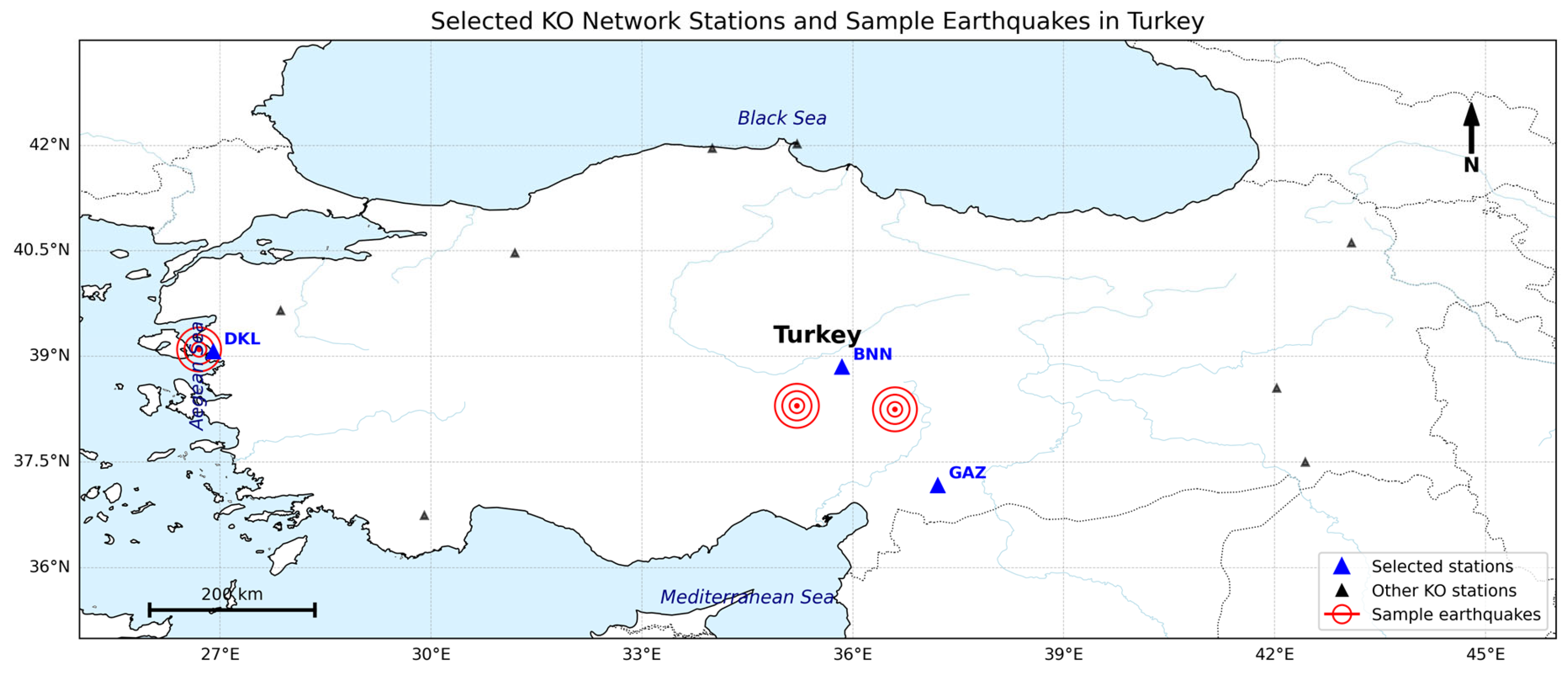
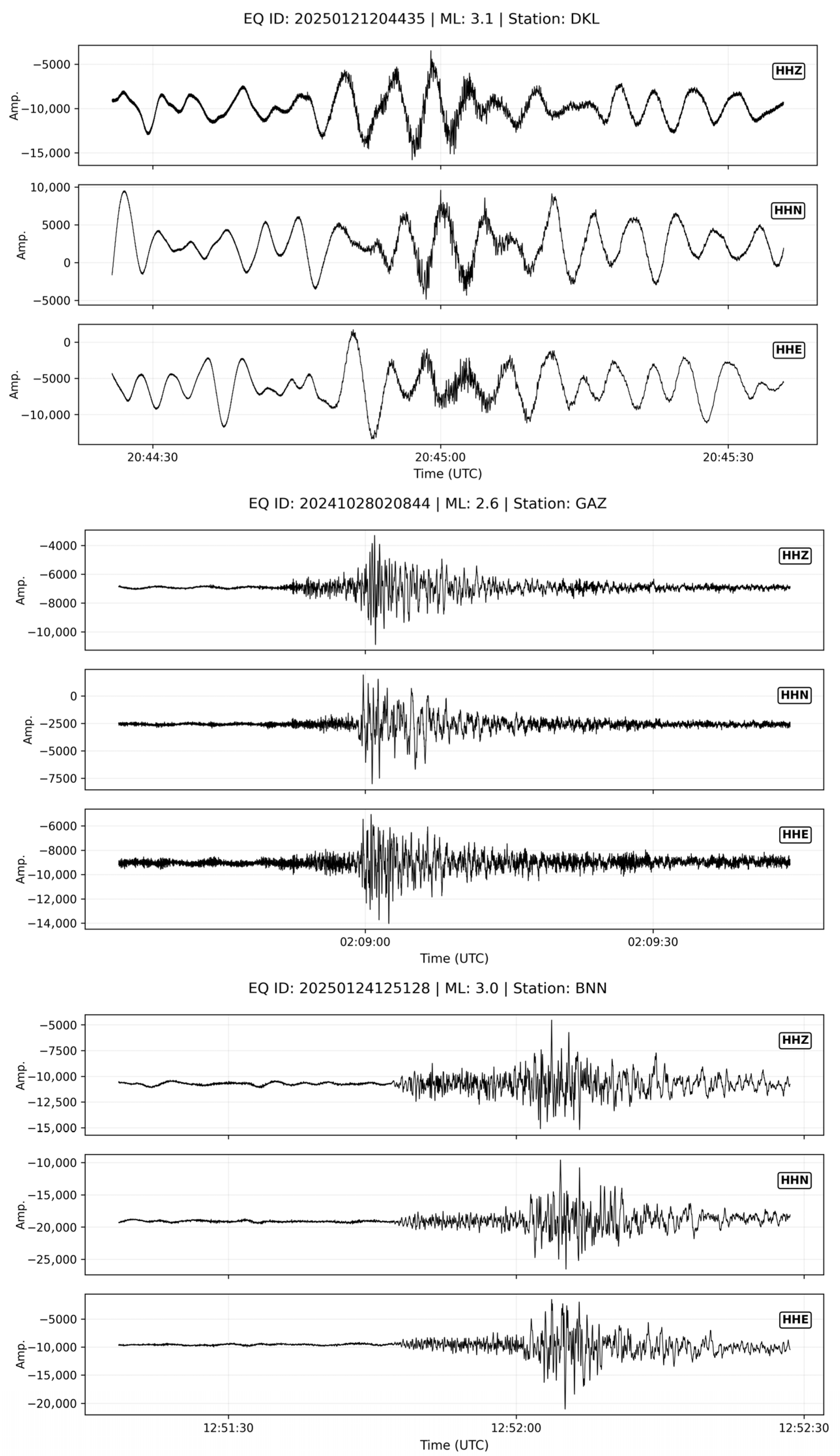
Figure 12 presents the spatial distribution of representative earthquake events selected from the KOERI dataset together with their corresponding recording stations. These examples were chosen to illustrate different magnitude levels and geographic regions within the study area.

• EQ ID: 20250121204435, an ML = 3.1 earthquake that occurred off the coast of the Edremit Gulf, was recorded by the DKL station.
• EQ ID: 20250124125128, an ML = 3.0 event near Göksun, Kahramanmaraş, was detected by the BNN station.
• EQ ID: 20241028020844, a small ML = 2.6 earthquake near İslahiye, Gaziantep, was recorded by the GAZ station.

For each of these stations, three-component seismic waveforms (HHZ, HHN, HHE) were retrieved using a 70 s window, starting 10 s before the origin time of the event. These waveforms are visualized in Figure 13 and were selected to highlight the diversity of signal characteristics and waveform structures present in the KOERI dataset.

To enable the estimation of P- and S-wave arrival times, all available .mseed records within the constructed KOERI dataset were provided as input to the model. However, some of these records contained incomplete or corrupted channel data, which rendered the prediction process technically infeasible for those cases. Following this initial screening, a total of 4914 earthquake records were identified in which both P and S arrival times were successfully predicted. These records were subsequently used in the final analysis of the model’s performance.

5.2. Estimation of P and S Arrival Times

The segmentation-based model trained on STEAD was applied in this study to predict the arrival times of P and S waves at the sample level from seismic signals in the KOERI dataset. The model operates as a multi-class time series classifier that assigns each time sample to one of three classes: noise, P-wave, or S-wave.

During the inference process, each 70 s three-component signal (HHZ, HHN, HHE) from KOERI was preprocessed using a 1–40 Hz bandpass filter, followed by channel-wise z-score normalization. These preprocessing steps were applied to ensure consistency with the training data and to enhance the clarity of the phase structures in the input signals [17].

The model’s output consists of a sequence of class probabilities corresponding to the three classes: noise (0), P-wave (1), and S-wave (2). To reduce classification ambiguity and stabilize phase transitions, a post-processing decision rule was applied. According to this rule:

• The first occurrence of at least five consecutive samples predicted as class 1 (P-wave) was identified as the P-wave onset.
• The S-wave onset was then determined as the first point after the P-wave where at least five consecutive samples were classified as class 2 (S-wave).

This decision logic suppresses noisy predictions caused by abrupt class fluctuations at the sample level and yields more physically consistent phase boundaries.

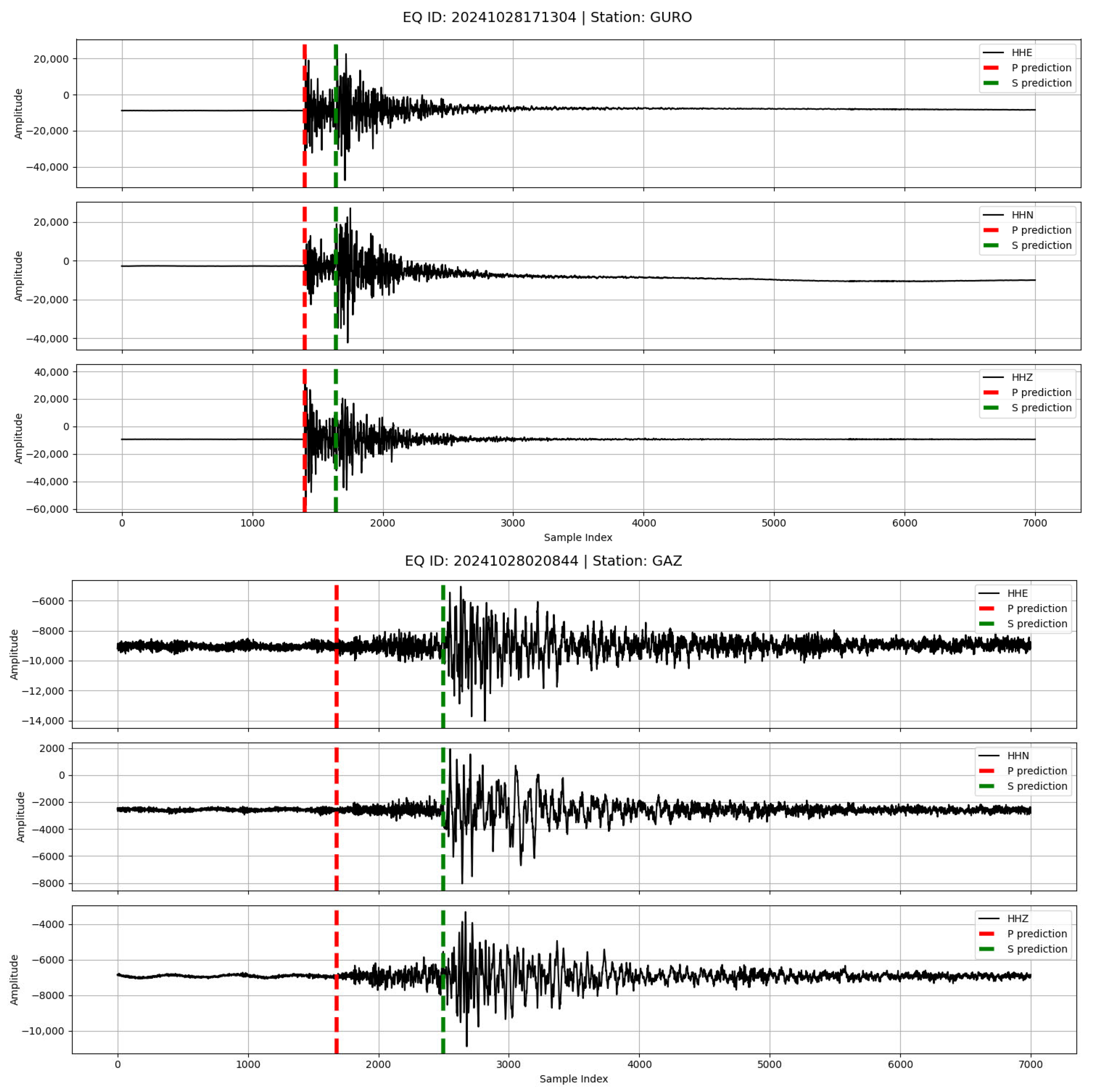
Figure 14 presents examples of the predicted P- and S-wave arrival times overlaid on three-component signals. The predictions are shown on signals filtered with the 1–40 Hz bandpass filter. Red dashed lines indicate the predicted P-wave arrivals, while green dashed lines denote the predicted S-wave arrivals.

Using this approach, the model-predicted values of P_start_sample and S_start_sample were calculated for each record and saved into a new CSV file. For each earthquake, only the signal from the first valid station was used to ensure consistency. Based on these predictions, the PS intervals, which form the foundation for phase separation analysis, were determined.

5.3. Signal-to-Noise Ratio (SNR) Calculation Method

In this study, seismic signals were subjected to several preprocessing steps prior to being fed into the model. As a first step, band-pass filtering between 1.0 and 40.0 Hz was applied to suppress high-frequency environmental noise and low-frequency displacement effects.

To assess signal quality and filter out low-quality examples from the training data, the signal-to-noise ratio (SNR) was calculated for each three-component (Z, N, E) seismic record. In this study, the SNR was computed separately for each channel, and the average of the three was used as the overall SNR value for the event.

The SNR is defined as follows:

$${SNR}_{avg}={\displaystyle \frac{1}{3}}{\displaystyle \sum _{c=1}^3}{SNR}_C$$

(8)

For each individual channel c, the SNR is defined as:

$${SNR}_C=10.{Log}_{10}\left(\frac{\frac{1}{L}{\sum }_{İ=1}^L{x}_{s,c}{\left[i\right]}^2}{max\left(\frac{1}{K}{\sum }_{İ=1}^K{x}_{n,c}{\left[j\right]}^2,\epsilon \right)}\right)$$

(9)

where

x_s,c[i] is ith sample of the signal window after the P-wave arrival in channel c;

x_n,c[j] is the jth sample of the noise window before the P-wave arrival in channel c;

L is the length (in samples) of the signal window;

K is the length of the noise window;

ε is a small positive constant used to prevent division by zero or near-zero values in the denominator.

This method was applied after the seismic signals were band-pass filtered within the 1–40 Hz frequency range. The computed average SNR values served as a quantitative indicator of signal quality.

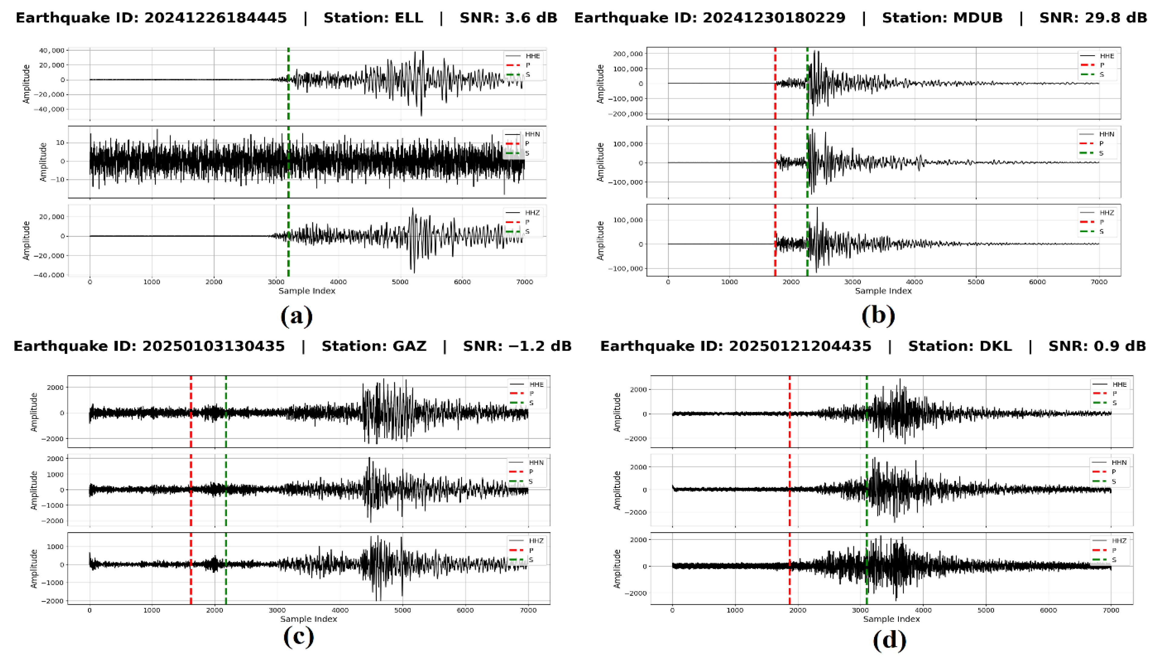
Figure 15 presents band-pass-filtered three-component seismic waveforms from four earthquake records with varying SNR levels, along with the model-predicted P- and S-phase onset times. The visualizations highlight how signal clarity and phase prediction reliability are affected by different levels of signal-to-noise ratio.

In the previous sections, a deep learning model trained on STEAD was introduced for estimating the magnitudes of local earthquakes using three-component seismic signals. In this section, the transferability and generalization capability of the model on an independent dataset, namely the KOERI records, are primarily evaluated through partial retraining (fine-tuning). In addition, the model was also directly tested without any fine-tuning, and noticeably lower performance was obtained. This finding highlights the importance of regional adaptation.

Experiments conducted with real-world field data assessed the model’s performance on records with varying levels of signal quality. Additionally, the quantitative impact of signal-to-noise ratio (SNR) on prediction accuracy was analyzed. The statistical distribution of KOERI records across different SNR ranges is summarized in

Table 5. KOERI dataset statistics across different SNR levels.

SNR Threshold	Num. of Records	Min ML	Max ML	AVG ML	AVG SNR
>0	3609	0.6	6.0	2.92	13.62
>5	2797	0.6	6.0	3.12	16.93
>10	2229	0.6	6.0	3.22	19.33
>20	940	1.0	5.6	3.40	25.27

.

The evaluation results obtained on the KOERI dataset across different SNR intervals are presented in

Table 6. Performance of the fine-tuned model on KOERI records across different SNR intervals.

SNR (dB)	N	Mean SNR	MAE	MSE	RMSE	R2	MAPE (%)
0–5	500	2.20 ± 0.06	0.254 ± 0.007	0.107 ± 0.003	0.327 ± 0.005	0.851 ± 0.004	13.58 ± 0.61
5–10	500	7.51 ± 0.03	0.208 ± 0.027	0.077 ± 0.018	0.276 ± 0.033	0.895 ± 0.024	9.17 ± 0.79
10–20	500	15.00 ± 0.05	0.173 ± 0.029	0.052 ± 0.017	0.225 ± 0.036	0.907 ± 0.034	6.20 ± 0.79
>20	500	25.21 ± 0.06	0.144 ± 0.002	0.042 ± 0.001	0.205 ± 0.003	0.912 ± 0.004	4.51 ± 0.12

.

Table 6 presents the results of controlled experiments conducted to evaluate the performance of the proposed model under different signal quality levels. The KOERI records were grouped into four distinct signal-to-noise ratio (SNR) bands: 0–5 dB, 5–10 dB, 10–20 dB, and above 20 dB. These intervals represent progressively increasing signal quality levels. In this way, model performance was examined in greater detail across varying noise conditions rather than relying on a single threshold value.

To ensure a fair and balanced comparison, 500 records were randomly selected from each SNR group as an independent test set. After excluding the test samples, all remaining records were divided into training and validation subsets and used for the fine-tuning stage. An 80%/20% training-validation split was applied. To reduce the effect of random sampling, the entire procedure was repeated using three different seed values (42, 123, and 2025), and all performance metrics were reported as mean ± standard deviation.

As shown in Table 6, model performance generally improved as signal quality increased. In the lowest-quality 0–5 dB group, the average values were MAE = 0.254, RMSE = 0.327, and R² = 0.851. In contrast, for the highest-quality above 20 dB group, the error values decreased and performance reached MAE = 0.144, RMSE = 0.205, and R² = 0.912. A similar gradual improvement was also observed in the intermediate bands.

The MAPE values followed the same trend. While the average percentage error was 13.58% in the lowest-SNR group, it decreased to 9.17% for the 5–10 dB interval, 6.20% for the 10–20 dB interval, and 4.51% for the above 20 dB group. This finding indicates that higher-quality seismic records yielded lower relative prediction errors.

Overall, the proposed two-stage deep learning framework produced consistent results across different signal quality levels and achieved lower prediction errors, particularly under higher-SNR conditions, for local earthquake magnitude estimation.

5.4. Real-Time Scenario and Independent Event Evaluation

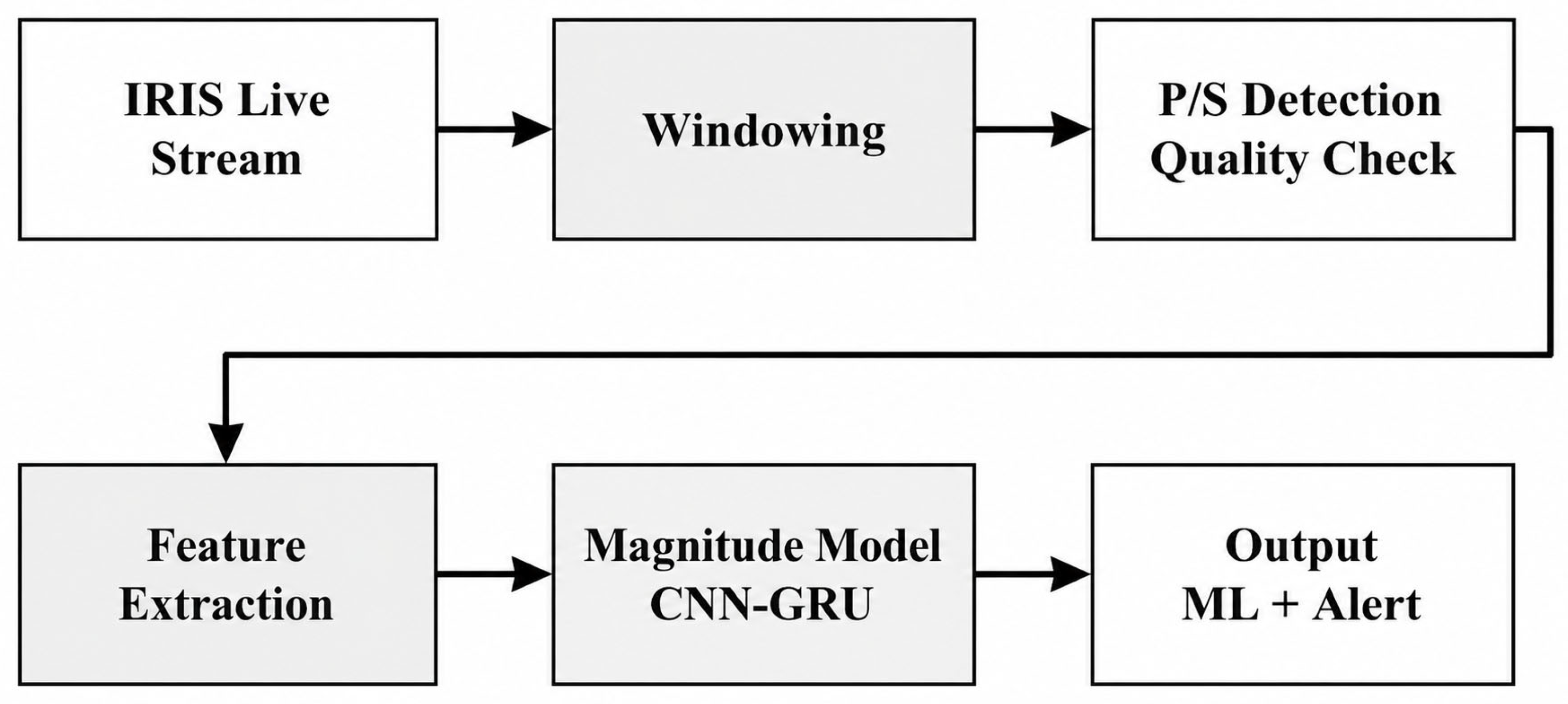
To demonstrate that the proposed system is applicable not only to offline datasets but also to operational environments, an additional end-to-end evaluation was conducted. The workflow presented in Figure 16 was designed according to a real-time monitoring scenario. In this framework, three-component seismic waveforms are automatically retrieved from the IRIS live seismic data services, segmented into fixed-length windows, processed for P- and S-phase arrival detection, subjected to signal quality control, transformed into feature representations, and finally provided to the CNN-GRU-based magnitude estimation model to generate local magnitude (ML) predictions. In this way, the system forms a sequential and fully automated earthquake monitoring pipeline without requiring manual intervention.

To evaluate the practical performance of this framework, independent earthquake events that were not used during the KOERI training or fine-tuning stages were selected. These earthquakes correspond to real catalog events that occurred at different dates and magnitude levels. The selected events are summarized in

Table 7. Independent KOERI earthquake events used in the real-time scenario test.

UTC Time	Region	True ML	Depth (km)
19 December 2025, 13:19:08	Goksun, Kahramanmaras	4.2	10.82
25 January 2026, 13:41:13	Pazarcik, Kahramanmaras	2.3	7.94
12 February 2026, 07:26:14	Pazarcik, Kahramanmaras	1.5	13.97
2 March 2026, 05:55:07	Pinarbasi, Kayseri	3.9	12.02
18 March 2026, 01:51:15	Ekinozu, Kahramanmaras	3.0	6.99

. For each event, waveform data corresponding to the catalog origin time were directly retrieved from the IRIS services, and the HHZ, HHN, and HHE components from the GAZ and BNN stations were automatically processed. For each record, a 70 s window starting 10 s before the origin time was used. This approach is consistent with the temporal windowing strategy adopted in the previous sections of this manuscript and reflects the system’s ability to generate rapid post-event magnitude estimates.

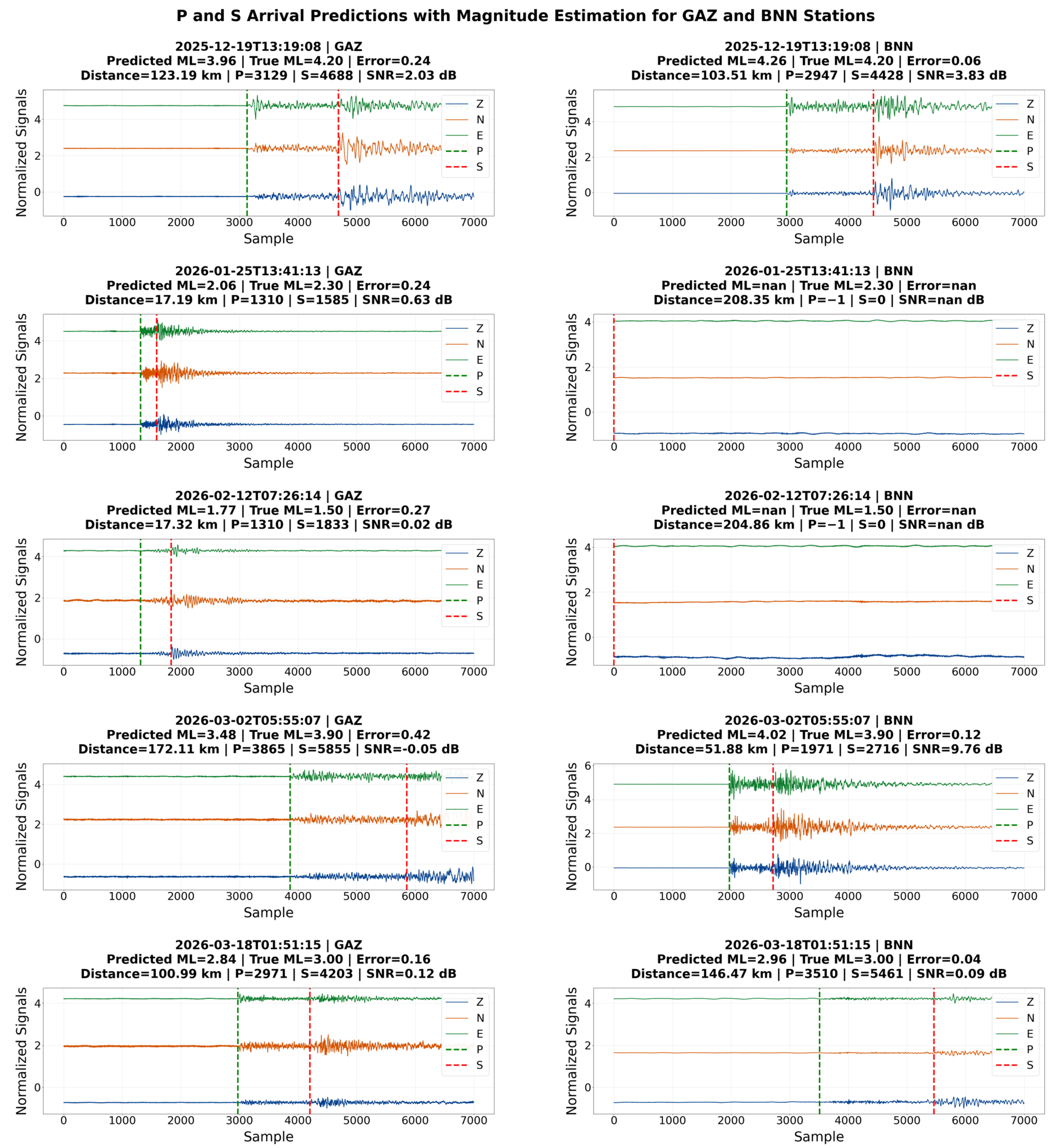
Figure 17 presents the three-component waveforms obtained from the GAZ and BNN stations for each selected event together with the model-predicted P- and S-wave arrival times, signal-to-noise ratio (SNR), epicentral distance, and magnitude predictions. Therefore, the figure illustrates not only numerical performance but also how the system operates directly on real seismic signals.

The results indicate that the model produces highly accurate estimates for records with sufficient signal quality. For example, for the Goksun earthquake of 19 December 2025, whose true magnitude was ML = 4.2, the model predicted 3.96 at the GAZ station and 4.26 at the BNN station. Similarly, for the Pinarbasi earthquake of 2 March 2026, whose true magnitude was ML = 3.9, the predicted values were 3.48 and 4.02, respectively. For the Ekinozu earthquake of 18 March 2026, predictions of 2.84 and 2.96 were obtained for the GAZ and BNN stations, both of which were very close to the catalog magnitude of ML = 3.0.

For smaller earthquakes and distant station records, the performance was observed to depend more strongly on signal quality. In the Pazarcik events with ML = 2.3 and ML = 1.5, the GAZ station was located approximately 17 km from the epicenter, and the model successfully produced predictions of 2.06 and 1.77, respectively. In contrast, the BNN station was located more than 200 km away from these events, where reliable separation of P and S phases could not be achieved; therefore, no valid magnitude estimate was generated. The “nan” outputs shown in Figure 17 correspond to these cases.

This experimental scenario reveals two important findings. First, the proposed system can operate automatically on real waveform records retrieved from a live seismic data source. Second, magnitude estimation performance depends not only on the model itself but also on physical recording conditions such as station distance, phase clarity, and signal quality. Overall, the obtained findings demonstrate that the proposed framework provides a practical and deployable structure that can be integrated into near-real-time earthquake magnitude monitoring systems under suitable station conditions.

6. Conclusions

In this study, a two-stage integrated deep learning framework was proposed for estimating both phase arrival times and earthquake magnitudes from local seismic signals. In the first stage, P- and S-wave arrival times were determined at the sample level using three-component seismic records. In the second stage, the obtained phase information was jointly utilized with raw waveform data and additional features for earthquake magnitude estimation. In this way, a practical framework integrating phase picking and magnitude estimation within a single operational pipeline was established.

Experimental results demonstrated that the proposed method achieved high accuracy with low error rates on STEAD. In addition, the model also produced effective results on KOERI records after fine-tuning, indicating that the proposed approach can be adapted to different regional and tectonic conditions. This finding supports that the framework is not limited to a single dataset but has a generalizable structure that can be applied across different seismic environments.

Additional analyses conducted under different signal-to-noise ratio levels showed that signal quality has a clear effect on magnitude estimation performance. In particular, lower error rates and higher prediction accuracy were observed under higher-SNR conditions. Nevertheless, the model also maintained stable performance on lower-quality records, further supporting its applicability under real-world field conditions.

Overall, the proposed two-stage approach provides promising results in terms of accuracy, robustness, and regional adaptability. Therefore, it may be considered an effective candidate method for real-time earthquake monitoring systems, rapid magnitude estimation applications, and automated seismological analysis platforms. Future studies may include the use of datasets from broader geographic regions, additional validation under stricter data partitioning strategies, and integration with advanced phase-picking models.

References

1. Sanida, T.; Sanida, M.V.; Sideris, A.; Dasygenis, M. Optimizing Lung Condition Categorization through a Deep Learning Approach to Chest X-Ray Image Analysis. BioMedInformatics 2024, 4, 2002–2021. [Google Scholar] [CrossRef]
2. Elazab, A.; Wang, C.; Abdelaziz, M.; Zhang, J.; Gu, J.; Gorriz, J.M.; Zhang, Y.; Chang, C. Alzheimer’s Disease Diagnosis from Single and Multimodal Data Using Machine and Deep Learning Models: Achievements and Future Directions. Expert Syst. Appl. 2024, 255, 124780. [Google Scholar] [CrossRef]
3. van Aken, B.; Winter, B.; Löser, A.; Gers, F.A. How Does BERT Answer Questions? In Proceedings of the 28th ACM International Conference on Information and Knowledge Management (CIKM), Beijing, China, 3–7 November 2019; pp. 1823–1832. [Google Scholar] [CrossRef]
4. Kheddar, H.; Hemis, M.; Himeur, Y. Automatic Speech Recognition Using Advanced Deep Learning Approaches: A Survey. Inf. Fusion 2024, 109, 102422. [Google Scholar] [CrossRef]
5. Pławiak, P.; Abdar, M.; Acharya, U.R. Application of New Deep Genetic Cascade Ensemble of SVM Classifiers to Predict the Australian Credit Scoring. Appl. Soft Comput. 2019, 84, 105740. [Google Scholar] [CrossRef]
6. Tan, M.L.; Becker, J.S.; Stock, K.; Prasanna, R.; Brown, A.; Kenney, C.; Cui, A.; Lambie, E. Understanding the Social Aspects of Earthquake Early Warning: A Literature Review. Front. Commun. 2022, 7, 939242. [Google Scholar] [CrossRef]
7. Zhu, W.; Beroza, G.C. PhaseNet: A Deep-Neural-Network-Based Seismic Arrival Time Picking Method. Geophys. J. Int. 2019, 216, 261–273. [Google Scholar] [CrossRef]
8. Stein, S.; Wysession, M. An Introduction to Seismology, Earthquakes, and Earth Structure; John Wiley & Sons: Hoboken, NJ, USA, 2009. [Google Scholar]
9. Bergen, K.J.; Johnson, P.A.; de Hoop, M.V.; Beroza, G.C. Machine Learning for Data-Driven Discovery in Solid Earth Geoscience. Science 2019, 363, eaau0323. [Google Scholar] [CrossRef] [PubMed]
10. Mousavi, S.M.; Beroza, G.C. Bayesian Deep Learning Estimation of Earthquake Location from Single-Station Observations. IEEE Trans. Geosci. Remote Sens. 2020, 58, 8211–8224. [Google Scholar] [CrossRef]
11. Mousavi, S.M.; Zhu, W.; Sheng, Y.; Beroza, G.C. CRED: A Deep Residual Network of Convolutional and Recurrent Units for Earthquake Signal Detection. Sci. Rep. 2019, 9, 10267. [Google Scholar] [CrossRef]
12. Mousavi, S.M.; Ellsworth, W.L.; Zhu, W.; Chuang, L.Y.; Beroza, G.C. Earthquake Transformer—An Attentive Deep-Learning Model for Simultaneous Earthquake Detection and Phase Picking. Nat. Commun. 2020, 11, 3952. [Google Scholar] [CrossRef]
13. Zhu, W.; Tai, K.S.; Mousavi, S.M.; Bailis, P.; Beroza, G.C. An End-to-End Earthquake Detection Method for Joint Phase Picking and Association Using Deep Learning. J. Geophys. Res. Solid Earth 2022, 127, e2021JB023283. [Google Scholar] [CrossRef]
14. Saad, O.M.; Chen, Y.; Savvaidis, A.; Fomel, S.; Chen, Y. Real-Time Earthquake Detection and Magnitude Estimation Using Vision Transformer. J. Geophys. Res. Solid Earth 2022, 127, e2021JB023657. [Google Scholar] [CrossRef]
15. Mai, H.; Audet, P.; Perry, H.K.C.; Mousavi, S.M.; Zhang, Q. Blockly Earthquake Transformer: A Deep Learning Platform for Custom Phase Picking. Artif. Intell. Geosci. 2023, 4, 84–94. [Google Scholar] [CrossRef]
16. Saad, O.M.; Chen, Y. Earthquake Detection and P-Wave Arrival Time Picking Using Capsule Neural Network. IEEE Trans. Geosci. Remote Sens. 2021, 59, 6234–6243. [Google Scholar] [CrossRef]
17. Mousavi, S.M.; Beroza, G.C. A Machine-Learning Approach for Earthquake Magnitude Estimation. Geophys. Res. Lett. 2020, 47, e2019GL085976. [Google Scholar] [CrossRef]
18. Zhao, H.; Liu, C.; Dang, X.; Xu, J.; Deng, W. Few-Shot Cross-Domain Fault Diagnosis of Transportation Motor Bearings Using MAML-GA. IEEE Trans. Transp. Electrif. 2026, 12, 1165–1174. [Google Scholar] [CrossRef]
19. Li, J.; Deng, W.; Ding, J.; Zhao, H. IBN-MixStyle Network With Dynamic Weighted Invariant Risk Minimization for Domain-Generalized Bearing Fault Diagnosis. IEEE Trans. Consum. Electron. 2025, 71, 9929–9939. [Google Scholar] [CrossRef]
20. Mousavi, S.M.; Sheng, Y.; Zhu, W.; Beroza, G.C. STanford EArthquake Dataset (STEAD): A Global Data Set of Seismic Signals for AI. IEEE Access 2019, 7, 179464–179476. [Google Scholar] [CrossRef]
21. Zhang, A.; Yang, B.; Huang, L. Feature extraction of EEG signals using power spectral entropy. In Proceedings of the 2008 International Conference on BioMedical Engineering and Informatics (BMEI), Sanya, China, 27–30 May 2008; pp. 435–439. [Google Scholar] [CrossRef]
22. Oppenheim, A.V.; Schafer, R.W. Discrete-Time Signal Processing, 3rd ed.; Prentice Hall: Upper Saddle River, NJ, USA, 2010. [Google Scholar]
23. Zollo, A.; Lancieri, M.; Nielsen, S. Earthquake magnitude estimation from peak amplitudes of very early seismic signals on strong motion records. Geophys. Res. Lett. 2006, 33, L23312. [Google Scholar] [CrossRef]
24. Aftabi, M.; Motamedi, M.H.; Molladavoodi, H. A Study on Parameters Influencing Blast-Induced Frequency Content and Dominant Frequency Attenuation. Shock Vib. 2022, 2022, 4626536. [Google Scholar] [CrossRef]
25. Heidari, R. τps, a new magnitude scaling parameter for earthquake early warning. Bull. Earthq. Eng. 2018, 16, 1165–1177. [Google Scholar] [CrossRef]
26. Ristea, N.-C.; Radoi, A. Complex neural networks for estimating epicentral distance, depth, and magnitude of seismic waves. IEEE Geosci. Remote Sens. Lett. 2022, 19, 7502305. [Google Scholar] [CrossRef]
27. IRIS DMC. IRIS FDSN Web Services for Seismic Waveform and Metadata Retrieval [Dataset]. Incorporated Research Institutions for Seismology. 2024. Available online: https://service.iris.edu/fdsnws/ (accessed on 1 April 2026).
28. Çelik, Y. Earthquake Magnitude Estimation. Zenodo 2026. [Google Scholar] [CrossRef]
Figure 1. (a) Global distribution of earthquakes in the dataset. Red dots indicate earthquake epicenters. (b) Seismic station locations in the dataset, represented by blue triangles.
Electronics 15 02055 g001
Figure 2. (a) Magnitude distribution of earthquakes in STEAD. Most earthquakes are concentrated in the 0–3 magnitude range. (b) Depth distribution of earthquakes, with the majority occurring at depths shallower than 50 km.
Electronics 15 02055 g002
Figure 3. A three-component seismic waveform (E, N, Z) from the filtered dataset. The blue dashed line indicates the P-wave arrival time, while the red dashed line marks the S-wave arrival time.
Electronics 15 02055 g003
Figure 4. Proposed model architecture for P- and S-wave arrival time prediction. The model processes three-component seismic signals using Conv1D, BiLSTM, and Dense layers, classifying each time step as Noise, P-wave, or S-wave. The output highlights predicted P- and S-wave regions in blue and red, respectively.
Electronics 15 02055 g004
Figure 5. Training and validation performance of the proposed model. (Left) Accuracy of the model on the training and validation datasets across 50 epochs. (Right) Loss values for training and validation, showing rapid convergence and stability after a few epochs.
Electronics 15 02055 g005
Figure 6. Relationship between true and predicted arrival samples. Blue dots represent P-wave predictions, while green dots indicate S-wave predictions. The dashed line corresponds to perfect prediction accuracy (y = x).
Electronics 15 02055 g006
Figure 7. Sample-wise error distributions of arrival time predictions for the P wave (left) and S wave (right). The histograms show the differences between true and predicted arrival samples (True − Predicted). Red dashed lines indicate the mean deviation for each phase.
Electronics 15 02055 g007
Figure 8. Comparison of true and predicted P-wave (blue/green dashed lines) and S-wave (red/orange dashed lines) arrival times for two example earthquakes. The seismic signals are shown for the East (E), North (N), and Vertical (Z) components.
Electronics 15 02055 g008
Figure 9. Architecture of the proposed magnitude estimation model. The model processes three-component seismic signals and extracted feature vectors to estimate local magnitude (ML).
Electronics 15 02055 g009
Figure 10. Training and validation performance of the model across epochs: (a) Mean Squared Error (MSE), (b) Mean Absolute Error (MAE).
Electronics 15 02055 g010
Figure 11. Test set prediction performance. (a) Residuals plotted against actual magnitudes. (b) Scatter plot of predicted versus actual magnitudes, where blue dots represent individual test samples and the red line indicates the ideal prediction trend.
Electronics 15 02055 g011
Figure 12. Geographic distribution of the selected sample earthquakes and KO Network stations across Türkiye. Sample earthquake epicenters are illustrated with concentric red circles. Selected recording stations are shown as blue triangles and labeled with their station codes, while other KO stations are indicated by black triangles.
Electronics 15 02055 g012
Figure 13. Three-component seismic waveforms (HHZ, HHN, HHE) recorded for the selected earthquakes. Each signal spans 70 s, beginning 10 s prior to the origin time, and reflects different magnitudes and propagation characteristics.
Electronics 15 02055 g013
Figure 14. Model-predicted P and S arrival times shown on filtered three-component waveforms. Red and green dashed lines indicate the final P and S picks after applying the post-processing rule.
Electronics 15 02055 g014
Figure 15. Predicted P and S phases over bandpass-filtered three-component waveforms from earthquakes with varying SNR levels.
Electronics 15 02055 g015
Figure 16. Real-time workflow of the proposed earthquake magnitude estimation system.
Electronics 15 02055 g016
Figure 17. Prediction results for independent KOERI events at the GAZ and BNN stations.
Electronics 15 02055 g017