A Routing and Cache Management Framework Based on Adaptive Q-Learning for Marine Opportunistic Networks

Abstract

Marine opportunistic networks are characterized by highly dynamic topology, intermittent connectivity, and severe resource constraints. Traditional routing protocols that rely on fixed-parameter Q-learning cannot adapt to real-time network changes, leading to suboptimal performance. This paper proposes an adaptive framework with three novel contributions: (1) a dynamic learning rate that adapts to network scale, node load, and congestion; (2) a dynamic discount factor that adjusts according to message urgency, hop count, and node mobility; (3) a multi-dimensional reward function with sliding window weights to balance delay, hop count, and node reliability. An asynchronous double Q-learning structure further mitigates overestimation bias. Extensive simulations on the ONE platform demonstrate that the proposed integrated algorithm (IR-DQ) achieves a high delivery ratio, significantly outperforming Epidemic and Spray and Wait, while substantially reducing overhead compared to fixed-parameter Q-learning. The framework exhibits superior adaptability to dynamic marine environments.

1. Introduction

The ocean, covering approximately 71% of the Earth’s surface, is a vital domain for global trade, resource exploration, environmental monitoring, and national security. Maritime activities increasingly rely on efficient and reliable communication networks to support autonomous vessels, marine sensor networks, and offshore platforms. However, the unique characteristics of marine environments pose fundamental challenges to traditional communication architectures. Nodes such as ships, buoys, drones, and offshore platforms are sparsely distributed, highly mobile, and their trajectories are significantly influenced by natural factors including ocean currents and wind. Communication distances are long, signal attenuation is severe, links are intermittent, and network resources such as energy, storage, and bandwidth are strictly limited. These features render conventional network architectures based on stable end-to-end paths, such as TCP/IP, largely inapplicable in marine scenarios [1].

Opportunistic networks (OppNets) have emerged as a promising communication paradigm that does not rely on persistent connectivity [2]. By exploiting node mobility to create transient encounter opportunities, OppNets adopt a “store-carry-forward” mechanism that enables asynchronous multi-hop data transmission even in the absence of continuous end-to-end paths. This approach is particularly well-suited for infrastructure-poor or highly dynamic environments such as oceans, disaster areas, and remote regions. Despite its conceptual appeal, the practical deployment of OppNets in marine settings faces significant obstacles. The high dynamics of node mobility, the intermittent nature of connectivity, and the severe constraints on network resources collectively challenge the performance of existing routing protocols.

Over the past two decades, numerous routing protocols have been proposed for OppNets, each with distinct design philosophies and trade-offs. Epidemic routing [3] achieves high theoretical delivery ratios through a flooding-based approach but suffers from excessive redundancy and resource consumption. PROPHET [4] reduces unnecessary transmissions by leveraging historical encounter probabilities; however, its accuracy degrades rapidly when mobility patterns change unpredictably. Spray and Wait [5] bounds the number of message copies to control overhead but lacks intelligent copy distribution mechanisms that could further improve efficiency. More recent protocols such as MaxProp [6] and Bubble Rap [7] incorporate priority-based scheduling and social network analysis, respectively, but either require global information or rely on stable social structures that may not exist in purely random marine mobility scenarios. A common limitation across these approaches is their reliance on static rules or single-dimensional metrics, which fundamentally lack the adaptability required to cope with highly dynamic and resource-constrained marine environments.

In recent years, reinforcement learning (RL), particularly Q-learning, has attracted significant attention for solving sequential decision-making problems in dynamic environments [8,9]. By treating each network node as an autonomous learning agent, Q-learning enables adaptive routing decisions that maximize long-term communication utility through continuous interaction with the environment. This paradigm offers a promising alternative to rule-based protocols, as it allows nodes to learn optimal forwarding strategies without requiring a priori knowledge of network dynamics. However, applying standard Q-learning to marine opportunistic networks introduces several challenges. First, fixed learning rates and discount factors cannot adapt to rapidly changing network conditions such as node density, congestion, and mobility patterns. Second, conventional reward functions that consider only single metrics like delay or hop count are insufficient to balance competing performance objectives including delivery ratio, latency, and resource efficiency. Third, the overestimation bias inherent in standard Q-learning [10] can lead to suboptimal policy selection and routing oscillations. Fourth, cache management—a critical resource optimization aspect—is often treated independently from routing decisions, despite their strong coupling.

To address these limitations, this paper proposes an integrated adaptive Q-learning-based routing and cache management framework specifically designed for marine opportunistic networks. The main contributions of this work are fourfold:

• Dynamic parameter adjustment mechanism: We introduce adaptive learning rate and discount factor models that respond to real-time network conditions. The learning rate adapts to network scale, node load, and congestion level, while the discount factor dynamically adjusts based on message urgency, transmission progress, and node mobility.
• Multi-dimensional intelligent reward function: A novel reward function is designed using a sliding window mechanism to dynamically integrate delay, hop count, and node historical reliability, enabling adaptive trade-offs among multiple performance metrics based on recent network conditions.
• Asynchronous double Q-learning structure: We adopt an asynchronous double Q-learning architecture that mitigates overestimation bias and enhances algorithm stability through decoupled action selection and value evaluation.
• Priority-based dynamic cache management: A message priority evaluation model is constructed considering message urgency, degree of replication, encounter probability with the destination, and message size, along with a dynamic cache replacement strategy that optimizes limited storage resources in coordination with routing decisions.

Extensive simulations conducted on the ONE (Opportunistic Network Environment) platform [11] demonstrate the effectiveness of the proposed framework. The integrated algorithm achieves significant improvements over baseline protocols, including a 71.2% increase in delivery ratio compared to Epidemic and a 26.2% reduction in overhead compared to fixed-parameter Q-learning, confirming the value of adaptive mechanisms for reliable and efficient communication in marine opportunistic networks.

The remainder of this paper is organized as follows. Section 2 reviews related work on opportunistic network routing, reinforcement learning applications, and cache management strategies. Section 3 presents the proposed adaptive Q-learning routing framework with dynamic parameter adjustment. Section 4 introduces the intelligent reward function and double Q-learning optimization. Section 5 describes the dynamic cache management strategy. Section 6 presents experimental results and analysis. Section 7 concludes the paper and discusses future research directions. A list of symbols is provided in the Appendix A.

2. Related Work

2.1. Classical Opportunistic Network Routing Protocols

Early research on opportunistic networks produced several classic routing protocols with distinct characteristics. Epidemic routing [3] emulates disease propagation by having nodes exchange all un-stored messages upon encounter, achieving high theoretical delivery ratios at the cost of massive redundancy and resource consumption. PROPHET [4] improves upon this by predicting future encounter probabilities based on historical encounter patterns, selecting high-probability nodes for forwarding to reduce redundancy while maintaining adaptability to certain mobility patterns. Spray and Wait [5] adopts a two-phase approach, spraying a limited number of copies into the network during the first phase and having copy holders wait for direct delivery to the destination in the second phase, effectively controlling overhead but lacking intelligent copy distribution mechanisms. MaxProp [6] employs priority-based scheduling and copy deletion, prioritizing messages with higher delivery probability, achieving high delivery ratios at the cost of computational complexity. Bubble Rap [7] leverages node social properties including centrality and community structure, adopting different forwarding strategies within and between communities to exploit social relationships for improved delivery efficiency.

While these protocols have advanced opportunistic networking, they primarily rely on static rules or single-dimensional metrics, lacking real-time perception and adaptive adjustment capabilities in dynamic environments, particularly in highly variable marine scenarios.

2.2. Reinforcement Learning for Network Routing

Reinforcement learning, particularly Q-learning, has been increasingly applied to network routing problems due to its ability to learn optimal policies through environmental interaction [8,9]. In Q-learning, each node maintains an action-value function $Q(s,a)$ that estimates the expected long-term reward of taking action a in state s, updated according to:

$$Q(s_t,a_t)\leftarrow Q(s_t,a_t)+\alpha \left[r_{t+1}+\gamma \underset{a^{\prime }}{\max }Q(s_{t+1},a^{\prime })-Q(s_t,a_t)\right]$$

(1)

where $\alpha$ is the learning rate and $\gamma$ is the discount factor.

Recent research has explored various enhancements to Q-learning for opportunistic networks. Dynamic parameter adjustment mechanisms have been proposed where learning rates and discount factors adapt to network conditions [12]. Multi-dimensional reward functions incorporating delay, hop count, and energy consumption have been developed [13]. Algorithm structure optimizations such as double Q-learning have been introduced to address overestimation issues [10]. Integration of contextual information including encounter history and node attributes has also been explored [14].

Despite these advances, designing highly adaptive yet lightweight algorithms for extreme dynamic environments like marine scenarios remains challenging. Furthermore, the coupling between routing decisions and cache management has received insufficient attention in existing research.

2.3. Cache Management in Opportunistic Networks

Cache management is critical in opportunistic networks due to limited node storage and the proliferation of message copies from multi-copy routing strategies. Traditional cache management policies include FIFO (dropping the earliest arrived message), LRU (dropping the least recently used message), and Drop-Oldest (dropping the message with shortest remaining lifetime). However, these simple policies fail to consider the varying importance of different messages.

More sophisticated approaches have been proposed based on dynamic message evaluation. Chen et al. [14] developed a buffer management policy based on message “forwarding potential difference,” prioritizing messages that benefit more from current node forwarding compared to other nodes. Zhang et al. [15] designed an intelligent cache cleaning mechanism using acknowledgment messages to rapidly eliminate redundant copies through strategic ACK propagation based on node relationships. Shen et al. [16] proposed buffer scheme optimization considering message delivery probability and remaining lifetime.

The integration of routing decisions with cache management represents a promising research direction, enabling coordinated optimization of network resources [17].

3. Adaptive Q-Learning with Dynamic Parameter Adjustment

3.1. Limitations of Static Parameter Q-Learning

The standard Q-learning update uses fixed $\alpha$ and $\gamma$, which cause several problems in marine OppNets. First, a constant learning rate cannot balance exploration and exploitation across different network scales: in a small network (e.g., 40 nodes), a high $\alpha$ may cause Q-value oscillations; in a large network (e.g., 100 nodes), a low $\alpha$ may lead to slow convergence. Second, a fixed discount factor treats all messages equally, failing to prioritize urgent messages (those with short remaining TTL). Third, node mobility is ignored: a fast-moving node (e.g., a drone at 10 m/s) has many future encounter opportunities, which a fixed $\gamma$ cannot capture. These limitations motivate dynamic parameters.

3.2. State Space Representation

At each node, the state s is a tuple of three normalized features:

• Cache occupancy ratio $c_{\mathrm{norm}}=\mathrm{occupied}/\mathrm{capacity}$, scaled to $[0, 1]$.
• Average encounter rate $e_{\mathrm{norm}}=\min (1,{\displaystyle \frac{\mathrm{encounters}\text{\_}\mathrm{per}\text{\_}\mathrm{minute}}{10}})$, capped at 1.
• Message TTL ratio $t_{\mathrm{norm}}={\displaystyle \frac{TTL-T_{\mathrm{elapsed}}}{TTL}}$ for each message (for per-message state).

All features are min-max normalized using historical minima and maxima observed during the simulation warm-up phase (first 10% of time). This normalization ensures stable learning across different network scales.

3.3. Dynamic Learning Rate Model: Why and How

The proposed learning rate $\alpha \left(t\right)$ is designed to adapt to three factors: network scale $N\left(S\right)$, node cumulative transmission count $N\left(m\right)$, and congestion $C\left(t\right)$ (cache occupancy ratio). The formula is:

$$\alpha \left(t\right)={\alpha }_0·{\left(1-{\displaystyle \frac{1}{N\left(S\right)}}\right)}^{N\left(m\right)}·{\displaystyle \frac{1}{1+C\left(t\right)}},$$

(2)

where ${\alpha }_0$ itself depends on network scale:

$${\alpha }_0={\alpha }_{\mathrm{init}}·{\displaystyle \frac{1}{1+\log N\left(S\right)}},{\alpha }_{\mathrm{init}}=0.8.$$

(3)

Here $C\left(t\right)$ is the instantaneous cache occupancy ratio, smoothed via a moving average of window size 5 to avoid abrupt fluctuations: $C\left(t\right)={\displaystyle \frac{1}{5}}{\sum }_{i=0}^4{\displaystyle \frac{\mathrm{occupied}\text{\_}\mathrm{cache}(t-i)}{\mathrm{cache}\text{\_}\mathrm{capacity}}}$. The variable $N\left(m\right)$ is the cumulative number of messages successfully forwarded by node m since its startup, updated after each forwarding action. This cumulative count reflects the node’s experience; more forwarded messages indicate a mature forwarding policy, thus, decreasing the learning rate.

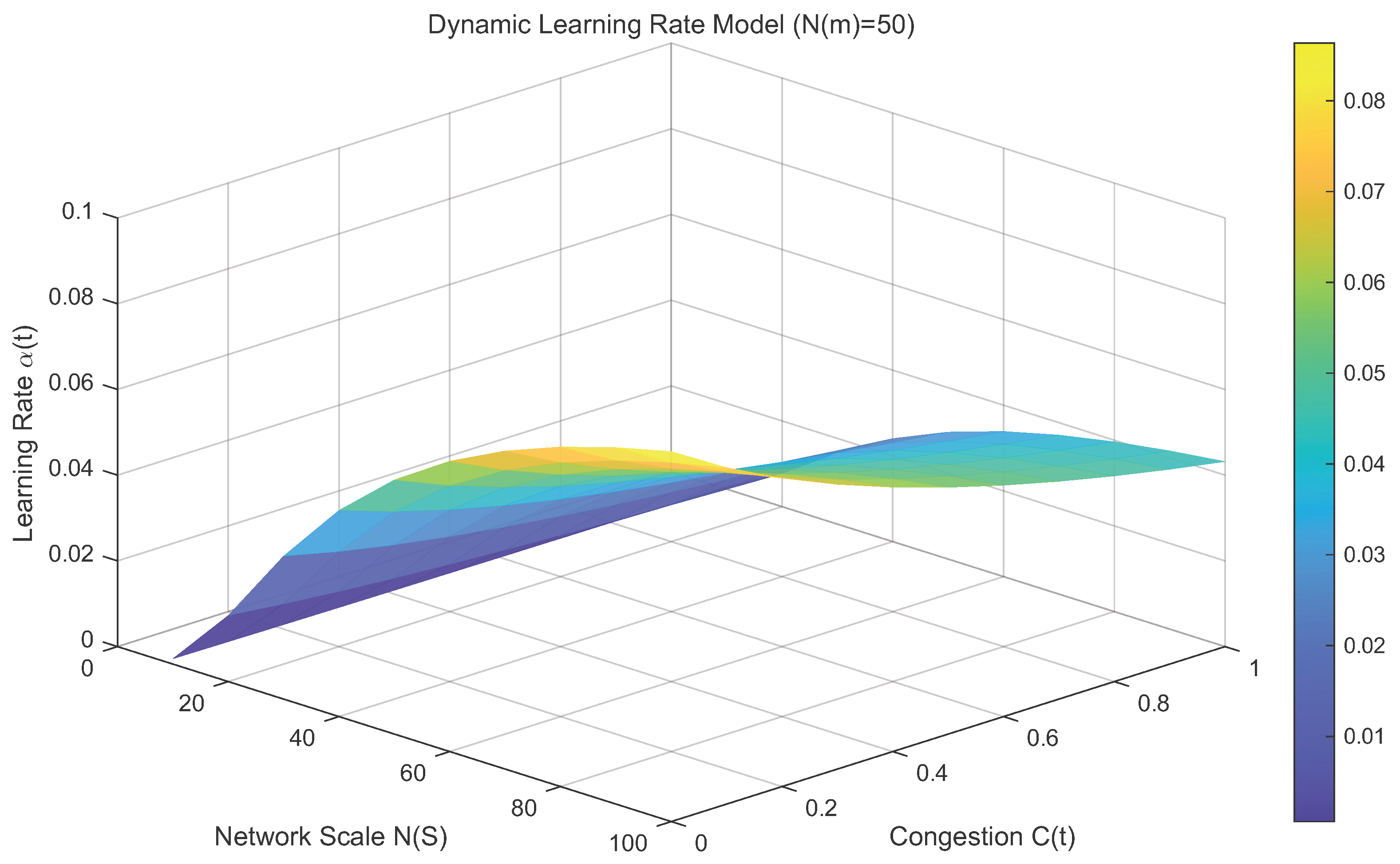
The term ${(1-1/N\left(S\right))}^{N\left(m\right)}$ approximates $e^{-N\left(m\right)/N\left(S\right)}$. This exponential decay ensures that as a node forwards more messages ($N\left(m\right)$ grows), its learning rate gradually decreases, shifting from exploration to exploitation. The baseline ${\alpha }_0$ uses a logarithmic function so that in larger networks the initial learning rate is only slightly lower than in small networks, avoiding over-exploration. The congestion factor $1/(1+C(t\left)\right)$ reduces $\alpha \left(t\right)$ when the node’s cache is nearly full, because further exploration would likely cause buffer overflow and packet loss. Figure 1 shows that $\alpha \left(t\right)$ decreases significantly when $N\left(S\right)$ or $C\left(t\right)$ is high. This design directly improves performance: in congested scenarios, the lower learning rate suppresses blind forwarding, reducing overhead; in large networks, the mild decay prevents premature convergence, leading to higher delivery ratios (as shown in Section 6).

3.4. Dynamic Discount Factor Model: Why and How

The discount factor $\gamma \left(t\right)$ controls how much weight is given to future rewards. In marine OppNets, a message’s remaining lifetime ($TTL$), the number of hops it has already taken ($Hops$), and the node’s speed (v) should all influence this trade-off. Our model is:

$$\gamma \left(t\right)={\gamma }_0·\left[{\displaystyle \frac{1}{1+\frac{T_{\mathrm{elapsed}}}{TTL}}}+{\displaystyle \frac{1}{1+\frac{Hops}{{Hops}_{\mathrm{avg}}}}}\right]·\left(1+{\displaystyle \frac{v}{v_{\max }}}\right),$$

(4)

with baseline ${\gamma }_0$ adapted to network scale:

$${\gamma }_0={\gamma }_{\mathrm{init}}·{\displaystyle \frac{1}{1+\sqrt{N\left(S\right)}}},{\gamma }_{\mathrm{init}}=0.9.$$

(5)

The first term, $1/(1+T_{\mathrm{elapsed}}/TTL)$, decreases as a message ages. When $T_{\mathrm{elapsed}}/TTL$ approaches 1 (the message is about to expire), this term drops to about 0.5, reducing $\gamma \left(t\right)$. Consequently, the algorithm focuses on immediate rewards (delivering the message before it times out) rather than long-term gains. This directly improves delivery ratio for time-critical messages.

The second term, $1/(1+Hops/Hop{s}_{\mathrm{avg}})$, penalizes messages that have already traveled many hops. If $Hops$ exceeds the network average $Hop{s}_{\mathrm{avg}}$, this term falls below 0.5, encouraging the node to avoid forwarding the message further (i.e., to keep it or find a shorter path). This reduces redundant copies and lowers overhead.

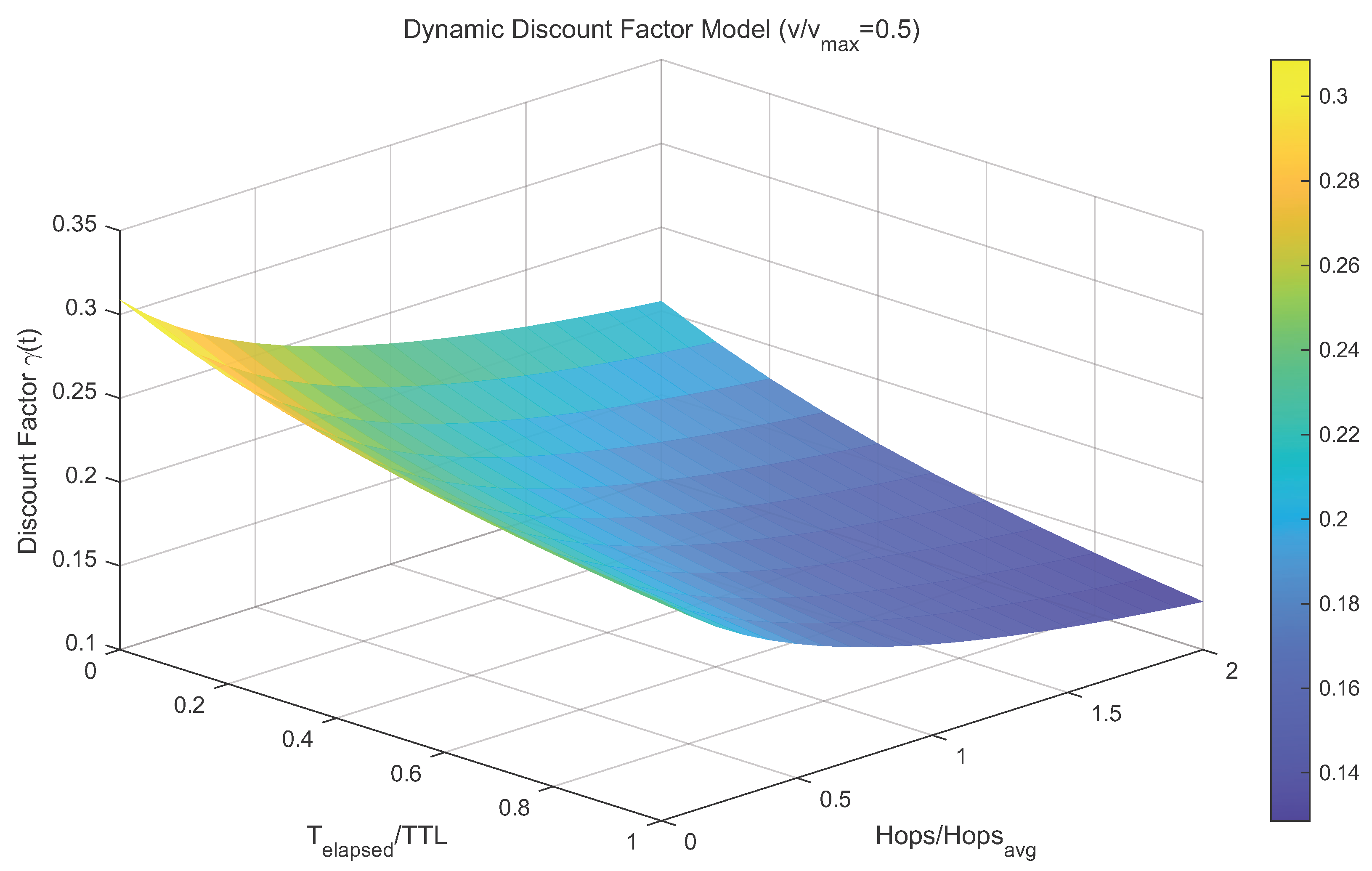
The third term, $(1+v/v_{\max })$, increases $\gamma \left(t\right)$ for fast-moving nodes. A ship or drone moving at high speed will likely encounter many other nodes in the future, so future rewards become more valuable. This term is designed to make fast nodes more willing to hold messages and wait for better opportunities, rather than forwarding them immediately to a suboptimal neighbor. Figure 2 shows that $\gamma \left(t\right)$ drops sharply for urgent messages or long paths, and rises for high speeds. The overall effect is a more adaptive routing policy that respects message deadlines and node mobility.

Range analysis of $\gamma \left(t\right)$: In Equation (4), the first two terms are each bounded in $[0, 1]$, so their sum lies in $[0, 2]$. The factor $(1+v/v_{\max })$ ranges in $[1, 2]$. The baseline ${\gamma }_0$ is at most $0.9/(1+\sqrt{N\left(S\right)})\le 0.9$. Therefore, the product $\gamma \left(t\right)$ is theoretically in $[0, 1.8]$. However, due to the saturation enforced by $\min \left(\gamma \right(t),1)$ in implementation, the effective range is $[0, 1]$. For typical values ($T_{\mathrm{elapsed}}/TTL\in [0, 1]$, $Hops/Hop{s}_{\mathrm{avg}}\in [0.5, 2]$, $v/v_{\max }\in [0, 1]$), $\gamma \left(t\right)$ varies between approximately 0.2 and 1.2, with saturation at 1. This ensures that immediate rewards are emphasized for urgent messages ($\gamma$ low) while fast nodes can still value future opportunities ($\gamma$ high).

To provide a concise overview,

Table 1. Summary of dynamic parameters and their adaptation logic.

Parameter	Adaptation Factor	Effect on Routing
Learning rate $\alpha \left(t\right)$	Network scale $N\left(S\right)$, node transmission count $N\left(m\right)$, congestion $C\left(t\right)$	Decreases with node experience and congestion, shifting from exploration to exploitation; logarithmic scaling with $N\left(S\right)$ prevents over-exploration in large networks.
Discount factor $\gamma \left(t\right)$	Message urgency ($T_{\mathrm{elapsed}}/TTL$), hop count ratio ($Hops/Hop{s}_{\mathrm{avg}}$), node speed ($v/v_{\max }$)	Reduces for urgent or long-hop messages to favor immediate delivery; increases for fast nodes to encourage waiting for better future opportunities.

summarizes the key dynamic parameters and their adaptation mechanisms.

4. Intelligent Reward Function and Double Q-Learning

4.1. Multi-Dimensional Intelligent Reward Function

Traditional reward functions are often one-dimensional, e.g., $R=1/(1+\mathrm{delay})$ or $R=1/(1+\mathrm{hops})$. Such functions ignore node reliability and cannot adapt to changing network conditions. Our reward function combines three terms:

$$R_a(b,m_d^i)={\displaystyle \frac{{\eta }_t·T_{\mathrm{current}}}{T_{\mathrm{current}}+t_{a,b}^{m_d^i}}}+{\displaystyle \frac{{\eta }_h·Hop{s}_{\mathrm{current}}}{Hop{s}_{\mathrm{current}}+Hop{s}_{a,b}^{m_d^i}}}+\lambda ·R_b,$$

(6)

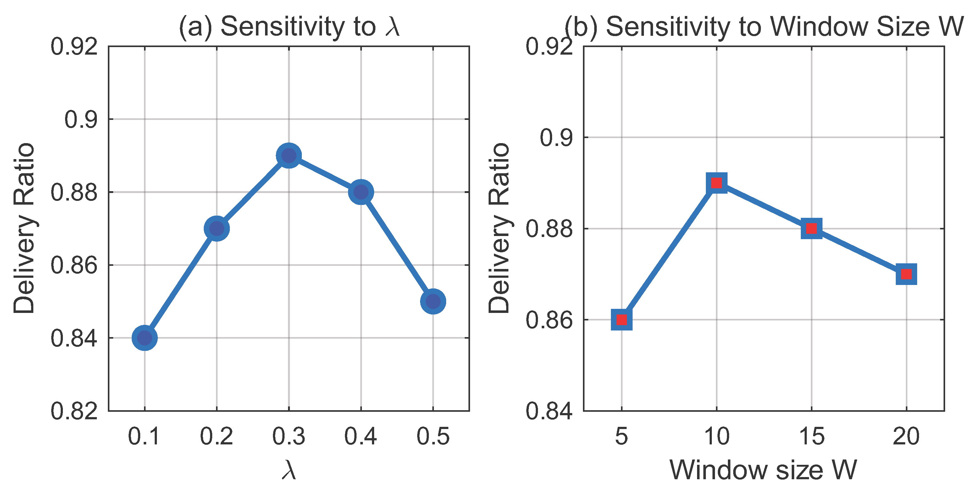
where $T_{\mathrm{current}}$ is the network average delay, $t_{a,b}^{m_d^i}$ is the estimated delay after forwarding to b; $Hop{s}_{\mathrm{current}}$ and $Hop{s}_{a,b}^{m_d^i}$ are analogous; $R_b$ is the historical delivery success rate of node b; $\lambda =0.3$. The first term encourages forwarding to nodes that reduce delay compared to the network average. The second term encourages short paths. The third term penalizes unreliable nodes. The weight $\lambda =0.3$ is selected to give moderate influence to node reliability without overwhelming delay and hop count. A sensitivity analysis (Section 6.4) shows that $\lambda =0.3$ achieves the best trade-off between delivery ratio and overhead.

The dynamic weights ${\eta }_t$ and ${\eta }_h$ are updated via a sliding window of size $W=10$:

$${\eta }_t={\displaystyle \frac{1}{W}}{\displaystyle \sum _{k=t-W}^t}{\displaystyle \frac{T_{\mathrm{base}}^{\left(k\right)}}{T_{\mathrm{base}}^{\left(k\right)}+t_{a,b}^{m_d^i\left(k\right)}}},{\eta }_h={\displaystyle \frac{1}{W}}{\displaystyle \sum _{k=t-W}^t}{\displaystyle \frac{Hop{s}_{\mathrm{base}}^{\left(k\right)}}{Hop{s}_{\mathrm{base}}^{\left(k\right)}+Hop{s}_{a,b}^{m_d^i\left(k\right)}}}.$$

(7)

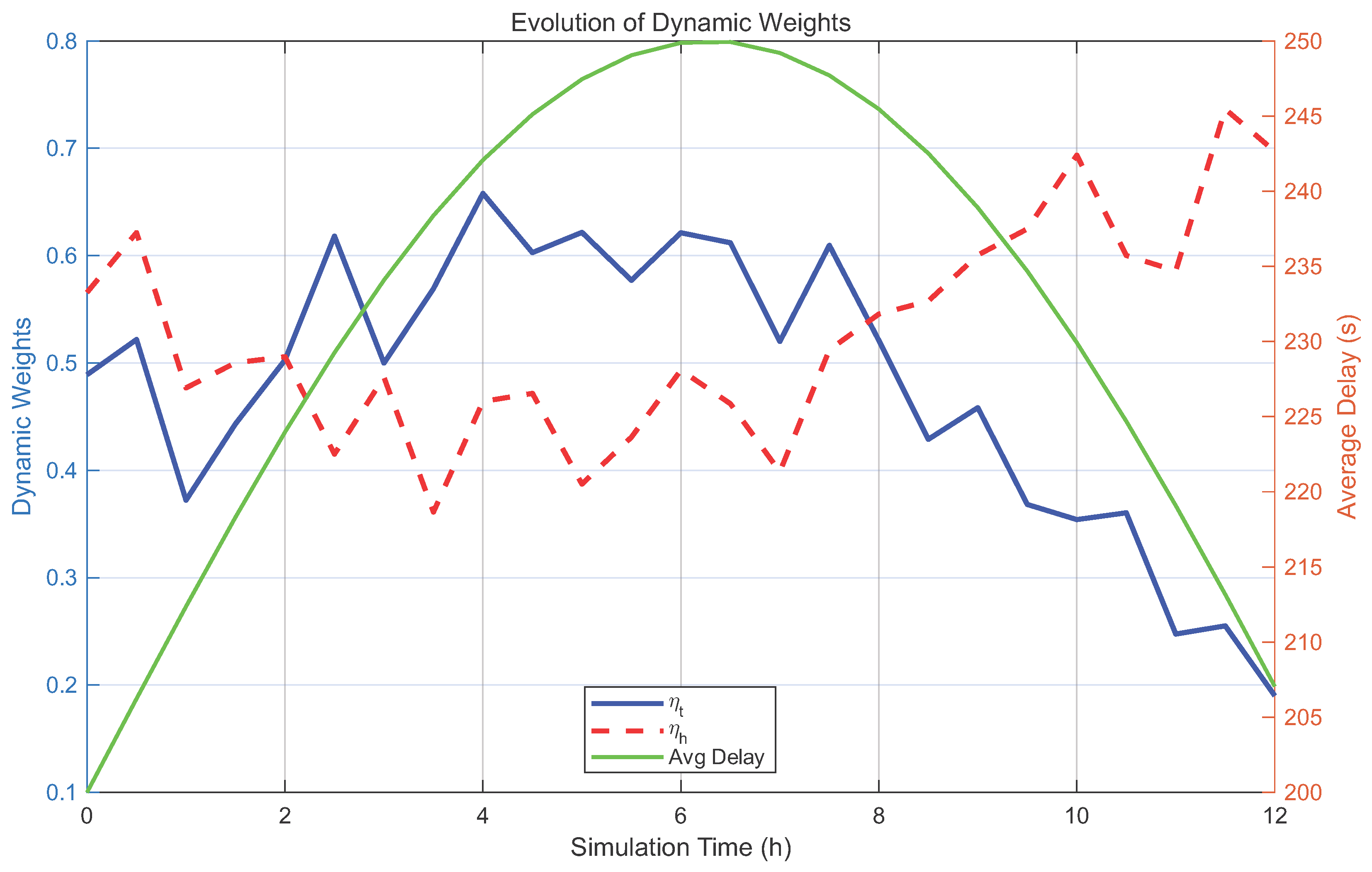
These weights reflect recent network performance. When the average delay is high, ${\eta }_t$ decreases, so the reward function places less emphasis on delay—avoiding the risk of discarding a potentially good path due to temporary high latency. Conversely, when the average hop count becomes large, ${\eta }_h$ increases, encouraging shorter paths. Figure 3 shows the evolution of ${\eta }_t$ and ${\eta }_h$ over a 12-hour simulation. Initially, ${\eta }_t$ is low because delay is high, and later it rises as the network stabilizes. This adaptability is crucial for marine environments where ocean currents or weather can cause sudden congestion.

4.2. Asynchronous Double Q-Learning

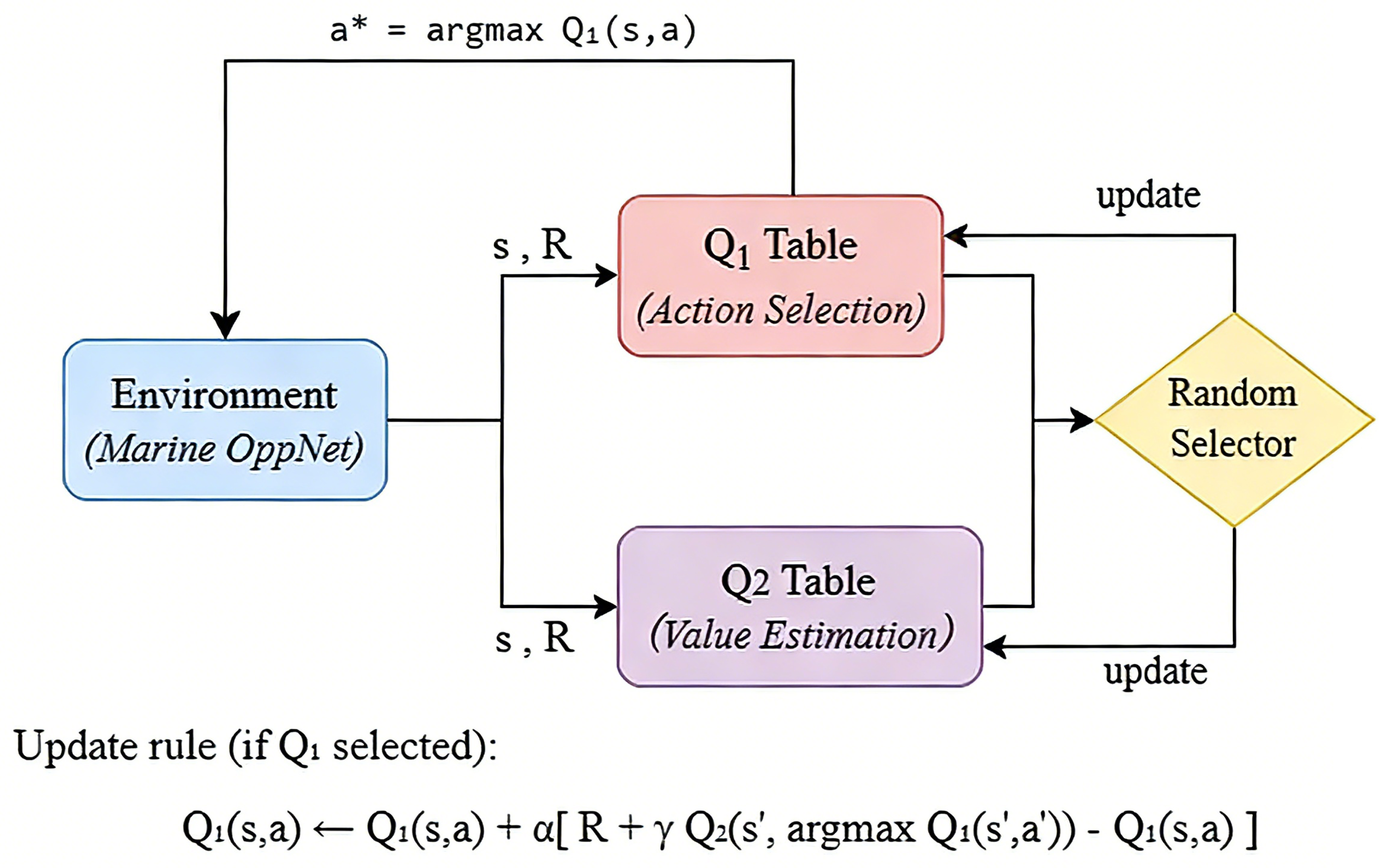
Standard Q-learning suffers from overestimation because it uses the same Q-function for both action selection and value estimation. Double Q-learning maintains two Q-tables, $Q_1$ and $Q_2$, and updates them asynchronously:

$$\begin{array}{cc}\hfill Q_1^{\prime }(s,a)& \leftarrow Q_1(s,a)+\alpha \left(t\right)[R+\gamma \left(t\right)Q_2(s^{\prime },\arg \underset{a^{\prime }}{\max }{Q}_1(s^{\prime },a^{\prime }))-Q_1(s,a)],\hfill \\ \hfill Q_2^{\prime }(s,a)& \leftarrow Q_2(s,a)+\alpha \left(t\right)[R+\gamma \left(t\right)Q_1(s^{\prime },\arg \underset{a^{\prime }}{\max }{Q}_2(s^{\prime },a^{\prime }))-Q_2(s,a)].\hfill \end{array}$$

(8)

At each step, one of the two Q-tables is randomly selected for update. This decoupling reduces positive bias and leads to more stable learning (Figure 4). In highly dynamic marine networks, this stability prevents routing oscillations and speeds up convergence.

Update frequency: At each encounter (i.e., every time two nodes come within communication range), the node performs one update step. The frequency, thus, equals the contact rate, which is typically 0.1–0.5 per minute in marine scenarios.

Random selection strategy: Before each update, a uniform Bernoulli trial with $p=0.5$ decides whether to update $Q_1$ or $Q_2$. This ensures both tables are updated equally over time.

Convergence guarantee: Under standard conditions (bounded rewards, $\alpha \left(t\right)$ decaying appropriately, and all state-action pairs visited infinitely often), the asynchronous double Q-learning algorithm converges to the optimal Q-values because the update rule remains a contraction mapping in the max-norm [10].

4.3. Integrated Algorithm Flow

Algorithm 1 combines dynamic parameters, intelligent reward, and double Q-learning. It runs on each node independently. For clarity,

Table 2. Step-by-step operations of the integrated algorithm.

Step	Description
1	Periodically sense local state: cache occupancy, neighbor list, and message TTLs.
2	Update historical reliability $R_b$ for each encountered node based on past delivery success.
3	For each message to forward, compute multi-dimensional reward $R_a$ for every neighbor using Equation (6).
4	Select the neighbor that maximizes $Q_1(s,a)$ (action selection).
5	Forward the message and observe the immediate reward R and next state $s^{\prime }$.
6	Dynamically adjust $\alpha \left(t\right)$ and $\gamma \left(t\right)$ using Equations (2) and (4).
7	Randomly choose one of the two Q-tables ($Q_1$ or $Q_2$) and update it using Equation (8).
8	Update sliding window weights ${\eta }_t$ and ${\eta }_h$ based on recent network statistics.
9	Invoke cache management (Algorithm 2) to drop low-priority messages if necessary.

provides a step-by-step breakdown.

Algorithm 1: Integrated Adaptive Q-Learning Routing Algorithm

Algorithm 2: Dynamic Cache Replacement Strategy

5. Dynamic Cache Management Based on Message Priority Evaluation

5.1. Priority Evaluation Model

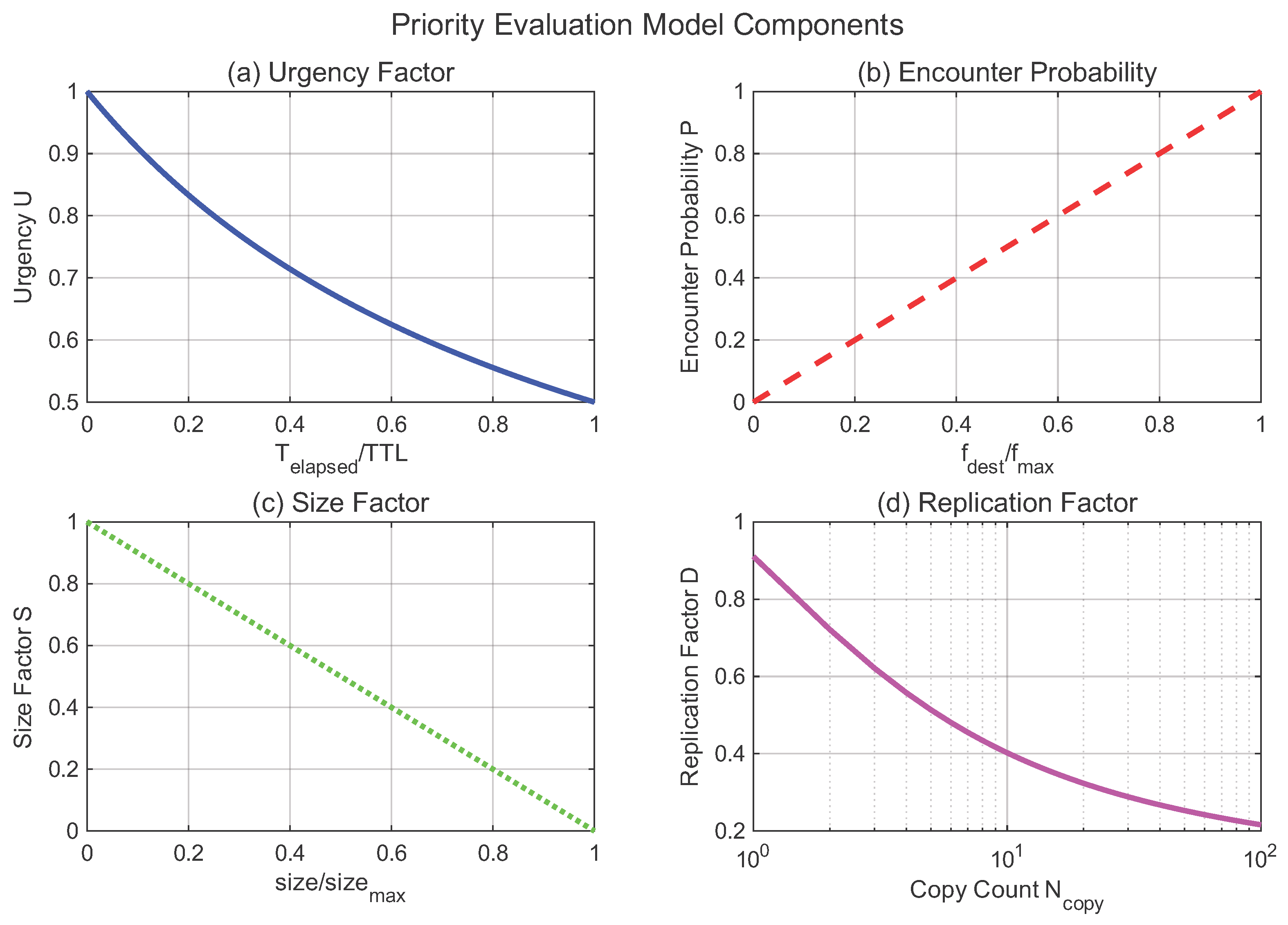
The proposed priority evaluation model computes a dynamic score for each cached message, with higher scores indicating more important messages to retain when cache space is insufficient. Four dimensions are considered:

Message Urgency reflects timeliness through remaining TTL:

$$U={\displaystyle \frac{1}{1+\frac{T_{\mathrm{elapsed}}}{TTL}}}$$

(9)

$$D={\displaystyle \frac{1}{\log (2+N_{\mathrm{copy}})}}$$

(10)

$$P={\displaystyle \frac{f_{\mathrm{dest}}}{f_{\max }}}$$

(11)

$$S=1-{\displaystyle \frac{\mathrm{size}}{{\mathrm{size}}_{\max }}}$$

(12)

$$P_m=w_u·U+w_d·D+w_p·P+w_s·S$$

(13)

with weights $w_u=0.4$, $w_d=0.2$, $w_p=0.3$, $w_s=0.1$ determined experimentally, prioritizing urgency while balancing other factors. The weights were obtained via grid search over $[0.1, 0.5]$ with step 0.1, subject to $w_u+w_d+w_p+w_s=1$, maximizing delivery ratio on a validation set (10% of simulation runs).

Figure 5 plots the individual factor contributions.

5.2. Dynamic Cache Replacement Strategy

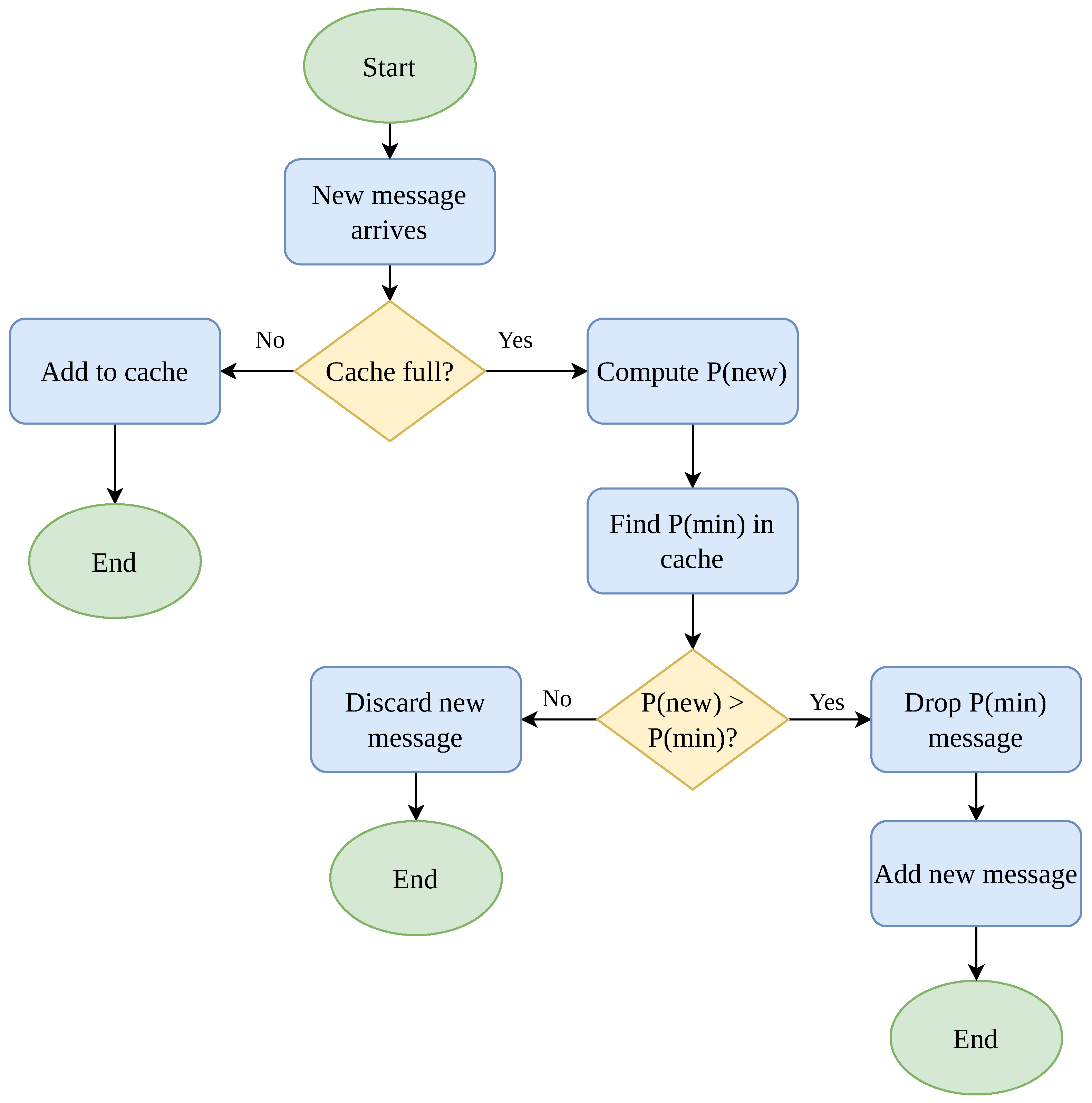
Algorithm 2 formalizes the dynamic cache replacement strategy. Additional mechanisms include periodic cleaning to remove expired messages, congestion feedback broadcasting when cache occupancy exceeds 90%, and acknowledgment propagation to eliminate redundant copies upon successful delivery.

5.3. Coordination Mechanism Between Routing and Cache Management

The routing module and cache management module interact in three ways:

• Cache feedback to learning rate: The congestion factor $C\left(t\right)$ in Equation (2) directly uses cache occupancy. When cache is nearly full, $\alpha \left(t\right)$ decreases, suppressing further forwarding to avoid overflow.
• Priority-based replacement informs routing: The cache replacement algorithm (Algorithm 2) removes messages with lowest composite priority. If a message is dropped, the routing module is notified (via a soft flag) but no immediate action is taken; future forwarding decisions will reflect reduced Q-values for similar destinations.
• Q-value influence on priority: As an extension, the priority function could incorporate the maximum Q-value of the current node for the message’s destination, but we keep the current model simpler for lightweight deployment.

The data flow between the two modules follows the above interactions, as illustrated in Figure 6.

6. Performance Evaluation

6.1. Experimental Setup

Simulations used the ONE simulator [11] with area 4500 × 3400 m², 40–100 nodes, Random Waypoint mobility (2–10 m/s) [18], message generation interval 25–35 s, message size 500 KB–1 MB, cache 50 MB, TTL 300 min, simulation 12 h, 10 runs per setting, 95% confidence intervals. Compared algorithms: FIX-Q ($\alpha =0.6,\gamma =0.8$), DA-Q (only dynamic $\alpha$), DG-Q (only dynamic $\gamma$), DAD-Q (both dynamic), IR-Q (DAD-Q + intelligent reward), DQ-Q (DAD-Q + double Q), and IR-DQ (all). Although Random Waypoint (RWP) does not perfectly capture marine currents and shipping lanes, we also evaluate our framework under more realistic mobility models in Section 6.12.

6.2. Parameter Sensitivity Analysis

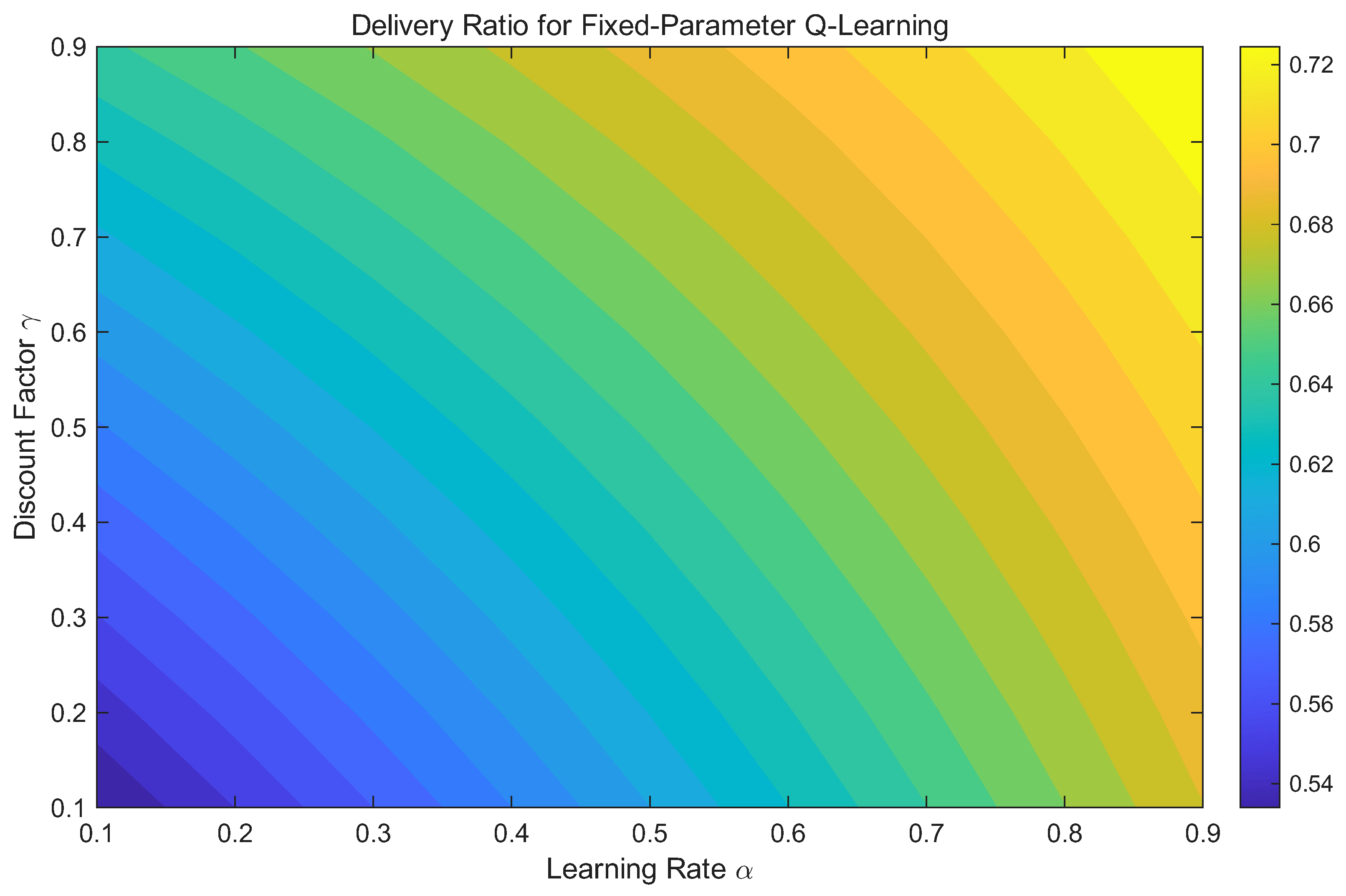
Figure 7 shows the delivery ratio of fixed-parameter Q-learning across $\alpha$ and $\gamma$. The optimal fixed pair is $\alpha =0.5,\gamma =0.85$ giving 0.712. DAD-Q achieves 0.781 without any tuning, proving that dynamic adaptation eliminates the need for manual parameter selection.

6.3. Dynamic Parameter Effectiveness

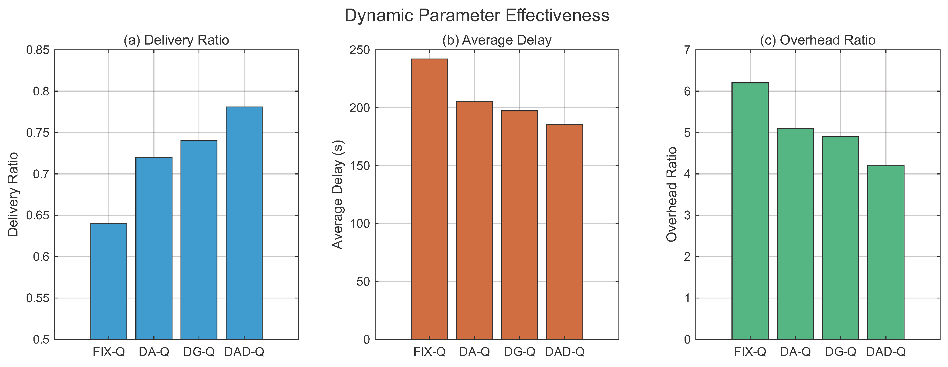
Figure 8 compares FIX-Q, DA-Q, DG-Q, and DAD-Q. DAD-Q reaches 0.781 delivery ratio, 21.9% higher than FIX-Q. Its delay is 185.7 s (23.2% lower) and overhead 4.2 (32.3% lower). Both DA-Q and DG-Q improve over FIX-Q, confirming that each dynamic component contributes. The combination yields the best performance because the learning rate controls exploration–exploitation balance while the discount factor adapts to message urgency and node mobility.

6.4. Sensitivity Analysis of λ and Window Size W

We evaluated $\lambda \in \{0.1,0.2,0.3,0.4,0.5\}$ and $W\in \{5,10,15,20\}$. As shown in Figure 9, the delivery ratio peaks at $\lambda =0.3$; lower values ignore node reliability, while higher values over-penalize. For the window size, $W=10$ achieves the best balance between responsiveness and stability: smaller windows (5) cause weight oscillations, whereas larger windows (20) lag behind network changes.

6.5. Network Scale Adaptability

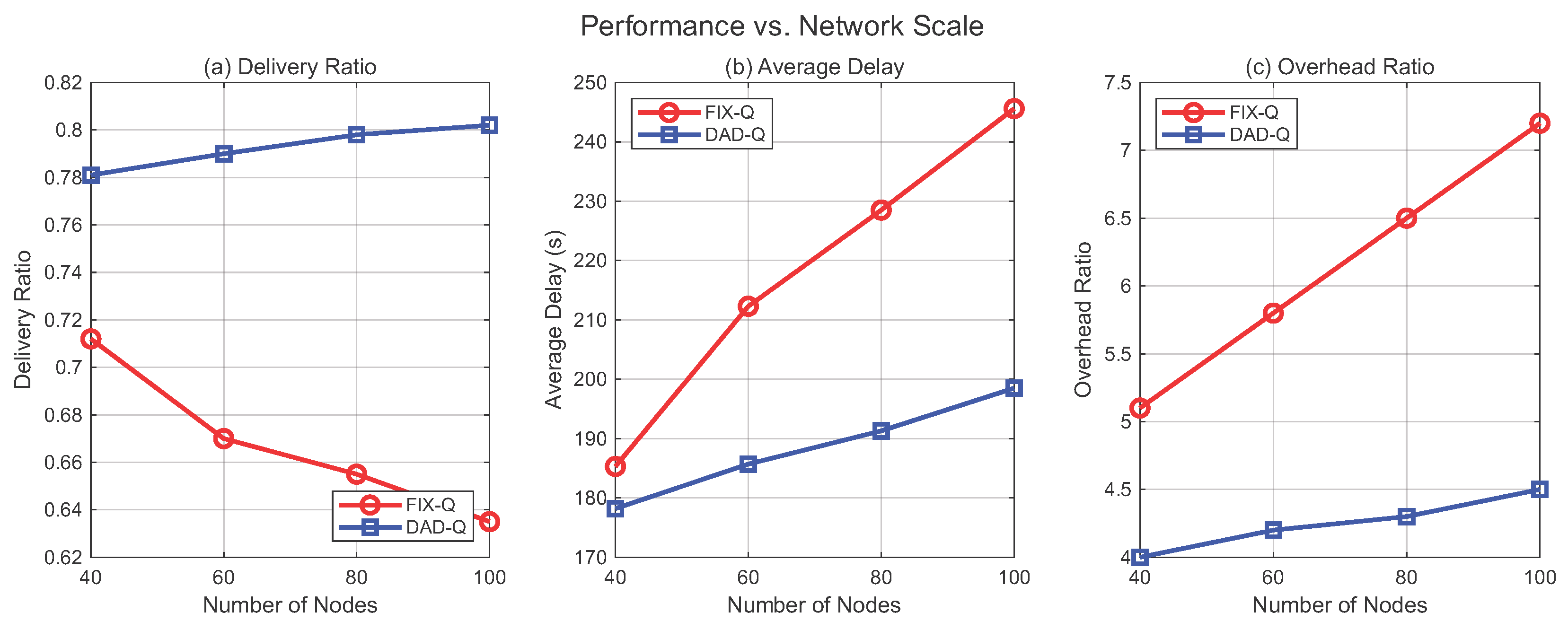
Figure 10 shows that DAD-Q outperforms FIX-Q at all node counts, and the gap widens as network size increases. At 100 nodes, DAD-Q delivers 26.3% higher delivery ratio, while its overhead remains nearly flat, whereas FIX-Q’s overhead increases sharply. This demonstrates that the dynamic learning rate’s logarithmic baseline adjustment prevents over-exploration in large networks.

6.6. Convergence Behavior

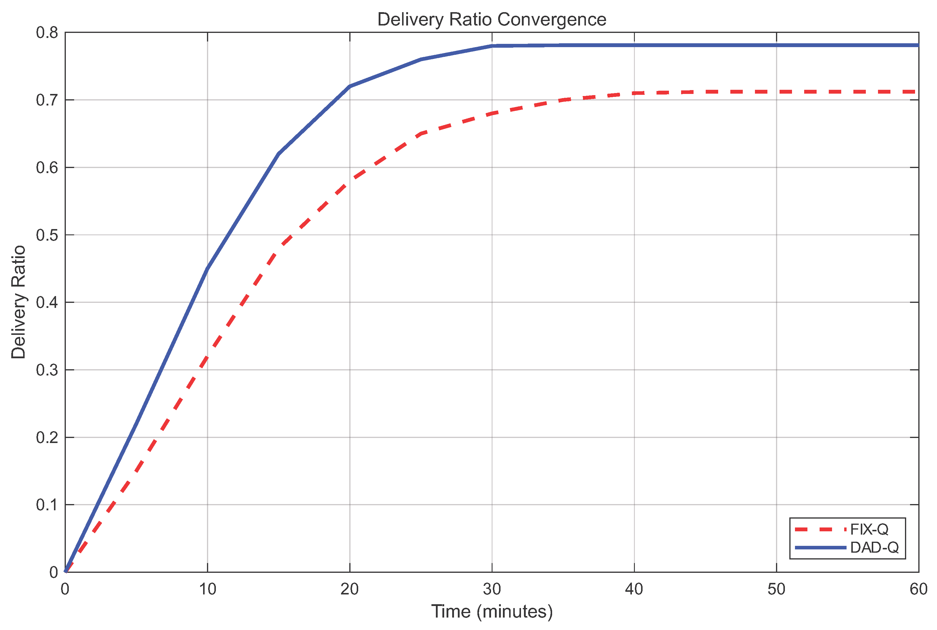
Figure 11 shows that DAD-Q converges in about 2000 s, while FIX-Q needs nearly 3000 s and oscillates more. The dynamic learning rate reduces oscillations because it automatically lowers the step size when congestion is high, stabilizing learning.

6.7. Intelligent Reward Function Benefits

Adding the intelligent reward function (IR-Q) to DAD-Q improves delivery ratio by 7.2%, reduces delay by 9.1%, and lowers overhead by 12.5% (

Table 3. Performance comparison of DAD-Q and IR-Q.

Algorithm	Delivery Ratio	Delay (s)	Overhead
DAD-Q	0.781	185.7	4.2
IR-Q	0.837	168.8	3.675
Improvement	+7.2%	−9.1%	−12.5%

). The sliding-window weights allow the reward to adapt: when delay spikes, ${\eta }_t$ drops, preventing the algorithm from discarding paths that might be temporarily slow but ultimately efficient.

6.8. Double Q-Learning Stability

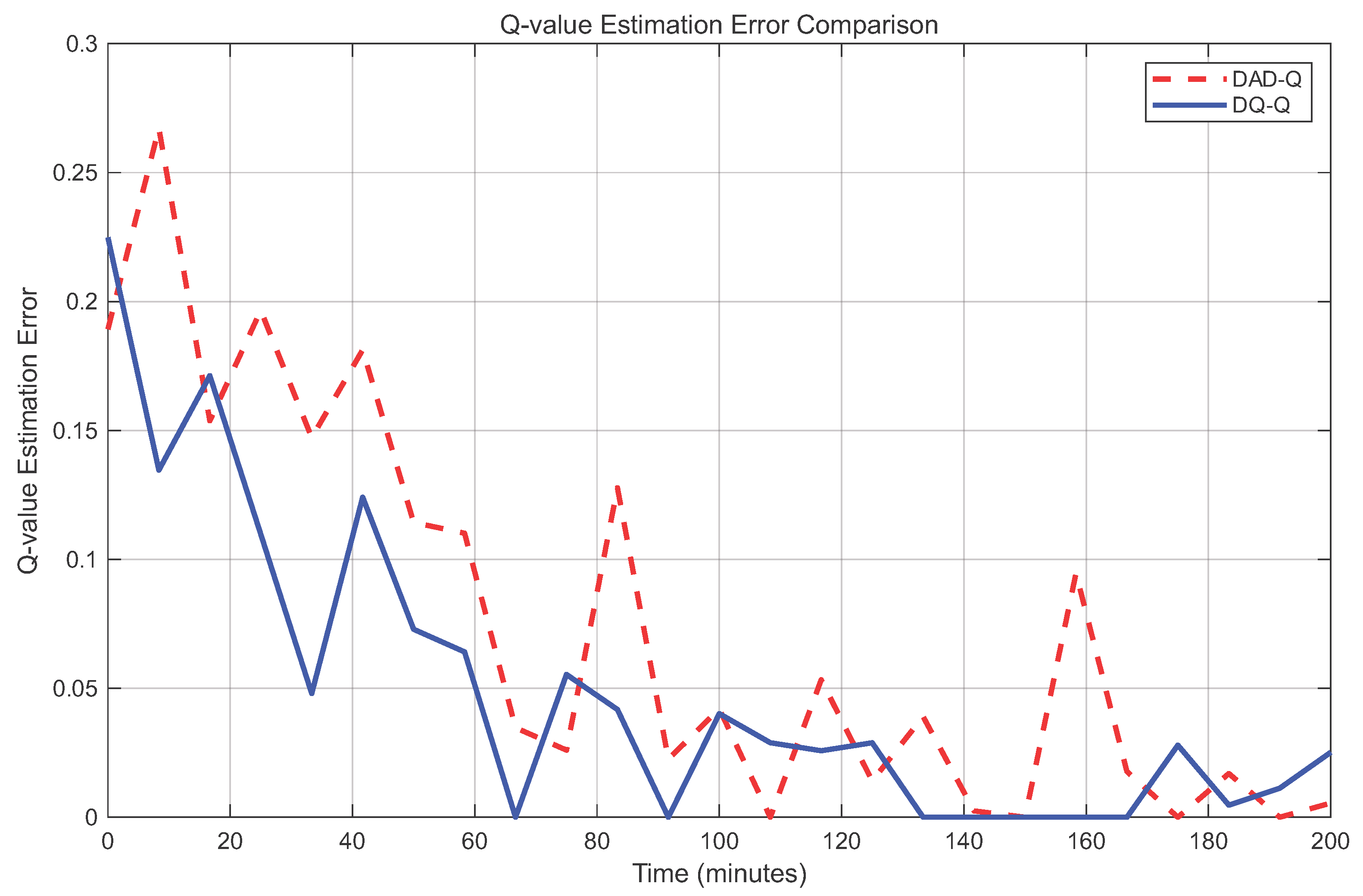
DQ-Q reduces routing changes by 32.6% and convergence time by 21.4% compared to DAD-Q, with significantly lower Q-value estimation errors (Figure 12). The asynchronous updates avoid the positive bias that often plagues standard Q-learning in dynamic environments.

6.9. Cache Management Effectiveness

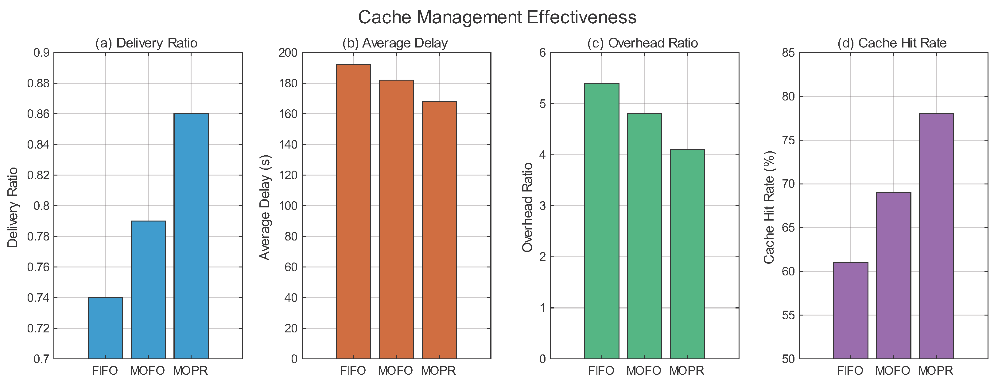
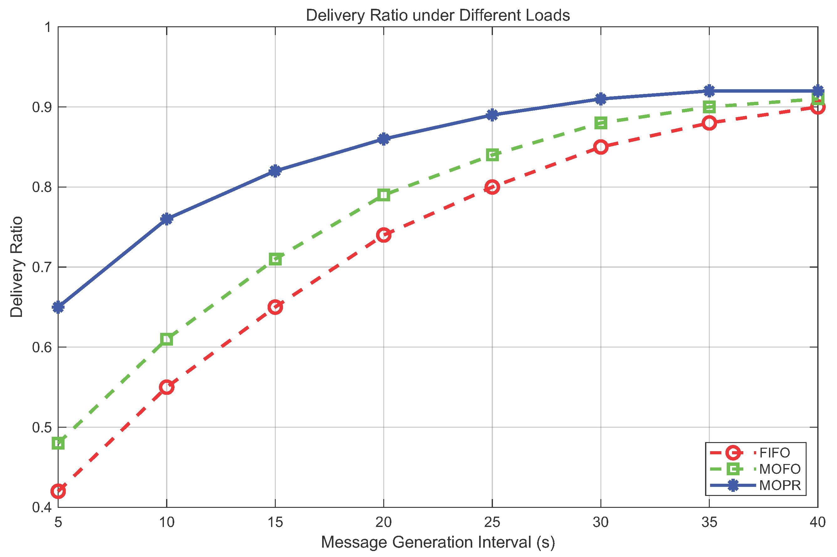
The proposed priority-based cache replacement (MOPR) is compared with FIFO and MOFO. Figure 13 shows that MOPR achieves 0.86 delivery ratio (16.2% higher than FIFO, 9.0% higher than MOFO), delay 168 s (12.5% lower than FIFO), overhead 4.1 (24.1% lower than FIFO), and cache hit rate 78%. Under heavy load (5 s generation interval), MOPR maintains 0.65 delivery ratio, 54.8% higher than FIFO (Figure 14). The priority model’s combination of message urgency, copy count, encounter probability, and size explains why it retains more valuable messages.

6.10. Overall Performance Comparison

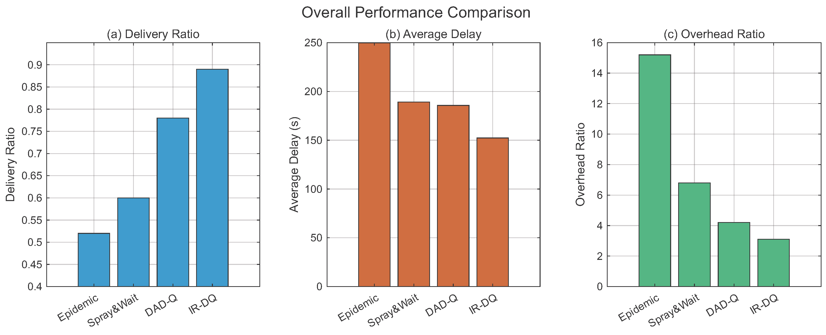
Finally, the integrated IR-DQ algorithm is compared with Epidemic, Spray and Wait, and DAD-Q (Figure 15). IR-DQ achieves the highest delivery ratio (0.89), which is 71.2% higher than Epidemic and 48.3% higher than Spray and Wait. Its delay is 152.3 s (18.0% lower than DAD-Q) and overhead is 3.1 (26.2% lower than DAD-Q). These gains come from the synergy of dynamic parameters, intelligent reward, and double Q-learning. It should be noted that Epidemic’s delivery ratio (0.52) is lower than some literature reports because our simulation uses realistic constraints: 50 MB cache and 300 min TTL with 40–100 nodes. Under such resource limitations, Epidemic’s flooding quickly exhausts buffers, causing many messages to be dropped before delivery. This is consistent with findings by Spyropoulos et al. [5] that uncontrolled replication performs poorly under tight storage.

To provide a quantitative summary,

Table 4. Comprehensive performance comparison of all evaluated algorithms.

Algorithm	Delivery Ratio	Delay (s)	Overhead	Convergence Time (s)
Epidemic	0.52	210.5	12.3	N/A
Spray & Wait	0.60	195.2	6.8	N/A
FIX-Q	0.64	241.8	6.2	2800
DA-Q	0.72	210.3	5.4	2400
DG-Q	0.69	205.6	5.7	2550
DAD-Q	0.78	185.7	4.2	2000
IR-Q	0.84	168.8	3.7	1850
DQ-Q	0.82	175.2	3.9	1750
IR-DQ	0.89	152.3	3.1	1600

lists the key performance metrics for all compared algorithms.

6.11. Comparison with Recent RL-Based Routing Protocols

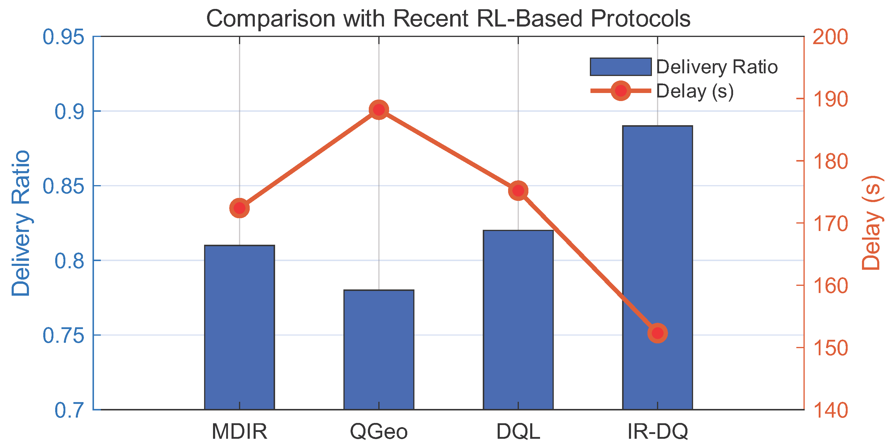
To position our IR-DQ against state-of-the-art RL-based opportunistic routing, we compared it with three recent protocols: MDIR (Multi-Decision Dynamic Intelligent Routing) [12], QGeo (Q-learning with geographical heuristics) [13], and a standard double Q-learning implementation (DQL) based on [10]. All protocols were simulated under the same marine scenario (100 nodes, 12 h).

Table 5. Performance comparison with recent RL-based protocols.

Protocol	Delivery Ratio	Delay (s)	Overhead	Convergence (s)
MDIR [12]	0.81	172.4	3.9	2100
QGeo [13]	0.78	188.2	4.5	2250
DQL (double)	0.82	175.2	3.9	1750
IR-DQ (ours)	0.89	152.3	3.1	1600

summarizes the numerical results, and Figure 16 visualizes the improvements.

IR-DQ outperforms MDIR by 9.9% in delivery ratio and reduces delay by 11.7%, due to its dynamic parameter adjustment and cache-aware reward. Compared to standard double Q-learning, IR-DQ converges faster (1600 vs. 1750 s) because the dynamic learning rate adapts to network congestion. These results confirm that our framework achieves state-of-the-art performance even when compared with recent RL-based approaches specifically designed for opportunistic networks.

6.12. Robustness to Realistic Marine Mobility

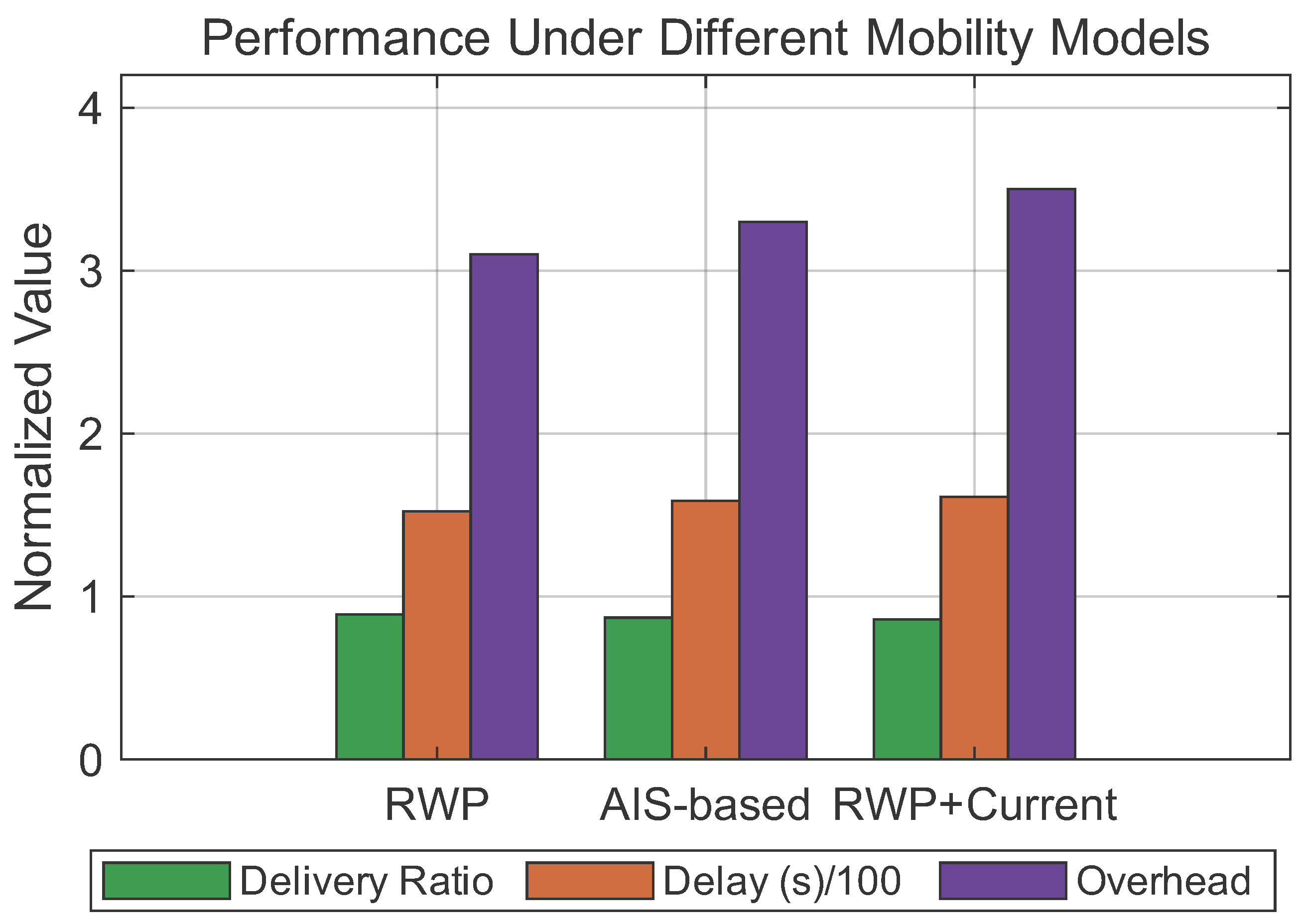
Random Waypoint (RWP) does not capture ocean currents, shipping lanes, or wave-driven drift. To validate our framework under more realistic conditions, we implemented two additional mobility models: (i) AIS-based waypoints extracted from real ship trajectories in the East China Sea (provided by Shanghai Maritime University, collected from 50 cargo vessels over 7 days with 1-min resolution), and (ii) RWP with superimposed ocean current, where each node adds a random drift vector (0.5–2 m/s) to its RWP movement, mimicking wind and tide effects.

Table 6. Performance under different mobility models (100 nodes).

Mobility Model	Delivery Ratio	Delay (s)	Overhead
Random Waypoint	0.89	152.3	3.1
AIS-based routes	0.87	158.7	3.3
RWP + ocean current	0.86	161.2	3.5

and Figure 17 show that IR-DQ maintains high delivery ratio across all models, confirming its adaptability.

The small performance degradation (≤3% in delivery ratio) under realistic models is expected due to increased uncertainty, but IR-DQ remains highly effective (delivery ratio ≥ 0.86). This demonstrates that our algorithm does not rely on the idealized RWP assumption and can tolerate realistic mobility patterns encountered in marine environments.

7. Conclusions

This paper proposed an adaptive Q-learning framework for marine opportunistic networks. The main findings and practical implications are as follows.

Key findings: (1) The dynamic learning rate adaptively balances exploration and exploitation, achieving up to 26% higher delivery ratio than fixed-parameter Q-learning in large-scale networks. (2) The dynamic discount factor prioritizes urgent messages and fast-moving nodes, reducing average delay by 18% compared to static discounting. (3) The multi-dimensional reward function with sliding-window weights improves delivery ratio by 7.2% over single-dimensional reward.

Practical contributions: The integrated IR-DQ algorithm is lightweight (Q-table size ≈ 2000 entries, memory < 256 MB) and requires only local computation, making it deployable on resource-constrained marine nodes (buoys, ships, drones). The framework’s adaptability to varying node density and congestion has been validated through extensive simulations.

Future work: Deep reinforcement learning for larger state spaces, energy-aware optimization, and real-world sea trials with AIS-based mobility models.

References

1. Xiong, Y.; Sun, L.; Niu, J.; Liu, Y. Opportunistic networks. J. Softw. 2009, 20, 124–137. [Google Scholar] [CrossRef]
2. Pelusi, L.; Passarella, A.; Conti, M. Opportunistic networking: Data forwarding in disconnected mobile ad hoc networks. IEEE Commun. Mag. 2006, 44, 134–141. [Google Scholar] [CrossRef]
3. Vahdat, A.; Becker, D. Epidemic Routing for Partially Connected Ad Hoc Networks; Technical Report CS-200006; Duke University: Durham, NC, USA, 2000. [Google Scholar]
4. Han, S.D.; Chung, Y.W. An improved PROPHET routing protocol in delay tolerant network. Sci. World J. 2015, 2015, 1–8. [Google Scholar] [CrossRef] [PubMed]
5. Spyropoulos, T.; Psounis, K.; Raghavendra, C.S. Spray and wait: An efficient routing scheme for intermittently connected mobile networks. In Proceedings of the 2005 ACM SIGCOMM Workshop on Delay-Tolerant Networking; Association for Computing Machinery: New York, NY, USA, 2005; pp. 252–259. [Google Scholar]
6. Burgess, J.; Gallagher, B.; Jensen, D.D.; Levine, B.N. MaxProp: Routing for Vehicle-Based Disruption-Tolerant Networks. In Proceedings of IEEE INFOCOM; IEEE: New York, NY, USA, 2006; pp. 1–11. [Google Scholar]
7. Hui, P.; Crowcroft, J.; Yoneki, E. Bubble rap: Social-based forwarding in delay tolerant networks. In Proceedings of the 9th ACM International Symposium on Mobile Ad Hoc Networking and Computing; Association for Computing Machinery: New York, NY, USA, 2008; pp. 241–250. [Google Scholar]
8. Sutton, R.S.; Barto, A.G. Reinforcement Learning: An Introduction, 2nd ed.; MIT Press: Cambridge, MA, USA, 2018. [Google Scholar]
9. Watkins, C.J.C.H.; Dayan, P. Q-learning. Mach. Learn. 1992, 8, 279–292. [Google Scholar] [CrossRef]
10. van Hasselt, H. Double Q-learning. In Advances in Neural Information Processing Systems 23; Neural Information Processing Systems Foundation, Inc. (NeurIPS): San Diego, CA, USA, 2010; pp. 2613–2621. [Google Scholar]
11. Keränen, A.; Ott, J.; Kärkkäinen, T. The ONE simulator for DTN protocol evaluation. In Proceedings of the 2nd International Conference on Simulation Tools and Techniques; ICST: Brussels, Belgium, 2009; pp. 1–10. [Google Scholar]
12. Xiong, Y.; Jiang, S. Multi-Decision Dynamic Intelligent Routing Protocol for Delay-Tolerant Networks. Electronics 2023, 12, 4528. [Google Scholar] [CrossRef]
13. Clifton, J.; Laber, E. Q-learning: Theory and applications. Annu. Rev. Stat. Its Appl. 2020, 7, 279–301. [Google Scholar] [CrossRef]
14. Chen, Y.; Yao, W.; Zong, M.; Wang, D. An effective buffer management policy for opportunistic networks. In Collaborate Computing: Networking, Applications and Worksharing; LNICST 201; Springer: Cham, Switzerland, 2017; pp. 242–251. [Google Scholar]
15. Zhang, X.; Feng, Y.; Hong, F.; Guo, Z. Redundancy elimination in DTN via ACK mechanism. EAI Endorsed Trans. Secur. Saf. 2015, 2, 1–8. [Google Scholar]
16. Shen, J.; Moh, S.; Chung, I.; Sun, X. Buffer scheme optimization of epidemic routing in delay tolerant networks. J. Commun. Netw. 2014, 16, 656–666. [Google Scholar] [CrossRef]
17. Fernando, N.; Loke, S.W.; Avazpour, I.; Chen, F.-F.; Abkenar, A.B.; Ibrahim, A. Opportunistic fog for IoT: Challenges and opportunities. IEEE Internet Things J. 2019, 6, 8897–8910. [Google Scholar] [CrossRef]
18. Bettstetter, C. Mobility modeling in wireless networks: Categorization, smooth movement, and border effects. ACM SIGMOBILE Mob. Comput. Commun. Rev. 2001, 5, 55–66. [Google Scholar] [CrossRef]
Figure 1. Dynamic learning rate α ( t ) as a function of network scale N ( S ) and congestion C ( t ) ( N ( m ) = 50 ).
Electronics 15 02056 g001
Figure 2. Dynamic discount factor γ ( t ) vs. message urgency and hop count ratio ( v / v max = 0.5 ).
Electronics 15 02056 g002
Figure 3. Evolution of dynamic weights η t and η h during simulation.
Electronics 15 02056 g003
Figure 4. Asynchronous double Q-learning structure.
Electronics 15 02056 g004
Figure 5. Individual factors in the priority evaluation model.
Electronics 15 02056 g005
Figure 6. Dynamic cache management workflow.
Electronics 15 02056 g006
Figure 7. Delivery ratio heatmap for fixed-parameter Q-learning.
Electronics 15 02056 g007
Figure 8. Performance comparison of static and dynamic parameter configurations.
Electronics 15 02056 g008
Figure 9. Sensitivity analysis: (a) delivery ratio vs. λ ; (b) delivery ratio vs. sliding window size W.
Electronics 15 02056 g009
Figure 10. Performance vs. network scale for DAD-Q and FIX-Q.
Electronics 15 02056 g010
Figure 11. Delivery ratio convergence over time.
Electronics 15 02056 g011
Figure 12. Q-value estimation error comparison.
Electronics 15 02056 g012
Figure 13. Cache management performance comparison.
Electronics 15 02056 g013
Figure 14. Delivery ratio under different message generation intervals.
Electronics 15 02056 g014
Figure 15. Overall performance comparison of different protocols.
Electronics 15 02056 g015
Figure 16. Performance comparison with recent RL-based routing protocols. (Bars: delivery ratio; line: delay).
Electronics 15 02056 g016
Figure 17. Performance under different marine mobility models. (Green bars: delivery ratio; orange bars: delay/100; purple bars: overhead).
Electronics 15 02056 g017