A DeepWalk Graph Embedding-Enhanced Extreme Learning Machine Method for Online Gearbox Fault Diagnosis

Abstract

Deep learning has become a popular topic among scholars and has attracted widespread attention. However, deep learning methods typically require large datasets to determine model parameters and can only process data in batches. To address the challenges of deep learning models, which rely on batch data and struggle to adapt to industrial streaming data scenarios in gearbox fault diagnosis, this study proposes an online gearbox fault diagnosis method based on a DeepWalk graph embedding-enhanced extreme learning machine (ELM) approach. The method constructs a graph structure in real time for each newly collected vibration signal, uses DeepWalk for unsupervised embedding learning, and extracts low-dimensional features with strong discriminative power. These features are then input into the ELM classifier to achieve adaptive fault type recognition and online incremental model updates. This method does not require historical data to be retrained, thus effectively overcoming the bottleneck of batch retraining and significantly improving diagnostic efficiency and resource utilization. The experimental results show that, under various operating conditions, the proposed method achieves fast and accurate diagnosis of multiple gearbox fault types, with an average accuracy consistently above 95%, thereby demonstrating excellent engineering applicability and real-time performance.

1. Introduction

Rotating machinery is an indispensable component of modern industrial equipment, being widely used in applications such as wind turbines, water pumps, gas turbines, and automotive gearboxes [1]. As the core component of power transmission in rotating machinery, the gearbox’s condition directly impacts the safety and reliability of the entire system. However, due to prolonged operation under variable loads and high-speed conditions, gearboxes are highly susceptible to faults, which can lead to unplanned shutdowns and result in significant economic losses [2]. Therefore, the timely diagnosis of gearbox health is crucial for predictive maintenance and ensuring continuous industrial production [3].

In recent years, with the development of artificial intelligence and big data mining technologies, intelligent diagnostic methods, particularly neural networks, have attracted widespread attention in fault recognition. These methods achieve end-to-end feature learning through multiple layers of nonlinear processing, automatically extracting complex hierarchical features from raw data [4]. Some major neural network families include convolutional neural networks (CNNs), Recurrent Neural Networks (RNNs), Graph Neural Networks (GNNs), and Long Short-Term Memory networks (LSTM), all of which have shown significant results in rotating machinery fault diagnosis [5,6,7,8,9,10]. For example, Jiao et al. [11] proposed a novel integrated framework based on a simplified graph wavelet neural network for planetary gearbox fault diagnosis, achieving high accuracy and robustness. Wang et al. [12] introduced a gearbox fault diagnosis method based on a structure-reparametrized convolutional neural network in edge computing scenarios to address time delays and information loss in the fault diagnosis of industrial cloud applications. To improve fault recognition accuracy, a method based on Graph Neural Networks and Markov Random Fields was proposed [13], which captures key fault information by considering the temporal correlation in signals. To address non-stationary operating conditions, Chen et al. [14] designed an automatic speed-adaptive neural network model for planetary gearbox fault diagnosis.

Nevertheless, current intelligent diagnostic methods are hindered by three core data-centric issues. The first is vibration data scarcity and poor quality: high-quality labeled fault data is expensive to collect industrially, resulting in incomplete, noisy datasets that undermine real-scene performance [15]. The second is weak cross-condition generalization: models trained on fixed conditions (e.g., constant speed) fail to adapt to condition variations, limiting their full-life-cycle applicability [16,17]. The third issue is severe class imbalance: normal samples far outnumber fault ones, thus biasing models and reducing rare fault recognition—these are often accident triggers [18]. Sehri et al. [19] address these gaps via the VibNet framework, which is a large-scale vibration dataset analogous to ImageNet. By fusing multi-source bearing data and leveraging transfer learning, VibNet boosts model generalization, especially for imbalanced data. This highlights that existing methods over-rely on small lab datasets, emphasizing the need for online methods adaptive to industrial data complexity, which aligns with our research goal.

Although existing research has demonstrated strong potential in gearbox fault diagnosis, it typically relies on batch training with data, thus making it difficult to apply directly to streaming data in online monitoring scenarios [20,21,22]. Furthermore, as equipment operates over time, its performance may degrade or exhibit new fault patterns, leading to a significant decline in the diagnostic performance of static models. To address the limitations of existing methods in streaming data monitoring, this study presents the DWELM method, which offers three key contributions: First, it enables the real-time graph-structured modeling of vibration signals through the dynamic construction of k-nearest neighbor (k-NN) graphs, thus overcoming the constraints of traditional approaches such as CNNs and RNNs that depend on fixed inputs and batch-wise training [23]. Second, it integrates unsupervised DeepWalk graph embedding with the fast classification capability of extreme learning machines (ELMs), thus achieving adaptive fault identification in scenarios with scarce annotations [24]. Finally, it introduces a genuine online incremental learning mechanism that only requires the fine-tuning of new nodes and their local neighborhoods without retraining on historical data, thereby substantially improving the adaptability and resource efficiency of industrial real-time monitoring [25]. While extreme learning machines (ELMs) have shown potential for online applications due to their fast training speed, standard ELMs still require new data to be merged with historical data for batch training, thus making true incremental updates unattainable [26,27]. Therefore, this study proposes an online gearbox fault diagnosis method based on a DeepWalk graph embedding-enhanced extreme learning machine (DWELM). The DeepWalk model can adaptively extract features and process continuous data streams in real time, avoiding computational resource waste caused by retraining already processed data, thereby improving model training efficiency and speed. To verify the effectiveness of feature extraction using the DeepWalk model in online gear box fault identification, this study employed the t-distributed Stochastic Neighbor Embedding (t-SNE) algorithm to perform dimensionality reduction and visualization analysis on the node embedding features extracted by the model [28].

In Section 2, the theoretical model of the DWELM is introduced. Section 3 describes the fault recognition method of the DWELM model and the data collection process for the experiments. The experimental results are then analyzed in Section 4.

2. Theoretical Background

2.1. K-Nearest Neighbor Graph Model

Graph models are mathematical structures used to represent and analyze complex relationships between entities. They can describe any system with interconnections, shifting the focus of analysis from the individual attributes of entities to the overall connection patterns. Their advantage lies in their ability to extract the correlation information hidden among data, and they have been widely applied in fields such as computer vision, biomedicine, transportation and logistics, and financial risk control. In recent research, graph models based on vibration data have been applied to the field of rotating machinery fault diagnosis and have demonstrated great potential [29,30,31]. Let $\mathrm{X}=\{x_1,x_2,\dots ,x_n\}$ be a data sequence and $\mathrm{Y}=\{y_1,y_2,\dots ,y_n\}$ be the corresponding label sequence. The data sample set can thus be represented as follows:

$$\Pi =\left[\left(x_1,y_1\right),\left(x_2,y_2\right),\dots ,\left(x_n,y_n\right)\right]$$

(1)

where n represents the number of samples in the dataset.

Each sample is treated as a node, and a graph model consisting of n nodes is constructed. To extract the correlation information between nodes, the Euclidean distance formula is used to calculate the distance between each sample [32], as defined by the following:

$$d\left(x_i,x_j\right)=\sqrt{{\displaystyle \sum _{k=1}^n{\left(x_{i(k)}-x_{j(k)}\right)}^2}}$$

(2)

Here, $x_i$ denotes the i-th node, $x_j$ denotes the j-th node, and $k$ represents the dimensionality of the node data.

The Euclidean distances between the i-th node and all other nodes are sorted in ascending order, and the top k nodes are selected as the neighbors of node i to construct a k-nearest neighbor (k-NN) graph model, as illustrated in Figure 1. Consequently, the set of neighbors $Ne(x_i)$ for the i-th node can be expressed as follows:

$$Ne(x_i)=[d_1,d_2,\dots ,d_{\Psi }]$$

(3)

Here, $d_{\Psi }$ represents the $\Psi$-th nearest neighbor of the node.

The Gaussian kernel is used to calculate the edge weight between a node and its neighboring nodes, as defined by the following equation [33].

$$e_{ij}=e^{{\displaystyle \frac{P\left(x_i,x_j\right)p^2}{2{\xi }^2}}}$$

(4)

Here, $e_{ij}$ represents the edge weight between nodes $i$ and $j$, and $\xi$ is the Gaussian kernel bandwidth of the node, calculated as follows: $Ne(x_i)/\Psi$.

2.2. Radiation Graph

In the radiation graph, cosine similarity is employed to estimate the distance between samples, which is defined as follows [33]:

$$\rho (x_i,x_j)={\displaystyle \frac{x_i{x}_j}{\left|x_i\right|\left|x_j\right|}}$$

(5)

Cosine similarity can be interpreted as follows: the closer its value (between two samples) is to 1, the stronger the correlation between the two samples; conversely, a value approaching 0 corresponds to a weaker correlation between them.

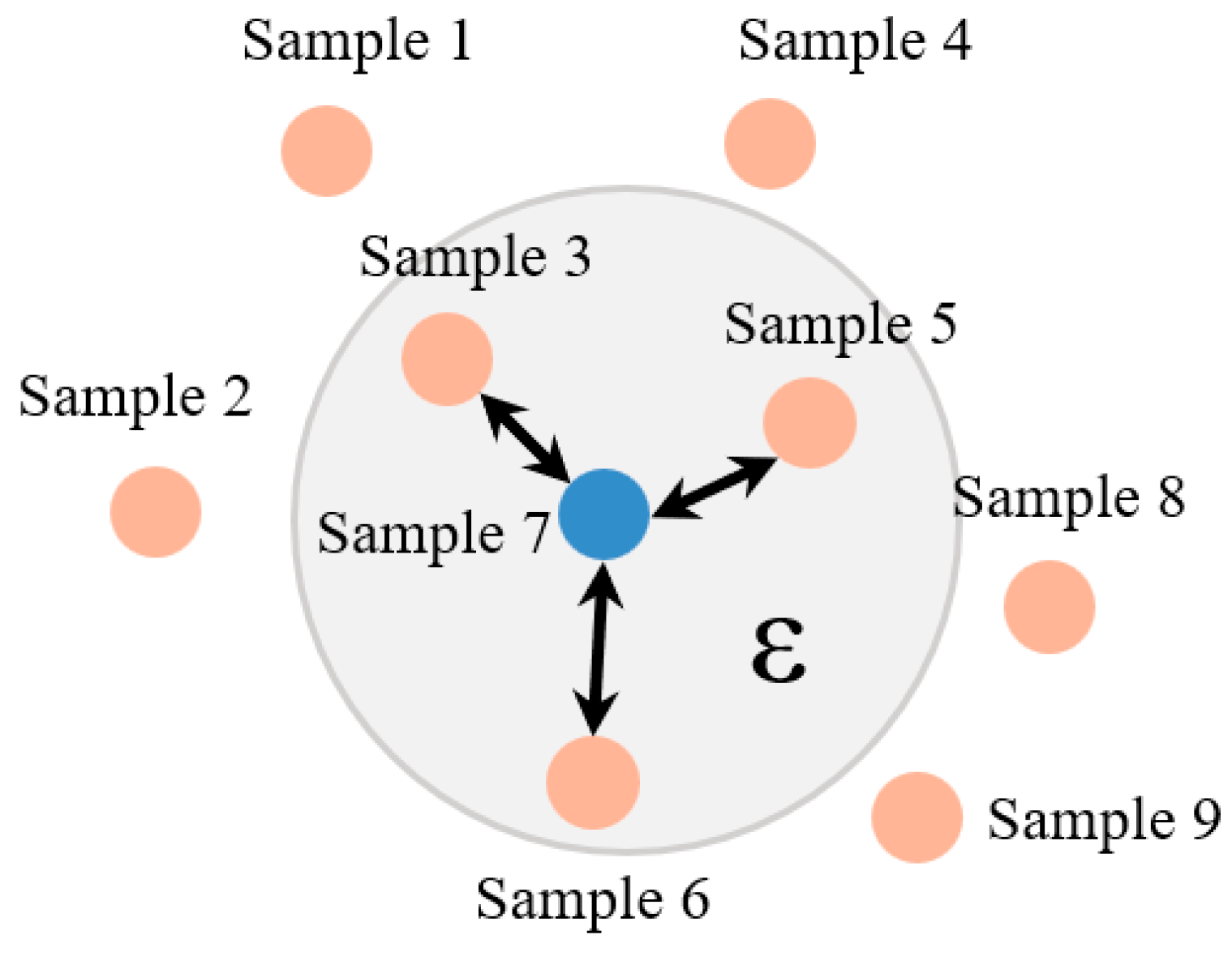
Accordingly, a threshold $\epsilon$ is defined: if $\rho (x_i,x_j)>\epsilon$, an edge is considered to exist between the i-th and j-th samples; otherwise, no edge connects these two samples, as illustrated in Figure 2.

2.3. Path Graph

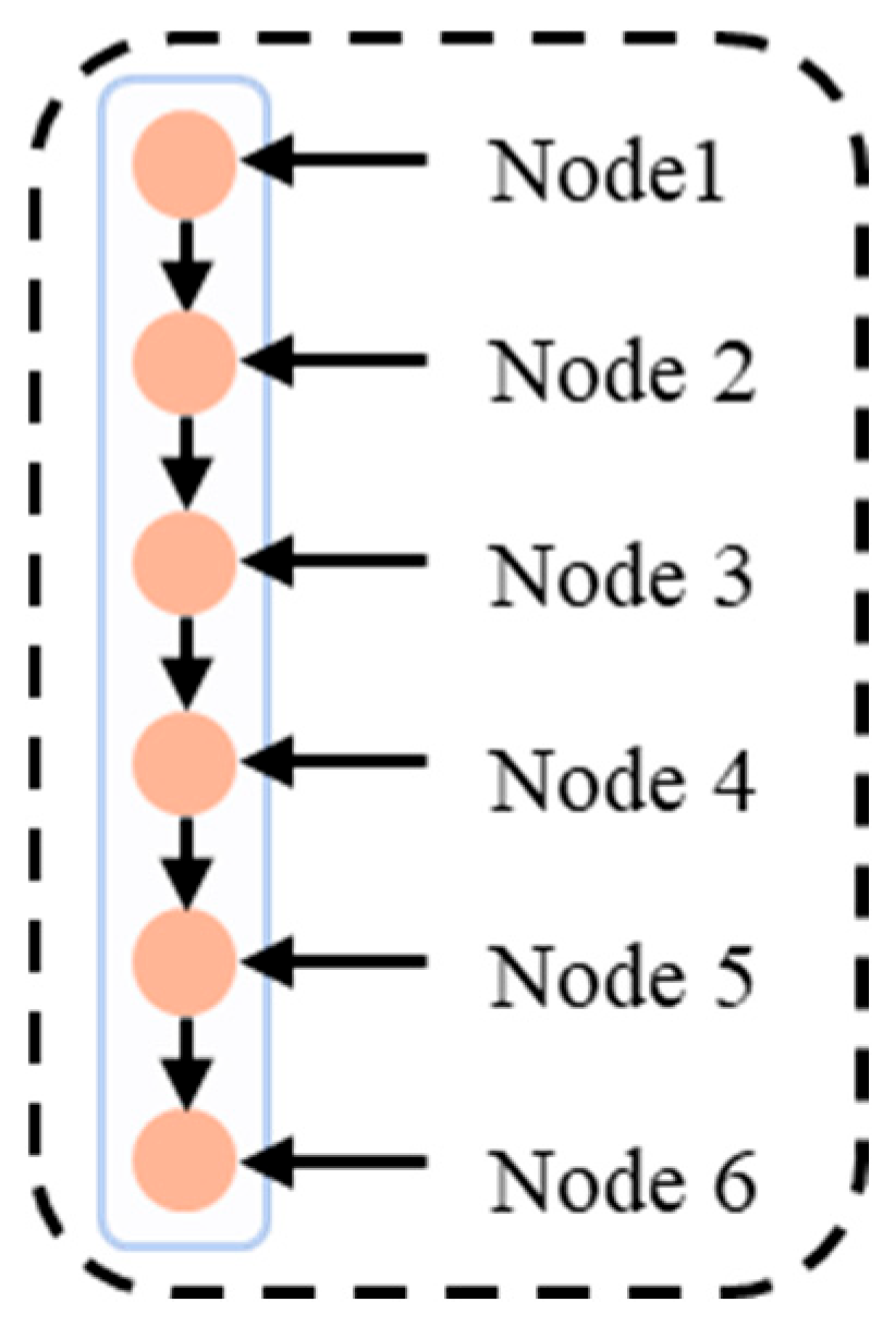
The path graph structure is a fundamental topology for modeling sequential dependencies among the samples. Its construction begins by randomly shuffling all samples into a new, randomized sequence. This critical randomization step ensures the resulting path is impartial and mitigates any inherent biases present in the original data arrangement. Subsequently, a single edge is established sequentially between every pair of adjacent samples in the new ordered sequence. The resulting graph forms a linear structure with a maximum node connectivity of two, as illustrated in Figure 3. This topology effectively models a simple, linear, and non-cyclical dependency flow, thus making it suitable for capturing global relationships across the entire dataset [33].

2.4. DeepWalk Algorithm

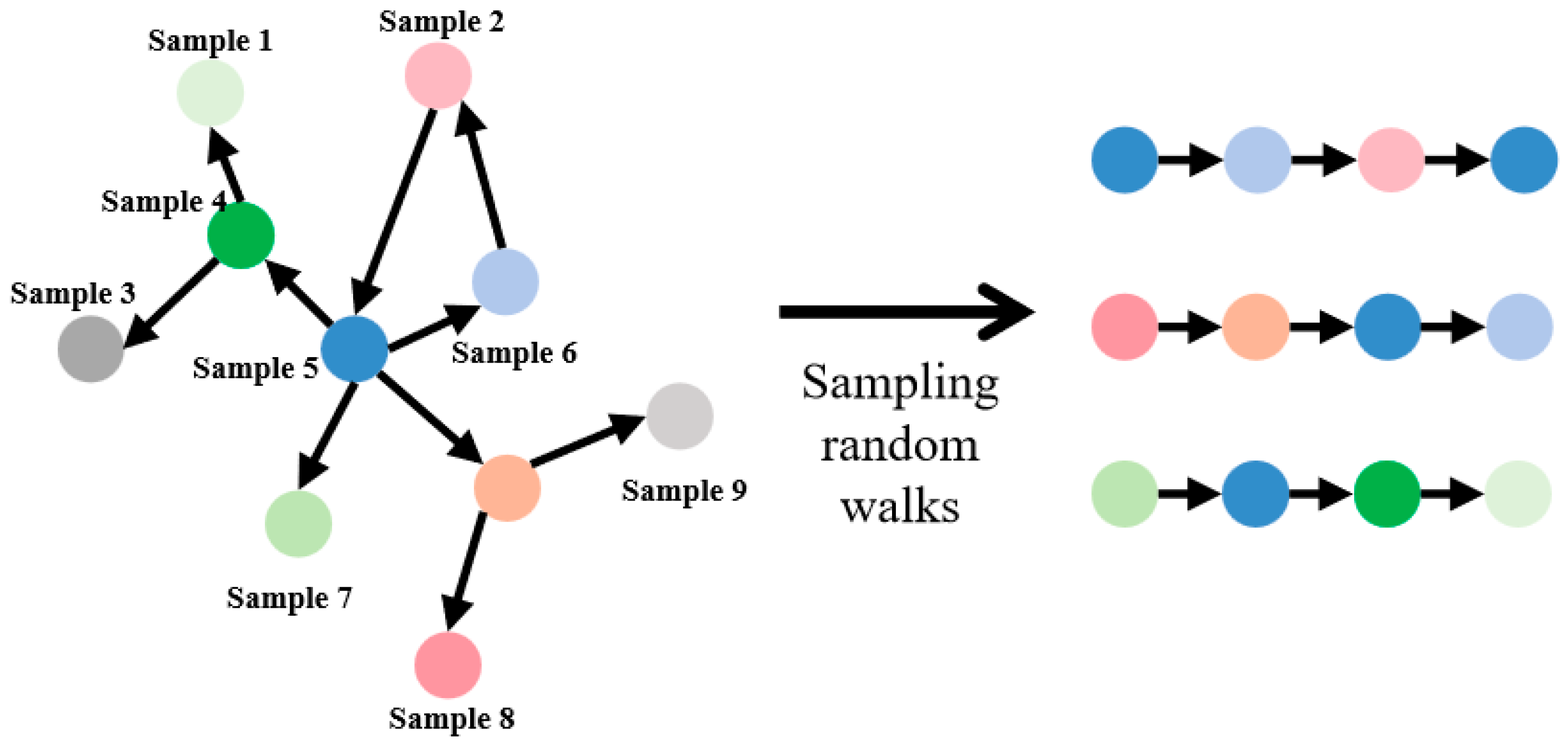
DeepWalk is an unsupervised graph embedding algorithm, with the core idea of drawing an analogy between graph-structured data and natural language processing models. The algorithm treats nodes visited during the random walk as words and the node sequences generated as sentences, thus converting the graph structure into a virtual corpus [34]. The implementation of the algorithm involves two key steps: node sampling and node embedding. In the node sampling stage, many node sequences are generated in the graph using a random walk strategy, as shown in Figure 4. The starting points and walking paths of these sequences are randomly determined to ensure the global sampling of the entire graph [33]. The process code is shown in

Table 1. The pseudocode of the DeepWalk algorithm.

Algorithm Name	$\mathbf{DeepWalk}$
Input:	Graph data:  $G(V,E)$ Window Size: $\omega$ Embedding Size: $d$ Steps: $\gamma$ Walk Length per vertex: $t$
Output:	Node embedding matrix: $\Phi \in {ℝ}^{\left|V\right|\times d}$ 1. Initialize: Sample $\Phi \mathrm{from}{\mathrm{U}}^{\left|V\right|\times d}$ 2. Build a binary tree from V 3. $\mathrm{for}i=0$ to $\gamma$ do 4.      $O=shuffle(V)$ 5.      $\mathrm{for}\mathrm{each}{v}_i\in O$ do 6.         $W_{v_i}=RandomWalk(G,V_i,t)$ 7.         $SkipGram(\Phi ,W_{v_i},\omega )$ 8.       end for 9. end for

.

In the node embedding stage, the Skip-Gram model from Word2Vec is used to learn the node sentences, thus resulting in a low-dimensional vector representation for each node. The algorithm flow is shown in

Table 2. The pseudocode of the Skip-Gram algorithm.

Algorithm Name	$\mathbf{Skip}\text{-}\mathbf{Gram}$
Output:	1. for each $v_j\in W_{v_i}$ do 2.     for each $u_k\in W_{v_i}[j-w:j+w]$ do 3.            $J(\Phi )=-\log \mathrm{Pr}(u_k|\Phi (v_j))$ 4.            $\Phi =\Phi -\alpha \times {\displaystyle \frac{\partial J}{\partial \varphi }}$ 5.       end for 6. end for

.

The Skip-Gram model normalizes the feature vectors from the mapping layer into a probability distribution vector using the Softmax activation function, in which the sum of all probabilities equals 1. The probability distribution formula is as follows [35]:

$$\sigma \left(x_i\right)={\displaystyle \frac{x^{z_i}}{{\displaystyle \sum _{j=1}^K{x}^{z_j}}}}$$

(6)

For a given training sample, the objective of the model is to maximize the probability of the true context words $y_j^{*}$, i.e.,

$$\max y_j^{*}=\max \left[{\displaystyle \frac{e^{x_j^{*}}}{{\displaystyle \sum _{j=1}^V{e}^{x_j}}}}\right]$$

(7)

For optimization convenience, the maximization problem is converted into an equivalent minimization problem. The negative log-likelihood (i.e., cross-entropy loss) is used as the loss function $E$. Since the logarithm of $y_j$ is negative, the target is converted into a minimization problem by taking the negative of the log-likelihood:

$$\max {\displaystyle \frac{e^{x_j^{*}}}{{\displaystyle \sum _j{e}^{x_j}}}}=\min \left(-\log {\displaystyle \frac{e^{x_j^{*}}}{{\displaystyle \sum _j{e}^{x_j}}}}\right)=\min \left(\log {\displaystyle \sum _{j=1}^V{e}^{x_j}}-x_j^{*}\right)$$

(8)

This gives the model’s loss function $E$ as follows:

$$E=\log {\displaystyle \sum _{j=1}^V{e}^{x_j}}-x_j^{*}$$

(9)

We then compute the partial derivative of $E$ with respect to $x_j$ and define the result as the following:

$$e_j={\displaystyle \frac{\partial E}{\partial x_j}}={\displaystyle \frac{\partial }{\partial x_j}}\left(\log {\displaystyle \sum _{j=1}^V{e}^{x_j}}\right)-{\displaystyle \frac{\partial x_{j^{*}}}{\partial x_j}}=y_j-{\displaystyle \frac{\partial x_j^{*}}{\partial x_j}}$$

(10)

2.5. Extreme Learning Machine

The ELM (extreme learning machine) is an efficient machine learning algorithm based on feedforward neural networks. Its core idea is to use randomly generated input weights directly as the weights from the input layer to the hidden layer, thus eliminating the time-consuming iterative parameter tuning process found in traditional backpropagation algorithms. This characteristic allows the ELM to train extremely fast while maintaining good generalization performance. For a dataset with N samples $(x_i,y_j)\in R^n\times R^m$, the output of a single-hidden-layer feedforward network (SLFN) with L hidden layer nodes can be represented as follows [36]:

$$f_L\left(x_i\right)={\displaystyle \sum _{i=1}^N{\beta }_i}G\left({\omega }_i\cdot x_i+b_i\right)=y_j,j=1,2,\dots ,N$$

(11)

where $w_i$ represents input weights; $b_i$ denotes hidden layer neuron thresholds; ${\beta }_i$ refers to connection weights between the i-th hidden neuron and the output layer; and $G\left(\cdot \right)$ is the activation function of the hidden layer neurons.

We then rewrite Equation (11) in matrix form:

$$\min {‖H\beta -Y‖}^2$$

(12)

$$H={\left(\begin{array}{ccc}G\left({\omega }_1,b_1,x_1\right)& \dots & G\left({\omega }_L,b_L,x_L\right)\\ ⋮& \ddots & ⋮\\ G\left({\omega }_1,b_1,x_N\right)& \dots & G\left({\omega }_L,b_L,x_N\right)\end{array}\right)}_{N\times L}$$

(13)

$$\beta ={[{\beta }_1,{\beta }_1,\dots ,{\beta }_L]}_{L\times m}^T;Y={[y_1,y_1,\dots ,y_L]}_{L\times m}^T$$

(14)

In the ELM, since the input weights $w_i$ and biases $b_i$ are randomly generated and then fixed, the hidden layer output matrix $H$ becomes a fixed constant matrix. At this point, the weight matrix $\beta$ connecting the hidden layer and the output layer can be obtained by solving the least squares problem of the linear system $H\beta =Y$. Its analytical solution is as follows:

$$\widehat{\beta }=H^{+}Y$$

(15)

where $H^{+}$ is the Moore–Penrose pseudoinverse of the hidden layer output matrix.

Finally, the predicted output of the trained ELM model for a new sample $x$ is as follows:

$$f(x)=H(x)\times \beta$$

(16)

3. Fault Recognition Method Based on DWELM

3.1. Method

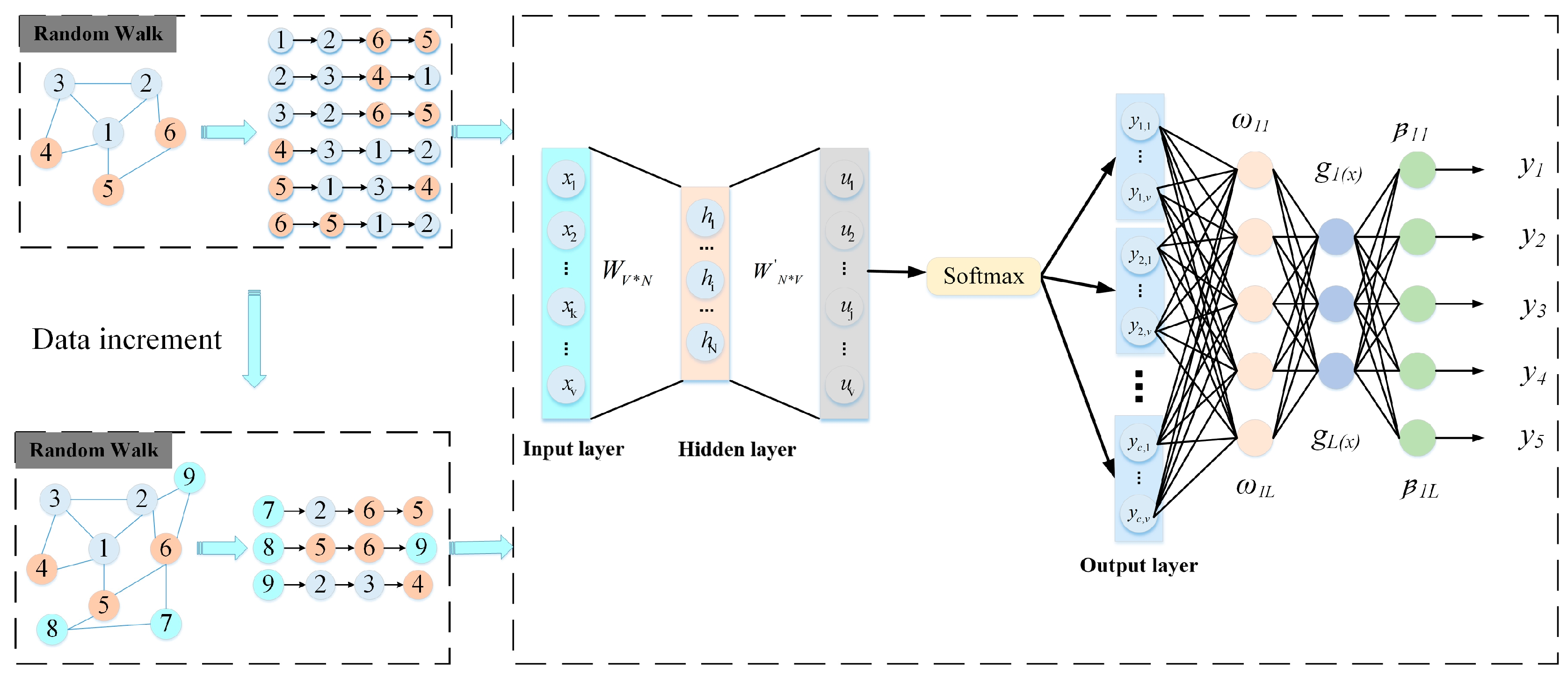
The DWELM diagnostic model consists of two core components: the DeepWalk graph embedding feature extraction layer and the extreme learning machine (ELM) classifier layer. Its overall structure is shown in Figure 5 [33]. The main steps of the model’s method are as follows:

Step 1: Graph Structure Construction: The collected continuous vibration signal stream is divided into data segments, and a dynamically evolving k-nearest neighbor graph model is constructed for each data segment.

Step 2: Graph Embedding Feature Extraction: Random walks are performed on the constructed graph to generate many node sequences, thus capturing the local topological structure and contextual information. The Skip-Gram model is used to train the node sequences, mapping each node in the graph to a low-dimensional, dense feature vector, thus converting the graph structure into numerical features.

Step 3: Fault State Recognition: The node embedding vectors are used as features and input into the ELM classifier for training, thereby enabling the rapid and accurate recognition of fault states for each node.

Step 4: Online Incremental Update: When new monitoring data is introduced, it is added as a new node to the existing graph. The new node and its local neighborhood undergo Steps 2 to 4 again. The embedding vectors of a few old nodes directly connected to the new node are fine-tuned, while the majority of the old node representations remain unchanged, thus enabling efficient and adaptive online learning.

3.2. Model Training Parameter Settings

During model construction, the following key parameters were set to improve the comprehensibility and reproducibility of this study, as listed in

Table 3. Model parameter settings.

Parameter	Value	Parameter Description
Number of random walk sequences	30	The number of random walk paths that started from each node, affecting the coverage and sampling sufficiency of node sequences.
Maximum length of random walk sequences	15	The maximum number of steps in each random walk path, controlling the trade-off between local and global structural information.
Sliding window size	15	The context window size used in the Skip-Gram model, influencing the model’s ability to capture local node relationships.
Node embedding dimension	128	The length of the node embedding vector, determining the dimensionality and expressive power of the feature representation.
ELM hidden layer number	400	The number of neurons in the hidden layer of the extreme learning machine, affecting the model’s nonlinear fitting capability and classification performance.

: the number of random walk sequences, the maximum sequence length, the node embedding dimension, and the sliding window width.

4. Experiment and Analysis of Results

4.1. Description of Southeast University Gearbox Dataset

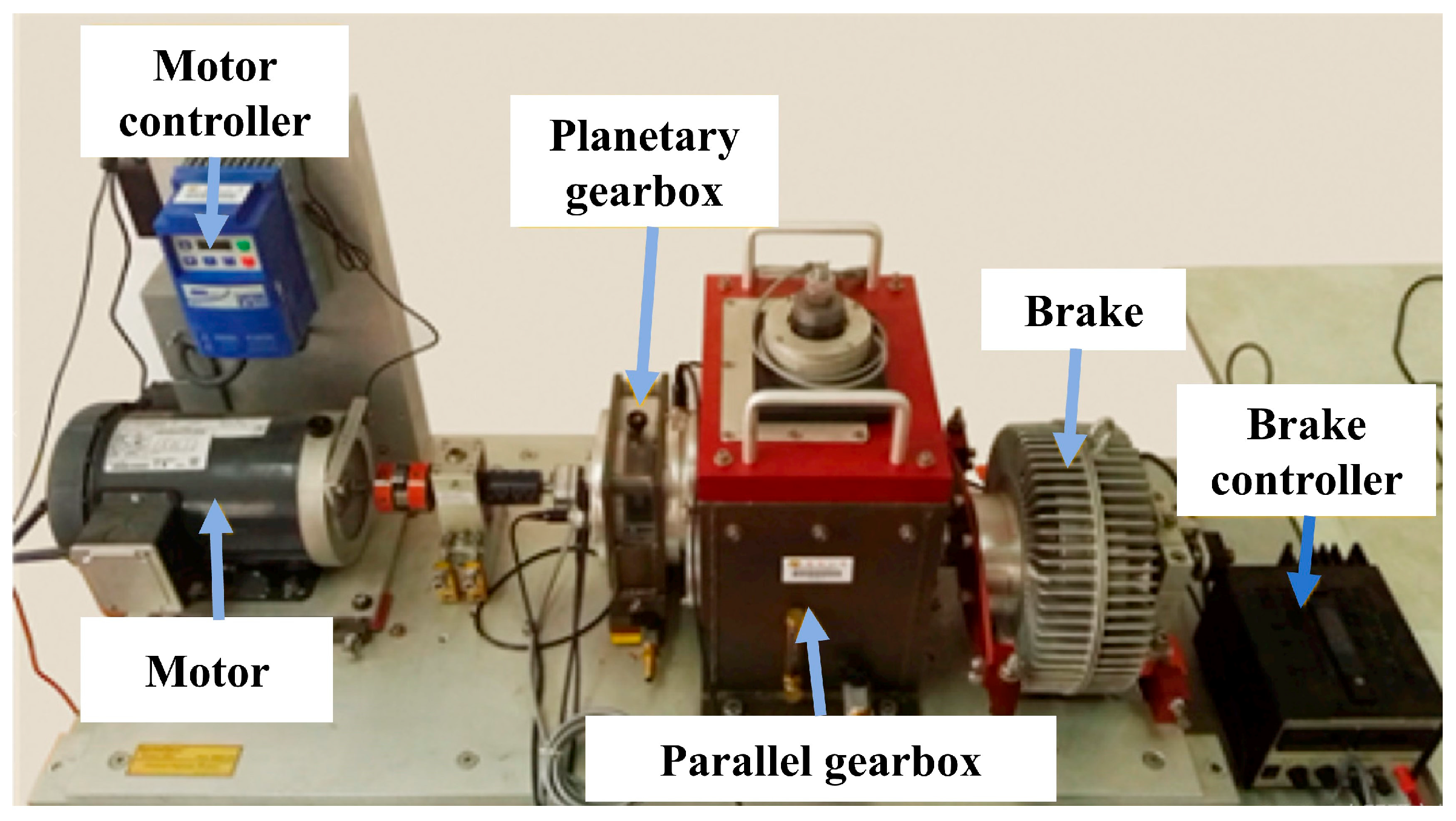
To validate the proposed method, experimental data from the Southeast University gearbox dataset were used. This dataset includes five different conditions: chipped, tooth breakage, root crack, tooth surface wear, and normal conditions. The corresponding operating conditions for each fault type are shown in

Table 4. Fault description of Southeast University gearbox dataset.

Fault Status	Condition 1	Condition 2
Health	1200 rpm and 0 Nm	1800 rpm and 7.32 Nm
Chipped
Miss
Root
Surface

[37]. The experimental setup includes a motor, motor controller, planetary gearbox, reduction box, brake, and its controller, as shown in Figure 6.

4.2. Description of HUST Gearbox Dataset

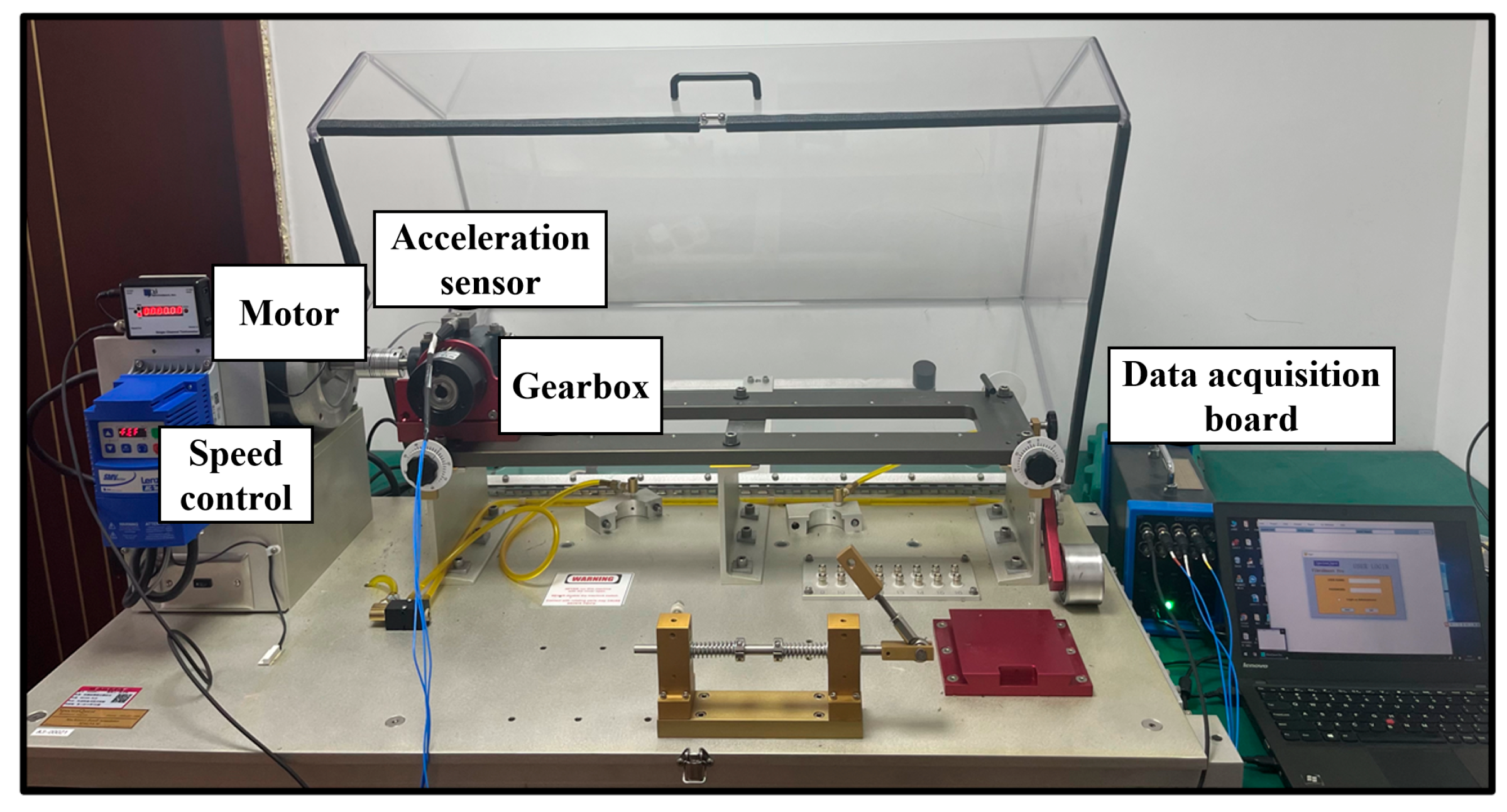
The gearbox experimental platform from Huazhong University of Science and Technology (HUST) consists of a speed controller, a motor, a gearbox, and an accelerometer, as illustrated in Figure 7 [38]. The dataset covers the healthy state of the gears as well as two common types of faults: broken tooth and missing tooth. Under four operating conditions with different speeds and loads, normal vibration signals and two patterns of tooth breakage and tooth loss failure were collected. The detailed fault descriptions of the gearbox dataset are presented in

Table 5. Fault description of HUST gearbox dataset.

Fault Status 1	Fault Status 2	Load	Rotate Speed
Broken tooth	Missing tooth	0.113 Nm 0.226 Nm 0.339 Nm 0.452 Nm	1500 rpm 1800 rpm 2100 rpm 2400 rpm

.

4.3. Experimental Sample Division

In the Southeast University dataset, the vibration signals are divided into several data segments, each containing 1000 sampling points, which are treated as one sample. Studies have shown that similar dimension parameters can achieve a balance between resolution and computational feasibility [39]. Therefore, in this research, a 1000-point analysis window was used, aiming to match the physical dynamics of the transient fault characteristics during the sensing activation process. A total of 5240 samples were collected for five states of each gearbox type. The HUST dataset contains 786 samples. To verify the online learning performance of the proposed method, each dataset is divided into four stages for online learning. For the Southeast University dataset, the first stage uses 1310 samples for online learning, the second stage adds 1310 new samples, and so on, until all four stages are completed. The same division strategy is applied to the HUST dataset. The final dataset description is shown in

Table 6. Description of experimental samples.

Dataset	Fault Status	Label	Number of Samples	Total
Southeast University	Health	0	1048	5240
	Chipped	1	1048
	Miss	2	1048
	Root	3	1048
	Surface	4	1048
HUST	Normal	0	262	786
	Broken_tooth	1	262
	Missing_tooth	2	262

.

4.4. Results Analysis and Discussion

4.4.1. Southeast University Dataset Experimental Results and Analysis

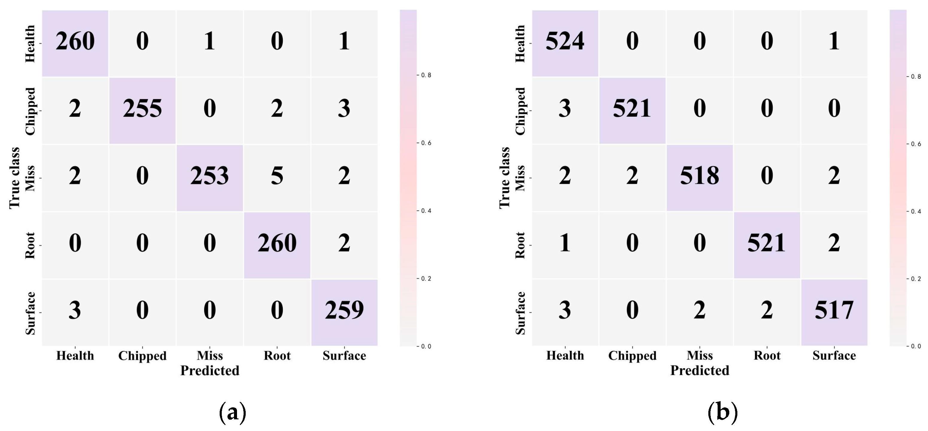
To verify the robustness of the DWELM model under different operating conditions, this study investigated the state recognition ability of the model using data from two operating conditions in the Southeast University dataset. In practical operation, equipment may first run under operating condition 1 for some time and then switch to operating condition 2. First, a graph structure containing 1130 nodes was constructed based on 1310 samples from operating condition 1. Subsequently, 1310 samples from operating condition 2 were added to the graph, thus increasing the total number of nodes in the graph structure to 2620. A total of 10 repeated experiments were conducted on this data to assess the model’s recognition performance, and the results are shown in Figure 8.

The experimental results show that the proposed method demonstrates excellent performance under both single and mixed operating conditions. Using only 1130 samples from operating condition 1, the recognition accuracy reaches 98.24%. When the sample size is expanded to 2260 mixed condition samples, thus covering both operating conditions 1 and 2, the accuracy further increases to 98.41%. This indicates that the method has outstanding accuracy and robustness, effectively adapting to changes in different operating conditions.

4.4.2. HUST Dataset Experimental Results and Analysis

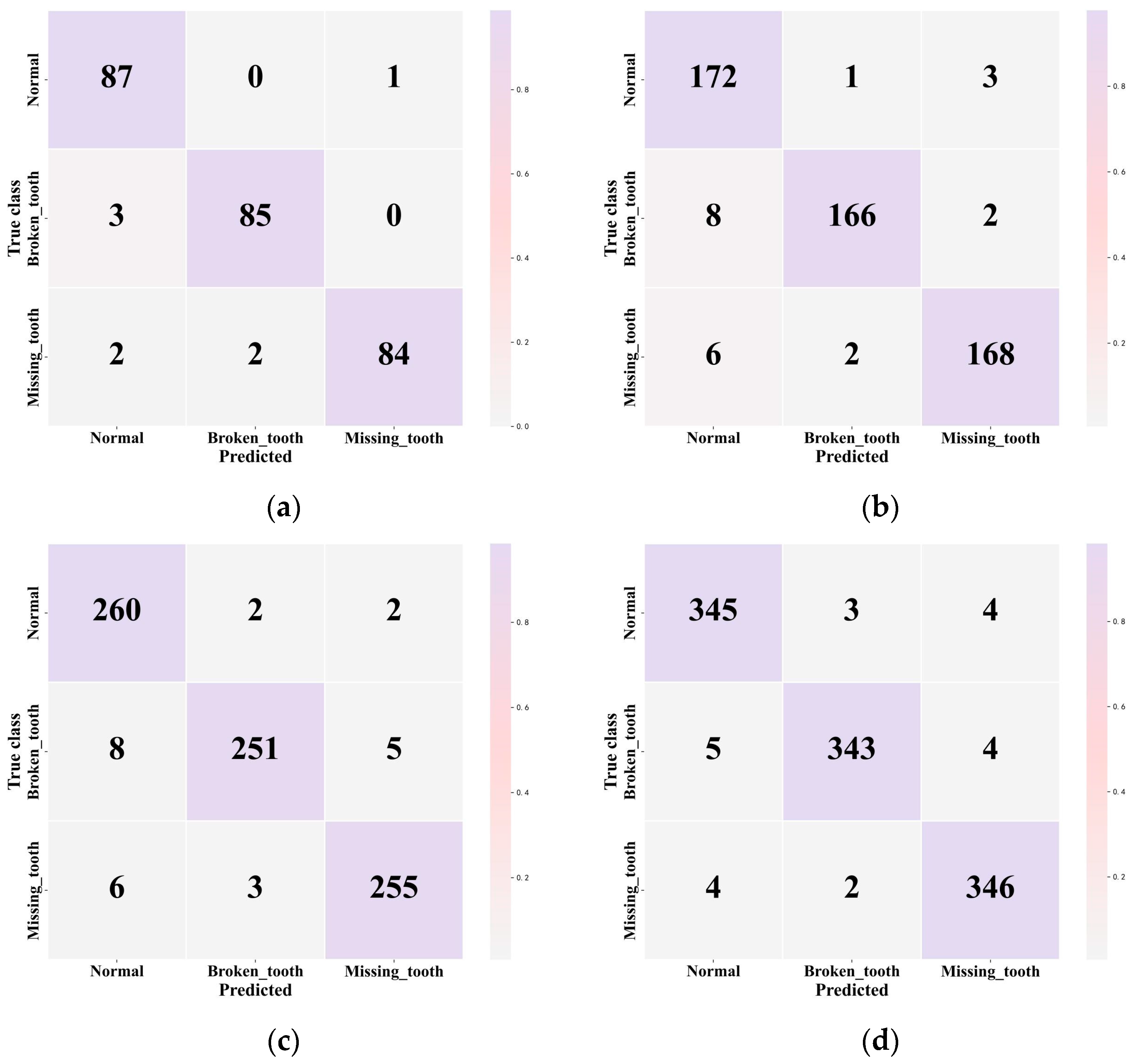
To verify the recognition performance of the DWELM model under different operating conditions, this study investigated its online state recognition ability across four operating conditions of the HUST dataset. First, a k-nearest neighbor graph containing 264 nodes was constructed using 264 sample segments from operating condition 1. Subsequently, 264 samples from operating conditions 2, 3, and 4 were added sequentially, thus gradually expanding the graph structure. As a result, the total number of nodes increased to 528, 792, and 1056, respectively. Based on the constructed graph structure, a total of 10 repeated experiments were conducted, and the recognition results are shown in Figure 9.

The experimental verification results show that under a single operating condition, the model achieves an accuracy of 96.97%, as shown in Figure 9a. When operating condition 2 is added for mixed training, the accuracy slightly drops to 95.83%, which is likely due to the initial adaptation burden caused by differences in feature distribution between the conditions. However, as more operating conditions are added, the accuracy increases to 96.72% and further rises to 97.91% after adding operating condition 4. This improvement indicates that the model has incremental learning capabilities and can gradually enhance its generalization performance by being exposed to more operating condition data.

The confusion matrix results show that recognition of the normal state (healthy state) is consistently the most stable, with extremely high classification accuracy across all four scenarios. Only a few instances are misclassified as Broken_tooth or Missing_tooth. There is some confusion between Broken_tooth and Missing_tooth in the early mixed operating conditions. For example, eight instances of Broken_tooth were misclassified as normal and two as Missing_tooth. Additionally, six instances of Missing_tooth were misclassified as Broken_tooth, as shown in Figure 9b. However, as more operating conditions are added, the confusion between these two types of faults is significantly reduced, as shown in Figure 9c,d. Especially with the four-condition mixture, the model’s discrimination of the three fault categories becomes clearer, thus indicating that the model progressively enhances its ability to capture subtle fault features through multi-condition fusion learning.

4.4.3. Visualization Analysis

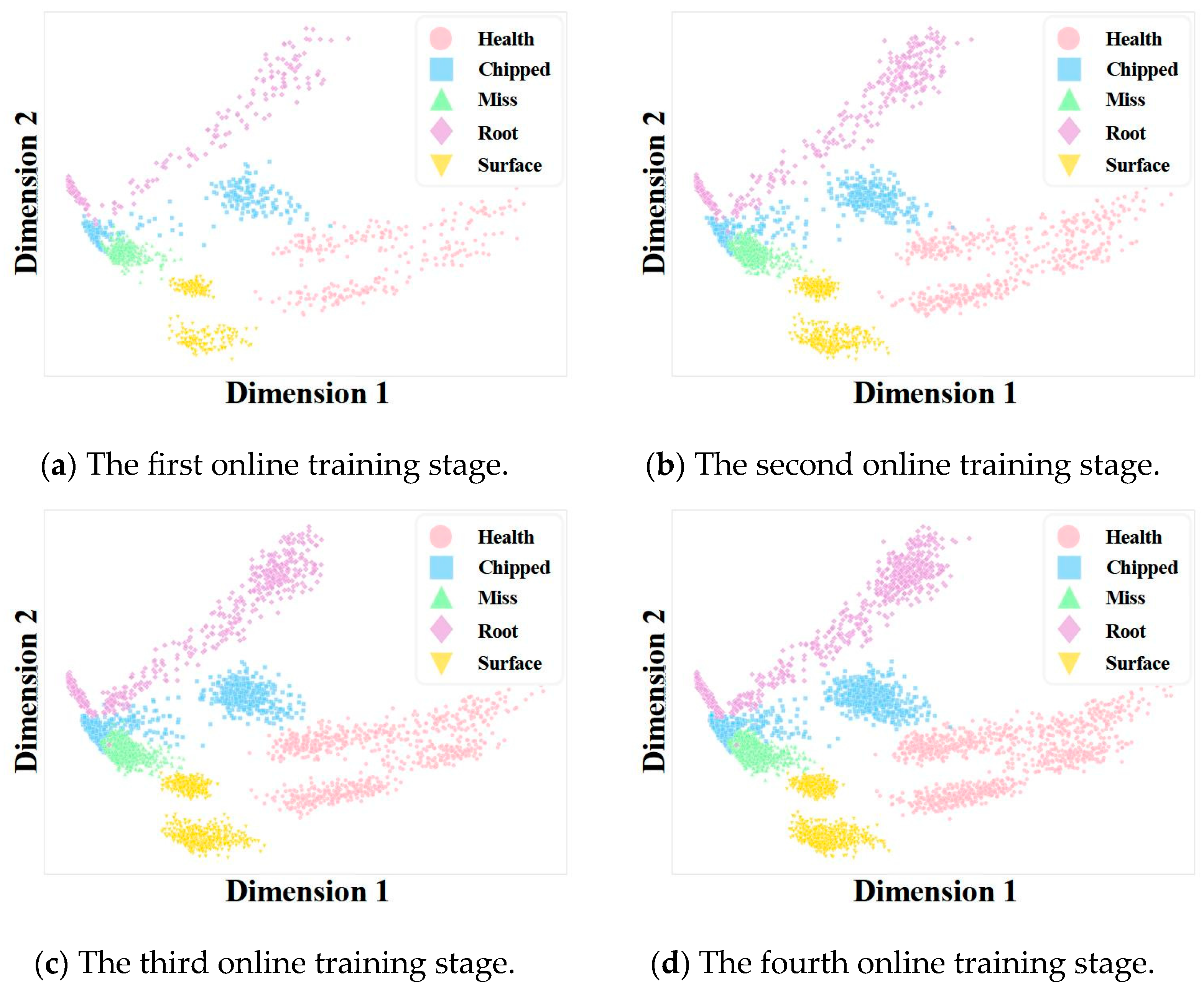
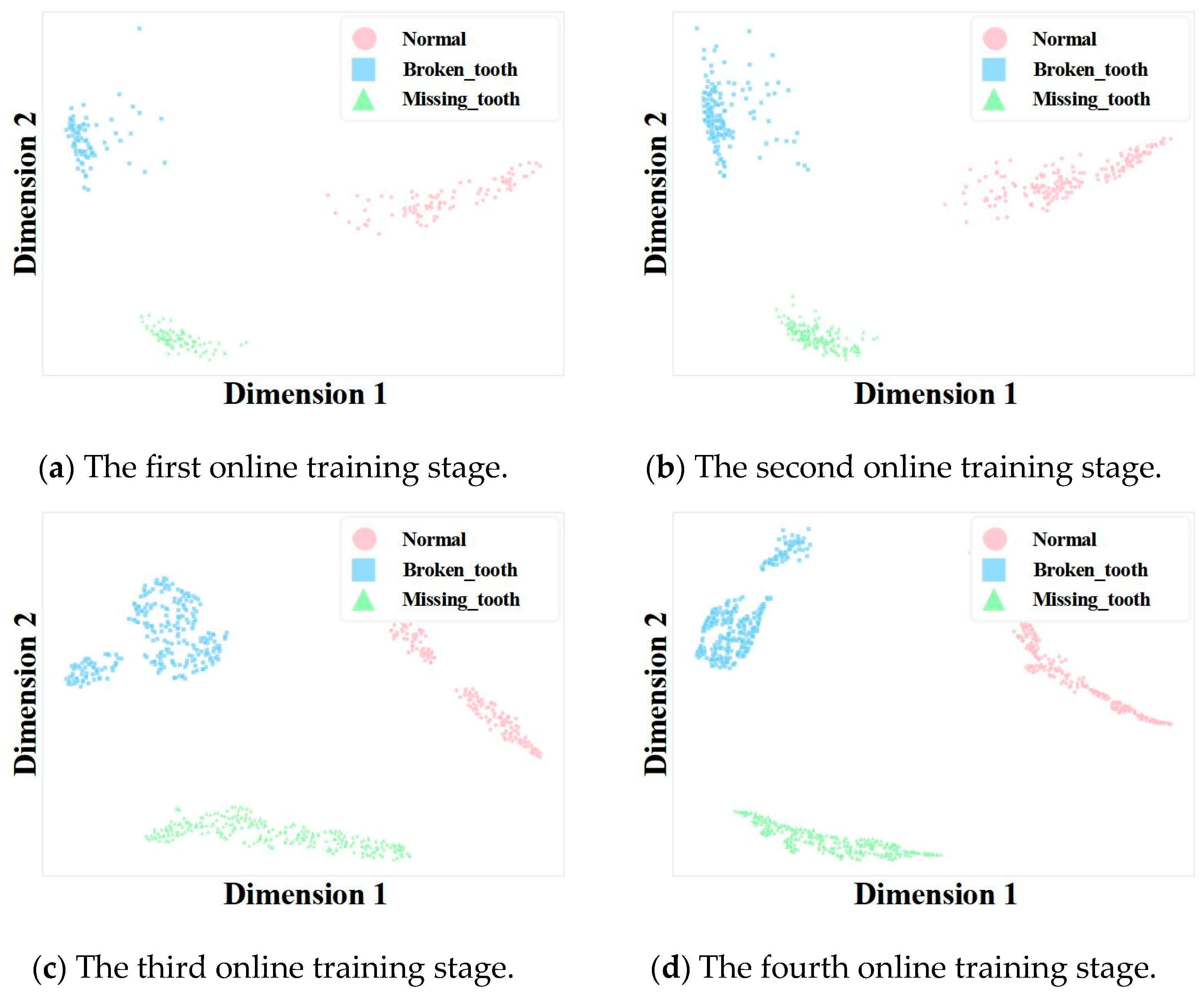
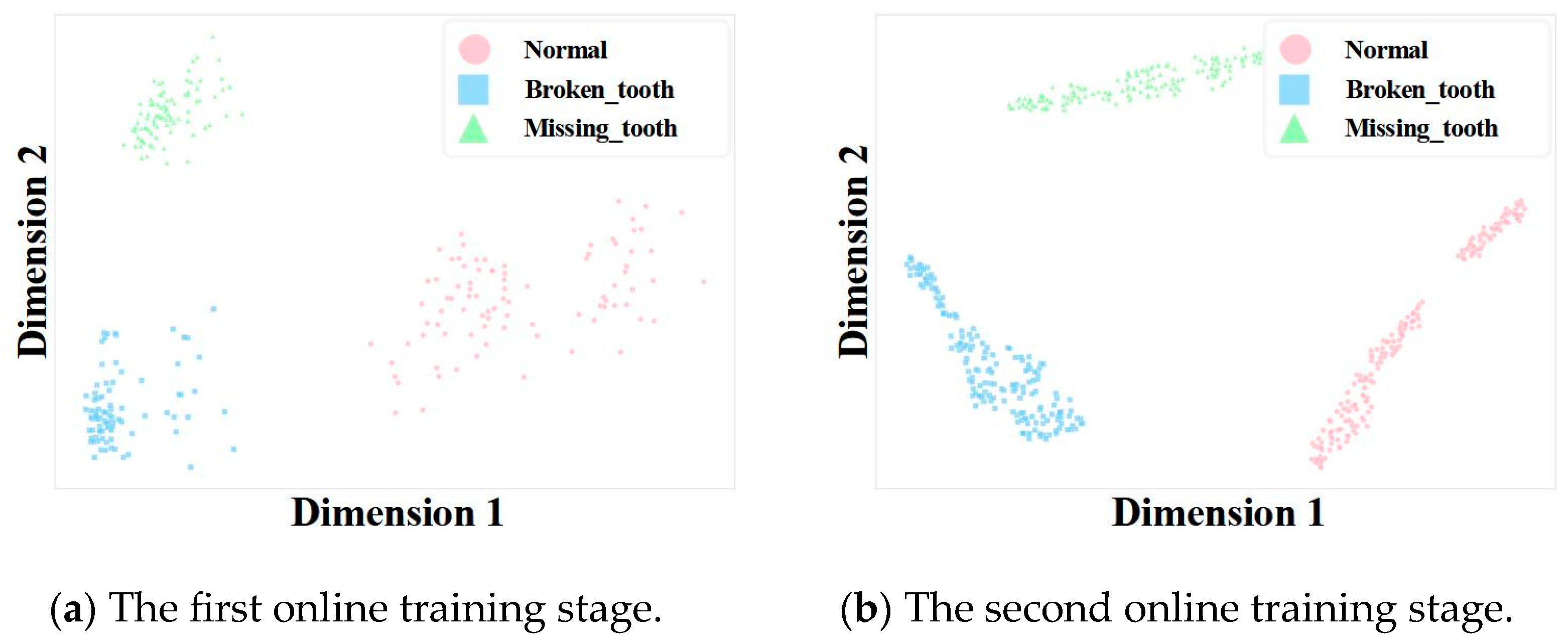
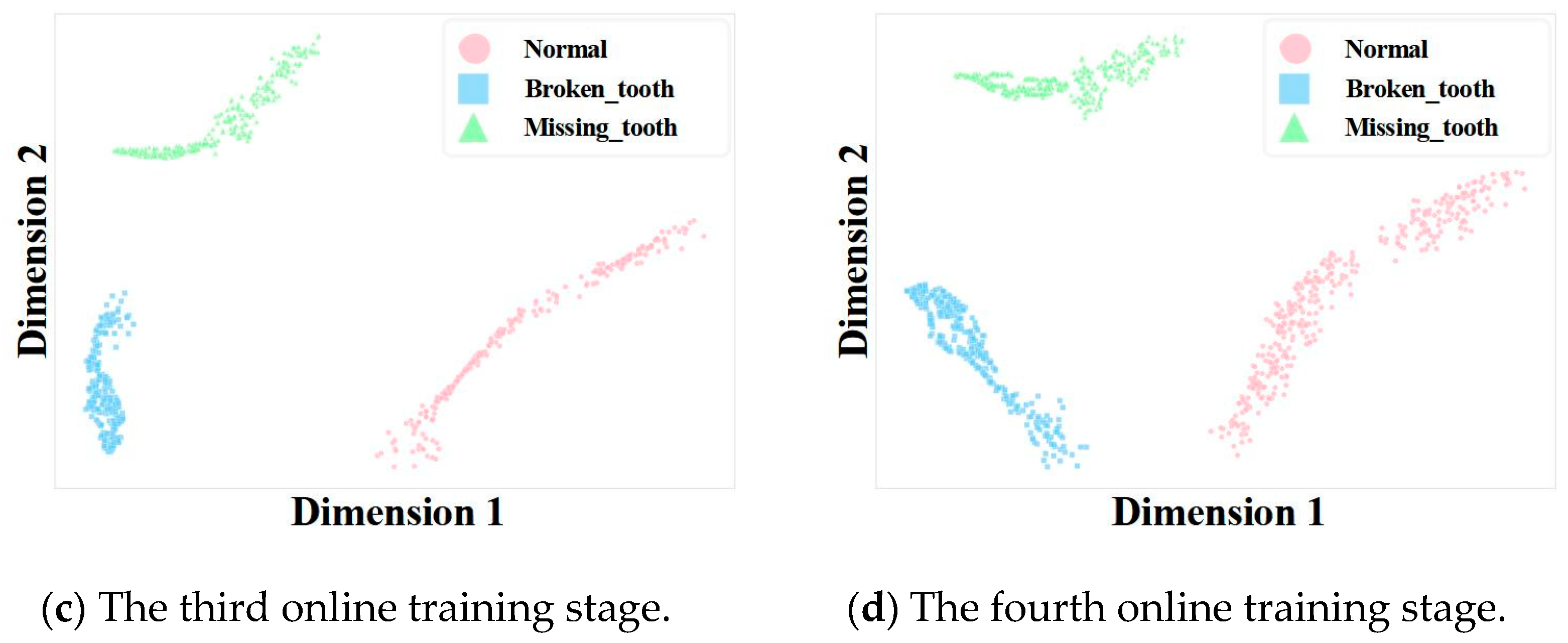
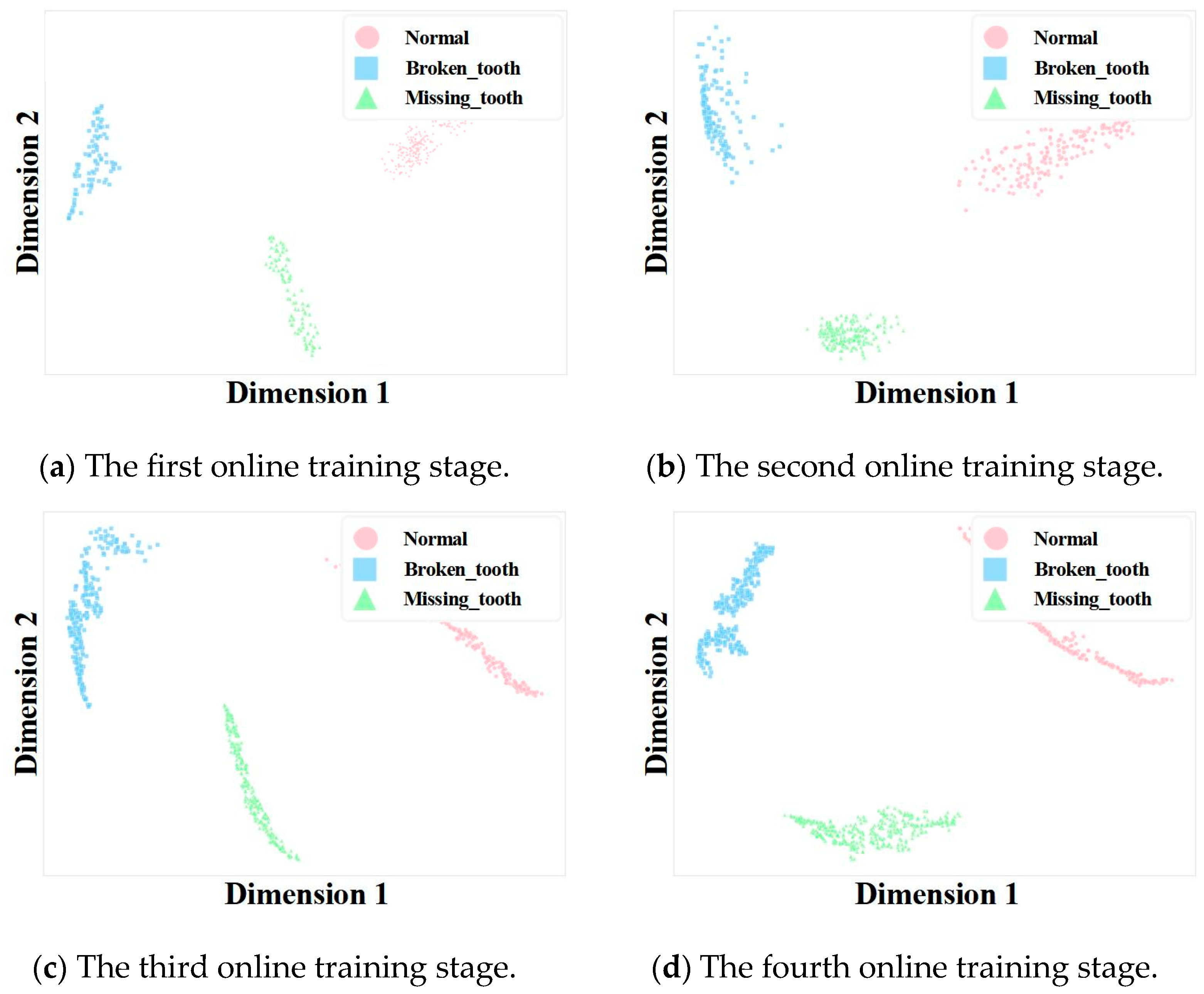
To further illustrate the effectiveness of the DeepWalk model in online training for gearbox fault recognition, the T-SNE algorithm is used for a visual analysis of the feature extraction performed by the DeepWalk model with each increment in data points. First, the features of the graph structure data composed of the first set of data are visualized. After adding the second set of data to the graph structure, the features are visualized again, and this process is repeated with each subsequent dataset. The experimental results are shown in Figure 10, Figure 11, Figure 12, Figure 13, Figure 14 and Figure 15.

In the four online learning stages of operating conditions 1 and 2 of the Southeast University dataset, the classification performance shows a continuous trend of improvement. In the initial stage, some overlap occurs between the categories, especially between the fault categories and the normal state, thus resulting in slight confusion. This is mainly because the model failed to learn the distinguishing features between different fault modes during the initial training stage. Since the graph structure was constructed using limited data at this early stage, the node embeddings were unable to fully capture the subtle differences among various categories. As the number of learning iterations increases, intra-category cohesion improves, and the boundaries gradually become clearer. This indicates that the model effectively absorbed the newly added information, enhancing its feature discriminability. These results demonstrate that the embedding learning mechanism of DeepWalk for graph-structured data can capture the deep connections between nodes, thus maintaining high discriminability even in complex data distributions.

The online learning training results for conditions 1 through 4 of the HUST dataset demonstrate a consistent trend of progressive optimization across four iterative learning cycles. In the initial online learning phase, model performance was generally basic, with relatively low performance metrics, which can be attributed to model initialization and insufficient data. As new data were introduced and parameters were updated in the second and third online learning phases, the model’s adaptability improved significantly, thus leading to a marked enhancement in performance. By the fourth learning cycle, model performance stabilized or reached its peak, indicating that the online learning process effectively facilitated model convergence and generalization. A comparative analysis across different conditions revealed consistent model performance under conditions 3 and 4, underscoring its robustness and adaptability, which are likely attributable to high data quality and well-calibrated algorithmic parameters.

4.4.4. Graph Construction Analysis

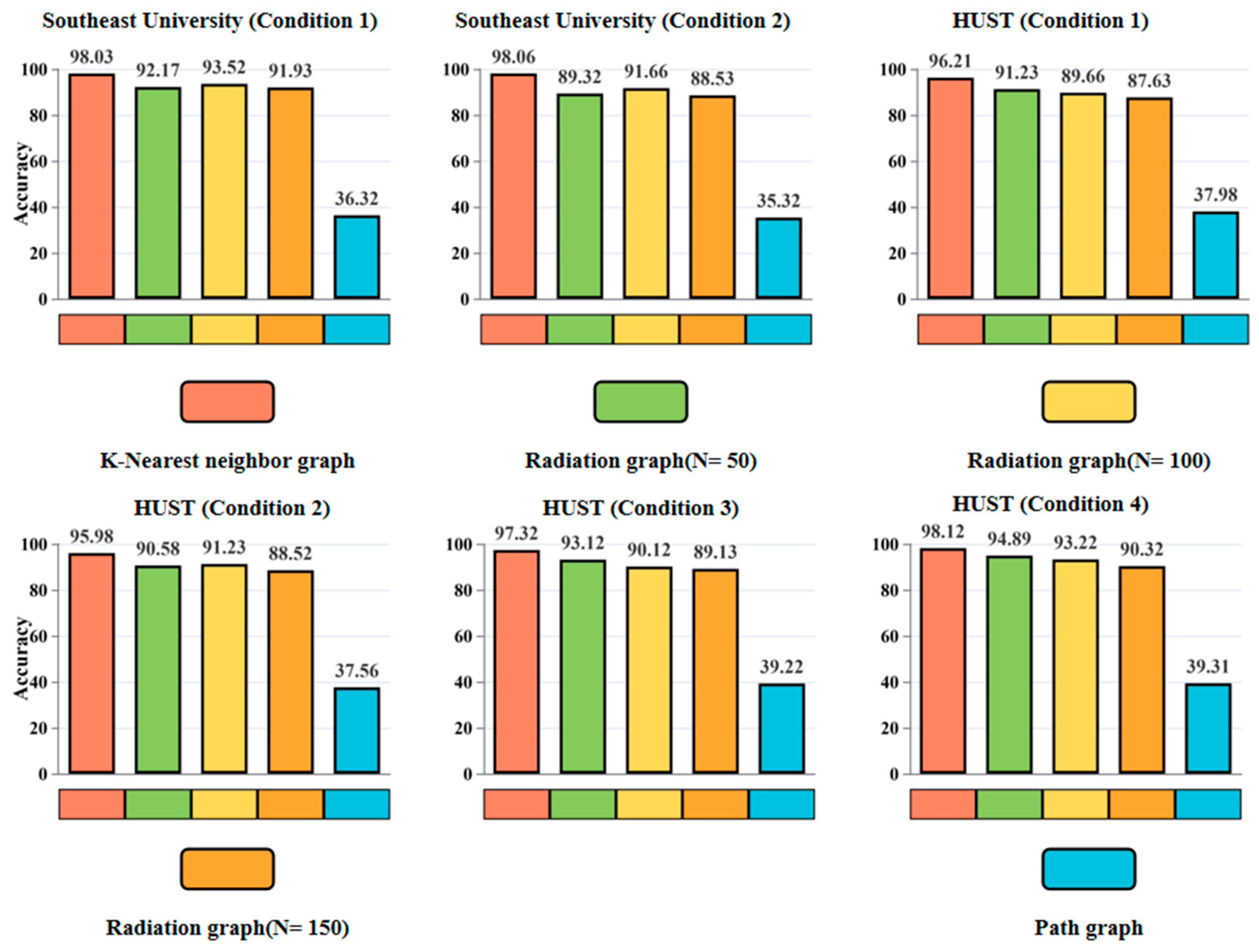
The results shown in Figure 16 indicate that all three graph construction methods achieve good fault diagnosis performance across all datasets and experimental conditions, with accuracy generally exceeding 80% and surpassing 90% in most cases. This suggests that the graph construction methods play a crucial role in the DWELM model. However, there are significant performance differences between the methods, and their performance fluctuates with changes in the dataset and conditions. A comprehensive analysis reveals that the choice of graph construction method significantly impacts the model’s performance, with its effectiveness being highly dependent on the characteristics of the dataset. Notably, the k-nearest neighbor graph outperforms the other methods in terms of fault diagnosis accuracy across all datasets, thus demonstrating the strongest robustness and generalization ability. Therefore, in subsequent research, the k-nearest neighbor graph will be used as the graph construction method, with further experiments and analysis conducted based on this approach.

4.4.5. Analysis of Classification Performance Metrics

To further quantify the classification performance of the model across different fault categories, Precision (P), Recall (R), and F1 score (F₁) were adopted as complementary evaluation metrics. These metrics, which were calculated from the confusion matrices, provide a more detailed reflection of the model’s ability to recognize each category and its error patterns. The formulas are as follows:

$$\mathrm{P}={\displaystyle \frac{\mathrm{TP}}{\mathrm{TP}+\mathrm{FP}}}$$

(17)

$$\mathrm{R}={\displaystyle \frac{\mathrm{TP}}{\mathrm{TP}+\mathrm{FN}}}$$

(18)

$${\mathrm{F}}_1=2\times {\displaystyle \frac{\mathrm{Precision}\times \mathrm{Recall}}{\mathrm{Precision}+\mathrm{Recall}}}$$

(19)

where TP, FP, and FN denote true positives, false positives, and false negatives, respectively.

(1)

Analysis for the Southeast University Dataset

The classification performance indicators of the Southeast University dataset under four different operating condition combinations were calculated and are listed in

Table 7. Classification performance metrics (%) for the Southeast University dataset under different condition sets.

Fault State	Condition 1 (%)	Condition 1–2 (%)	Condition 1–3 (%)	Condition 1–4 (%)
	Precision/Recall/F1	Precision/Recall/F1	Precision/Recall/F1	Precision/Recall/F1
Health	99.2/99.5/99.3	98.8/99.1/99.0	99.0/99.3/99.1	99.2/99.4/99.3
Broken_tooth	95.1/94.3/94.7	93.8/92.5/93.1	96.2/95.8/96.0	97.5/97.0/97.2
Missing_tooth	94.8/95.2/95.0	92.5/91.8/92.1	95.8/96.1/95.9	96.8/97.2/97.0
Root crack	96.2/95.8/96.0	94.9/95.2/95.0	97.1/96.8/96.9	98.0/97.6/97.8
Surface wear	95.5/96.0/95.7	94.1/94.5/94.3	96.5/96.9/96.7	97.8/98.1/97.9

. The results show that the model’s identification of the “healthy” state is consistently the most stable and accurate, and its F1 score always exceeds 99% in all condition combinations. With the inclusion of more mixed condition data, the model’s ability to distinguish between the easily confused fault types “broken teeth” and “missing teeth” significantly improves. For example, for the “broken teeth” category, the F1 score increased from approximately 93.1% under condition combination 1–2 to approximately 97.2% under condition combination 1–4. This highlights the optimization of the model’s discriminative ability through the incremental learning process. Overall, the macro average F1 score steadily increased from 96.2% in a single condition to 97.9% under the four mixed conditions, thus verifying the excellent online learning and generalization ability of the model.

(2)

Analysis for the HUST Dataset

The classification performance indicators of the HUST dataset are shown in

Table 8. Classification performance metrics (%) for the HUST dataset under different condition sets.

Fault State	Condition 1 (%)	Condition 1–2 (%)
	Precision/Recall/F1	Precision/Recall/F1
Normal	99.5/99.2/99.4	99.6/99.3/99.4
Broken_tooth	97.8/97.5/97.6	98.0/97.8/97.9
Missing_tooth	97.5/97.9/97.7	97.7/98.1/97.9

. The results indicate that even with a relatively small dataset, this model can demonstrate outstanding performance. Under a single condition, the model’s recognition of the “normal” state is nearly perfect (with an F1 value of 99.4%), and the F1 values for the “tooth damage” and “tooth loss” situations are both higher than 97%. When new condition data is added to form a mixed condition set, the performance indicators of all categories remain stable or show a slight improvement.

5. Conclusions

To address the challenges of online gearbox fault diagnosis, this study proposes an innovative method based on a DeepWalk graph embedding-enhanced extreme learning machine (DWELM) approach. This method dynamically constructs a k-nearest neighbor graph from streaming vibration signals and uses DeepWalk for unsupervised embedding learning to extract low-dimensional features with strong discriminative power. These features are then combined with an ELM classifier to achieve rapid fault type recognition and online incremental model updates. The experimental results show that the proposed method maintains an average diagnostic accuracy of over 95.83% across multiple operating conditions. This significantly enhances adaptability to streaming data and improves diagnostic efficiency, thus providing a reliable solution for industrial intelligent fault diagnosis. Although the proposed method achieves encouraging results, it still has minor limitations, such as the sensitivity of graph construction to the k value and reliance on manual hyperparameter tuning. Future research will focus on providing a more rigorous theoretical foundation for the method and conducting broader experiments to evaluate performance under diverse dynamic conditions. Additionally, we aim to develop adaptive graph construction techniques, integrate attention mechanisms for multi-scale feature extraction, and combine DWELM with sequential networks, such as Long Short-Term Memory (LSTM), to enhance temporal feature learning. These advancements will further substantiate the potential of DWELM as an efficient and accurate solution for online gearbox fault diagnosis within industrial intelligent maintenance systems.

References

1. Liu, R.; Yang, B.; Zio, E.; Chen, X. Artificial intelligence for fault diagnosis of rotating machinery: A review. Mech. Syst. Signal Process. 2018, 108, 33–47. [Google Scholar] [CrossRef]
2. Meng, X.; Wang, Q.; Shi, C.; Zeng, Q.; Zhang, Y.; Zhang, W.; Wang, Y. Deep Ensemble Learning Based on Multi-Form Fusion in Gearbox Fault Recognition. Sensors 2025, 25, 4993. [Google Scholar] [CrossRef]
3. Jiang, Z.; Han, Q.; Xu, X. Fault diagnosis of planetary gearbox based on motor current signal analysis. Shock Vib. 2020, 2020, 8854776. [Google Scholar] [CrossRef]
4. Mohd Amiruddin, A.A.A.; Zabiri, H.; Taqvi, S.A.A.; Tufa, L.D. Neural network applications in fault diagnosis and detection: An overview of implementations in engineering-related systems. Neural Comput. Appl. 2020, 32, 447–472. [Google Scholar] [CrossRef]
5. Jiao, J.; Zhao, M.; Lin, J.; Liang, K. A comprehensive review on convolutional neural network in machine fault diagnosis. Neurocomputing 2020, 417, 36–63. [Google Scholar] [CrossRef]
6. Zhang, Y.; Zhou, T.; Huang, X.; Cao, L.; Zhou, Q. Fault diagnosis of rotating machinery based on recurrent neural networks. Measurement 2021, 171, 108774. [Google Scholar] [CrossRef]
7. Li, J.; Cao, X.; Chen, R.; Zhang, X.; Huang, X.; Qu, Y. Graph neural network architecture search for rotating machinery fault diagnosis based on reinforcement learning. Mech. Syst. Signal Process. 2023, 202, 110701. [Google Scholar] [CrossRef]
8. Park, P.; Di Marco, P.; Shin, H.; Bang, J. Fault detection and diagnosis using combined autoencoder and long short-term memory network. Sensors 2019, 19, 4612. [Google Scholar] [CrossRef] [PubMed]
9. Zhu, J.; Jiang, Q.; Shen, Y.; Qian, C.; Xu, F.; Zhu, Q. Application of recurrent neural network to mechanical fault diagnosis: A review. J. Mech. Sci. Technol. 2022, 36, 527–542. [Google Scholar] [CrossRef]
10. Hou, J.; Lu, X.; Zhong, Y.; He, W.; Zhao, D.; Zhou, F. A comprehensive review of mechanical fault diagnosis methods based on convolutional neural network. J. Vibroeng. 2024, 26, 44–65. [Google Scholar] [CrossRef]
11. Jiao, C.; Zhang, D.; Fang, X.; Miao, Q. Ensemble of simplified graph wavelet neural networks for planetary gearbox fault diagnosis. IEEE Trans. Instrum. Meas. 2023, 72, 3529910. [Google Scholar] [CrossRef]
12. Wang, Y.; Wu, J.; Yu, Z.; Hu, J.; Zhou, Q. A structurally re-parameterized convolution neural network-based method for gearbox fault diagnosis in edge computing scenarios. Eng. Appl. Artif. Intell. 2023, 126, 107091. [Google Scholar] [CrossRef]
13. Wang, H.; Liu, Z.; Li, M.; Dai, X.; Wang, R.; Shi, L. A gearbox fault diagnosis method based on graph neural networks and Markov transform fields. IEEE Sens. J. 2024, 24, 25186–25196. [Google Scholar] [CrossRef]
14. Chen, P.; Li, Y.; Wang, K.; Zuo, M.J. An automatic speed adaption neural network model for planetary gearbox fault diagnosis. Measurement 2021, 171, 108784. [Google Scholar] [CrossRef]
15. Lei, Y.; Yang, B.; Jiang, X.; Jia, F.; Li, N.; Nandi, A.K. Applications of machine learning to machine fault diagnosis: A review and roadmap. Mech. Syst. Signal Process. 2020, 138, 106587. [Google Scholar] [CrossRef]
16. Zhang, W.; Peng, G.; Li, C.; Chen, Y.; Zhang, Z. A new deep learning model for fault diagnosis with good anti-noise and domain adaptation ability on raw vibration signals. Sensors 2017, 17, 425. [Google Scholar] [CrossRef]
17. Li, X.; Zhang, W.; Ding, Q. Cross-domain fault diagnosis of rolling element bearings using deep generative neural networks. IEEE Trans. Ind. Electron. 2018, 66, 5525–5534. [Google Scholar] [CrossRef]
18. Zhang, A.; Li, S.; Cui, Y.; Yang, W.; Dong, R.; Hu, J. Limited data rolling bearing fault diagnosis with few-shot learning. IEEE Access 2019, 7, 110895–110904. [Google Scholar] [CrossRef]
19. Sehri, M.; Varejão, I.; Hua, Z.; Bonella, V.; Santos, A.; Boldt, F.D.A.; Dumond, P.; Varejão, F.M. Towards a Universal Vibration Analysis Dataset: A Framework for Transfer Learning in Predictive Maintenance and Structural Health Monitoring. arXiv 2025, arXiv:2504.11581. [Google Scholar] [CrossRef]
20. Zachariades, C.; Xavier, V. A Review of Artificial Intelligence Techniques in Fault Diagnosis of Electric Machines. Sensors 2025, 25, 5128. [Google Scholar] [CrossRef] [PubMed]
21. Lei, Y.; Lin, J.; Zuo, M.J.; He, Z. Condition monitoring and fault diagnosis of planetary gearboxes: A review. Measurement 2014, 48, 292–305. [Google Scholar] [CrossRef]
22. Xu, X.; Huang, X.; Bian, H.; Wu, J.; Liang, C.; Cong, F. Total process of fault diagnosis for wind turbine gearbox, from the perspective of combination with feature extraction and machine learning: A review. Energy AI 2024, 15, 100318. [Google Scholar] [CrossRef]
23. Li, R.; Wang, S.; Zhu, F.; Huang, J. Adaptive graph convolutional neural networks. In Proceedings of the AAAI Conference on Artificial Intelligence, New Orleans, LA, USA, 2–7 February 2018; Volume 32. [Google Scholar]
24. Perozzi, B.; Al-Rfou, R.; Skiena, S. Deepwalk: Online learning of social representations. In Proceedings of the 20th ACM SIGKDD International Conference on Knowledge Discovery and Data Mining, New York, NY, USA, 24–27 August 2014; pp. 701–710. [Google Scholar]
25. Liu, Y.; Jin, M.; Pan, S.; Zhou, C.; Zheng, Y.; Xia, F.; Yu, P. Graph self-supervised learning: A survey. IEEE Trans. Knowl. Data Eng. 2022, 35, 5879–5900. [Google Scholar] [CrossRef]
26. Liu, X.; Zhang, Z.; Meng, F.; Zhang, Y. Fault diagnosis of wind turbine bearings based on CNN and SSA–ELM. J. Vib. Eng. Technol. 2023, 11, 3929–3945. [Google Scholar] [CrossRef]
27. Afia, A.; Gougam, F.; Rahmoune, C.; Touzout, W.; Ouelmokhtar, H.; Benazzouz, D. Gearbox fault diagnosis using remd, eo and machine learning classifiers. J. Vib. Eng. Technol. 2024, 12, 4673–4697. [Google Scholar] [CrossRef]
28. Maaten, L.; Hinton, G. Visualizing data using t-SNE. J. Mach. Learn. Res. 2008, 9, 2579–2605. [Google Scholar]
29. Khoshraftar, S.; An, A. A survey on graph representation learning methods. ACM Trans. Intell. Syst. Technol. 2024, 15, 1–55. [Google Scholar] [CrossRef]
30. Xia, F.; Sun, K.; Yu, S.; Aziz, A.; Wan, L.; Pan, S.; Liu, H. Graph learning: A survey. IEEE Trans. Artif. Intell. 2021, 2, 109–127. [Google Scholar] [CrossRef]
31. Li, K.; Zhang, H.; Lu, G. Graph entropy-based early change detection in dynamical bearing degradation process. IEEE Internet Things J. 2024, 11, 23186–23195. [Google Scholar] [CrossRef]
32. Chen, Z.; Li, K.; Lu, G. Local mean decomposition enhanced graph spectrum analysis for condition monitoring of rolling element bearings. Meas. Sci. Technol. 2025, 36, 026121. [Google Scholar] [CrossRef]
33. Li, K.; Wang, M.J.; Yuan, M.J.; Zhang, H.S.; Yuan, K.Y.; Lu, G.L. Early fault detection for rolling bearings based on one-dimensional structure graph entropy. China Mech. Eng. 2025, 36, 1–13. (In Chinese) [Google Scholar]
34. Jeyaraj, R.; Balasubramaniam, T.; Balasubramaniam, A.; Paul, A. DeepWalk with Reinforcement Learning (DWRL) for node embedding. Expert Syst. Appl. 2024, 243, 122819. [Google Scholar] [CrossRef]
35. Wang, Y.; Cui, L.; Zhang, Y. Improving skip-gram embeddings using BERT. IEEE/ACM Trans. Audio Speech Lang. Process. 2021, 29, 1318–1328. [Google Scholar] [CrossRef]
36. Wang, J.; Lu, S.; Wang, S.H.; Zhang, Y.D. A review on extreme learning machine. Multimed. Tools Appl. 2022, 81, 41611–41660. [Google Scholar] [CrossRef]
37. Shao, S.; McAleer, S.; Yan, R.; Baldi, P. Highly accurate machine fault diagnosis using deep transfer learning. IEEE Trans. Ind. Inform. 2018, 15, 2446–2455. [Google Scholar] [CrossRef]
38. Zhao, C.; Zio, E.; Shen, W. Domain generalization for cross-domain fault diagnosis: An application-oriented perspective and a benchmark study. Reliab. Eng. Syst. Saf. 2024, 245, 109964. [Google Scholar] [CrossRef]
39. Kia, S.H.; Henao, H.; Capolino, G.A. A high-resolution frequency estimation method for three-phase induction machine fault detection. IEEE Trans. Ind. Electron. 2007, 54, 2305–2314. [Google Scholar] [CrossRef]
Figure 1. An illustration of the K-nearest neighbor directed graph model.
Electronics 15 00079 g001
Figure 2. An illustration of the radiation graph model.
Electronics 15 00079 g002
Figure 3. An illustration of the path graph model.
Electronics 15 00079 g003
Figure 4. An illustration of the random walk.
Electronics 15 00079 g004
Figure 5. The structure of the DWELM model, where WV*N is training parameter matrix and W’N*V is the updated training parameter matrix.
Electronics 15 00079 g005
Figure 6. Experimental setup of Southeast University gearbox dataset.
Electronics 15 00079 g006
Figure 7. Experimental setup of HUST gearbox dataset.
Electronics 15 00079 g007
Figure 8. Southeast University dataset online training confusion matrix results. (a) Online training results for operating condition 1. (b) Online training results for operating conditions 1 and 2.
Electronics 15 00079 g008
Figure 9. Online training confusion matrix results using HUST dataset. (a) Online training results for operating condition 1. (b) Online training results for operating conditions 1 and 2. (c) Online training results for operating conditions 1, 2, and 3. (d) Online training results for operating conditions 1, 2, 3, and 4.
Electronics 15 00079 g009
Figure 10. The online training results for operating condition 1 of the Southeast University dataset.
Electronics 15 00079 g010
Figure 11. The online training results for operating condition 2 of the Southeast University dataset.
Electronics 15 00079 g011
Figure 12. The online training results for operating condition 1 of the HUST dataset.
Electronics 15 00079 g012
Figure 13. The online training results for operating condition 2 of the HUST dataset.
Electronics 15 00079 g013aElectronics 15 00079 g013b
Figure 14. The online training results for operating condition 3 of the HUST dataset.
Electronics 15 00079 g014
Figure 15. The online training results for operating condition 4 of the HUST dataset.
Electronics 15 00079 g015aElectronics 15 00079 g015b
Figure 16. The impact of different graph construction methods on the fault diagnosis results for different datasets.
Electronics 15 00079 g016