VexNet: Vector-Composed Feature-Oriented Neural Network

Abstract

Extracting robust features against geometric transformations and adversarial perturbations remains a critical challenge in deep learning. Although capsule networks exhibit resilience through vector-encapsulated features and dynamic routing, they suffer from computational inefficiency due to iterative routing, dense matrix operations, and extra activation scalars. To address these limitations, we propose a method that integrates (1) compact vector-grouped neurons to eliminate activation scalars, (2) a non-iterative voting algorithm that preserves spatial relationships with reduced computation, and (3) efficient weight-sharing strategies that balance computational efficiency with generalizability. Our approach outperforms existing methods in image classification on CIFAR-10 and SVHN, achieving up to a 0.31% increase in accuracy with fewer parameters and lower FLOPs. Evaluations demonstrate superior performance over competing methods, with 0.31% accuracy gains on CIFAR-10/SVHN (with reduced parameters and FLOPs) and 1.93%/1.09% improvements in novel-view recognition on smallNORB. Under FGSM and BIM attacks, our method reduces attack success rates by 47.7% on CIFAR-10 and 32.4% on SVHN, confirming its enhanced robustness and efficiency. Future work will extend vexel representations to MLPs and RNNs and explore applications in computer graphics, natural language processing, and reinforcement learning.

1. Introduction

Feature extraction is fundamental to pattern recognition across machine learning domains. It identifies discriminative patterns in raw inputs to support decision-making in areas such as computer vision [1], natural language processing [2], video analytics [3], knowledge graph construction [4], and multimodal learning [5]. Deep convolutional neural networks (CNNs) [1] have emerged as the de facto standard in this field, employing hierarchical convolutional layers with sliding, weight-sharing filters and spatial pooling. Empowered by large-scale datasets such as ImageNet [6] and COCO [7], advanced backpropagation algorithms [8,9,10], and optimizers like SGD and Adam [11,12], modern architectures [1,13,14,15] achieve exceptional representational capacity.

However, CNNs remain vulnerable to adversarial perturbations. Carefully crafted, imperceptible modifications [16,17,18,19] can deceive even extensively trained models. To mitigate these vulnerabilities, data augmentation introduces perturbed samples during training; however, these techniques address only symptoms and leave architectural limitations unresolved [20,21]. Furthermore, as noted by Pechyonkin [22], CNNs often fail to preserve spatial relationships among feature components, resulting in degraded performance under changes in viewpoint. Common architectural strategies—such as stacking convolutional layers and applying max-pooling to expand receptive fields [1,13,14,15]—produce translation-invariant features. However, these strategies are inadequate for recognition tasks requiring spatial reasoning, such as articulated shape understanding and overlapping-digit segmentation [22,23]. Moreover, they can lead to the mis-recognition of implausible component configurations as valid objects [22].

Theoretical analyses of invariance versus equivariance [24,25,26] illuminate CNNs’ limitations. Invariance implies that features remain constant under input perturbations—for example, CNNs obtain translation invariance through max-pooling [10]—but this consistency sacrifices spatial details crucial for maintaining viewpoint information. Conversely, equivariance means that when inputs undergo transformations, the extracted features vary correspondingly, mirroring changes in the predicted outputs.

To address the vulnerabilities of conventional networks, Hinton et al. [27] introduced capsules—vectors of instantiation parameters that encode both feature presence and pose (position, orientation, and scale). Capsules use learnable transformation matrices and dynamic routing algorithms [23,28] to construct and refine part–whole hierarchies iteratively, producing equivariant, viewpoint-sensitive representations. Unlike traditional CNN units, which output scalar activations indicating only feature presence, capsules aggregate pose predictions from multiple lower-level capsules into higher-dimensional vectors, explicitly modeling part–whole relationships. However, this method incurs significant computational and parameter overhead due to iterative routing, dense matrix multiplications, and additional activation scalars (see

Table 1. Comparison of different CapsNets.

	Dynamic Routing [23]	EM Routing [28]	Self-Routing [21]	Variational Bayes [20]
Iterative cluster	True	True	False	True
Extra scalar activation	False	True	True	True

).

Despite their conceptual advantages, practical capsule network implementations suffer from two primary inefficiencies: iterative clustering algorithms and auxiliary activation scalars. These shortages introduce substantial computational and parameter overhead. To overcome these limitations, we propose VexNet, which features three architectural innovations: (1) vector magnitude-based activations that eliminate dedicated scalar parameters, (2) a non-iterative voting mechanism replacing iterative routing, and (3) adaptive weight-sharing strategies that balance computational efficiency with generalization. Figure 1 illustrates the operational differences between CapsNets and VexNet.

To distinguish VexNet from prior capsule-based approaches, we introduce the fundamental computational unit—a vexel—which integrates vectorized instantiation parameters with pixel-level processing. Features composed of vexels are shown in Figure 2. Each vexel is transformed via matrix-weighted operations within the VexNet framework, enabling rich semantic encoding alongside efficient computation. Representing features as mixtures of vectors through nonlinear operations captures richer semantics than scalar-based methods and can accelerate convergence. We anticipate that vexel-based architectures will inspire future advances in robust representation learning and see broad applications in robotics, autonomous driving, satellite remote sensing, access control, and surveillance. Our key contributions are as follows:

• Refined vexel representation: we introduce the vexel concept, which eliminates pose scalars and improves computational efficiency.
• Non-iterative voting algorithm: we develop a single-pass voting mechanism for vexels, reducing complexity compared to CapsNet while enhancing predictive performance.
• Weight-sharing operators: we propose specialized weight-sharing operators for vexels to balance computational complexity and generalization ability.
• Extensive validation: we conduct comprehensive experiments, showing our method’s improved accuracy, robustness to adversarial attacks, and reductions in parameter count and computational cost.

Figure 2. Vexel feature maps.

Figure 2. Vexel feature maps.

The remainder of this paper is structured as follows: We review some related research in Section 2. Then, we elaborate on the proposed approaches and models in Section 4. In Section 5, we conduct extensive experiments to validate and compare our method with various capsule network-based methods, including evaluations under perturbations, noise, and affine transformations. Finally, in Section 6, we summarize the effectiveness and robustness of our method and outline potential future research.

2. Literature Review

Limitations of CNNs. Convolutional Neural Networks (CNNs) are widely used for feature extraction due to their efficiency in processing grid-like data. In a CNN, each neuron $y_j$ computes a scalar activation by aggregating inputs $x_i$ from the previous layer:

$$y_j=\sigma \left(\sum _i{w}_i{x}_i+b\right)$$

(1)

Here, $w_i$ and b are learnable scalars, and $\sigma$ denotes a nonlinear activation function (e.g., ReLU [29], tanh [8], sigmoid [30]). In vector form, this can be expressed as:

$$y_j=\sigma \left(\mathbf{w}·\mathbf{x}+\mathbf{b}\right)$$

(2)

Despite their success, CNNs are limited in capturing complex spatial relationships and part–whole hierarchies [22,23], as their operations remain confined to discretized grids of one to three dimensions. Consequently, they can misinterpret viewpoint variations and intricate object compositions.

Capsule networks and their variants. To address these shortcomings, Hinton et al. [27] introduced capsule networks (CapsNets), in which each capsule is a vector of instantiation parameters encoding both feature presence and pose (position, orientation, scale). Capsules connect via learnable transformation matrices, and dynamic routing algorithms [23,28] iteratively build part–whole hierarchies, yielding equivariant, viewpoint-sensitive representations. Sabour et al. [23] introduced a “squash” nonlinearity:

$${\mathbf{v}}_j={\displaystyle \frac{\parallel {\mathbf{s}}_j{\parallel }^2}{1+\parallel {\mathbf{s}}_j{\parallel }^2}},$$

(3)

which notably enhances generalization to novel viewpoints. Hinton et al. [28] extended that framework to matrix capsules with EM routing, improving clustering ability at the cost of increased complexity. Subsequent variants aim to simplify and accelerate routing: Self-Routing Capsule Networks [21] employ mixture-of-experts sub-networks for routing. In contrast, Variational Bayes Routing [20] adopts a probabilistic approach. Nonetheless, routing remains a computational bottleneck.

Feature selection methods. Feature selection seeks the most informative subset of features to enhance model performance. Traditional approaches—such as L1/L2 regularization, sparsity constraints, or greedy search—operate outside the network architecture, introducing extra computational overhead during training or preprocessing [31]. In contrast, we integrate feature selection directly into VexNet: by representing features as compact, multidimensional vectors (vexels), we eliminate auxiliary scalar activations and remove the need for separate selection modules. Our non-iterative voting mechanism efficiently activates salient features, while adaptive weight-sharing balances computational complexity with generalization.

Summary and motivation. Existing capsule-based methods excel at modeling spatial hierarchies but depend on iterative routing and auxiliary scalars, resulting in substantial computational overhead. Feature selection techniques offer interpretability but lack tight integration with network architectures. Motivated by these limitations, we propose VexNet, a voxel-based architecture that unifies equivariant representation and implicit feature selection into a compact, efficient framework.

3. Problem Definition

Convolutional Neural Networks (CNNs) have achieved remarkable success in vision tasks. However, their scalar-based representations and reliance on stacked local receptive fields limit their capacity to model complex spatial structures and part–whole relationships. Consequently, they struggle to generalize across varied poses, viewpoints, and object compositions.

Capsule networks (CapsNets) were introduced to overcome these limitations by encoding instantiation parameters within vector- or matrix-based capsules and employing routing mechanisms to preserve spatial hierarchies. However, existing CapsNet variants—including Dynamic Routing [23], EM Routing [28], Self-Routing [21], and Variational Bayes Routing [20]—exhibit fundamental drawbacks. Maintaining pose representations and routing coefficients leads to computationally intensive and memory-demanding routing procedures, limiting their scalability and applicability in large-scale or resource-constrained settings.

These limitations prompt a central question: How can we design a compact yet expressive feature representation that preserves the spatial modeling capabilities of capsules while ensuring computational efficiency and scalability? Addressing this challenge requires fundamentally rethinking capsule representations and the associated voting mechanisms for feature activation and routing, particularly emphasizing vectorization, activation assignment, and weight sharing.

4. Proposed Method

To overcome the limitations of CNN- and CapsNet-based architectures, we propose a new family of models, termed VexNets, grounded in a compact and expressive representation called vexels. Vexels encode instantiation features in low-dimensional vectors while preserving essential spatial semantics.

VexNets introduce three key innovations: (1) eliminating scalar activations by deriving activation strength directly from vector magnitudes; (2) replacing iterative routing with a lightweight, non-iterative voting mechanism that maintains spatial coherence; and (3) employing adaptive weight-sharing strategies to balance model expressiveness and computational efficiency.

These innovations collectively enable efficient feature selection and activation, while preserving the spatial modeling capabilities central to capsule-based representations. In the following, we present the VexNet architecture in detail, including necessary preliminaries, the design of biased and adaptive voting mechanisms, vexel-based operators, and their theoretical connection to conventional capsule networks.

4.1. Preliminaries

We define the core computational unit of our architecture—the vexel—as a vector of scalar neurons that encapsulates pose-aware feature information. Unlike conventional capsules in Dynamic Routing [23], EM Routing [28], and Variational Bayes Routing [20], vexels are designed to operate without iterative routing, enabling a significant reduction in computational complexity. Instead, we propose a novel voting algorithm with adaptive and biased weights to facilitate feature selection and spatial reasoning. By treating each vexel as an indivisible entity, our approach enables encoding richer object-level semantics. This section introduces the core operators and algorithms that govern vexel interactions, from which we construct various network layers with different trade-offs between parameter cost and predictive performance.

• Notation

We summarize below the primary notations used throughout the paper:

• $C_i,C_o$: input/output channels (for convolutional layers)
• $H,W$: height and width of feature maps
• $H_k,W_k$: height and width of the kernel
• $N_i,N_o$: number of vexels in fully connected layers (input/output)
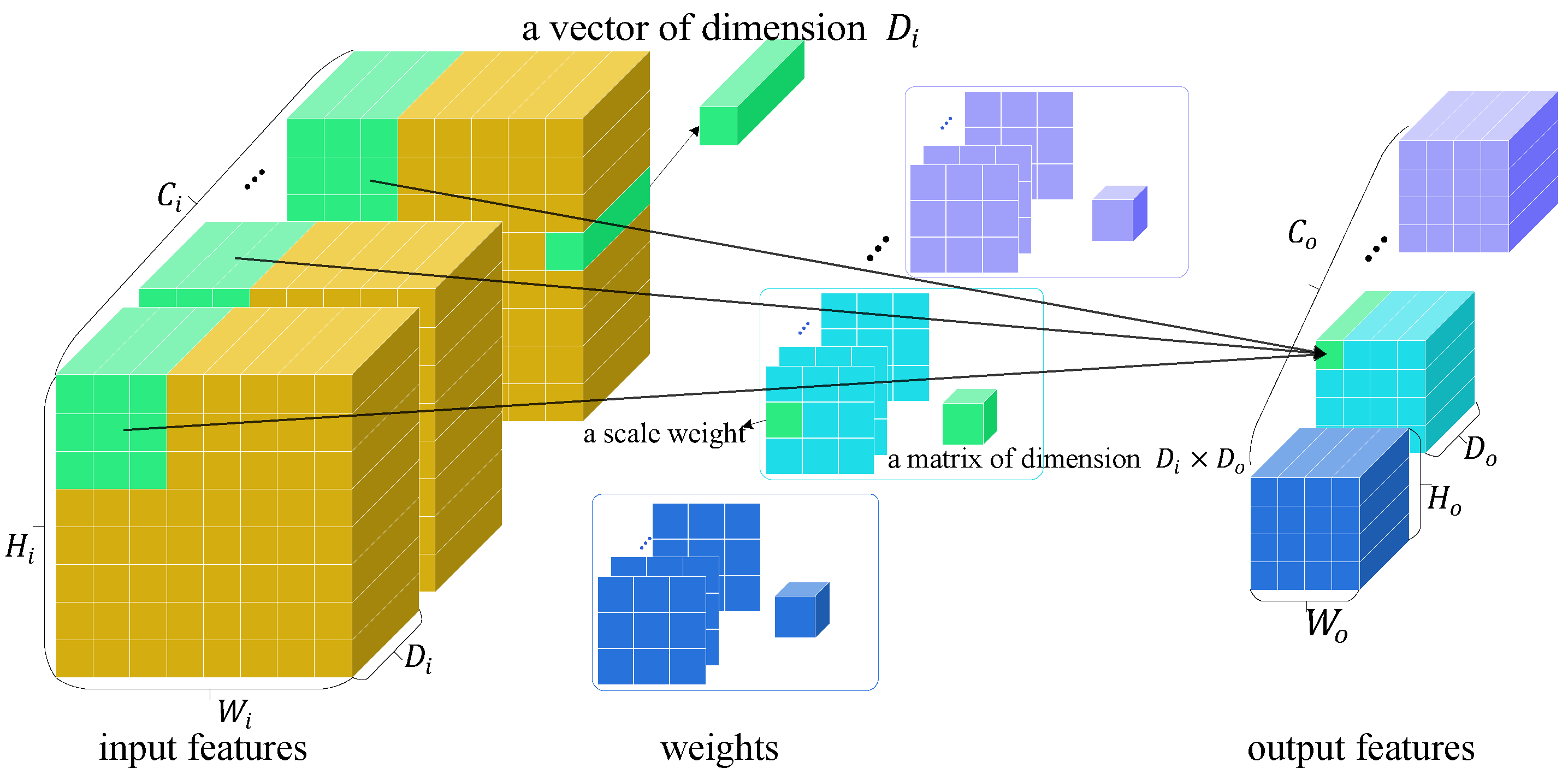
• $D_i,D_o$: dimensionality of input/output vexels
• $r,s$: indices of input/output channels
• $p,q$: spatial indices in the input
• $h,w$: spatial indices in the output
• $\mathrm{MatMul}(A,B)$: matrix–vector multiplication
• $a·\mathbf{v}$: scalar–vector product

Unless stated otherwise, we use superscripts for channel or receptive field indices and subscripts for spatial positions within feature maps.

4.2. Adaptive and Biased Mixed Weights

Differing from Dynamic Routing [23] and EM Routing [28], we design a simpler and lighter-weight mechanism for vexels passing information, simultaneously adopting adaptive weights and biased weights. Hahn et al. [21] consider routing mechanisms in CapsNets to be a specific type of Mixture of Experts; they adopt a simple linear layer to act as the Mixture of Experts’ routing, replacing Dynamic routing [23] and EM routing [28] in CapsNet. In the convolutional version of SR-Capsule Nets, Hahn et al. use a distinct $C_o\times D_i$ matrix to compute a scalar coefficient for controlling the contribution of each input capsule to each output capsule.

To make the routing process more robust and less computation intensive, we propose to average all the components of each input vexel first and then let a $C_o\times 1$ matrix map the input vexel’s mean to the contribution coefficient between itself and the output vexels. Considering the receptive field and channels, we give the process of computing coefficients in Equation (4). At the same time, we do not represent activations with additional tensors but denote activations by vexels norms. Experiments show that these modifications bring better prediction and computation performance. Note that the weights made up by these controlling coefficients apply to input vexel features in a scalar way, thus we denote these weights with a tensor named $\mathbf{S}$. It is not hard to observe that $\mathbf{S}$ is adaptive because it is dynamically calculated based on input vexel features, making up the A weights in our algorithm.

$$\begin{array}{c}\hfill \left\{\begin{array}{cc}\hfill {\overline{\mathbf{U}}}_{p,q}^r& ={\displaystyle \frac{1}{D_i}}\sum _{n=0}^{D_i}{\mathbf{U}}_{p,q}^r\left(n\right)\hfill \\ \hfill {\mathbf{S}}_{p,q}^{s,r}& ={\overline{\mathbf{R}}}_{p,q}^s·{\mathbf{W}}^{\mathbf{S}}{s,r}_{p,q}\hfill \end{array}\right.\end{array}$$

(4)

where $\mathbf{U}\in {\mathbb{R}}^{C_i\times H_i\times W_i\times D_i}$ and $\overline{\mathbf{U}}\in {\mathbb{R}}^{C_i\times H_i\times W_i}$ denote input vexel features and the mean averaged from each vexel, respectively, $\mathbf{S}$ and ${\mathbf{W}}^{\mathbf{S}}\in {\mathbb{R}}^{C_o\times C_i\times H_k\times W_k}$ indicate the mapping for computing the contribution coefficients and the computed coefficients, respectively, while $\mathbf{R}$ stands for the receptive field in input vexel features, which is an area with the same shape as the convolutional kernel weights. Finally, ${\overline{\mathbf{R}}}_{p,q}^s$ is a receptive field on ${\overline{\mathbf{U}}}_{p,q}^r$ centered at position $(p,q)$.

The part B weights are the matrix coefficients applied on vexels through matrix multiplication; we denote them by B since they are predefined in the beginning and are then updated during training; in other words, they are bias weights. To share bias weights to varying extents, we design different operators for B’s computation in the following.

Overall, we provide Algorithms 1 and 2, which present the fundamental procedures of vexel operators. Firstly, in Algorithm 1, we compute adaptive weights from input vexels and predefined bias weights, using vexels’ means and norms. We give the formula of in-place softmax [32] as follows for easy understanding:

$$u_{i,j}={\displaystyle \frac{e^{u_{i,j}}}{{\sum }_{j=0}^{D_i}{e}^{u_{i,j}}}}$$

(5)

Combining the calculated adaptive scalar weights and predefined bias matrix weights, we obtain the output vexels in Algorithm 2.

Algorithm 1 Vexel voting algorithm

Input: features $\mathbf{U}\in {\mathbb{R}}^{N_i\times D_i}$ coefficient, weights ${\mathbf{W}}^{\mathrm{S}}\in {\mathbb{R}}^{N_o\times N_i}$. Output: adaptive scalar weights $\mathbf{S}\in {\mathbb{R}}^{N_o\times N_i}$. ▹$N_i=C_i\times H_k\times W_k$, $N_o=C_o\times H_o\times W_o$. 1: procedure Compute means and norms of input vexels 2:     for ${\mathbf{u}}_n\in {\mathbb{R}}^{D_i}$ traverse in $\mathbf{U}$ do, $$\begin{array}{c}{\overline{u}}_n={\displaystyle \frac{1}{D_i}}\sum _{j=0}^{D_i-1}{u}_{i,j}\\ a_n=\sqrt{\sum _{j=0}^{D_i-1}{u}_{i,j}^2}\end{array}$$ (6) 3:     end for 4:     All ${\overline{u}}_n$ form $\overline{\mathbf{U}}\in {\mathbb{R}}^{N_i}$, and all $a_n$ form $\mathbf{A}\in {\mathbb{R}}^{N_i}$ 5: end procedure 6: procedure Compute adaptive scalar weights $\mathbf{S}\in {\mathbb{R}}^{N_o\times N_i}$ 7:     for ${\overline{u}}_n$ traverse in $\overline{\mathbf{U}}$, and ${\mathbf{w}}_n^{\mathrm{S}}\in {\mathbb{R}}^{N_o}$ traverse in ${\mathbf{W}}^{\mathrm{S}}$ do; $${\mathbf{s}}_n={\overline{u}}_n\ast {\mathbf{w}}_n^{\mathrm{S}}$$ (7) 8:     end for 9:     All ${\mathbf{s}}_n$ form Adaptive coefficients $\mathbf{S}$. 10:     Apply softmax Equation (5) along $N_o$ dimension upon $\mathbf{S}$. $$\mathbf{S}=\underset{N_o}{\mathrm{Softmax}}\left(\mathbf{S}\right).$$ (8) 11: end procedure 12: procedure Compute voting coefficients. 13:     for ${\overline{a}}_n$ traverse in $\mathbf{A}$, ${\mathbf{s}}_n$ traverse in $\mathbf{S}$ do; $${\mathbf{r}}_n={\overline{a}}_n\ast {\mathbf{s}}_n$$ (9) 14:     end for 15:     all ${\mathbf{r}}_n$ form voting coefficients $\mathbf{R}\in {\mathbb{R}}^{N_o\times N_i}$. 16:     normalize $\mathbf{R}$ via, $${\mathbf{R}}_{i,j}={\displaystyle \frac{1}{{\sum }_{j=1}^{N_i}{\mathbf{R}}_{i,j}}}{\mathbf{R}}_{i,j}$$ (10) 17: end procedure

Algorithm 2 Vexel propagation algorithm

Input: features $\mathbf{U}\in {\mathbb{R}}^{N_i\times D_i}$, bias matrix weights ${\mathbf{W}}^{\mathrm{M}}\in {\mathbb{R}}^{N_o\times N_i\times D_i\times D_o}$, coefficient weights ${\mathbf{W}}^{\mathrm{S}}\in {\mathbb{R}}^{N_o\times N_i}$. Output: features $\mathbf{V}\in {\mathbb{R}}^{N_o\times D_o}$. ▹ Note that for convolution, $N_i=C_i\times H_k\times W_k$, $N_o=C_o\times H_o\times W_o$. 1: Compute Adaptive scalar weights $\mathbf{R}\in {\mathbb{R}}^{N_o\times N_i}$ by Algorithm 1. 2: for $m=0$ to $N_o-1$ do; 3:     fetch ${\mathbf{u}}_n$ from $\mathbf{U}$ 4:     for $n=0$ to $N_i-1$ do; 5:         fetch ${\mathbf{w}}_{m,n}^{\mathrm{M}}\in {\mathbb{R}}^{D_i\times D_o}$ from ${\mathbf{W}}^{\mathrm{M}}$, and scalar $r_{m,n}$ from $\mathbf{R}$. 6:         compute quasi vexel ${\overline{\mathbf{u}}}_{m,n}\in {\mathbb{R}}^{D_o}$ via, $${\overline{\mathbf{u}}}_{m,n}=r_{m,n}·\mathrm{MatMul}({\mathbf{u}}_n,{\mathbf{w}}_{m,n}^{\mathrm{M}}),$$ (11) 7:     end for 8:     get mth output vexel ${\mathbf{v}}_m\in {\mathbb{R}}^{D_o}$ via summing ${\overline{\mathbf{u}}}_{m,n}$ along $N_i$, $${\mathbf{v}}_m=\sum _{n=0}^{N_i-1}{\overline{\mathbf{v}}}_{m,n}$$ (12) 9: end for 10: all ${\mathbf{v}}_m$ form output vexels $\mathbf{V}\in {\mathbb{R}}^{N_o\times D_o}$.

4.3. Vexel Operators

In this part, we introduce different vexel operators. We reshape the features from CNNs into vexel features by grouping the channels into several segments; thus, we can implement a convolution-style operator on vexel features, as in [21,28].

Vexel-wised operator. The vexel-wise operator slides on vexel feature maps, as shown in Figure 3. Let $\mathbf{M}\in {\mathbb{R}}^{C_o\times C_i\times H_k\times W_k\times D_i\times D_o}$ denote the aforementioned B weights. Compared with CNNs’ weights, our vexel operator replaces every scalar value in the kernel with a matrix of dimension $D_i\times D_o$, multiplying them with vexel vectors. Moreover, each multiplication result is weighted with learned voting coefficients.

For friendly comprehension, we show the calculation of a vexel located at $(h,w)$ in the sth channel output features ${\mathbf{V}}^s$ by Equation (13). At sliding step $stride$, ${\mathbf{M}}^s$, i.e., the bias matrix weights corresponding to calculating the sth channel output features, covers a region across all channels on input features $\mathbf{U}$ centered at position $(h·stride,w·stride)$, i.e., the receptive field, conveniently denoted as ${\mathbf{R}}^{(h,w)}\in {\mathbb{R}}^{C_i\times H_k\times W_k}$, the height, width, and channels of which equal to those of ${\mathbf{M}}^s$ separately. Then, every vexel in ${\mathbf{R}}^{(h,w)}$ is affinely transformed by the corresponding matrix in $\mathbf{A}$ through matrix multiplication.

$${\mathbf{V}}_{h,w}^s=\sum _{r=0}^{C_i}\sum _{p=0}^{H_k}\sum _{q=0}^{W_k}\mathrm{MatMul}({{\mathbf{R}}^{(h,w)}}_{p,q}^r·{\mathbf{S}}_{p,q}^{s,r},{\mathbf{M}}_{p,q}^{s,r})$$

(13)

where ${{\mathbf{R}}^{(h,w)}}_{p,q}^r,{\mathbf{M}}_{p,q}^{s,r}$ are a matrix and a vector, respectively, · indicates scalar multiplication and $\mathrm{MatMul}(,)$ refers to the matrix multiplication operator. Note that both $\mathbf{R}$ and ${\mathbf{M}}^s$ consist of $C_{in}$ channels. All the output features are obtained after $C_s$ different ${\mathbf{M}}^s$’s have slid on the whole $\mathbf{U}$.

Channel-wise operator. The vexel-wise operator introduced above is naive; although weights are shared across the spatial dimensions of input, they are still heavily parameterized. To balance the trade-off between weight burden and generalization ability, we design a channel-wise operator, which further shares matrix weights within the receptive field, resulting in lighter $\mathbf{M}\in {\mathbb{R}}^{C_o\times C_i\times D_i\times D_o}$, as shown in Figure 4.

The calculation of output vexel ${\mathbf{V}}^{(i,j)}$ at position $(i,j)$ in feature map $\mathbf{V}$ involves few parameters, as shown in Figure 4 and Equation (14).

$${\mathbf{V}}_{h,w}^s=\sum _{r=0}^{C_i}\mathrm{MatMul}(\sum _{p=0}^{H_k}\sum _{q=0}^{W_k}{{\mathbf{R}}^{(h,w)}}_{p,q}^r·{\mathbf{S}}_{p,q}^{s,r},{\mathbf{M}}^{s,r})$$

(14)

where, ${\mathbf{S}}_{p,q}^{s,r}$ is a scale parameter, while ${\mathbf{M}}_p^s$ is a matrix of shape $D_i\times D_o$.

All-channel operator. To reduce the number of parameters, we design a vexel operator sharing matrix weights among the receptive field, as presented in Figure 5. In this situation, the calculation of ${\mathbf{V}}^{(i,j)}$ is formulated as Equation (15).

$${\mathbf{V}}_{h,w}^s=\mathrm{MatMul}(\sum _{r=0}^{C_i}\sum _{p=0}^{H_k}\sum _{q=0}^{W_k}{{\mathbf{R}}^{(h,w)}}_{p,q}^r·{\mathbf{S}}_{p,q}^{s,r},{\mathbf{M}}^s)$$

(15)

where $\mathbf{M}\in {\mathbb{R}}^{C_o\times D_i\times D_o}$ contains fewer parameters, and ${\mathbf{M}}^o$ is a $D_i\times D_o$ matrix.

Cyclic operator. Models that are too lightweight often lack generalization ability, i.e., these models cannot always extract appropriate features for various recognition tasks and data. To remedy the possible insufficient learning capability of the above two convolutional operators that share bias matrix weights, we devise the cyclic vexel operator, shown in Figure 6; it contains few parameters and at the same time, it maintains appreciable learning capacity. Based on the mechanism of the channel-wise operator, for a $D_i$-dimensional vexel $r_{p,q}={{\mathbf{R}}^{(h,w)}}_{p,q}^r$ in receptive field ${\mathbf{R}}^{(h,w)}$, there are two cases for its location, the center of ${\mathbf{R}}^{(h,w)}$ or elsewhere. Thus, we apply a shared matrix on $r_{p,q}$ if it is at the center. Otherwise, we use another one.

$$\begin{array}{cc}\hfill {\mathbf{V}}_{h,w}^s=\sum _{r=0}^{C_i}& \mathrm{MatMul}(\sum _{p\ne {\displaystyle \frac{H_k}{2}}}\sum _{q\ne {\displaystyle \frac{W_k}{2}}}{{\mathbf{R}}^{(h,w)}}_{p,q}^r{\mathbf{S}}_{p,q}^{s,r},{\mathbf{M}}_0^{s,r})\hfill \\ \hfill & +\mathrm{MatMul}({{\mathbf{R}}^{(h,w)}}_{{\displaystyle \frac{H_k}{2}},{\displaystyle \frac{W_k}{2}}}^r{\mathbf{S}}_{{\displaystyle \frac{H_k}{2}},{\displaystyle \frac{W_k}{2}}}^{s,r},{\mathbf{M}}_1^{s,r})\hfill \end{array}$$

(16)

where we can see that the shape of $\mathbf{M}$ in this situation is ${\mathbb{R}}^{C_o\times C_i\times 2\times D_i\times D_o}$.

4.4. Relation to CapsNets

Pose and activation. Capsules and vexels both extract features into poses, which indicate the relative transformations between observer’s coordinate frame and the world’s coordinate frame; therefore, they both try to represent objects as spatial relationships between the object’s parts and the whole object. As for activation values, which are necessary for artificial neural networks imitating the mechanism of the human neural system, in [23], the activation of a capsule is denoted by its norm. At the same time, in [20,21,28], a separate scalar is introduced to represent the activation for a capsule, relatively decoupling the routings of activation values and poses. After comparing the prediction performance, we determined activation values by their norms.

Squash function. As we represented the activation value of a vexel by its norm, we adopted the squash function from [23]. As mentioned by Hinton et al., that function can let norms of vexels be scaled and split so that norms of too-short vexels approximate 0, the norms of too-long vexels are pulled towards 1, and the norms of other vexels are squashed between 0 to 1.

$${\mathbf{v}}_j={\displaystyle \frac{{\parallel {\mathbf{v}}_j\parallel }^2}{1+{\parallel {\mathbf{v}}_j\parallel }^2}}{\displaystyle \frac{{\mathbf{v}}_j}{\parallel {\mathbf{v}}_j\parallel }}$$

(17)

Marginal loss. Matching the squash function, the marginal loss $l_k$ is calculated for each target class k in recognition for measuring the discrepancy between the predicted class and the ground-truth class. We set $\lambda =0.5$ and $m^{+}=0.9,m^{-}=0.1$, as in [23]. We tested other loss functions, such as NLL and CrossEntropy on CIFAR-10, and observed lower accuracy compared to the marginal loss. As shown in

Table 2. Comparison of different loss functions (NLL, CrossEntropy, and marginal loss) on CIFAR-10. The results demonstrate that the marginal loss is more compatible with the squash function, achieving the highest accuracy among the compared loss functions.

Loss Function	Accuracy (%)
Marginal loss	92.52
NLL loss	91.51
CrossEntropy Loss	92.47

, the marginal loss outperformed both NLL and CrossEntropy, demonstrating its better alignment with the squash function and superior performance in our method.

$$\begin{array}{cc}\hfill l_k=& T_{k}max(0,m^{+}-\parallel {\mathbf{v}}_k{\parallel )}^2+\hfill \\ \hfill & \lambda (1-T_k)max(0,\parallel {\mathbf{v}}_k{\parallel -m^{-})}^2\hfill \end{array}$$

(18)

Cyclic self-routing. We also utilized our cyclic-styled computation mechanism in Self-Routing Capsule [21], denoted by CyclicSR, by which we reduced the number of matrices from the size of the receptive field to 2, similar to how it was performed for cyclic vexel convolution. Moreover, we validate and compare it with the aforementioned vexel operators in Section 5.5.

5. Results

In this section, we present the results showing the effectiveness of our method and compare its performance with state-of-the-art CapsNets [20,21,23,28,33]. Rather than focusing solely on classification accuracy on standard benchmarks, we systematically evaluated the balancing between computation overhead and generalizability of VexNets by varying its vexel operators. We also assessed the robustness of different methods via adversarial-attack experiments and affine-transformation tests. Furthermore, we conducted ablation studies to highlight the advantages of our proposed approach. For a fair comparison, we also report the results of CNN-based baselines from [21], where “AvgPool” and “Conv” denote architectures in which average-pooling and convolutional layers replace the capsule and vexel layers, respectively.

5.1. Implementation Details

Datasets. We evaluated all methods on four standard benchmarks, FashionMNIST [34], SVHN [35], CIFAR-10 [36], and smallNORB [37], which are briefly described as follows:

• FashionMNIST comprises 60,000 training and 10,000 test grayscale images of size $28\times 28$, spanning 10 fashion categories.
• SVHN contains 73,257 training and 26,032 test RGB images of size $32\times 32$, depicting house numbers.
• CIFAR-10 consists of 50,000 training and 10,000 test RGB images of size $32\times 32$, covering 10 object classes.
• smallNORB is a 3D object recognition dataset with $96\times 96$ grayscale images of five object categories, captured under varying lighting, azimuth, and elevation conditions.

Training configurations. All experiments were conducted on an Intel Xeon Gold 5220 CPU and four NVIDIA Tesla A40 GPUs. To ensure a fair comparison, each model was trained for 350 epochs on CIFAR-10, 200 on SVHN, and 100 on smallNORB. We set the initial learning rate to 0.1 and decayed it by a factor of 10 at epochs 150 and 250 for CIFAR-10, 100 and 150 for SVHN, and 50 and 75 for smallNORB. Optimization was performed using stochastic gradient descent (SGD) [11] with the distinct loss functions specified in the respective papers. Each dataset was divided into training, validation, and test sets. We trained each method on the training split (using the validation split for model selection) and report its classification accuracy on the test split. Model parameter counts and FLOPs were computed using the calflops library [38].

Evaluation metrics. We used classification accuracy to quantify performance on all image classification tasks. To visualize the classification efficiency, we present Receiver Operating Characteristic (ROC) curves [39], confusion matrices [40], and t-SNE visualizations [41] in Section 5.3 for each method.

Network architectures. All methods shared a common CNN backbone with distinct task-specific heads. Backbone architectures varied by dataset, except for the Variational Bayes CapsNet [20], which strictly followed the original implementation. Specifically,

• For CIFAR-10 and SVHN: 19 convolutional layers organized into eight residual blocks;
• For smallNORB: six convolutional layers;
• For FashionMNIST and affineMNIST: a single convolutional layer.

All method-specific heads used identical hyperparameter settings. Detailed architectures for the ablation studies are given in Section 5.5.

Code implementation. Our experiment was implemented in Python 3.10 using PyTorch 2.0.1 [42], PyTorch Lightning 2.1.0 [43], and CUDA 11.8 [44]. Performance-sensitive operators for VexNet were implemented in C++ [45] and compiled with the GNU Compiler Collection (GCC) [46]. The complete codebase is available at https://github.com/onbigion13/VexNet (accessed on 22 September 2024).

Notation.

Table 3. Abbreviations and corresponding methods.

Abbreviation	Method
CapsNets
DR	Dynamic Routing CapsNet [23]
EM	EM Routing CapsNet [28]
SR	Self-Routing CapsNet [21]
VB	Variational Bayes CapsNet [20]
ResRouting	Residual Dynamic Routing [33]
VexNets
Vex-VW	VexNet with vexel-wise operator
Vex-CW	VexNet with channel-wise operator
Vex-AC	VexNet with all-channel operator
Vex-Cyclic	VexNet with cyclic vexel operator
Vex-CyclicSR	VexNet with self-routing

summarizes the abbreviations used throughout this part.

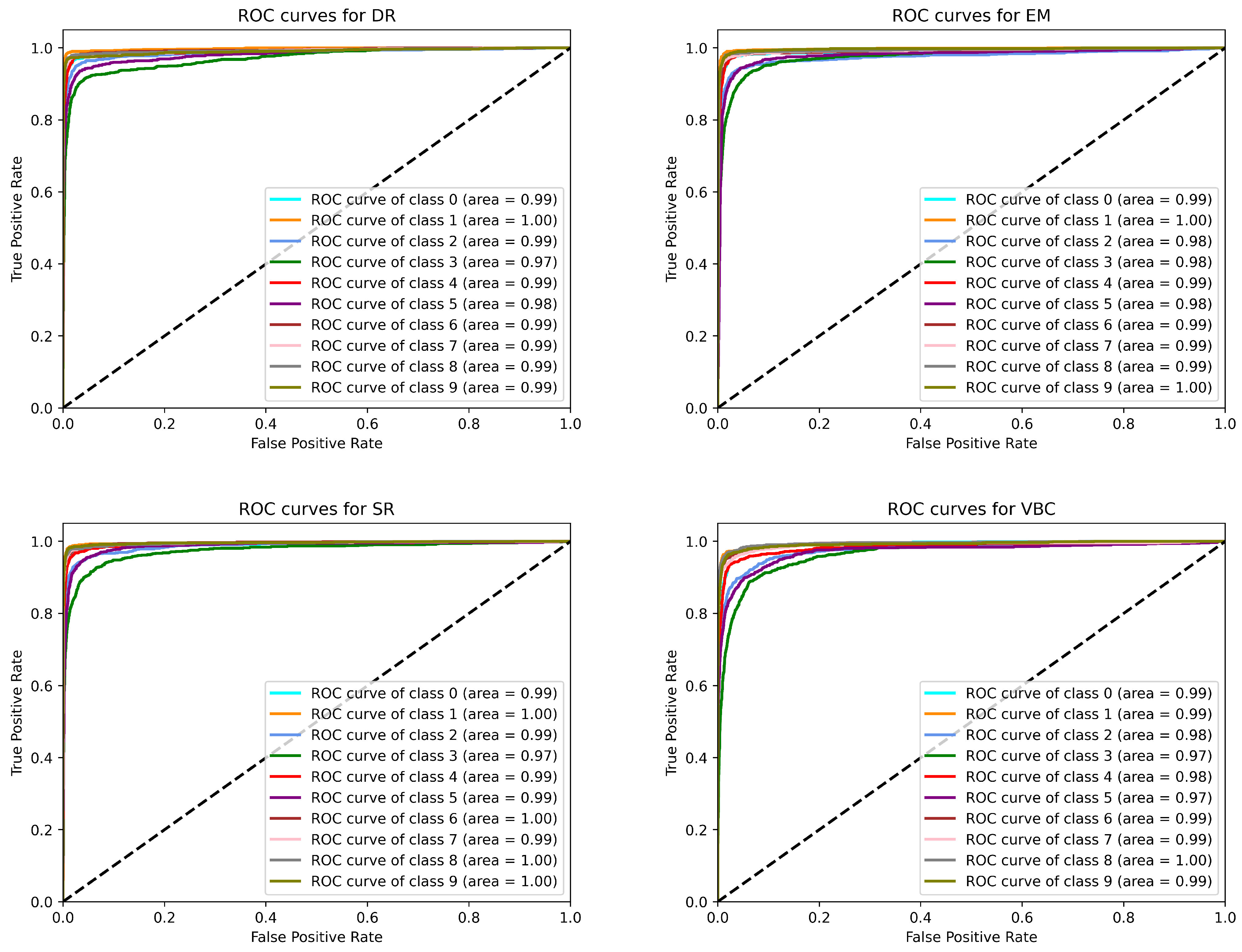
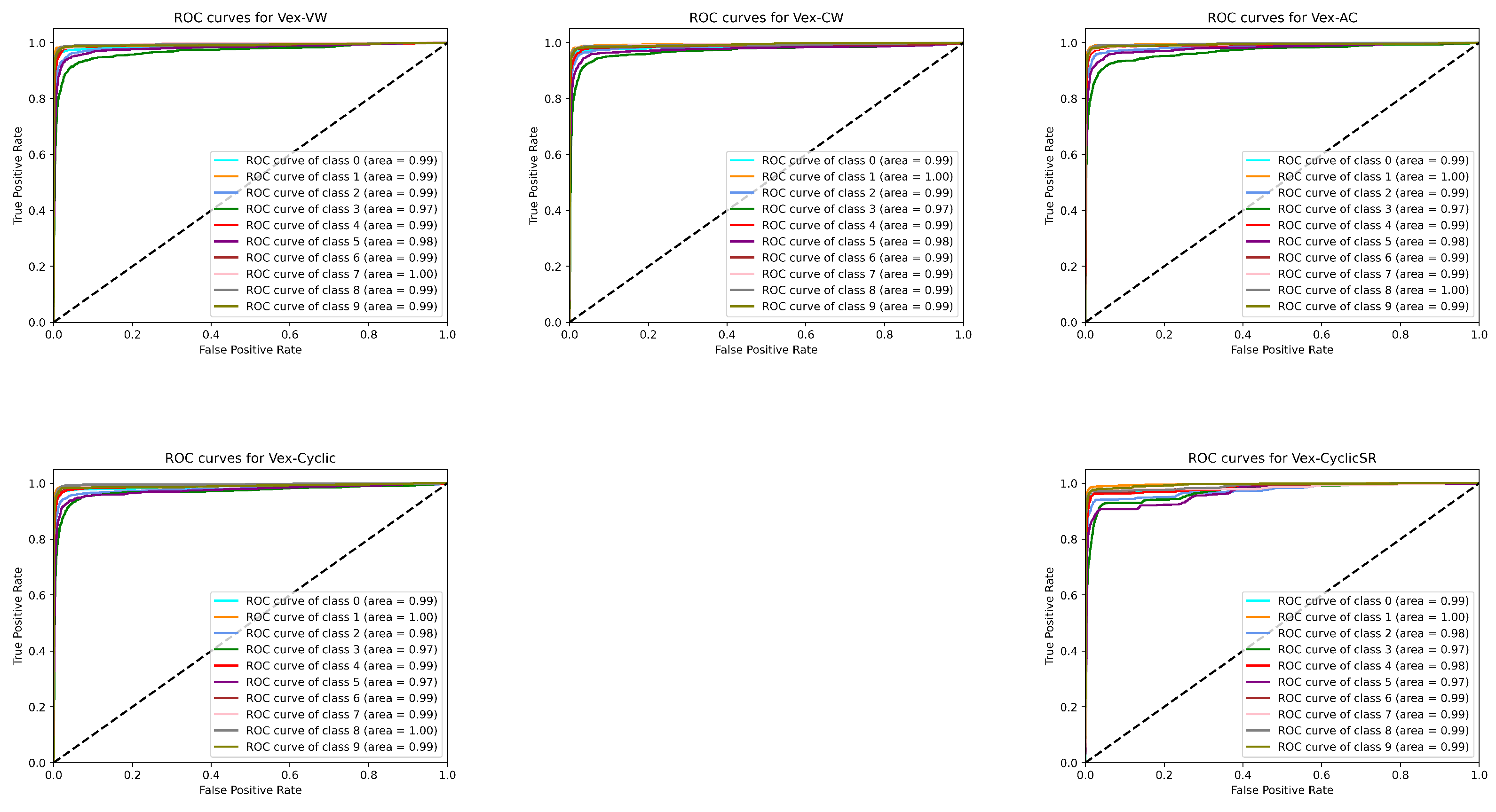
5.2. Image Classification Results

As shown in

Table 4. Image classification accuracies on CIFAR-10 and SVHN.

Methods	CIFAR-10 (%)	SVHN (%)	Params (M)	FLOPs (M)
Vex-VW	92.48	96.40	2.60	91.41
Vex-CW	92.47	96.44	1.37	88.95
Vex-AC	92.52	96.39	1.29	88.79
Vex-Cyclic	92.44	96.40	1.45	89.03
DR [23]	92.21	96.33	2.59	91.23
EM [28]	91.46	95.78	1.40	89.86
SR [21]	92.31	96.12	1.40	89.96
VB [20]	88.49	94.80	0.32	38.27
ResRouting [33]	92.38	96.16	1.40	89.86
AvgPool	92.06	96.45	0.30	41.30
Conv	89.99	96.02	0.90	61.00

, VexNets consistently outperformed CapsNet baselines on both CIFAR-10 and SVHN. Notably, Vex-AC achieved 92.52% on CIFAR-10, surpassing Dynamic Routing CapsNet by 0.31 points (92.21%) while using only 1.29 M parameters (vs. 2.59 M) and 88.79 M FLOPs (vs. 91.23 M). On SVHN, Vex-CW attained 96.44%, outperforming EM Routing CapsNet by 0.66 points (95.78%) with 1.37 M parameters compared to 1.40 M. Even the most compact VexNet model (Vex-AC) maintained state-of-the-art accuracy with substantially fewer resources, demonstrating the efficiency of our adaptive weight and MoE subnetworks in Self-Routing CapsNet [21].

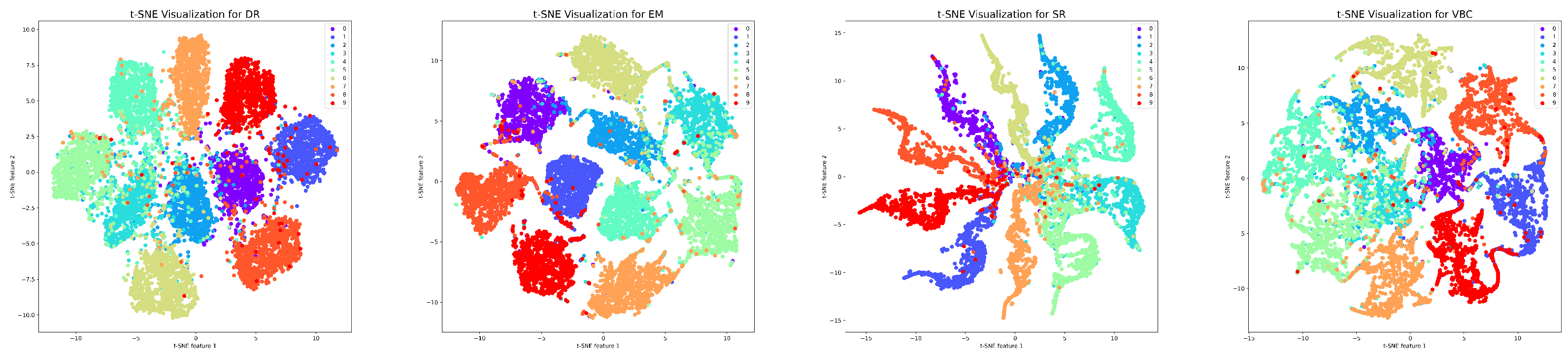
5.3. Visualization of Classification

To qualitatively assess classification performance, we plotted Receiver Operating Characteristic (ROC) curves, confusion matrices, and t-SNE embeddings for all methods.

ROC curves. Figure 7 and Figure 8 show the ROC curves for CapsNets and VexNets, respectively.

Table 5. Average per-class AUC on CIFAR-10 (mean over 10 classes).

Capsule Networks
DR	0.988
EM	0.989
SR	0.992
VB	0.985
VexNets
Vex-VW	0.988
Vex-CW	0.988
VEx-AC	0.989
Vex-Cyclic	0.987
Vex-CyclicSR	0.985

reports the average per-class Area Under the ROC Curve (AUC) on CIFAR-10—higher AUC indicates better class separability. VexNet with all channel-shared kernel operators achieved 0.989 average AUC, surpassing Dynamic Routing CapsNet (0.988) and Variational Bayes CapsNet (0.985) and matching EM Routing CapsNet (0.989). The vexel-wise and channel-wise variants reached 0.988, outperforming Variational Bayes and equaling Dynamic Routing. Self-Routing CapsNet led with 0.992 among the baselines, while Variational Bayes CapsNet had the lowest AUC (0.985). When considered alongside substantially fewer parameters and FLOPs (see Table 4), these results demonstrate that VexNets deliver competitive or superior discriminative performance with greater computational efficiency.

Confusion matrices. Figure 9 and Figure 10 show the confusion matrices for capsule networks and VexNets, respectively. Each confusion matrix illustrates the matching between predicted and true labels, with larger diagonal values indicating more accurate predictions. Compared to their CapsNet counterparts, VexNet variants consistently exhibited higher diagonal entries, indicating improved class discrimination and more accurate label assignment.

t-SNE Embeddings. t-SNE is a dimensionality reduction technique that projects high-dimensional data into a low-dimensional space to visualize the feature distributions. A good t-SNE visualization exhibits distinct, well-separated clusters related to each category, with minimal overlap. As shown in Figure 11 and Figure 12, CapsNets generally produced clustered features; however, many feature points intruded into regions of other classes, particularly for Dynamic Routing CapsNet and Variational Bayes CapsNet, where inter-class mixing became pronounced. By contrast, VexNet variants consistently achieved better feature separation: although some intermingling still existed, features from different categories formed compact clusters and exhibited more precise boundaries between groups.

5.4. Robustness Experiments

We evaluated the robustness of VexNets and CapsNets against both affine viewpoint changes and adversarial attacks. Results are summarized in

Table 6. Classification accuracy (%) on smallNORB under affine transformations.

Method	Elevation Familiar	Novel	Azimuth Familiar	Novel
Vex-VW	94.85	83.83	93.20	81.94
Vex-CW	95.15	81.78	93.60	81.72
Vex-RW	95.22	82.11	92.86	81.67
Vex-Cyclic	95.61	82.51	93.44	81.60
DR	94.50	81.90	92.67	80.85
EM	93.84	80.64	92.94	80.65
SR	94.25	82.74	92.85	81.67
AvgPool	94.32	82.28	91.51	78.24
Conv	92.49	81.22	91.61	77.93

,

Table 7. Attack success rates (%) under FGSM adversarial attacks.

	CIFAR-10		SVHN
	Targeted	Untargeted	Targeted	Untargeted
Vex-VW	4.39	15.62	2.77	21.82
Vex-CW	4.15	14.93	2.35	12.04
Vex-RW	4.37	20.32	2.78	15.68
Vex-Cyclic	5.51	24.75	2.71	24.69
DR [23]	6.33	39.76	2.93	20.50
EM [28]	9.85	45.94	7.65	33.61
SR [21]	5.36	37.64	4.93	25.53
AvgPool	18.46	62.65	15.38	44.44
Conv	21.61	60.57	17.94	44.47

and

Table 8. Attack success rates (%) under BIM adversarial attacks.

	CIFAR-10		SVHN
	Targeted	Untargeted	Targeted	Untargeted
Vex-VW	15.75	14.79	8.45	22.75
Vex-CW	8.90	12.13	6.89	8.88
Vex-RW	11.41	14.63	9.50	11.40
Vex-Cyclic	13.57	20.70	9.79	15.41
DR [23]	15.36	45.47	8.83	30.63
EM [28]	36.57	66.74	20.87	44.62
SR [21]	17.61	55.96	14.82	37.58
AvgPool	45.40	84.90	42.60	62.20
Conv	42.80	82.00	41.80	62.60

. Results for Variational Bayes CapsNet (VB) [20] are not reported here, as it exhibited consistently poor resistance to affine transformations and adversarial attacks, and its inference process was significantly slower than that of competing methods.

5.4.1. Robustness to Affine Transformation

We assessed accuracy on smallNORB under familiar viewpoints (azimuths/elevations seen during training) and novel viewpoints (unseen combinations). Table 6 reports these results. VexNet variants consistently outperformed CapsNets, especially under novel conditions. For example, VexNet with the vexel-wise operator achieved 83.83% on novel elevations—1.09 points higher than Self-Routing CapsNet (82.74%)—and VexNet with the cyclic operator reached 93.44% on familiar azimuths versus 92.94% for EM Routing CapsNet.

5.4.2. Robustness to Adversarial Attack

Adversarial attacks craft small, imperceptible perturbations to input images to cause neural networks to make incorrect predictions. Untargeted attacks seek to cause any incorrect prediction, whereas targeted attacks force the model to classify inputs as a specified wrong class. Lower attack success rates indicate stronger model robustness against such perturbations. We generate adversarial examples using FGSM [47] and BIM [18] and report attack success rates (lower is better) on CIFAR-10 and SVHN. VexNet with channel-wise operator achieved the lowest success rates across both datasets and attack types. For instance, against FGSM and BIM attacks, VexNet with the channel-wise operator consistently achieved the lowest success rates (e.g., 12.13% vs. 45.47% for Dynamic Routing under untargeted BIM on CIFAR-10), demonstrating superior adversarial resilience.

5.5. Ablation

We performed an ablation study on CIFAR-10 to evaluate the impact of different vexel operators and architectural configurations. Using the backbone from Section 5.2, each variant was trained for five independent runs. Unlike Section 5.2, we selected the model at the final validation epoch for testing here.

Table 9. Ablation results on CIFAR-10 (accuracy ± std %).

	Vex-VW	Vex-CW	Vex-RW	Vex-Cyclic	Vex-CyclicSR
${32}^C\times {16}_D$, Vex-1	92.33 ± 0.23	92.33 ± 0.12	92.20 ± 0.18	92.23 ± 0.29	91.93 ± 0.10
${32}^C\times {16}_D$, Vex-2	92.20 ± 0.16	92.22 ± 0.10	92.54 ± 0.24	92.30 ± 0.26	91.70 ± 0.47
${32}^C\times 8_D$, Vex-1	92.25 ± 0.26	92.12 ± 0.11	92.02 ± 0.22	92.21 ± 0.20	91.85 ± 0.15
${32}^C\times {32}_D$, Vex-1	92.25 ± 0.15	92.30 ± 0.16	92.22 ± 0.27	92.13 ± 0.19	91.63 ± 0.34
${16}^C\times {16}_D$, Vex-1	92.06 ± 0.14	92.20 ± 0.12	92.14 ± 0.10	92.33 ± 0.20	91.89 ± 0.16
${64}^C\times {16}_D$, Vex-1	92.17 ± 0.23	92.32 ± 0.12	92.34 ± 0.14	92.22 ± 0.35	91.92 ± 0.20

reports the mean test accuracy (±standard deviation) across runs.

The ablation results confirmed our theoretical predictions (Section 4.3). Under the ${32}^C\times {16}_D$, Vex-1 configuration, VexNet with vexel-wise and channel-wise operators both achieved 92.33% accuracy. In contrast, Vex-Cyclic dropped to 92.23% and Vex-CyclicSR further decreased to 91.93%, demonstrating that the cyclic operator’s additional weight sharing reduced performance and that combining it with self-routing did not offset that loss. Moreover, increasing the feature dimension in Vex-VW from 8 to 16 raised accuracy from 92.25% to 92.33%, and stacking two vexel layers in Vex-RW boosted performance to 92.54%, confirming that greater model capacity enhances recognition ability.

6. Conclusions

In this research, we introduced the concept of vexel, a novel feature representation that models features as vector-based maps. To effectively process vexel-based features, we proposed a specialized algorithm and four key computational operators, culminating in developing VexNet. VexNet achieved improved recognition robustness compared to capsule-based methods, significantly reducing model size and computational complexity. Extensive experiments across multiple benchmarks validated the effectiveness of the proposed method, demonstrating superior performance in image classification tasks, resilience to affine transformations, and robustness against adversarial attacks. Our ablation studies further highlighted the advantages of vexel-based representations in capturing spatial relationships and enhancing feature expressiveness. For future work, we plan to optimize vexel representations and extend their applicability to Multi-Layer Perceptrons (MLPs) and Recurrent Neural Networks (RNNs). Additionally, we aim to explore VexNet’s potential in broader application domains, including computer graphics, natural language processing (NLP), and reinforcement learning. We encourage the research community to contribute to refining and expanding vexel-based methodologies, driving further advances in representation learning.

References

1. Krizhevsky, A.; Sutskever, I.; Hinton, G.E. Imagenet classification with deep convolutional neural networks. Commun. ACM 2017, 60, 84–90. [Google Scholar] [CrossRef]
2. Graves, A.; Graves, A. Long short-term memory. In Supervised Sequence Labelling with Recurrent Neural Networks; Springer: Berlin/Heidelberg, Germany, 2012; pp. 37–45. [Google Scholar]
3. Tran, D.; Bourdev, L.; Fergus, R.; Torresani, L.; Paluri, M. Learning spatiotemporal features with 3d convolutional networks. In Proceedings of the IEEE International Conference on Computer Vision (ICCV), Santiago, Chile, 7–13 December 2015; pp. 4489–4497. [Google Scholar]
4. Bordes, A.; Usunier, N.; Garcia-Duran, A.; Weston, J.; Yakhnenko, O. Translating embeddings for modeling multi-relational data. Adv. Neural Inf. Process. Syst. 2013, 26, 2787–2795. [Google Scholar]
5. Baltrušaitis, T.; Ahuja, C.; Morency, L.P. Multimodal machine learning: A survey and taxonomy. IEEE Trans. Pattern Anal. Mach. Intell. 2018, 41, 423–443. [Google Scholar] [CrossRef] [PubMed]
6. Russakovsky, O.; Deng, J.; Su, H.; Krause, J.; Satheesh, S.; Ma, S.; Huang, Z.; Karpathy, A.; Khosla, A.; Bernstein, M.; et al. Imagenet large scale visual recognition challenge. Int. J. Comput. Vis. 2015, 115, 211–252. [Google Scholar] [CrossRef]
7. Lin, T.Y.; Maire, M.; Belongie, S.; Bourdev, L.; Girshick, R.; Hays, J.; Perona, P.; Ramanan, D.; Zitnick, C.L.; Dollár, P. Microsoft COCO: Common Objects in Context. arXiv 2014, arXiv:1405.0312. [Google Scholar]
8. Rumelhart, D.E.; Hinton, G.E.; Williams, R.J. Learning representations by back-propagating errors. Nature 1986, 323, 533–536. [Google Scholar] [CrossRef]
9. Linnainmaa, S. The Representation of the Cumulative Rounding Error of an Algorithm as a Taylor Expansion of the Local Rounding Errors. Ph.D. Thesis, University Helsinki, Helsinki, Finland, 1970. Master’s Thesis (in Finnish). [Google Scholar]
10. LeCun, Y.; Boser, B.; Denker, J.S.; Henderson, D.; Howard, R.E.; Hubbard, W.; Jackel, L.D. Backpropagation applied to handwritten zip code recognition. Neural Comput. 1989, 1, 541–551. [Google Scholar] [CrossRef]
11. Robbins, H.; Monro, S. A stochastic approximation method. In The Annals of Mathematical Statistics; Institute of Mathematical Statistics: Hayward, CA, USA, 1951; pp. 400–407. [Google Scholar]
12. Kingma, D.P.; Ba, J. Adam: A method for stochastic optimization. arXiv 2014, arXiv:1412.6980. [Google Scholar]
13. Simonyan, K.; Zisserman, A. Very deep convolutional networks for large-scale image recognition. arXiv 2014, arXiv:1409.1556. [Google Scholar]
14. Szegedy, C.; Liu, W.; Jia, Y.; Sermanet, P.; Reed, S.; Anguelov, D.; Erhan, D.; Vanhoucke, V.; Rabinovich, A. Going deeper with convolutions. In Proceedings of the IEEE Conference on Computer Vision and Pattern Recognition, Boston, MA, USA, 7–12 June 2015; pp. 1–9. [Google Scholar]
15. He, K.; Zhang, X.; Ren, S.; Sun, J. Deep residual learning for image recognition. In Proceedings of the IEEE Conference on Computer Vision and Pattern Recognition, Las Vegas, NV, USA, 27–30 June 2016; pp. 770–778. [Google Scholar]
16. Szegedy, C.; Zaremba, W.; Sutskever, I.; Bruna, J.; Erhan, D.; Goodfellow, I.; Fergus, R. Intriguing properties of neural networks. arXiv 2013, arXiv:1312.6199. [Google Scholar]
17. Nguyen, A.; Yosinski, J.; Clune, J. Deep neural networks are easily fooled: High confidence predictions for unrecognizable images. In Proceedings of the IEEE Conference on Computer Vision and Pattern Recognition, Boston, MA, USA, 7–12 June 2015; pp. 427–436. [Google Scholar]
18. Kurakin, A.; Goodfellow, I.J.; Bengio, S. Adversarial examples in the physical world. In Artificial Intelligence Safety and Security; Chapman and Hall/CRC: Boca Raton, FL, USA, 2018; pp. 99–112. [Google Scholar]
19. Su, J.; Vargas, D.V.; Sakurai, K. One pixel attack for fooling deep neural networks. IEEE Trans. Evol. Comput. 2019, 23, 828–841. [Google Scholar] [CrossRef]
20. Ribeiro, F.D.S.; Leontidis, G.; Kollias, S. Capsule routing via variational bayes. In Proceedings of the AAAI Conference on Artificial Intelligence, New York, NY, USA, 7–12 February 2020; Volume 34, pp. 3749–3756. [Google Scholar]
21. Hahn, T.; Pyeon, M.; Kim, G. Self-routing capsule networks. In Proceedings of the Advances in Neural Information Processing Systems, Vancouver, BC, Canada, 8–14 December 2019; Volume 32. [Google Scholar]
22. Pechyonkin, M. Understanding Hinton’s Capsule Networks Part I: Intuition. 2017. Available online: https://medium.com/ai%C2%B3-theory-practice-business/understanding-hintons-capsule-networks-part-i-intuition-b4b559d1159b (accessed on 11 October 2023).
23. Sabour, S.; Frosst, N.; Hinton, G.E. Dynamic routing between capsules. arXiv 2017, arXiv:1710.09829. [Google Scholar]
24. Lenc, K.; Vedaldi, A. Understanding image representations by measuring their equivariance and equivalence. In Proceedings of the IEEE Conference on Computer Vision and Pattern Recognition, Boston, MA, USA, 7–12 June 2015; pp. 991–999. [Google Scholar]
25. Baeldung. Translation Invariance and Equivariance in Computer Vision. Online Forum Comment. 2022. Available online: https://www.baeldung.com/cs/translation-invariance-equivariance (accessed on 1 September 2023).
26. Duval, L. What Is the Difference Between “Equivariant to Translation” and “Invariant to Translation”. Online Forum Comment. 2017. Available online: https://datascience.stackexchange.com/questions/16060/what-is-the-difference-between-equivariant-to-translation-and-invariant-to-tr (accessed on 1 September 2023).
27. Hinton, G.E.; Krizhevsky, A.; Wang, S.D. Transforming auto-encoders. In Proceedings of the International Conference on Artificial Neural Networks, Espoo, Finland, 14–17 June 2011; Springer: Berlin/Heidelberg, Germany, 2011; pp. 44–51. [Google Scholar]
28. Hinton, G.E.; Sabour, S.; Frosst, N. Matrix capsules with EM routing. In Proceedings of the International Conference on Learning Representations, Vancouver, BC, Canada, 30 April–3 May 2018. [Google Scholar]
29. Nair, V.; Hinton, G.E. Rectified Linear Units Improve Restricted Boltzmann Machines. In Proceedings of the 27th International Conference on Machine Learning (ICML), Haifa, Israel, 21–24 June 2010. [Google Scholar]
30. Bishop, C.M. Neural Networks for Pattern Recognition; Oxford University Press: Oxford, UK, 1995. [Google Scholar]
31. Tibshirani, R. Regression shrinkage and selection via the lasso. J. R. Stat. Soc. Ser. B (Methodol.) 1996, 58, 267–288. [Google Scholar] [CrossRef]
32. Bridle, J. Training stochastic model recognition algorithms as networks can lead to maximum mutual information estimation of parameters. In Proceedings of the Advances in Neural Information Processing Systems, Denver, CO, USA, 27–30 November 1989; Volume 2. [Google Scholar]
33. Liu, Y.; Cheng, D.; Zhang, D.; Xu, S.; Han, J. Capsule networks with residual pose routing. IEEE Trans. Neural Netw. Learn. Syst. 2024, 36, 2648–2661. [Google Scholar] [CrossRef] [PubMed]
34. Xiao, H.; Rasul, K.; Vollgraf, R. Fashion-mnist: A novel image dataset for benchmarking machine learning algorithms. arXiv 2017, arXiv:1708.07747. [Google Scholar]
35. Netzer, Y.; Wang, T.; Coates, A.; Bissacco, A.; Wu, B.; Ng, A.Y. Reading digits in natural images with unsupervised feature learning. In Proceedings of the NIPS Workshop on Deep Learning and Unsupervised Feature Learning, Granada, Spain, 12–17 December 2011. [Google Scholar]
36. Krizhevsky, A.; Hinton, G. Learning Multiple Layers of Features from Tiny Images. University of Toronto: Toronto, ON, Canada, 2009. [Google Scholar]
37. LeCun, Y.; Huang, F.J.; Bottou, L. Learning methods for generic object recognition with invariance to pose and lighting. In Proceedings of the 2004 IEEE Computer Society Conference on Computer Vision and Pattern Recognition (CVPR 2004), Washington, DC, USA, 27 June–2 July 2004; Volume 2, pp. II–104. [Google Scholar]
38. Ye, X. calflops: A FLOPs and Params Calculate Tool for Neural Networks in Pytorch Framework. 2023. Available online: https://github.com/MrYxJ/calculate-flops.pytorch (accessed on 2 May 2025).
39. Olshen, F.M.; Stone, L.G.; Weiss, L.A. A new approach to classification problems. IEEE Trans. Inf. Theory 1978, 24, 670–679. [Google Scholar]
40. MacQueen, G.H. Some methods for classification and analysis of multivariate observations. In Proceedings of the Fifth Berkeley Symposium on Mathematical Statistics and Probability, Volume 1: Statistics; University of California Press: Berkeley, CA, USA, 1967; pp. 281–297. [Google Scholar]
41. van der Maaten, L.J.P.; Hinton, G.E. Visualizing data using t-SNE. J. Mach. Learn. Res. 2008, 9, 2579–2605. [Google Scholar]
42. Paszke, A.; Gross, S.; Massa, F.; Lerer, A.; Bradbury, J.; Chanan, G.; Killeen, T.; Lin, Z.; Gimelshein, N.; Antiga, L.; et al. PyTorch: An Imperative Style, High-Performance Deep Learning Library. In Proceedings of the Advances in Neural Information Processing Systems, Vancouver, BC, Canada, 8–14 December 2019; Volume 32. [Google Scholar]
43. The PyTorch Lightning Team. PyTorch Lightning 2.1.0. 2023. Available online: https://github.com/PyTorchLightning/pytorch-lightning (accessed on 4 September 2024).
44. NVIDIA Corporation. CUDA Toolkit 11.8.0. 2023. Available online: https://developer.nvidia.com/cuda-11-8-0-download-archive (accessed on 9 September 2024).
45. ISO/IEC 14882:2011(E); Programming Language C++. ISO: Geneva, Switzerland, 2011.
46. GNU Project. GCC, the GNU Compiler Collection, Version 9.4.0 with Partial C++14 Support. 2021. Available online: https://al.io.vn/no/GNU_Compiler_Collection (accessed on 2 May 2025).
47. Goodfellow, I.J.; Shlens, J.; Szegedy, C. Explaining and harnessing adversarial examples. arXiv 2014, arXiv:1412.6572. [Google Scholar]
Figure 1. Comparison between the process of CapsNets and VexNet.
Electronics 14 01897 g001
Figure 3. Vexel-wised operator. Different colors mark weights for different output channels. As presented in the figure, each element of features is a vector, and each element of the weights is a matrix. Moreover, adaptive scalar weights control the voting contribution of each input vexel to each output one.
Electronics 14 01897 g003
Figure 4. Channel-wise operator. Like the vexel-wise operator, the bias matrix weights are shared across the receptive field.
Electronics 14 01897 g004
Figure 5. All-channel operator. Weights for each output channel consist of multiple planes of scale weights and a matrix weight for all the input channels.
Electronics 14 01897 g005
Figure 6. Cyclic vex-operator. Weights for each output channel consist of multiple planes of scale weights and two matrices weight for each receptive plane’s center vexel and neighbor vexel, respectively.
Electronics 14 01897 g006
Figure 7. ROC curves of four CapsNets on CIFAR-10. This figure shows the ROC curves of Dynamic Routing, EM routing, Self-Routing, and Variance Bayes Inference capsule networks.
Electronics 14 01897 g007
Figure 8. ROC Curves of VexNet variantes on CIFAR-10.
Electronics 14 01897 g008
Figure 9. Confusion matrices of CapsNets.
Electronics 14 01897 g009
Figure 10. Confusion matrices of VexNets.
Electronics 14 01897 g010
Figure 11. t-SNE visualization of CapsNets.
Electronics 14 01897 g011
Figure 12. t-SNE visualization of VexNets.
Electronics 14 01897 g012