Figure 1.
Planar road map and model car [
5].
Figure 1.
Planar road map and model car [
5].
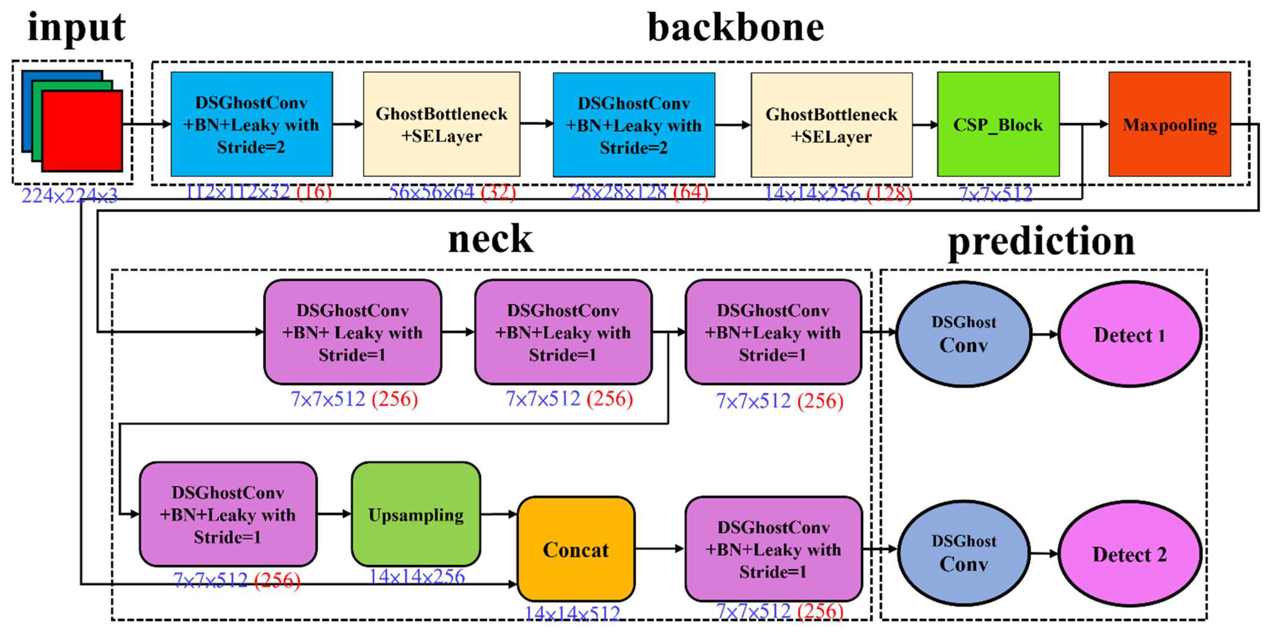
Figure 2.
LWGSE-YOLOv4-tiny architecture [
4]. The number in red indicates the number of filters in convolutions.
Figure 2.
LWGSE-YOLOv4-tiny architecture [
4]. The number in red indicates the number of filters in convolutions.
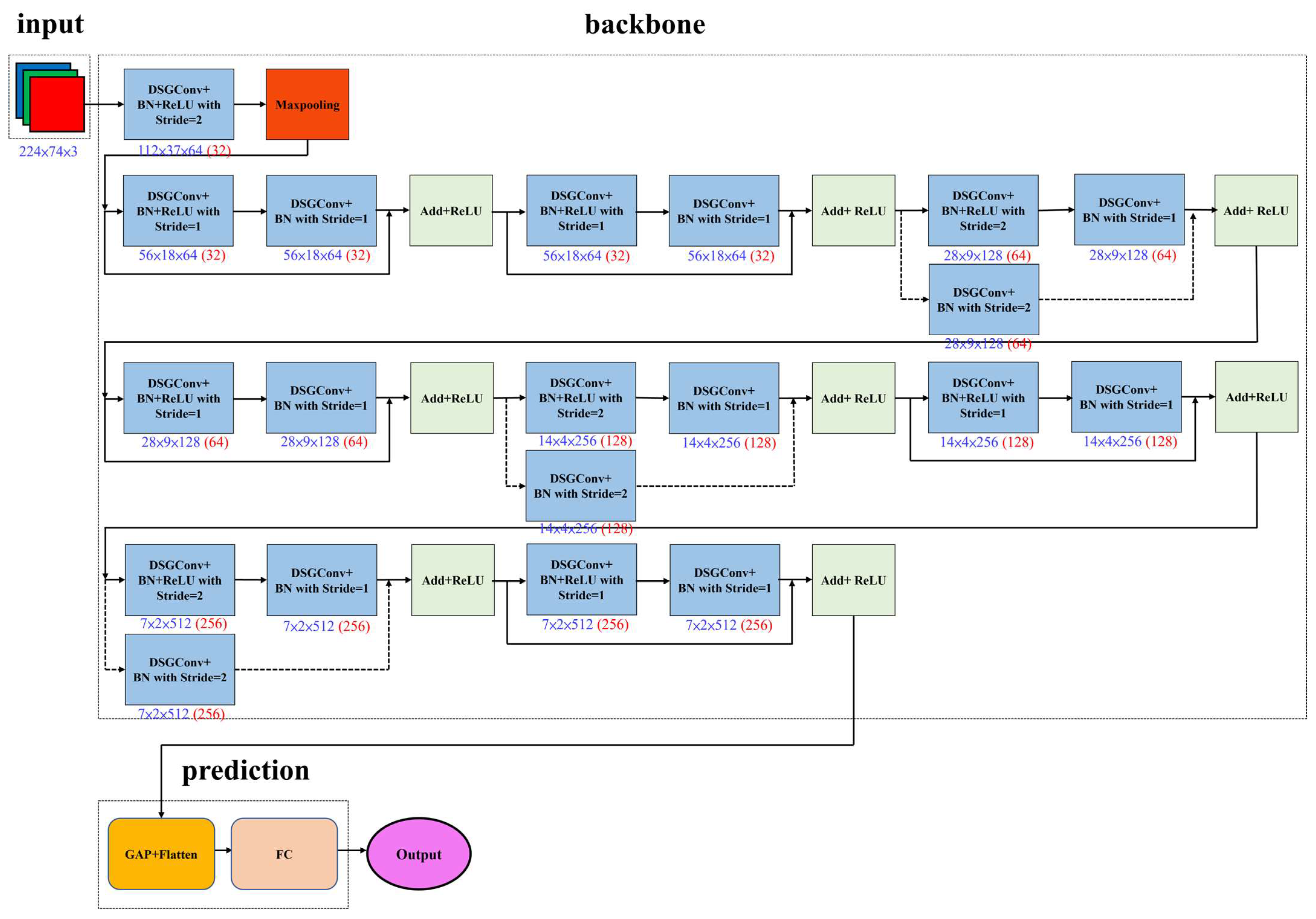
Figure 3.
LWDSG-ResNet18 architecture [
4]. The number in red indicates the number of filters in convolutions.
Figure 3.
LWDSG-ResNet18 architecture [
4]. The number in red indicates the number of filters in convolutions.
Figure 4.
VGG16 architecture.
Figure 4.
VGG16 architecture.
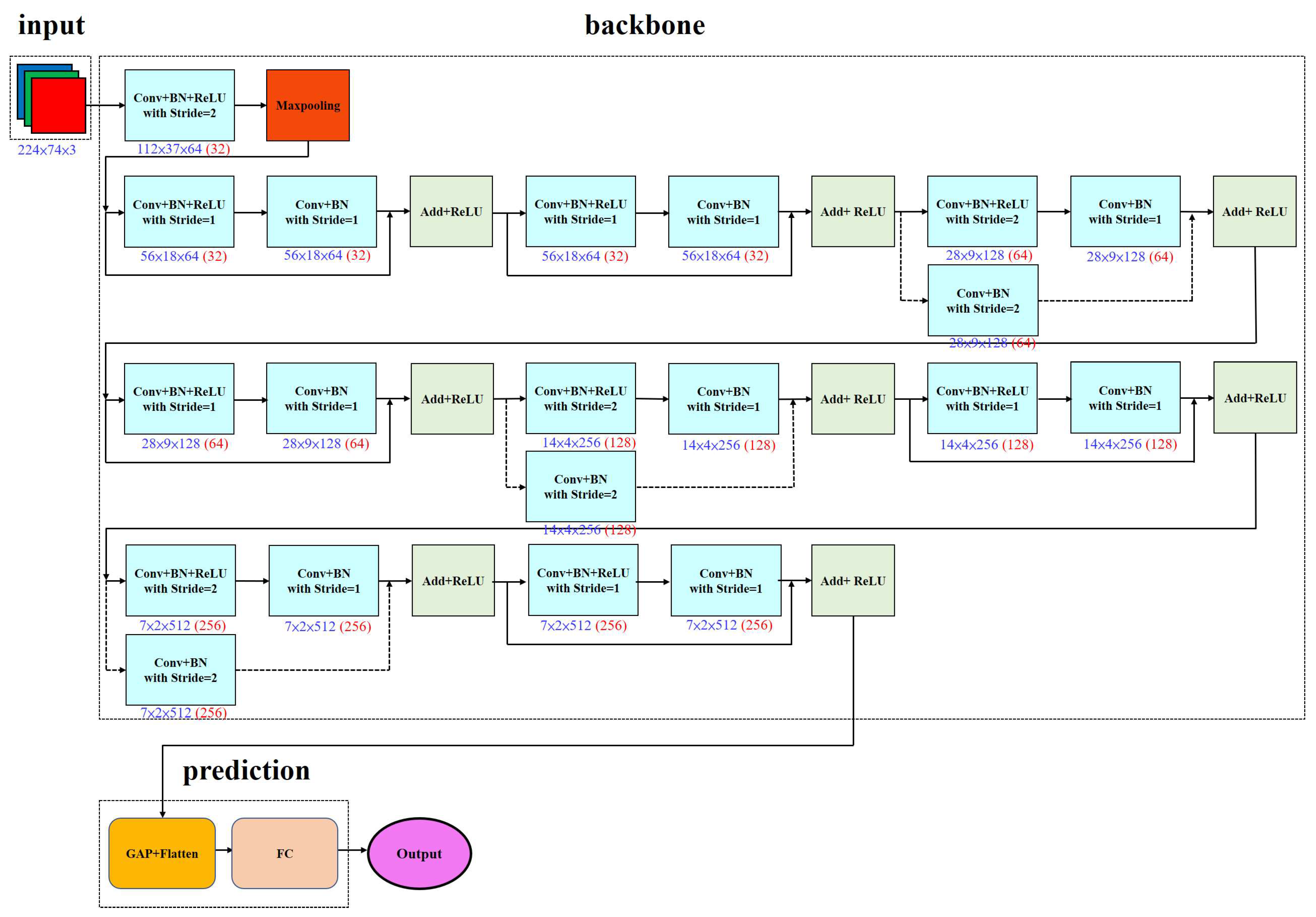
Figure 5.
ResNet18 architecture.
Figure 5.
ResNet18 architecture.
Figure 6.
YOLOv8n architecture.
Figure 6.
YOLOv8n architecture.
Figure 7.
RG-YOLOv8n architecture.
Figure 7.
RG-YOLOv8n architecture.
Figure 8.
YOLOv11n architecture.
Figure 8.
YOLOv11n architecture.
Figure 9.
RG-YOLOv11n architecture.
Figure 9.
RG-YOLOv11n architecture.
Figure 10.
DuCRG-YOLOv11n architecture.
Figure 10.
DuCRG-YOLOv11n architecture.
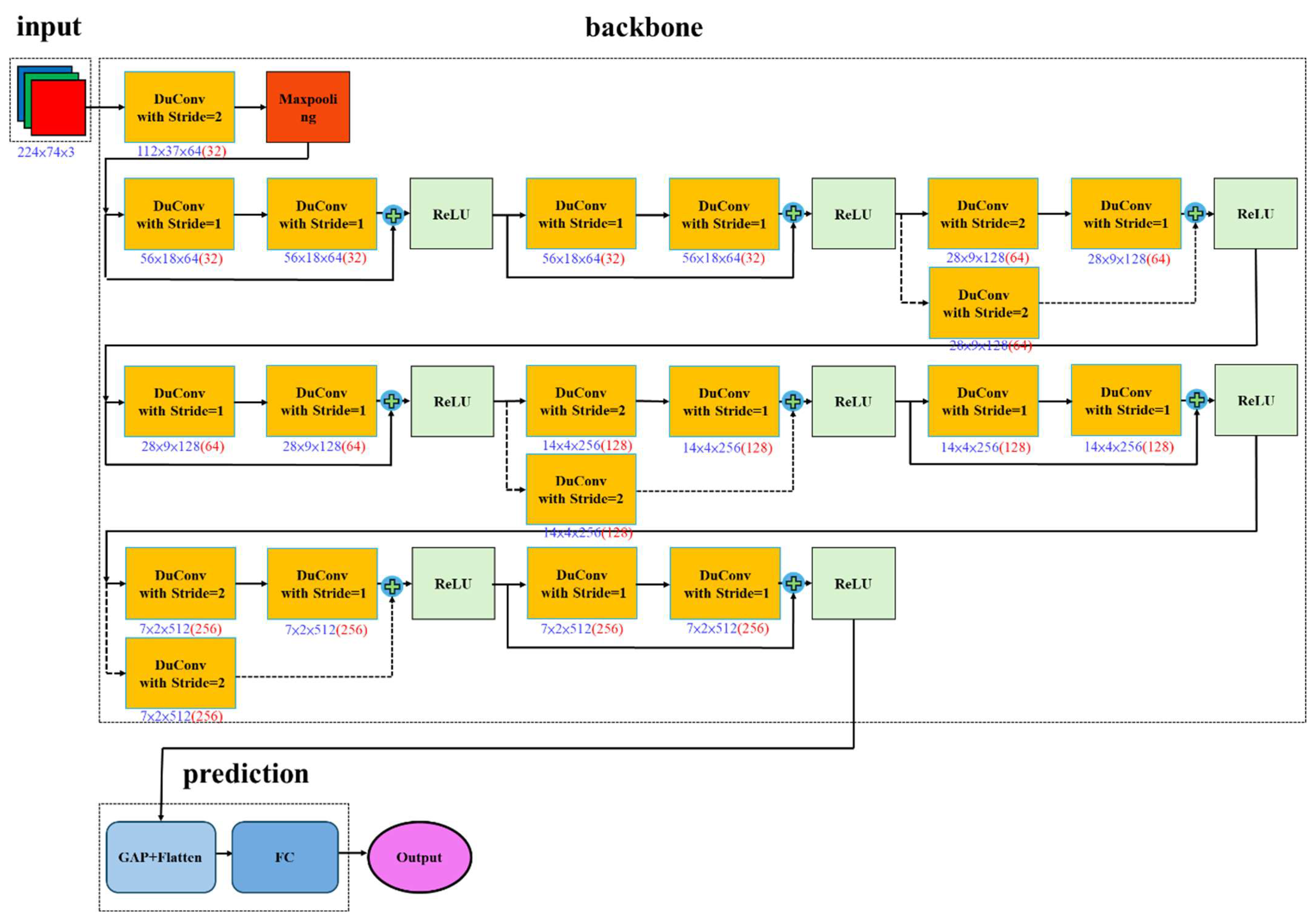
Figure 11.
DuC-ResNet18 architecture. The number in red indicates the number of filters in convolutions.
Figure 11.
DuC-ResNet18 architecture. The number in red indicates the number of filters in convolutions.
Figure 12.
RepGhost bottleneck architecture.
Figure 12.
RepGhost bottleneck architecture.
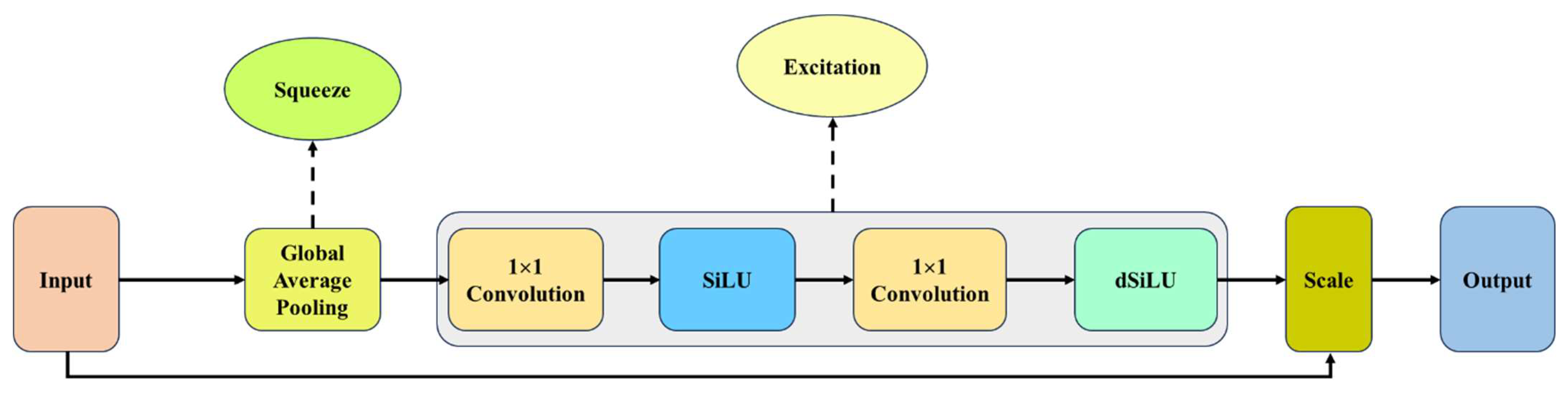
Figure 13.
Derivative of Mobile Squeeze-and-Excitation Layer (dMoSE) architecture.
Figure 13.
Derivative of Mobile Squeeze-and-Excitation Layer (dMoSE) architecture.
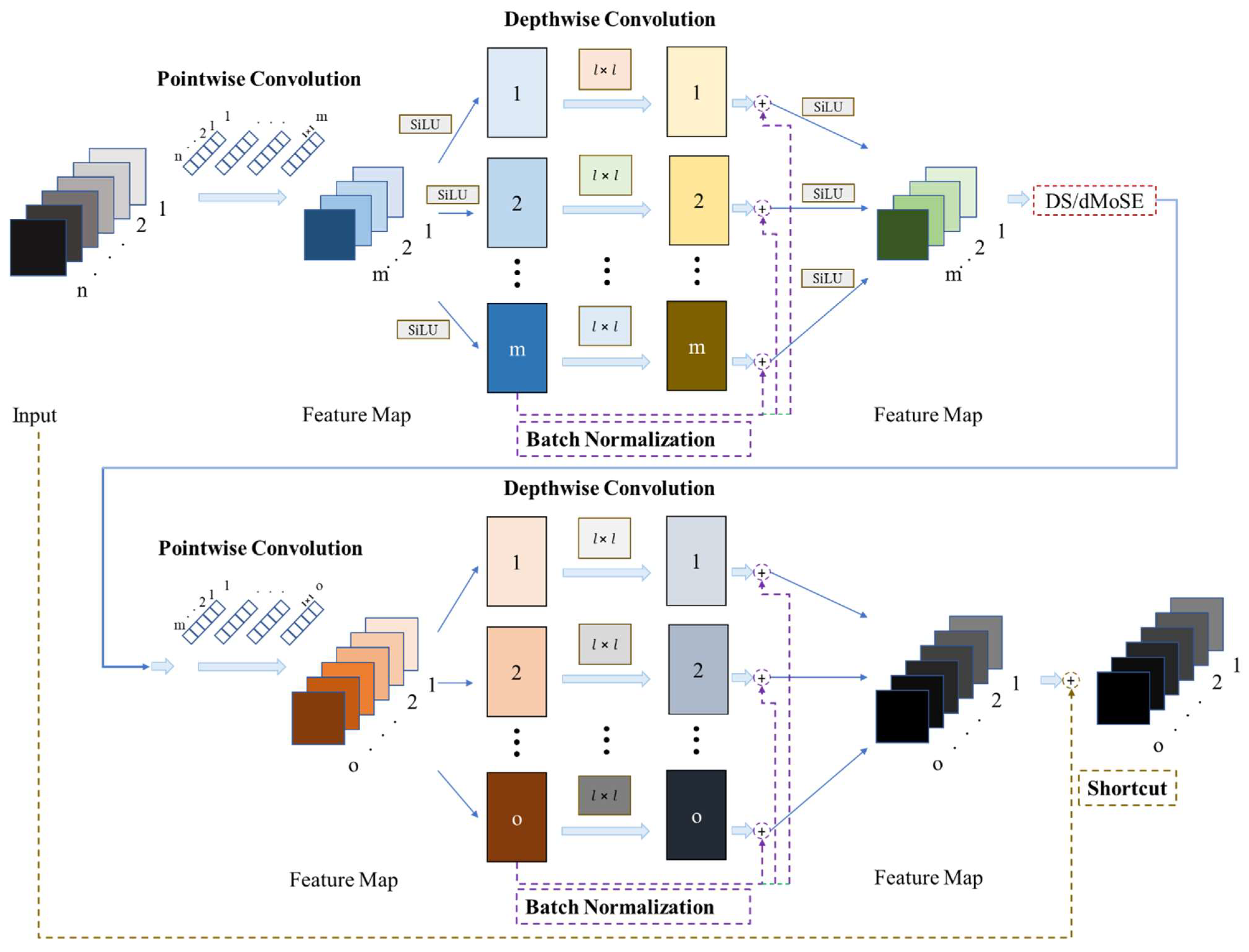
Figure 14.
Dual convolution (DuConv) architecture.
Figure 14.
Dual convolution (DuConv) architecture.
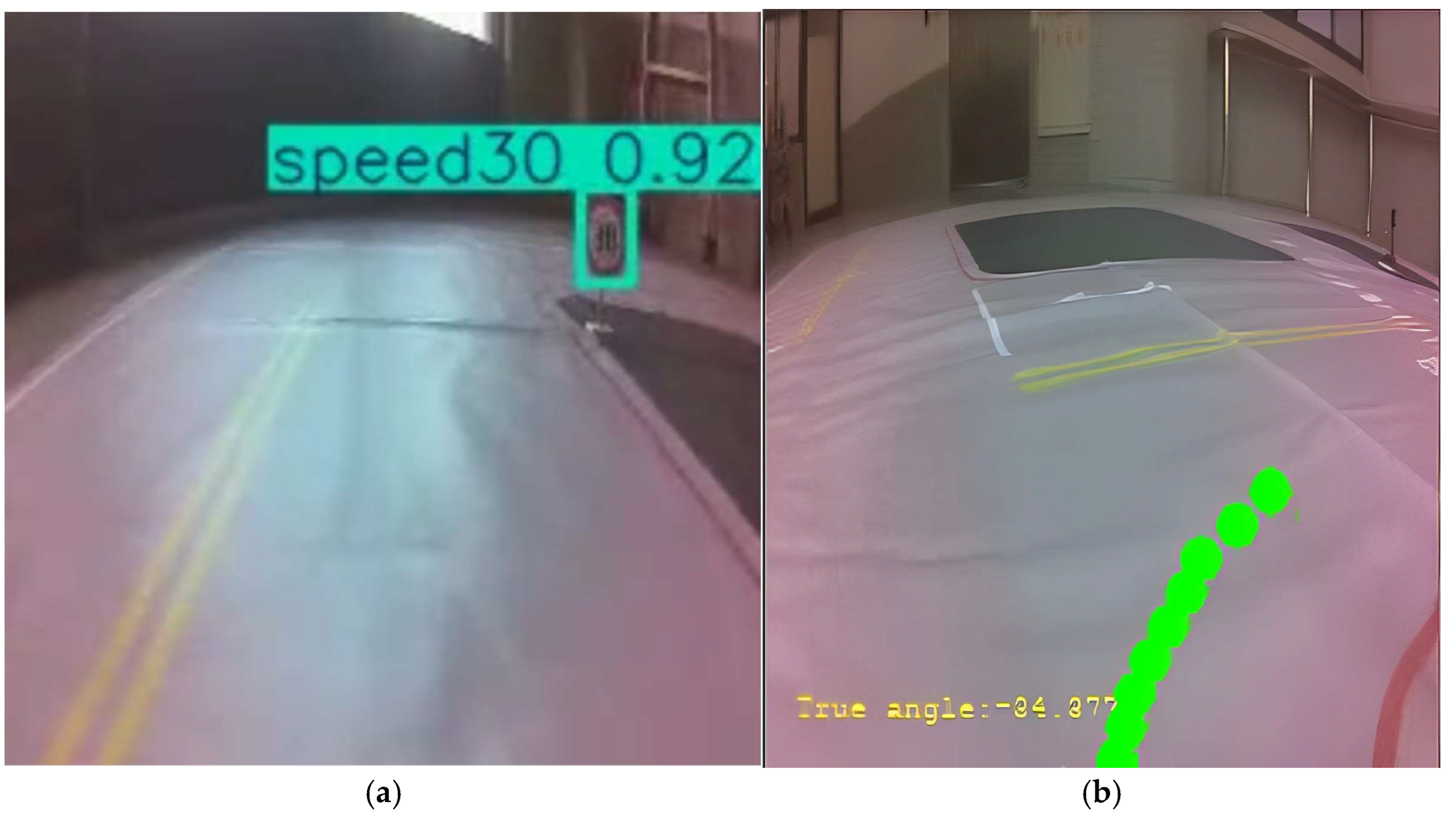
Figure 15.
Live self-driving. (a) DuCRG-YOLOv11n detects objects on the road promptly, and (b) DuC-ResNet18 instantly predicts a steering angle (–34.377) with a green visual indicator on the ground.
Figure 15.
Live self-driving. (a) DuCRG-YOLOv11n detects objects on the road promptly, and (b) DuC-ResNet18 instantly predicts a steering angle (–34.377) with a green visual indicator on the ground.
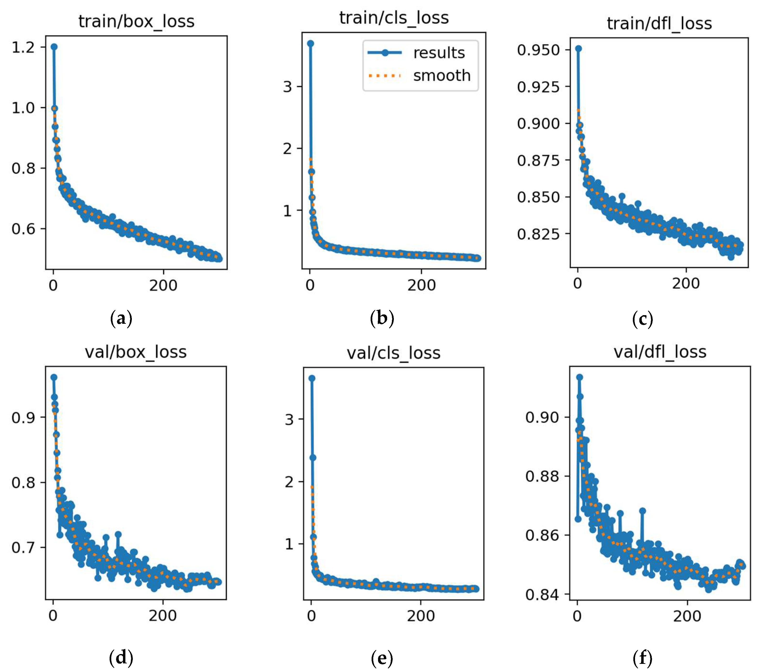
Figure 16.
Training and validation losses for YOLOv8n. (a) Loss in box training. (b) Loss in classification training. (c) Loss in detection training. (d) Loss in box validation. (e) Loss in classification validation. (f) Loss in detection validation. In each plot, the x-axis represents the error value, and the y-axis represents the number of epochs.
Figure 17.
Training and validation losses for RG-YOLOv8n. (a) Loss in box training. (b) Loss in classification training. (c) Loss in detection training. (d) Loss in box validation. (e) Loss in classification validation. (f) Loss in detection validation. In each plot, the x-axis represents the error value, and the y-axis represents the number of epochs.
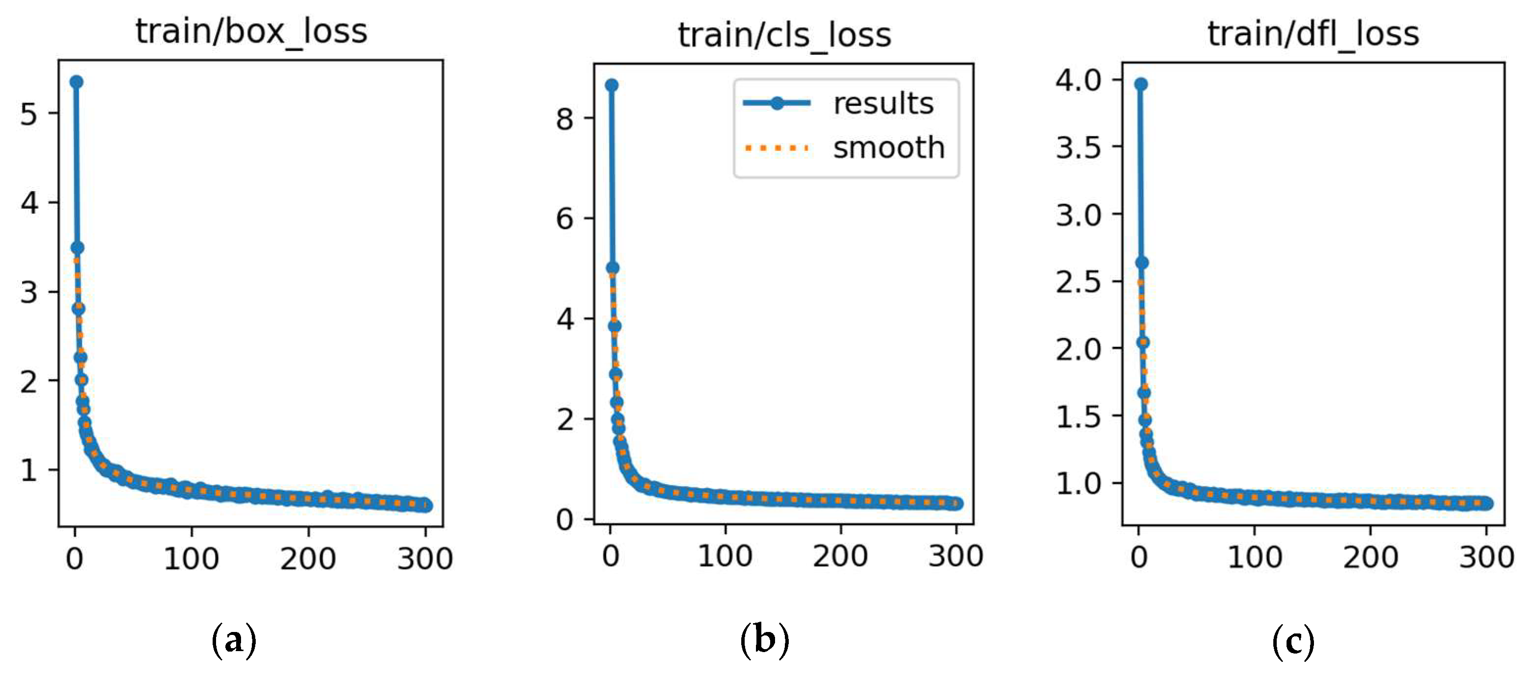
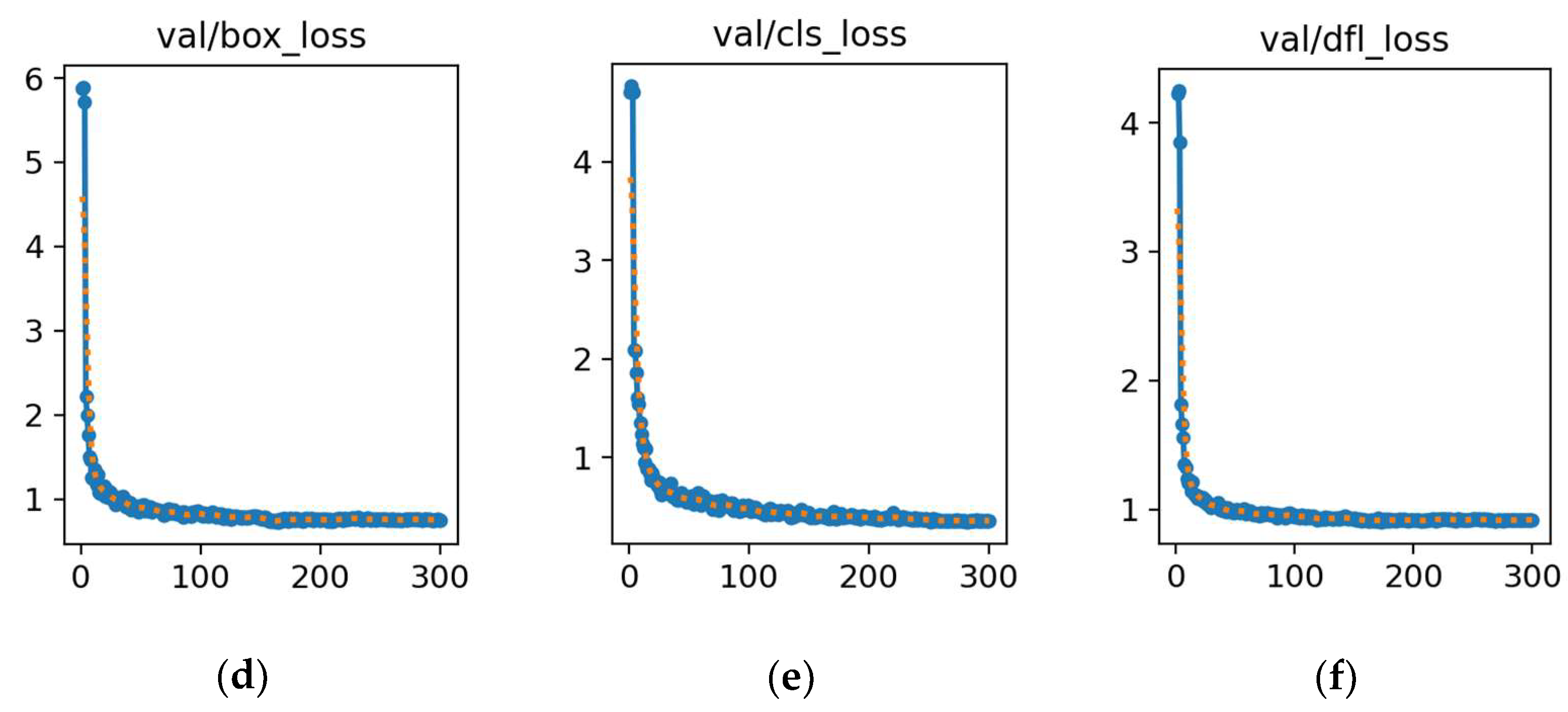
Figure 18.
Training and validation losses for YOLOv11n. (a) Loss in box training. (b) Loss in classification training. (c) Loss in detection training. (d) Loss in box validation. (e) Loss in classification validation. (f) Loss in detection validation. In each plot, the x-axis represents the error value, and the y-axis represents the number of epochs.
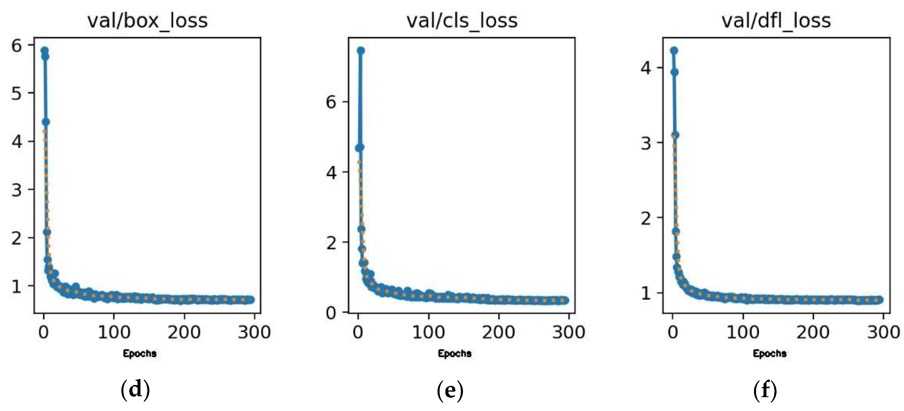
Figure 19.
Training and validation losses for RG-YOLOv11n. (a) Loss in box training. (b) Loss in classification training. (c) Loss in detection training. (d) Loss in box validation. (e) Loss in classification validation. (f) Loss in detection validation. In each plot, the x-axis represents the error value, and the y-axis represents the number of epochs.
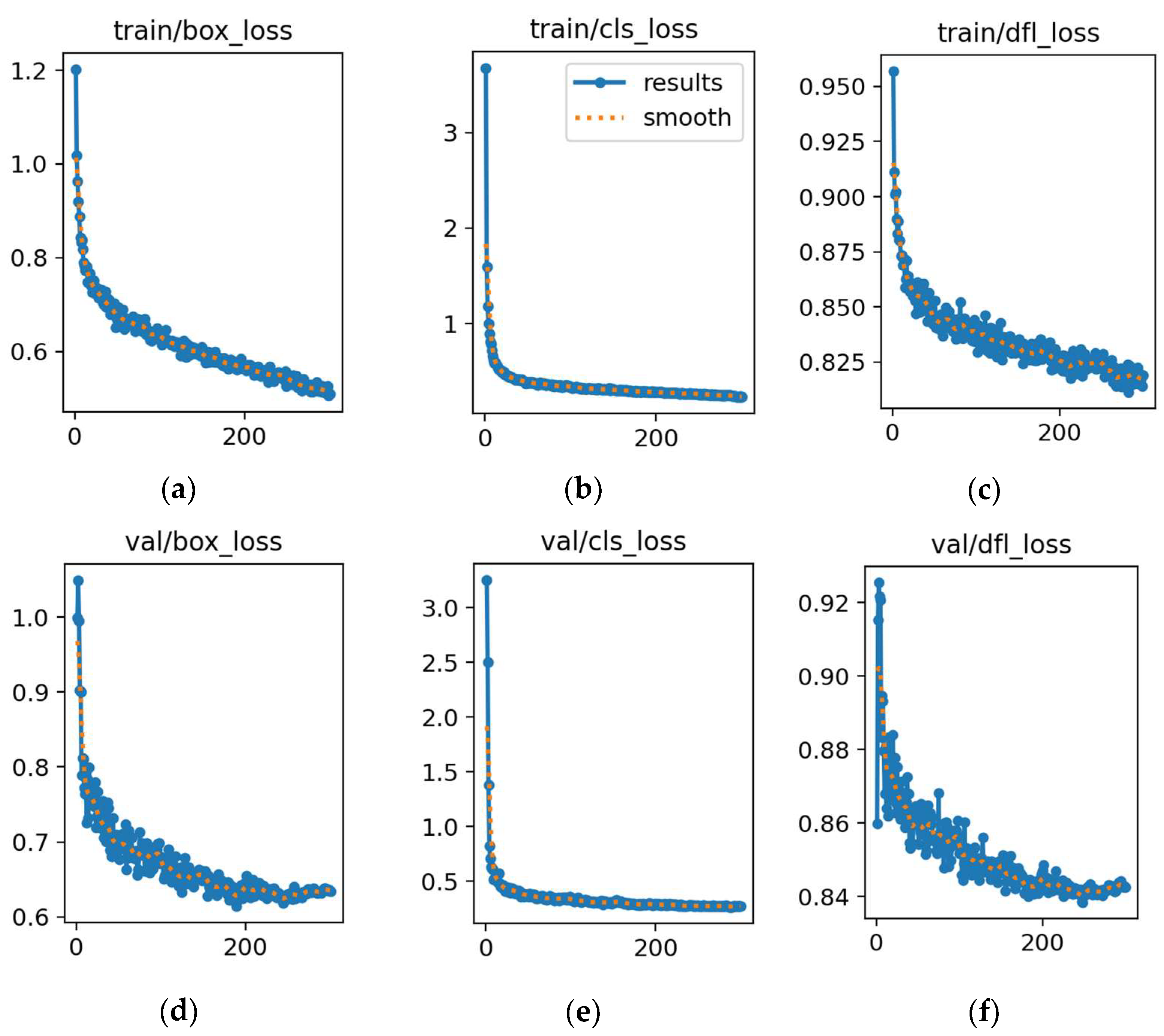
Figure 20.
Training and validation losses for DuCRG-YOLOv11n. (a) Loss in box training. (b) Loss in classification training. (c) Loss in detection training. (d) Loss in box validation. (e) Loss in classification validation. (f) Loss in detection validation. In each plot, the x-axis represents the error value, and the y-axis represents the number of epochs.
Figure 21.
Losses in training and validation for DuC-ResNet18.
Figure 21.
Losses in training and validation for DuC-ResNet18.
Figure 22.
Precision–recall curve for DuCRG-YOLOv11n.
Figure 22.
Precision–recall curve for DuCRG-YOLOv11n.
Figure 23.
The MSE of predicted and actual steering angle using Du-ResNet18.
Figure 23.
The MSE of predicted and actual steering angle using Du-ResNet18.
Table 1.
Hardware specification.
Table 1.
Hardware specification.
| Unit | Component |
|---|
| CPU | Intel(R) Core(TM) i7-13700H CPU @ 3.60 GHz |
| GPU | NVIDIA GeForce GTX 4070 Ti |
| Memory | DDR5-5600 RAM 16 GB × 4 |
| Storage | CT1000MX500SSD1 1TB |
Table 2.
Recipe of packages.
Table 2.
Recipe of packages.
| Software | Version |
|---|
| Python | 3.8.12 |
| Pytorch | 1.9.1 |
| Anaconda | 23.7.2 |
| JetPack | 4.6 |
| Jupyter | 1.0.0 |
Table 3.
Components of NVIDIA Jetson Nano.
Table 3.
Components of NVIDIA Jetson Nano.
| Unit | Component |
|---|
| CPU | Quad-core ARM Cortex-A57 MPCore Processor |
| GPU | NVIDIA Maxwell Architecture with 128 NVIDIA CUDA® cores |
| Memory | 4 GB 64-bit LPDDR4, 1600 MHz 25.6 GB/s |
| Storage | 16 GB eMMC 5.1 |
Table 4.
Time required to train and infer detecting objects for models.
Table 4.
Time required to train and infer detecting objects for models.
| Metrics | YOLOv8n | RG-YOLOv8n | YOLOv11n | RG-YOLOv11n | DuCRG-YOLOv11n |
|---|
| Training (h) | 1 | 2.3 | 2.0 | 2.8 | 3.0 |
| Inference (ms) | 0.8 | 0.9 | 0.9 | 1.1 | 0.7 |
Table 5.
Time to train and infer predicting steering angles for models.
Table 5.
Time to train and infer predicting steering angles for models.
| Metrics | VGG16 | ResNet18 | RG-ResNet18 | DuC-ResNet18 |
|---|
| Training (s) | 1480 | 2480 | 3245 | 2853 |
| Inference (ms) | 21.27 | 25.18 | 27.40 | 17.50 |
Table 6.
Parameters of detecting object models.
Table 6.
Parameters of detecting object models.
| Metrics | YOLOv8n | RG-YOLOv8n | YOLOv11n | RG-YOLOv11n | DuCRG-YOLOv11n |
|---|
| # of parameters | 3,007,403 | 2,300,987 | 2,605,187 | 2,529,259 | 1,412,752 |
Table 7.
Parameters of predicting steering angle models.
Table 7.
Parameters of predicting steering angle models.
| Metrics | VGG16 | ResNet18 | RG-ResNet18 | DuC-ResNet18 |
|---|
| # of parameters | 14,719,938 | 11,177,538 | 11,103,490 | 1,447,234 |
Table 8.
Speed and precision of detecting objects.
Table 8.
Speed and precision of detecting objects.
| Metrics | YOLOv8n | RG-YOLOv8n | YOLOv11n | RG-YOLOv11n | DuCRG-YOLOv11n |
|---|
| FPS | 125 | 129 | 128 | 131 | 147 |
| Precision (%) | 97.1 | 97.5 | 99.0 | 99.2 | 99.1 |
Table 9.
Speed and loss of predicting steering angles.
Table 9.
Speed and loss of predicting steering angles.
| Metrics | VGG16 | ResNet18 | RG-ResNet18 | DuC-ResNet18 |
|---|
| FPS | 31.9 | 27.0 | 48.34 | 57.13 |
| MSE | 0.0849 | 0.0712 | 0.0019 | 0.0587 |
Table 10.
FPS of model combination.
Table 10.
FPS of model combination.
| O. D. | YOLOv8n | RG-YOLOv8n | YOLOv11n | RG-YOLOv11n | DuCRG-YOLOv11n |
|---|
| St. A. P. | |
|---|
| VGG16 | 25.4 | 25.6 | 25.5 | 25.7 | 25.9 |
| ResNet18 | 37.1 | 37.4 | 37.3 | 37.6 | 37.8 |
| RG-ResNet18 | 38.6 | 42.1 | 40.0 | 43.8 | 44.5 |
| DuC-ResNet18 | 43.1 | 48.6 | 44.7 | 49.6 | 50.7 |
| Average | 36.0 | 38.4 | 36.8 | 39.0 | 39.72 |
Table 11.
Accuracy and precision of model combination.
Table 11.
Accuracy and precision of model combination.
| Precision(%) | O. D. |
|---|
| MSE | | YOLOv8n | RG-YOLOv8n | YOLOv11n | RG-YOLOv11n | DuCRG-YOLOv11n |
|---|
| St. A. P. | VGG16 | (0.0849, 97.1) | (0.0849, 97.5) | (0.0849, 99.0) | (0.0849, 99.2) | (0.0849, 99.1) |
| Resnet18 | (0.0712, 97.1) | (0.0712, 97.5) | (0.0712, 99.0) | (0.0712, 99.2) | (0.0712, 99.1) |
| RG-ResNet18 | (0.0019, 97.1) | (0.0019, 97.5) | (0.0019, 99.0) | (0.0019, 99.2) | (0.0019, 99.1) |
| DuC-ResNet18 | (0.0578, 97.1) | (0.0578, 97.5) | (0.0578, 99.0) | (0.0578, 99.2) | (0.0578, 99.1) |


