Implementing High-Speed Object Detection and Steering Angle Prediction for Self-Driving Control

Abstract

In the previous work, we proposed LWGSE-YOLOv4-tiny and LWDSG-ResNet18, leveraging depthwise separable and Ghost Convolutions for fast self-driving control while achieving a detection speed of 24.9 FPS. However, the system fell short of Level 4 autonomous driving safety requirements. That is, the control response speed of object detection integrated with steering angle prediction must exceed 39.2 FPS. This study enhances YOLOv11n with dual convolution and RepGhost bottleneck, forming DuCRG-YOLOv11n, significantly improving the object detection speed while maintaining accuracy. Similarly, DuC-ResNet18 improves steering angle prediction speed and accuracy. Our approach achieves 50.7 FPS, meeting Level 4 safety standards. Compared to previous work, DuCRG-YOLOv11n boosts feature extraction speed by 912.97%, while DuC-ResNet18 enhances prediction speed by 45.37% and accuracy by 12.26%.

1. Introduction

Automakers and tech companies are working together to advance fully autonomous driving technology. Current Level 1 and Level 2 self-driving cars can carry out Advanced Driver Assistance Systems (ADAS), which include onboard cameras, Camera-Monitor Systems (CMS), and Head-Up Displays (HUDs) to enhance situational awareness and driving safety. Further improvements, like long-wave infrared cameras, help CMS operate in low-light conditions, reducing glare and improving night-time driving safety. AR HUDs project driving information within the driver’s field of vision, assisting without distractions.

In Q4 2023, Mercedes-Benz Drive Pilot became one of the few Level 3 self-driving cars compliant with EU UN R157 regulations, receiving sales approval in Germany, Nevada, and California. In 2024, BMW cars with personal pilot were also approved in Germany, outperforming the personal pilot of Mercedes cars by functioning in the dark. Meanwhile, Tesla unveiled its Level 4 autonomous taxi, called Cybercab, and other high-tech vehicles in October 2024. Tech giants like Qualcomm and NVIDIA are racing to develop high-performance automotive chips to support the increased computational demands of Level 4 autonomous driving. Therefore, self-driving cars require ultra-fast object detection and image recognition to achieve L4 safety.

Real-time fusion of detecting objects and predicting steering angles is essential for precise control responses. YOLOv4-tiny [1] enables the fast detection of vehicles and traffic signs, while ResNet18 [2] accurately predicts steering angles at intersections or multi-lane roads. Our previous work [3] introduced lightweight models, LW-YOLOv4-tiny and LW-ResNet18, which improved object detection and steering angle prediction for faster autonomous driving responses. However, speed limitations still caused delayed steering predictions, increasing the number of dangerous car accidents. Further acceleration of LW-YOLOv4-tiny and LW-ResNet18 is necessary because the speed is much higher than the accuracy.

Previous work [4] incorporated GhostBottleneck [5] and SELayer [6] to replace CSP_Block, resulting in the lightweight LWGSE-YOLOv4-tiny model. Meanwhile, LWDSG-ResNet18 used depthwise separable convolution [7] to enhance computing speed and pattern recognition accuracy. Despite these improvements to achieve the detecting speed of 24.9 FPS, the system failed to meet L4 safety standards, requiring a control response speed exceeding 39.2 FPS. To achieve this, we sought a high-speed visual detection method capable of both rapid response and high accuracy.

This study introduces a new high-speed autonomous driving method to replace LWGSE-YOLOv4-tiny and LWDSG-ResNet18. By integrating RepGhost bottleneck [8] with SELayer [6] in YOLOv11n, we replace the C3k2 bottleneck and introduce Dual Conv [9] (Depthwise Separable Conv + Point Conv) to replace standard Conv layers (resulting in DuCRG-YOLOv11n). These modifications enable faster inference while maintaining high detection accuracy. RepGhost bottleneck ensures consistent feature map dimensions, allowing for more prosperous feature extraction. For ResNet18, we replace standard Conv layers with Dual Conv, forming DuC-ResNet18, achieving high-speed and high-accuracy predictions. Our approach significantly accelerates inference time, reducing autonomous driving control latency and meeting L4 safety requirements [10]. Specifically, our method achieves a control response speed of 50.7 FPS, a key contribution of this study. Following previous work [4], a model car, NVIDIA JetRacer [11], was used to simulate autonomous driving in urban environments. This study also evaluates various YOLO-related models concerning object detection and ResNet-related models focusing on steering angle prediction to identify the most efficient solution for real-time self-driving control.

2. Related Work

2.1. Literature Review

This section summarizes research on advanced visual algorithms for fast object detection. Dong et al. [12] proposed C3Ghost and Ghost blocks in YOLOv5 to reduce floating-point operations (FLOPs) in feature fusion, enhancing feature representation. To improve accuracy, they integrated a convolutional block attention module (CBAM) in the backbone to emphasize critical vehicle detection features while suppressing irrelevant ones. Additionally, they applied CIoU_Loss for faster and more accurate bounding box regression. Their model increased detection accuracy by 3.2%, reduced FLOPs by 15.24%, and decreased parameters by 19.37% compared to standard YOLOv5.Carrasco et al. [13] enhanced YOLOv5 with multi-scale modules and spatial/channel attention, improving accuracy from 63.87% to 96.34% for a specific application. They also developed a single-branch YOLOv5 solution that achieved higher speeds than YOLOv5 while maintaining precision comparable to a multi-branch solution. Momin et al. [14] adapted YOLOv4-tiny for aerial vehicles, adding an extra-scale feature map, resulting in three prediction heads. Expanding the second and third feature map sizes can considerably improve small vehicle detection in aerial images, achieving performance comparable to newer YOLO versions. Cai et al. [15] designed a YOLOv8-RepGhost-EMA algorithm for embedded systems, integrating EMA attention and RepGhost modules for lightweight optimization. Applied to waste detection, their model reduced parameters by 13% and improved precision by 4%, recall by 1.1%, and mean average precision (mAP) by 1.9%. Their work contributed valuable insights for lightweight underwater object detection, balancing accuracy and speed. Wang et al. [16] modified YOLOv8 by structurally reparameterizing its backbone using Diverse Branch Block (DBB). They incorporated multiple scale features and a bidirectional feature pyramid network (BiFPN) to enhance small object detection. Their model achieved 64.5% accuracy on the SODA-A dataset while reducing the computational cost to 7.1 GFLOPs, making it ideal for commercial highway driving applications. Chang et al. [5] combined Ghost Conv and depthwise convolution (DW Conv) into YOLOv4-tiny for rapidly detecting objects (LWGSE-YOLOv4-tiny) and ResNet18 for quickly predicting steering angles (LWDSG-ResNet18). Their approach achieved a speed of 56.1 FPS. It resulted in a mean-squared-error (MSE) of 0.0683, validated on a Jetson Nano and NVIDIA GTX 1080Ti with 128 NVIDIA CUDA cores under the Maxwell architecture.

2.2. Requirements for L4-Level Safe Self-Driving

L4 autonomous driving refers to highly automated driving where the vehicle can operate independently, even without passengers. It must reach a safe state without human intervention, such as stopping in a parking lot [17]. However, its autonomy is still subject to certain conditions, such as following predefined routes, operating on highways, or maneuvering in parking lots. To meet the safety requirements of L4 autonomous driving [17], a vehicle driving on highway roads needs to maintain a safe following distance, which consists of the reaction distance ($S_r$) and braking distance ($S_b$). At a speed of 100 km/h, the highway authority recommends a minimum safe following distance of 50 m [18], denoted as $S_f$. Considering the required L4 autonomous driving safety distance, the sum of reaction and braking distance must be within 50 m. Equation (1) calculates the emergency braking distance, where $S_b$ is the braking distance (m), $v$ is the vehicle speed (m/s), $g$ represents gravitational acceleration (9.8 m/s²), and $\mu$ is the friction coefficient (typically 0.7–0.8 for tires on dry roads). Self-driving cars must be capable of high-speed object detection and image recognition within a very short reaction distance to meet the requirement of L4 safety driving on highway roads. This requirement is crucial for making timely decisions in emergency braking situations. Equation (2) estimates the required object detection frequency, where ${\mathrm{f}}_d$ is the frames per second (FPS) of detecting objects and recognizing images, $S_f$ represents the following distance (m), and $S_b$ stands for the braking distance (m).

$$S_b={\displaystyle v^2/2g\mu }$$

(1)

$${\mathrm{f}}_d={\displaystyle 1/\left(\frac{S_r}{v}\right)}, where S_r=S_f-S_b$$

(2)

First, we convert a 100 km/h speed to 27.8 m/s, then substitute it into Equation (1) to calculate the emergency braking distance, which comes out to 49.29 m. Next, by subtracting the braking distance from the following distance (50 m–49.29 m), we obtain a reaction distance of 0.71 m. Then, using Equation (2), we estimate the required object detection frequency for high-speed response, which is 39.2 FPS. As a result, the frames per second (FPS) of detecting objects and recognizing images of 39.2 FPS meet the requirements for L4 safe self-driving on highways.

2.3. Configuration of Simulation Environment

In the previous work [5], the NVIDIA JetRacer demonstrated a small model car that implemented self-driving scenarios. The NVIDIA Jetson Nano powers the JetRacer and can behave as an autonomous AI race car. Users can access it via a web browser for simulation examples and interactive programming. The optimized JetRacer can reach high-speed motion with high frame rates. Seven cameras were strategically positioned around the JetRacer to construct an autonomous driving scenario, enabling it to navigate and conduct simulation-based autonomous driving tests on a planar road map, as shown in Figure 1. Figure 1 demonstrates that the planar road map installed minor traffic lights, turn signs, speed limit signs, etc., and users can operate the JetRacer to drive while following traffic rules. The currently simulated scenario using the lightweight model from our previous work [4] still cannot meet the requirements of L4 safe autonomous driving; that is, the control response speed of object detection integrated with steering angle prediction must exceed 39.2FPS. This study aims to achieve the requirements of L4 safe autonomous driving.

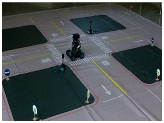
Figure 1. Planar road map and model car [5].

2.4. Fast-Response LWGSE-YOLOv4-Tiny and LWDSG-ResNet18 Models

In previous work [4], Figure 2 shows that the lightweight network LWGSE-YOLOv4-tiny, which detects objects fast, has an improved response time. Figure 3 shows that LWDSG-ResNet18, which predicts steering angles quickly, also has enhanced driving control. The proposed two lightweight models consume less power when executing self-driving control. Our other study [4] described a detailed execution flow for information fusion and visual-assisted steering. Compared with [3], the two approaches proposed in [4] can better detect objects and predict steering angles.

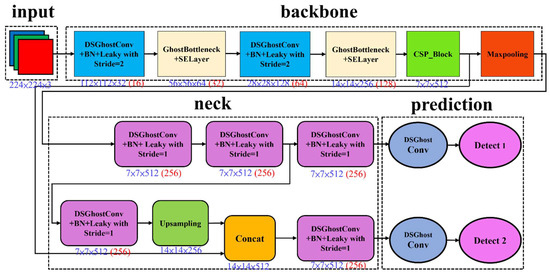
Figure 2. LWGSE-YOLOv4-tiny architecture [4]. The number in red indicates the number of filters in convolutions.

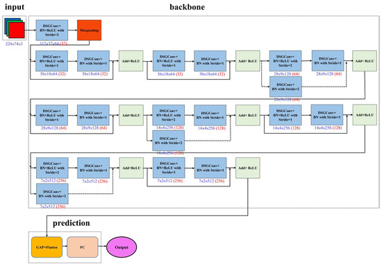
Figure 3. LWDSG-ResNet18 architecture [4]. The number in red indicates the number of filters in convolutions.

2.5. VGG16 Model

In Figure 4, VGG16 [19] is a classic CNN model proposed by the Visual Geometry Group (VGG) at the University of Oxford in 2014 for image classification tasks. Its key feature is stacking multiple 3 × 3 convolutional layers to enhance feature extraction capabilities. This model used ReLU as the activation function between each convolution, and max-pooling layers were employed to shrink the size of the feature maps. Among the VGG models, VGG16 and VGG19 are particularly notable, with VGG16 using fewer layers than VGG19. Applications widely adopted this simple yet effective architecture, integrating it as the backbone for feature extraction in later object detection models, utilizing either VGG16 or VGG19.

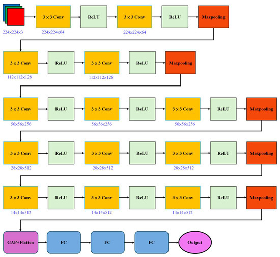
Figure 4. VGG16 architecture.

2.6. ResNet18 Model

ResNet refers to the Residual Network [2], proposed by Microsoft Research in 2015. This model designed ResNet to address the “degradation problem” in deep networks (where deeper networks perform worse). The core technology is its residual block, where the model adds the output after convolution to the input. This design allows for smooth backpropagation of gradients and prevents gradient vanishing issues as the network depth increases, making it easier to build deeper networks. Among the ResNet series, ResNet18 is the most lightweight version, with 18 layers, making it suitable for resource-limited situations. Figure 5 shows its specific architecture.

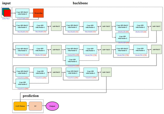
Figure 5. ResNet18 architecture.

2.7. YOLOv8n Model

YOLOv8 [20] improves YOLOv5, incorporating a more efficient anchor-free design. In Figure 6, the backbone of YOLOv8 utilizes the C2f block to extract hierarchical features effectively, whereas an enhanced version of the C3 block is used in the C2f block. Based on the C3 block, the C2f block draws inspiration from the ELAN block in YOLOv7 [21]. It allows C2f to achieve richer functionality while maintaining a lightweight structure. The feature pyramid network (FPN) [22] has also been simplified and embedded into the neck to strengthen multiple-scale feature representation. In YOLOv8, the head segregates objectness, classification, and regression tasks, improving accuracy without incurring a severe computational load. This part intends to streamline the detection process and coordinate the network’s adaptability to various object sizes and aspect ratios [23]. The system architecture balances speed and accuracy, making YOLOv8 well-suited for real-time applications. In Figure 7, this study also replaced the bottleneck in YOLOv8n with the RepGhost bottleneck(RG-YOLOv8n) as an experimental control.

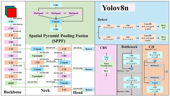
Figure 6. YOLOv8n architecture.

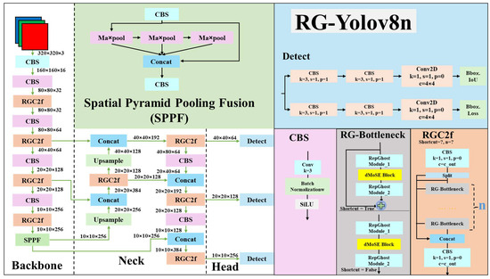
Figure 7. RG-YOLOv8n architecture.

2.8. YOLOv11n Model

YOLOv11 [20] makes further improvements to the YOLOv8 architecture, as shown in Figure 7. In Figure 7, YOLOv11 introduces the C3k2 module to replace the C2f module in the YOLOv8 architecture. With an additional parameter, C3k, the C3k2 module inherits the properties of C2f. When the condition sets C3k to False, C3k2 behaves the same as C2f. When the condition sets C3k to True, the C3k2 module replaces the bottleneck in C2f with half of the output channels of C3k. This modification considerably boosts inference efficiency and increases the power of extracting features. Mainly, YOLOv11 adopts the C2PSA module, embedding the polarized self-attention (PSA) [24] into the previous version C2 of C2f. This feature combines polarization filtering, high-quality pixel-level regression, and enhanced design with two key features. In Figure 8, YOLOv11 changes the detection module (Detect) by adding two more depthwise separable convolutions (DW Conv) in the Bbox Loss [25]. This mechanism can decrease the number of parameters and reduce computational costs in computing convolution while improving representation efficiency. In Figure 9, this study also replaced the bottleneck in YOLOv11n with the RepGhost bottleneck (RG-YOLOv11n) as an experimental control.

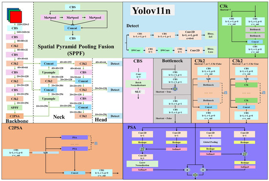
Figure 8. YOLOv11n architecture.

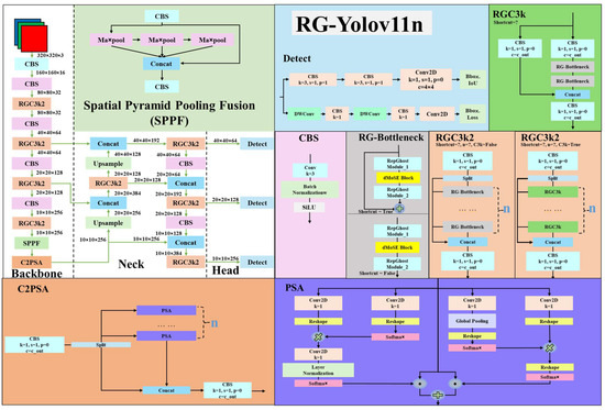
Figure 9. RG-YOLOv11n architecture.

3. Methods

3.1. High-Speed Response Using DuCRG-YOLOv11n and DuC-ResNet18 Models

Although YOLOv11n and ResNet18 are already relatively fast models, when implemented in real-world self-driving for environmental object detection and image recognition, the vehicle control response time still needs to be reduced. Therefore, there is a need to improve the inference performance of the model. We aim to lower the computational load, reduce the response time while the self-driving control is active, and reduce erroneous critical decisions in control. The improved model can also decrease power consumption by reducing the number of convolutions to make it energy-efficient. Based on the RepGhost [8] and DualConv [9] studies, this study proposes an improved architecture for YOLOv11n to build a robust model detecting objects, denoted DuCRG-YOLOv11n, as shown in Figure 10. Furthermore, this study applied the DualConv method to construct a reformed model predicting steering angles, denoted DuC-ResNet18, as shown in Figure 11.

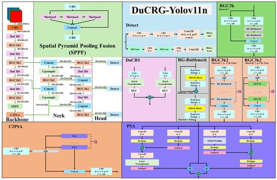
Figure 10. DuCRG-YOLOv11n architecture.

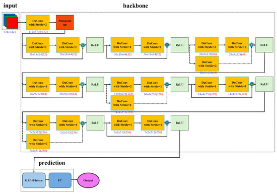
Figure 11. DuC-ResNet18 architecture. The number in red indicates the number of filters in convolutions.

The proposed DuCRG-YOLOv11n replaces the bottleneck module in the C3k2 block of YOLOv11n with the RepGhost bottleneck module [8], as shown in Figure 10. The improvement in the RepGhost block lies in using the addition operation to replace the concatenation operation in Ghost Conv [5]. This change reduces memory usage during computation, and since the addition operation does not alter the shape of the feature maps, it helps lighten the computational burden, leading to faster results. The RepGhost block retains the linear transformation from Ghost, preserving the key characteristics of Ghost features. As a result, even though the algorithm simplifies traditional convolutions, it retains more features, enhancing the model’s computation speed.

Additionally, the RepGhost block incorporates the reparameterization technique from Rep, which adds the trained batch normalization (BN) weights to the Ghost Conv weights. This integrated weight allows the deep model to maintain the same precision as traditional convolutions while being faster and more lightweight during inference, thereby improving computation speed. Algorithm 1 provides a detailed statement of the execution flow of the RepGhost block. The proposed DuC-ResNet18 and DuCRG-YOLOv11n also use the DuConv module [9] to replace the conventional Conv module, as shown in Figure 10 and Figure 11. By combining depthwise convolution (DW Conv) with pointwise convolution (PW Conv), this module significantly reduces the computational load of traditional convolutions. Moreover, combining these two convolution types enables feature extraction at two scales, helping maintain the model’s accuracy.

Algorithm 1 RepGhost Block (RG Block) [8]

$\mathrm{Input}: \mathrm{Image} X$$, \mathrm{ghost} \mathrm{modules} \mathrm{with} \mathrm{linear} \mathrm{transformation} \mathrm{functions} {\mathsf{\phi }}_i$ $\mathrm{Output}: Outfm$ Compute the output of the pointwise convolution: ${Insfm}_i={\mu }_{h,i}\left({fm}_h\right)={fm}_h\odot {pf}_{i,P}$ $\forall h=\mathrm{1,2},\dots ,N, i=\mathrm{1,2},\dots ,M, P=\{\mathrm{1,2},\dots ,N\}$ $\mathrm{where} {\mathsf{\mu }}_{h,i}$ represents a pointwise convolution to obtain intrinsic feature maps ${Insfm}_i$$, \odot$ stands for a point-to-point product of the sum between the feature map ${fm}_h$ and pointwise filter ${pf}_{i,P}$$, N$ is the number of input images, and $M$ denotes the number of intrinsic feature maps. 2. Compute the output of the Ghost Block: ${gfm}_i={\phi }_i\left({Insfm}_i\right)=\left(\right({\mathit{W}}_{\mathit{i}}⨂{Insfm}_i)⨁{\mathit{B}\mathit{g}\mathit{h}\mathit{o}\mathit{s}\mathit{t}}_{\mathit{i}})$ $\forall i=\mathrm{1,2},\dots ,M$ where ${\phi }_i$ represents a simplified convolution operation, ${\mathit{W}}_{\mathit{i}}$ stands for a weight matrix of the ghost module, ${\mathit{B}\mathit{g}\mathit{h}\mathit{o}\mathit{s}\mathit{t}}_{\mathit{i}}$ indicates a bias matrix of the ghost module, $M$ is the number of intrinsic feature maps, ${gfm}_i$ denotes a Ghost feature map, $⨂$ describes the pixel-wise product of two matrixes, and the symbol $⨁$ shows the pixel-wise sum of two matrixes. 3. Compute the output of the Ghost feature map, adding Batch Normalization: ${fm}_i={gfm}_i⨁BN\left({Insfm}_i\right)$ $\forall i=\mathrm{1,2},\dots ,M$ where $BN$ represents an operation of batch normalization, $M$ stands for the number of intrinsic feature maps, $g{fm}_i$ indicates a Ghost feature map, ${fm}_i$ denotes an intermedia feature map, and the symbol $⨁$ shows the pixel-wise sum of two matrixes. 4. Compute the output of the RepGhost Block: ${Outfm}_i={\mathcal{A}}_i\left({fm}_i\right)$ $\forall i=\mathrm{1,2},\dots ,M$ where ${\mathcal{A}}_i$ is an activation function with SiLU, $Out{fm}_i$ stands for a RepGhost feature map, and $M$ represents the number of RepGhost feature maps. 5. After the training phase from step #1 to step #4, we add the weight of batch normalization into the Ghost module to form a composite weight of the RepGhost Block. In the inference phase, the RepGhost Block implements steps #1, #2, and #4 to obtain the output feature maps.

3.2. RepGhost Bottleneck

The RepGhost Block can construct the RepGhost bottleneck module, as illustrated in Figure 12. The RepGhost bottleneck integrates multiple sublayers for feature extraction, including first-encountered convolutional layers and, simultaneously, the original feature maps executed in batch normalization, addition, and activation function layers. During feature extraction, the RepGhost bottleneck module requires fewer parameters than the bottleneck module. It extracts features in a lower-dimensional space before projecting the extracted results into the original high-dimensionality space. This input–output equivalence approach effectively reduces computational costs while preserving key features. Furthermore, Equation (3) defines the activation function Sigmoid Linear Unit (SiLU) [26], which replaces the traditional activation function ReLU, where $p_{ji}$ represents the input, $q_{ji}$ represents the output, and $e$ denotes the natural constant. Based on Equation (3), we substitute the ReLU activation function in the RepGhost bottleneck module with SiLU to further assist feature learning and better gradient flow. Unlike the traditional activation function ReLU, which outputs positive values for positive inputs but zero for negative inputs, SiLU dynamically adjusts activation based on input values without the discontinuities inherent in ReLU. This property helps mitigate the vanishing gradient problem and accelerates model convergence. Equation (4) defines the activation function Derivative of Sigmoid Linear Unit (dSiLU) [26], which replaces Sigmoid, where $p_{ji}$ represents the input, $q_{ji}$ denotes the SiLU-transformed output, and $r_{ji}$ represents the final output. Based on Equations (3) and (4), this study replaces ReLU with SiLU and substitutes Sigmoid with dSiLU in the Squeeze-and-Excitation (SE) layer to enhance its ability to focus on salient features. The conventional Sigmoid function has a relatively small gradient range, which can slow down learning. In contrast, dSiLU offers a broader gradient range, enabling more efficient learning. Although this substitution increases computational complexity, the enhanced gradient magnitude makes it better suited for deep learning and effectively mitigates the vanishing gradient problem.

$$q_{ji}=p_{ji}·{\displaystyle \frac{1}{1+e^{-p_{ji}}}}$$

(3)

$$r_{ji}=q_{ji}·(1+p_{ji}\left(1-q_{ji}\right))$$

(4)

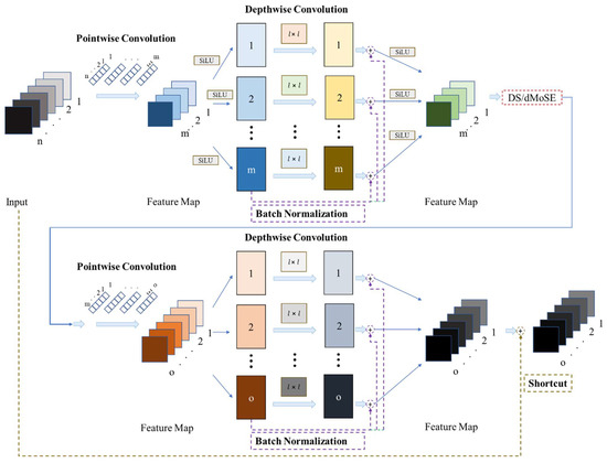
Figure 12. RepGhost bottleneck architecture.

In Figure 12, the authors of RepGhost incorporated the Squeeze-and-Excitation (SE) layer [6] into the RepGhost bottleneck module. This integration enables dynamic feature map adjustment based on input data, enhancing feature representation in convolutional neural networks. In this study, we drew inspiration from MobileNetV3 [27] and modified the SE layer by replacing its two fully connected layers with pointwise convolutions (1 × 1 Convs). This lightweight architecture, called MoSElayer, improves computational efficiency while marginally enhancing accuracy. Specifically, we replaced the activation function in the SE layer from the traditional ReLU to SiLU. These changes can allow the model to better deal with nonpositive inputs and help alleviate the gradient vanishing problem, improving feature learning and training efficiency. Moreover, the Derivative of Sigmoid Linear Unit (dSiLU) replaced the last Sigmoid function in the SE layer. This replacement could incur a slight computational overhead, contributing to higher accuracy within the architecture. The modified SE layer is termed dMoSElayer, designed to automatically focus on essential features while suppressing less relevant ones, ultimately enhancing the overall inference performance, as depicted in Figure 13. During the Squeeze phase, dMoSElayer employs global average pooling to lower the spatial dimensions of feature maps, generating a global feature descriptor. The main focus is on emphasizing critical regions within the feature maps. In the excitation phase, dMoSElayer utilizes a small gating network to amplify or suppress different feature channels selectively. The excitation triggered the model to assess how important each channel is, thereby improving its ability to capture key features like self-attention mechanism [28]. In short, dMoSElayer dynamically adjusts feature weights, allowing the model to focus more precisely on significant features while minimizing interference from irrelevant information. Finally, Figure 12 illustrates the feature extraction process in the neck and prediction stages. Additionally, the symbol “DS” denotes the down-sampling operation.

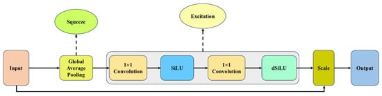
Figure 13. Derivative of Mobile Squeeze-and-Excitation Layer (dMoSE) architecture.

3.3. Dual Convolution

In Figure 14, a high-efficiency convolutional computing approach called dual convolution (Du Conv) [9] replaced some of the basic convolutional units in the proposed model, DuCRG-YOLOv11n. Similarly, the proposed DuC-ResNet18 model adopts Du Conv to replace traditional convolution layers, as shown in Figure 9. The main goal of Du Conv is to reduce computational costs while maintaining the model’s performance. In Figure 14, Du Conv comprises depthwise and pointwise convolutions. In depthwise convolution, each input feature map is processed independently with its corresponding filter (an independent 3 × 3 kernel), effectively capturing spatial details in the image. This convolution type focuses on feature interactions within a single channel. In pointwise convolution, the linear combination of the output (using an independent 1 × 1 kernel) from the previous feature maps can generate new output feature maps. Figure 14 shows how to create the intermediate feature maps as input for the subsequent layers. Finally, adding the results from these two convolutions can form the final output. The Du Conv process helps reduce computation costs because it requires fewer parameters than traditional convolution in these two steps. Moreover, since we use two different convolution kernel sizes, the model can capture features at various scales, preserving accuracy. Thus, this study applies Du Conv to construct the DuC-ResNet18 and DuCRG-YOLOv11n models. Algorithm 2 describes the detailed execution process of Du Conv.

Algorithm 2 Dual Convolution (Du Conv) [9]

$\mathrm{Input}: \mathrm{Image} X$$, \mathrm{pointwise} \mathrm{convolution} \mathrm{functions} {\mathsf{\mu }}_{h,}$ $\mathrm{Output}: \mathrm{Intrinsic} \mathrm{feature} \mathrm{map} {Outfm}_{h,g}$ Compute the output of the group convolution: Suppose that $N$ represents the number of input images, $X=\left\{x_i, \forall i=\mathrm{1,2},\dots ,N\right\}$ indicates the input images,$F=\left\{f_i, \forall i=\mathrm{1,2},\dots ,N\right\}$ denotes the depthwise filters, and $G$ stands for the number of groups. Dividing the input images $X$ into $G$ groups and the depthwise filters $F$ into $G$ groups, respectively. Execute a depthwise convolution of each input image $x_h$ once, with its corresponding filter $f_h$ by $\kappa$ ×$\kappa$ independently to attain the respective feature map ${fm}_{h,g}$, and complete a single-group convolution ${fm}_g=\{{fm}_{h,g}, \forall h=\mathrm{1,2},\dots ,N/G, g=\mathrm{1,2},\dots ,G\}$, where $N/G$ is the number of input images and respective depthwise filters for each group, the input images of a group $X_{N/G}=\left\{x_h, \forall h=\mathrm{1,2},\dots ,N/G\right\}$, and the depthwise filters of a group $F_{N/G}=\{f_h, \forall h=\mathrm{1,2},\dots ,N/G\}$. 2. Compute the output of the pointwise convolution: ${Insfm}_g={\mu }_{h,i,g}\left({fm}_h\right)={fm}_h\odot {pf}_i$ $\forall h=\mathrm{1,2},\dots ,N/G, i=\mathrm{1,2},\dots ,N/G, g=\mathrm{1,2},\dots ,G$ where ${\mathsf{\mu }}_{h,i,g}$ represents a pointwise convolution to obtain intrinsic feature maps ${Insfm}_g$, $\odot$ stands for a point-to-point product of the sum between the feature map ${fm}_h$ and pointwise filter ${pf}_i$, $N$ indicates the number of input feature maps, $G$ denotes the number of groups, and $N/G$ shows the number of input feature maps and respective pointwise filters for each group. 3. Compute the output: ${Outfm}_{h,g}={fm}_{h,g}⨁{Insfm}_g$ $\forall h=\mathrm{1,2},\dots ,N/G, g=\mathrm{1,2},\dots ,G$ $\mathrm{where} {Insfm}_g$ indicates the output feature maps, including the depthwise and pointwise convolution feature maps, ${Outfm}_{h,g}$ denotes the output feature maps in a dual convolution layer, and the symbol $⨁$ shows the pixel-wise sum of two matrixes.

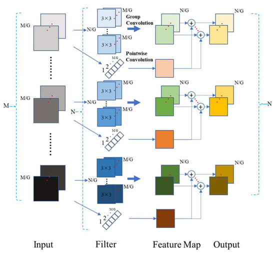
Figure 14. Dual convolution (DuConv) architecture.

Technically speaking, in our previous work [5], we performed traditional convolution operations based on specific filters to obtain the intrinsic feature maps, followed by a simple linear transformation to attain the ghost feature maps. This approach allowed us to generate the complete feature map while saving the time required for traditional convolution computing. Regarding the time complexity of various convolutions, the following shows traditional convolution, RepGhost Block, and dual convolution. O($\sum _{l=1}^u{r}_l^2·s_l^2·c_l·h_l$), O($\sum _{l=1}^u{(q_l^2·w_l^2·c_l·z_l+r}_l^2·s_l^2·z_l+t_l^2·z_l )$), and O($\sum _{l=1}^u{(r}_l^2·s_l^2·c_l+q_l^2·w_l^2·c_l·h_l)$).

We define the notation for time complexity as follows:

• $q:$ The side length of the input feature map.
• $r:$ The side length of the output feature map/the side length of the output feature map after depthwise convolution.
• $s:$ The side length of the filter/the side length of the depthwise filter.
• $c:$ The number of channels of the input feature map.
• $h:$ The number of channels of the output feature map.
• $v:$ The number of channels of a set of filters of the output feature map through a traditional convolution operation.
• $l$: An index of the convolutional layer.
• $u:$ The number of convolutional layers.
• $g:$ The number of groups in each layer.
• $t:$ The side length of the output feature map after pointwise convolution.
• $w:$ The side length of the pointwise filter.
• $z:$ The number of channels of a set of filters of the output feature map through a pointwise convolution operation.

RepGhost Block and Dual Conv’s approaches can effectively speed up the convolution computation compared to the traditional Ghost Conv. In addition, our proposed approaches can slightly increase prediction accuracy by eliminating redundant operations related to convolutional computation. By reducing the computational load and simplifying the process, these approaches let the model focus on the most relevant features, leading to faster computation and better performance in terms of accuracy.

3.4. Scenarios of Detecting Objects and Predicting Steering Angles

In Figure 15a, we installed dual cameras at the front and rear panels of a small model car, JetRacer, to capture real-time video streams, and the Jetson Nano uses DuCRG-YOLOv11n to detect moving objects and classify them. Our previous work [4] used a visual odometer to measure the distance between the detected objects and the vehicle. In Figure 15b, DuC-ResNet18 predicts the real-time steering angle along the route while the car is in motion. The predicted values led to significant changes in the steering angle, causing the vehicle to sway from side to side and oscillate violently during driving. Therefore, our previous work [4] added a PID controller to mitigate this oscillation phenomenon.

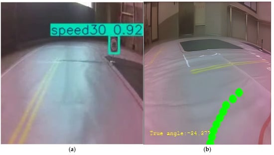
Figure 15. Live self-driving. (a) DuCRG-YOLOv11n detects objects on the road promptly, and (b) DuC-ResNet18 instantly predicts a steering angle (–34.377) with a green visual indicator on the ground.

4. Experiment Results and Discussion

This experiment initially ran a few well-known object detection models, including YOLOv8n [20], RG-YOLOv8, YOLOv11n [20], RG-YOLOv11n, and DuCRG-YOLOv11n. Next, we trailed steering angle prediction models involving VGG16 [19], ResNet18 [2], RG-ResNet18, and DuC-ResNet18. Initially, the experiment trained the DuCRG-YOLOv11n model for detecting objects and the DuC-ResNet18 model for predicting steering angles. Subsequently, we tested five detecting object models and four predicting steering angle models separately. Finally, this study combined the functions of detecting objects and predicting steering angles executing on the Jetson Nano to evaluate the performance of self-driving of the JetRacer.

4.1. Experimental Settings

Table 1 describes the hardware specification used in the experiment. Table 2 lists the software packages applied to the experiment. Table 3 shows the hardware component of the embedded platform, Jetson Nano, operating in this experiment. We used PyTorch to program the execution of deep neural networks, and ultimately, the embedded platform Jetson Nano used TensorRT to accelerate the inference.

Table 1. Hardware specification.

Unit	Component
CPU	Intel(R) Core(TM) i7-13700H CPU @ 3.60 GHz
GPU	NVIDIA GeForce GTX 4070 Ti
Memory	DDR5-5600 RAM 16 GB × 4
Storage	CT1000MX500SSD1 1TB

Table 2. Recipe of packages.

Software	Version
Python	3.8.12
Pytorch	1.9.1
Anaconda	23.7.2
JetPack	4.6
Jupyter	1.0.0

Table 3. Components of NVIDIA Jetson Nano.

Unit	Component
CPU	Quad-core ARM Cortex-A57 MPCore Processor
GPU	NVIDIA Maxwell Architecture with 128 NVIDIA CUDA® cores
Memory	4 GB 64-bit LPDDR4, 1600 MHz 25.6 GB/s
Storage	16 GB eMMC 5.1

4.2. Model Training, Inference, and Capacity

In the first stage, the training dataset collected 1476 images, and the test dataset collected 366 images, with a size of 320 × 320 for each image, to train the object detection models. The training, validation, and test data ratio was 65%, 16%, and 16%, respectively. This experiment trained all models on a GPU workstation with 300 epochs. For the test images, Equation (5) evaluates the time to infer detecting objects, where $i$ is the $i$th model, $I$ represents the number of models, $x$ stands for the $x$th image, $X$ shows the number of images, $I{T}_i$ denotes the total inference time (IT), and $EI{T}_i$ indicates the inference time of each image.

$$I{T}_i={\sum }_{x=1}^{X}EI{T}_i, where i=1, 2, \dots , I, x=1, 2,\dots , X$$

(5)

In Table 4, the first row lists the training time of each model, and the second row shows the inference time. In short, Table 4 demonstrates that DuCRG-YOLOv11n outperforms the others in both training and inference efficiency.

Table 4. Time required to train and infer detecting objects for models.

Metrics	YOLOv8n	RG-YOLOv8n	YOLOv11n	RG-YOLOv11n	DuCRG-YOLOv11n
Training (h)	1	2.3	2.0	2.8	3.0
Inference (ms)	0.8	0.9	0.9	1.1	0.7

In the second stage, the training dataset collected 14,710 images, and the test dataset collected 1000 images, with a size of 224 × 224 for each image, to train the steering angle prediction models. The data size ratio among training, validation, and test sets is the same percentage mentioned above. Similarly, Equation (5) computes the time required to predict the steering angles in the test images.

In Table 5, the first row lists the training time of each model, and the second row lists the inference time. In short, Table 5 demonstrates that DuC-ResNet18 took a bit longer than the VGG16 and ResNet18 models, while the speed of its inference was faster than the other models.

Table 5. Time to train and infer predicting steering angles for models.

Metrics	VGG16	ResNet18	RG-ResNet18	DuC-ResNet18
Training (s)	1480	2480	3245	2853
Inference (ms)	21.27	25.18	27.40	17.50

Regarding the model capacity, Table 6 lists the parameters for the object detection models, while Table 7 provides the parameters for the steering angle prediction models. YOLOv8n has the most parameters, while DuCRG-YOLOv11n has the fewest. VGG16 has the most parameters for predicting steering angles, whereas DuC-ResNet18 has the fewest parameters.

Table 6. Parameters of detecting object models.

Metrics	YOLOv8n	RG-YOLOv8n	YOLOv11n	RG-YOLOv11n	DuCRG-YOLOv11n
# of parameters	3,007,403	2,300,987	2,605,187	2,529,259	1,412,752

Table 7. Parameters of predicting steering angle models.

Metrics	VGG16	ResNet18	RG-ResNet18	DuC-ResNet18
# of parameters	14,719,938	11,177,538	11,103,490	1,447,234

4.3. Training and Validation Losses

In the experiment, visualization tools monitored the model training and callback functions executed to record the best-performing model’s parameters. After 300 training epochs, Figure 16 shows the loss curves for the best-performance detecting object model, DuCRG-YOLOv11n. The proposed model can perform better than our previous work [4]. Regarding the detection models YOLOv8n, RG-YOLOv8n, YOLOv11n, RG-YOLOv11n, and DuCRG-YOLOv11n, Figure 16, Figure 17, Figure 18, Figure 19, and Figure 20, respectively, display the training loss in the first row and the validation loss in the second row. These figures also located the localization loss, the confidence loss, and the loss of matching predicted frames to the actual frames in the first, second, and third columns. In summary, DuCRG-YOLOv11n achieved the least loss.

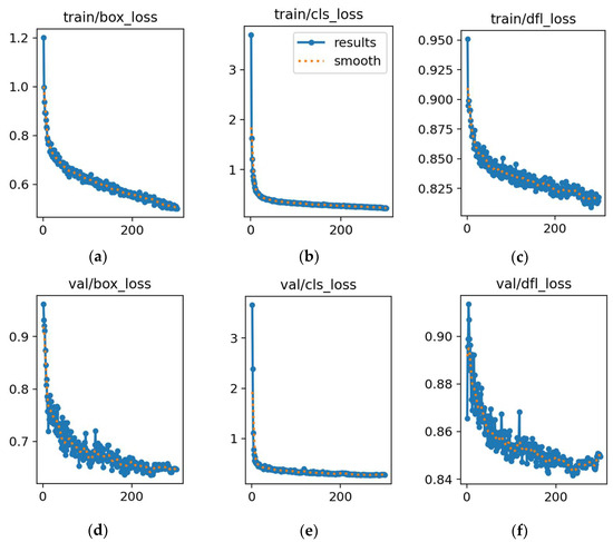
Figure 16. Training and validation losses for YOLOv8n. (a) Loss in box training. (b) Loss in classification training. (c) Loss in detection training. (d) Loss in box validation. (e) Loss in classification validation. (f) Loss in detection validation. In each plot, the x-axis represents the error value, and the y-axis represents the number of epochs.

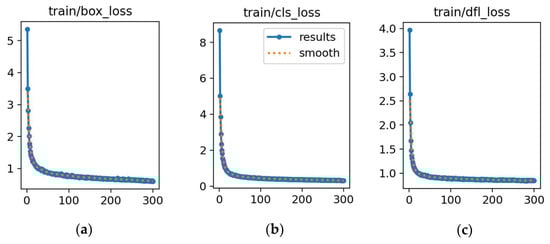
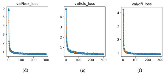
Figure 17. Training and validation losses for RG-YOLOv8n. (a) Loss in box training. (b) Loss in classification training. (c) Loss in detection training. (d) Loss in box validation. (e) Loss in classification validation. (f) Loss in detection validation. In each plot, the x-axis represents the error value, and the y-axis represents the number of epochs.

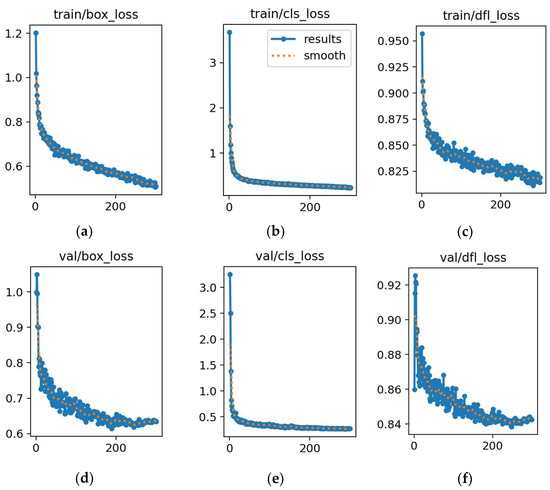
Figure 18. Training and validation losses for YOLOv11n. (a) Loss in box training. (b) Loss in classification training. (c) Loss in detection training. (d) Loss in box validation. (e) Loss in classification validation. (f) Loss in detection validation. In each plot, the x-axis represents the error value, and the y-axis represents the number of epochs.

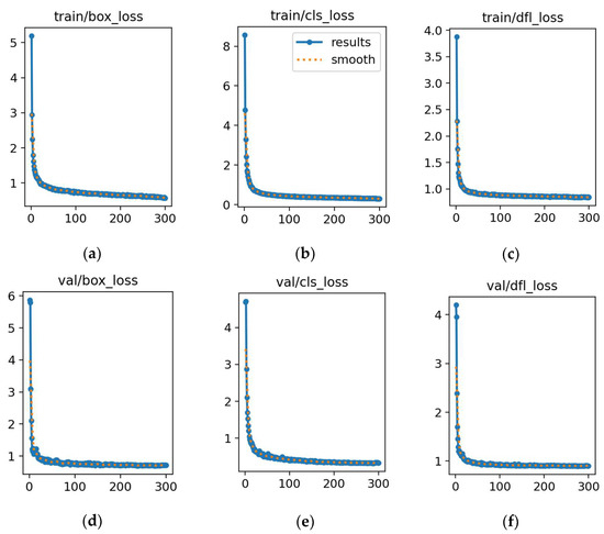
Figure 19. Training and validation losses for RG-YOLOv11n. (a) Loss in box training. (b) Loss in classification training. (c) Loss in detection training. (d) Loss in box validation. (e) Loss in classification validation. (f) Loss in detection validation. In each plot, the x-axis represents the error value, and the y-axis represents the number of epochs.

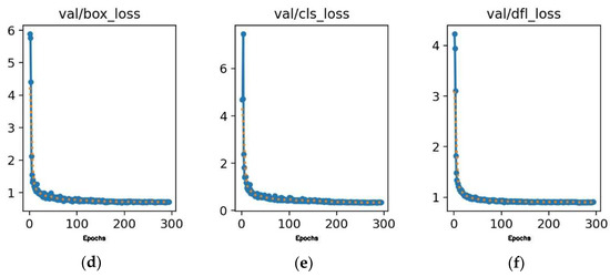
Figure 20. Training and validation losses for DuCRG-YOLOv11n. (a) Loss in box training. (b) Loss in classification training. (c) Loss in detection training. (d) Loss in box validation. (e) Loss in classification validation. (f) Loss in detection validation. In each plot, the x-axis represents the error value, and the y-axis represents the number of epochs.

After 200 training epochs, Figure 21 shows the loss curves for the best-performance predicting steering angle model, DuC-ResNet18. The proposed model can perform better than our previous work [4]. Figure 20 displays the training and validation losses in blue and red. DuC-ResNet18 reduced the validation loss to 0.0513.

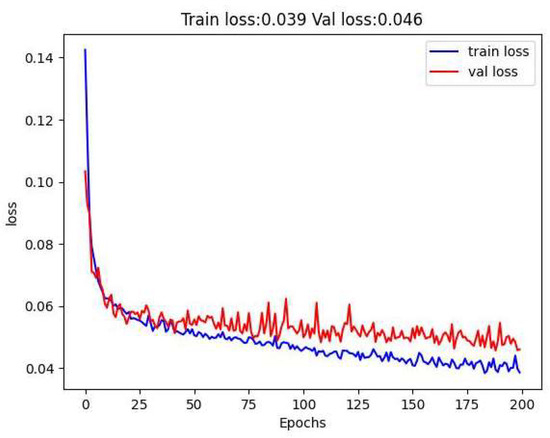
Figure 21. Losses in training and validation for DuC-ResNet18.

4.4. Model Testing

Equation (6) evaluates how many frames are executed detecting in a second (frames per second, FPS), where $J$ is the number of applied models, $FP{S}_j$ implies the frames per second of the $j$th model, and ${IRAIT}_j$ denotes the time taken to instantly detect an object using the $j$th model.

$$FP{S}_j={\displaystyle \frac{1}{{IRAIT}_j}}, where j=1, 2,\dots , J$$

(6)

A given model can compute the detection precision (mean average precision, mAP) to indicate object detection, and the user can retrieve this value by the mean of every class’s average precision for all classes. Equation (7) evaluates the detection precision of every model to detect objects $mA{P}_l$, where $L$ is the number of applied models, $k_l$ implies a designated class in the $l$th model, $C_l$ means the number of designated classes in the $l$th model,$mA{P}_l$ indicates the detection precision of the $l$th model, and ${AP}_{k_l}$ denotes the detection precision of a designated class in the $l$th model.

$$mA{P}_l={\displaystyle \frac{{\sum }_{k_l=1}^{C_l}{AP}_{k_l}}{C_l}}, where k_l=1, 2, \dots , C_l, l=\mathrm{1,2},\dots ,L$$

(7)

The experiment detected objects on 366 test images and estimated the speed and accuracy of each object detection model. Figure 22 shows the precision–recall curve and indicates each dot’s specific recall and precision. In Figure 22, the x-axis implies recall, and the y-axis denotes precision. The experiment tested the results of the following models: YOLOv8n, RG-YOLOv8n, YOLOv11n, RG-YOLOv11n, and DuCRG-YOLOv11n. Equation (6) calculates the FPS, and Equation (7) calculates the mAP, as listed in Table 8. To summarize this test, DuCRG-YOLOv11n achieved the best results, while YOLOv8n performed the worst.

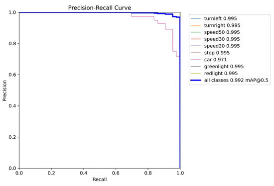
Figure 22. Precision–recall curve for DuCRG-YOLOv11n.

Table 8. Speed and precision of detecting objects.

Metrics	YOLOv8n	RG-YOLOv8n	YOLOv11n	RG-YOLOv11n	DuCRG-YOLOv11n
FPS	125	129	128	131	147
Precision (%)	97.1	97.5	99.0	99.2	99.1

Likewise, Equation (6) computes how many frames are executed in predicting in a second (frames per second, FPS). Equation (8) computes the error (mean square error, $MSE$) of predicting steering angles, where $MSE$ is the accuracy of a prediction model, $N$ denotes the number of input images, $k$ means the $k$th image, $y_i$ implies the actual outcome, and ${\widehat{y}}_i$ indicates the predicted outcome. The smallest MSE represents the beat accuracy of predicting the steering angle.

$$MSE={\displaystyle \frac{\sum _{k=1}^N{(y_k-{\widehat{y}}_k)}^2}{N}}, \mathrm{w}\mathrm{h}\mathrm{e}\mathrm{r}\mathrm{e} k=\mathrm{1,2},\dots , N$$

(8)

Predicting the steering angles on 1000 testing images can estimate the detection speed and then evaluate the accuracy of angle prediction for each model. In Figure 23, the curves show the predicted values versus the actual values for steering angle prediction model DuC-ResNet18. Figure 23 indicates “−1” as a right turn, implies “1” as a left turn, and denotes “0” as going straight, where the scale for the turning points ranges from −1 to 1 for the steering angle. The proposed model can perform better than our previous work [4]. Equation (6) calculates FPS, and Equation (8) calculates MSE, as shown in Table 9. This test indicates that RG-ResNet18 achieved the smallest MSE, while VGG16 performed the worst.

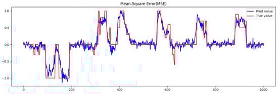
Figure 23. The MSE of predicted and actual steering angle using Du-ResNet18.

Table 9. Speed and loss of predicting steering angles.

Metrics	VGG16	ResNet18	RG-ResNet18	DuC-ResNet18
FPS	31.9	27.0	48.34	57.13
MSE	0.0849	0.0712	0.0019	0.0587

4.5. Performance Evaluation

Jetson Nano executes the self-driving control using the frame per second (FPS) and mean square error (MSE) to evaluate metrics. When the JetRacer travels along the route map, the NVIDIA JetRacer instantly detects objects and simultaneously predicts the steering angle. Self-driving may take longer to detect objects or lack the time needed to predict steering angles, which may endanger the car’s safety in unexpected situations. Therefore, the frame rate could be the most crucial consideration of risk. Jetson Nano can accelerate the detection of objects using TensorRT, ensuring a faster and more efficient self-driving system.

Equation (6) calculates the frame rate for different combinations when the video resolution is 320 × 320, as shown in Table 10. In Table 10, DuCRG-YOLOv11n consistently achieves the best speed across various combinations. The combination of DuCRG-YOLOv11n and DuC-ResNet18 achieves the best FPS, while YOLOv8n and VGG16 result in the lowest FPS.

Table 10. FPS of model combination.

	O. D.	YOLOv8n	RG-YOLOv8n	YOLOv11n	RG-YOLOv11n	DuCRG-YOLOv11n
St. A. P.
VGG16		25.4	25.6	25.5	25.7	25.9
ResNet18		37.1	37.4	37.3	37.6	37.8
RG-ResNet18		38.6	42.1	40.0	43.8	44.5
DuC-ResNet18		43.1	48.6	44.7	49.6	50.7
Average		36.0	38.4	36.8	39.0	39.72

Note: O. D. represents object detection; St. A. P. represents steering angle prediction.

Subsequently, the experiment evaluated the accuracy of detecting objects and then the accuracy of predicting steering angles for each combination, with the video resolution set to 320 × 320. Equation (7) computes the accuracy of object detection, and Equation (8) calculates the accuracy of steering angle prediction. In Table 11, RG-YOLOv11n achieves the best detection accuracy, while RG-ResNet18 has the lowest MSE for predicting steering angles.

Table 11. Accuracy and precision of model combination.

	Precision(%)	O. D.
MSE		YOLOv8n	RG-YOLOv8n	YOLOv11n	RG-YOLOv11n	DuCRG-YOLOv11n
St. A. P.	VGG16	(0.0849, 97.1)	(0.0849, 97.5)	(0.0849, 99.0)	(0.0849, 99.2)	(0.0849, 99.1)
	Resnet18	(0.0712, 97.1)	(0.0712, 97.5)	(0.0712, 99.0)	(0.0712, 99.2)	(0.0712, 99.1)
	RG-ResNet18	(0.0019, 97.1)	(0.0019, 97.5)	(0.0019, 99.0)	(0.0019, 99.2)	(0.0019, 99.1)
	DuC-ResNet18	(0.0578, 97.1)	(0.0578, 97.5)	(0.0578, 99.0)	(0.0578, 99.2)	(0.0578, 99.1)

Note: O. D. represents object detection; St. A. P. represents steering angle prediction.

4.6. Discussion

Carrasco et al. [13] proposed YOLOv5_SM_x2, which achieves an average precision (mAP) of 0.998 at 42.82 frames per second (FPS). While this model demonstrates impressive precision, it fails to meet the Level 4 (L4) safety requirements for self-driving when applied in this study. Wei et al. [27] combined millimeter-wave and visual detection, but this information fusion could waste a significant amount of time, slowing down object detection speeds. Y. Cai et al. [29] conducted experiments using an NVIDIA GTX 2080Ti as the computing engine, detecting objects at 66 FPS. However, since the Jetson Nano’s graphics processing speed is significantly slower than that of the NVIDIA GTX 2080Ti, it fails to achieve safe self-driving performance. In previous work, Chang et al. [4] proposed LWGSE-YOLOv4-tiny to implement fast object detection and LWDSG-ResNet18 to realize quick steering angle prediction, achieving 56.1 FPS in object detection and a mean square error of around 0.0683 for steering angle prediction. However, after data fusion, the FPS dropped to 24.9, and the slower processing speed could lead to serious accidents at high speeds. Despite this, the proposed self-driving vision algorithms in this study can speed up the computing in Jetson Nano, achieving 147 FPS for rapid object detection. Our proposed approaches can detect objects simultaneously and accurately predict steering angles.

Predicting delayed steering angles can significantly increase the number of dangerous unexpected events. The fast detection and response are much more important than precision in such scenarios. Two models, YOLOv11n and ResNet18, were improved by introducing the modification ones, DuCRG-YOLOv11n and DuC-ResNet18, accelerating detection speed while escalating image recognition accuracy. As a result, compared to YOLOv11n, DuCRG-YOLOv11n increased the feature extraction frame rate by 14.84% and slightly improved the accuracy of detecting objects by 0.1%. Compared with ResNet18, DuC-ResNet18 achieved a 111.59% increase in prediction speed and a 23.18% improvement in image recognition accuracy. Therefore, the proposed methods fulfill the main objective of this study.

Unfortunately, the experiment found shortcomings in this scenario. Jetson Nano encounters hardware limitations. Jetson Nano cannot handle real-time, high-resolution video streams while the model car moves. Instead of Jetson Nano, Jetson Orin Nano is a good choice for fast capture and complete processing of higher-resolution video streams. Unfortunately, despite Jetson Orin Nano having a lower power consumption than Jetson AGX Xavier, it still cannot provide a sufficient battery life for the JetRacer. Therefore, an energy-efficient model vehicle is required to address this limitation.

5. Conclusions

This study contributes to the realization of high-speed control response for object detection integrated with steering angle prediction, meeting the requirements for L4 safety in self-driving. DuCRG-YOLOv11n significantly promotes the speed of object detection. Meanwhile, DuC-ResNet18 substantially escalates the speed of steering angle prediction. As a result, the proposed approaches can reduce the overall reaction time for self-driving responses. Technically, the proposed method enables high-speed execution of self-driving control and effectively achieves the goal of L4 safe self-driving. The proposed approaches significantly beat our previous work [4] in increasing the overall speed of self-driving control by 2.04 times. According to the performance comparison, the proposed approaches outperform the other alternative methods.

In the future, we will continue to pursue ways to improve object detection and predict steering angles to meet the requirements for L5 safety in self-driving. Furthermore, integrating high-speed vision algorithms into in-vehicle supercomputers is a key part of the future trend in self-driving. Therefore, combining the Robot Operating System (ROS) with high-speed vision algorithm inference to control self-driving cars will also be a significant issue moving forward. We aim to find low-power, high-performance embedded platforms to run these high-speed vision algorithms. This solution enables a cost-effective and efficient edge computing architecture for the safe and smooth operation of self-driving cars.

References

- Wang, C.Y.; Bochkovskiy, A.; Liao, H.Y.M. Scaled-YOLOv4: Scaling Cross Stage Partial Network. In Proceedings of the IEEE/CVF Conference on Computer Vision and Pattern Recognition, Nashville, TN, USA, 20–25 June 2021; pp. 13029–13038. [Google Scholar]
- He, K.; Zhang, X.; Ren, S.; Sun, J. Deep Residual Learning for Image Recognition. In Proceedings of the IEEE/CVF Conference on Computer Vision and Pattern Recognition, Las Vegas, NV, USA, 27–30 June 2016; pp. 770–778. [Google Scholar]
- Chang, B.R.; Tsai, H.F.; Chou, H.L. Accelerating the response of self-driving control by using rapid object detection and steering angle prediction. Electronics 2023, 12, 2161. [Google Scholar] [CrossRef]
- Chang, B.R.; Tsai, H.F.; Chang, F.Y. Boosting the response of object detection and steering angle prediction for self-driving control. Electronics 2023, 12, 4281. [Google Scholar] [CrossRef]
- Han, K.; Wang, Y.; Tian, Q.; Guo, J.; Xu, C.; Xu, C. GhostNet: More features from cheap operations. In Proceedings of the IEEE/CVF Conference on Computer Vision and Pattern Recognition, Seattle, WA, USA, 13–20 June 2020; pp. 1580–1589. [Google Scholar]
- Hu, J.; Shen, L.; Sun, G. Squeeze-and-excitation networks. In Proceedings of the IEEE/CVF Conference on Computer Vision and Pattern Recognition, Salt Lake City, UT, USA, 18–23 June 2018; pp. 7132–7141. [Google Scholar]
- Howard, A.; Sandler, M.; Chu, G.; Chen, L.-C.; Chen, B.; Tan, M.; Wang, W.; Zhu, Y.; Pang, R.; Vasudevan, V.; et al. Searching for MobileNetV3. In Proceedings of the IEEE/CVF International Conference on Computer Vision (ICCV), Seoul, Republic of Korea, 27 October–2 November 2019; pp. 1314–1324. [Google Scholar] [CrossRef]
- Chen, C.; Guo, Z.; Zeng, H.; Xiong, P.; Dong, J. RepGhost: A hardware-efficient ghost module via reparameterization. arXiv 2022, arXiv:2211.06088. [Google Scholar] [CrossRef]
- Zhong, J.; Chen, J.; Mian, A. DualConv: Dual convolutional kernels for lightweight deep neural networks. IEEE Trans. Neural Netw. Learn. Syst. 2022, 33, 1904–1918. [Google Scholar] [CrossRef] [PubMed]
- Li, S.; Zhang, Y.; Blythe, P.; Edwards, S.; Ji, Y. Remote driving as the Failsafe: Qualitative investigation of Users’ perceptions and requirements towards the 5G-enabled Level 4 automated vehicles. Transp. Res. F: Traffic Psychol. Behav. 2024, 100, 211–230. [Google Scholar] [CrossRef]
- JetRacer AI Kit. Waveshare Wiki. 2023. Available online: https://www.waveshare.com/wiki/JetRacer_AI_Kit (accessed on 1 March 2025).
- Dong, X.; Yan, S.; Duan, C. A lightweight vehicle detection network model based on YOLOv5. Eng. Appl. Artif. Intell. 2022, 113, 104914. [Google Scholar] [CrossRef]
- Carrasco, D.P.; Sotelo, M.A.; Rodríguez, F.J. T-YOLO: Tiny vehicle detection based on YOLO and multi-scale convolutional neural networks. IEEE Trans. Intell. Transp. Syst. 2022, 23, 4906–4915. [Google Scholar]
- Momin, M.A.; Junos, M.H.; Khairuddin, A.S.M.; Talip, M.S.A. Lightweight CNN model: Automated vehicle detection in aerial images. Signal Image Video Process 2023, 17, 1209–1217. [Google Scholar] [CrossRef]
- Cai, D.; Li, K.; Hou, B. YOLOv8-RepGhostEMA: An efficient underwater trash detection model. J. Phys. Conf. Ser. 2024, 2906, 012019. [Google Scholar] [CrossRef]
- Wang, H.; Liu, C.; Cai, Y.; Chen, L.; Li, Y. YOLOv8-QSD: An improved small object detection algorithm for autonomous vehicles based on YOLOv8. IEEE Trans. Instrum. Meas. 2024, 73, 1–16. [Google Scholar] [CrossRef]
- Rambus. Driving Automation Levels. Rambus Blog. 2023. Available online: https://www.rambus.com/blogs/driving-automation-levels/ (accessed on 8 January 2025).
- Australian Parliament House. Inquiry into The Impact of New and Emerging Technologies on The Australian Economy. Parliament of Australia. 2023. Available online: https://www.aph.gov.au/DocumentStore.ashx?id=bb8568ee-b1c1-4f47-adb2-dc2b73eaa6c4&subId=304019 (accessed on 16 January 2025).
- He, K.; Zhang, X.; Ren, S.; Sun, J. Delving deep into rectifiers: Surpassing human-level performance on ImageNet classification. arXiv 2014, arXiv:1409.1556. [Google Scholar] [CrossRef]
- Ultralytics. GitHub. 2023. Available online: https://github.com/ultralytics/ultralytics (accessed on 20 November 2024).
- Wang, C.-Y.; Bochkovskiy, A.; Liao, H.-Y.M. YOLOv7: Trainable bag-of-freebies sets new state-of-the-art for real-time object detectors. arXiv 2022, arXiv:2207.02696. [Google Scholar] [CrossRef]
- Lin, T.-Y.; Dollar, P.; Girshick, R.; He, K.; Hariharan, B.; Belongie, S. Feature Pyramid Networks for Object Detection. In Proceedings of the IEEE Conference on Computer Vision and Pattern Recognition (CVPR), Honolulu, HI, USA, 21–26 July 2017; pp. 2117–2125. Available online: https://openaccess.thecvf.com/content_cvpr_2017/html/Lin_Feature_Pyramid_Networks_CVPR_2017_paper.html (accessed on 30 November 2024).
- Sapkota, R.; Meng, Z.; Churuvija, M.; Du, X.; Ma, Z.; Karkee, M. Comprehensive performance evaluation of YOLOv12, YOLO11, YOLOv10, YOLOv9, and YOLOv8 on detecting and counting fruitlet in complex orchard environments. arXiv 2024, arXiv:2407.12040. [Google Scholar] [CrossRef]
- Liu, H.; Liu, F.; Fan, X.; Huang, D. Polarized Self-Attention: Towards High-Quality Pixel-Wise Regression. arXiv 2021, arXiv:2107.00782. [Google Scholar] [CrossRef]
- Khanam, R.; Hussain, M. YOLOv11: An Overview of the Key Architectural Enhancements. arXiv 2024, arXiv:2410.17725. [Google Scholar] [CrossRef]
- Klambauer, G.; Unterthiner, T.; Mayr, A.; Hochreiter, S. Self-Normalizing Neural Networks. In Proceedings of the 31st International Conference on Neural Information Processing Systems, Long Beach, CA, USA, 4–9 December 2017; pp. 972–981. [Google Scholar]
- Wei, Z.; Zhang, F.; Chang, S.; Liu, Y.; Wu, H.; Feng, Z. mmWave Radar and Vision Fusion for Object Detection in Autonomous Driving: A Review. Sensors 2022, 22, 2542. [Google Scholar] [CrossRef]
- Liu, Y.; Ma, L.; Liu, Y.; Zhang, Y.; Yang, M. SA-YOLOv3: An efficient and accurate object detector using self-attention mechanism for autonomous driving. IEEE Trans. Intell. Transp. Syst. 2020, 23, 2326–2330. [Google Scholar]
- Cai, Y.; Luan, T.; Gao, H.; Wang, H.; Chen, L.; Li, Y.; Sotelo, M.A.; Li, Z. YOLOv4-5D: An Effective and Efficient Object Detector for Autonomous Driving. IEEE Trans. Instrum. Meas. 2021, 70, 4503613. [Google Scholar] [CrossRef]
Disclaimer/Publisher’s Note: The statements, opinions and data contained in all publications are solely those of the individual author(s) and contributor(s) and not of MDPI and/or the editor(s). MDPI and/or the editor(s) disclaim responsibility for any injury to people or property resulting from any ideas, methods, instructions or products referred to in the content. |
© 2025 by the authors. Licensee MDPI, Basel, Switzerland. This article is an open access article distributed under the terms and conditions of the Creative Commons Attribution (CC BY) license (https://creativecommons.org/licenses/by/4.0/).