Abstract
A cyber–physical multi-robot system integrates robotic agents that share data over communication networks in real time to achieve common objectives by making decisions collectively based on the knowledge of their surroundings. This work introduces a formation control strategy for two groups of mobile robots placed in two separate workspaces connected by a communication network. The control technique generates two similar formations on each workspace using virtual agents that mirror the behavior of the corresponding physical robot in the opposite workspace. Control laws are derived for a single integrator and unicycle-type real and virtual robots that converge to the desired formation, even in the presence of communication delays. The numerical simulations performed show the convergence of the control strategy. A low-cost cyber–physical micro-robot platform was developed to run experiments with real robots. The setup uses a camera as a position and orientation sensor and the MQTT protocol for server communication and data exchange. Results obtained on this platform show the feasibility of the approach in an actual physical setting.
1. Introduction
The control and coordination of multiple mobile robots [1] is an important research area for current technological advances in the use of industrial and service robots [2]. In recent years, the use of mobile agents in logistics [3], health [4], field [5], and military defense tasks robots [6] has increased [7].
The problem formulation in mobile robotics is initially addressed with respect to the kinematic model of the mobile robot type and mechanical configuration. Some contributions have been addressed for differential-drive or unicycle-type wheeled robots [8], omnidirectional robots [9] and car-like configurations. In addition to the individual control of mobile robots, it is possible to coordinate a group of robots for logistics and transportation tasks [10,11]. The fundamental problems in the coordination of mobile robots are formation control [12], formation tracking or marching control [13], and inter-robot collision avoidance [14,15,16].
The cyber–physical formation schemes are a recent focus for the multi-robot control community. These schemes include the strategies to coordinate mobile robots moving in different physical workspaces, sharing information through the internet and the cloud [17]. This new formation scheme is possible thanks to wireless communication devices with high bandwidth [18] and embedded robust computing architectures [19], which allow formation control laws that could be executed onboard the robots themselves or in the cloud. In these cyber–physical systems, the robots can achieve coordinated motion across remote workspaces.
Communication delays have an effect on cyber–physical systems workspaces, which can significantly affect their performance if they are not addressed properly. Predictor-based methods have been extensively used to estimate future states and compensate for delays [20]. Stability analysis has employed Lyapunov–Razumikin and Lyapunov–Krasovski functionals, leading to linear matrix inequality conditions that can be efficiently solved [21,22], which can handle multiple and variable delays and reach tighter conditions [23]. Other approaches include passivity-based [24], back-stepping, and sliding-mode control [25], among others.
Recent advances in cyber–physical formation schemes are shown [26] that propose a hierarchical scheduling strategy for mobile robots in multi-warehouse environments, integrating industrial cyber–physical systems to optimize logistics operations. Ref. [27] presents a cyber–physical control system designed for autonomous logistic robots, focusing on real-time decision-making and integration with industrial automation platforms. Ref. [28], introduces a cyber–physical system for optimal trajectory planning of mobile robots, explicitly considering the deterioration of electric motors to improve long-term performance and energy efficiency.
The main issues in this scheme across different workspaces are sharing information through the internet [29,30], new challenges for control schemes [31,32,33], delay effects in internet communications [34,35], the problem of communication losses between workspaces [36,37], and the impact of intermittent connectivity on internet links [38,39,40].
This work includes the development of a low-cost platform of a multi-robot system with a cyber–physical connection. Some multi-robot platforms for educational purposes are based on the development of omnidirectional robots [41,42], cooperative task systems [30], and cyber–physical [17].
This article presents an extension of our previous work [43] , including detailed proofs handling communication delays and adding new experiments to show the robustness of the theoretical results presented. The main contributions are as follows.
- The design and implementation of a control strategy for a cyber–physical formation of mobile robot systems moving in two workspaces. The control approach is based on the use of virtual agents that converge with the physical robots moving in the opposite workspace. The convergence is analyzed for the general case of n robots. Under this control scheme, the robots behave as if they move in a unique workspace.
- The problem formulation is established for single integrator robots in . However, it has a broader scope since it is known that different nonholonomic mobile robots can be reduced to this simple representation using an appropriate input–output linearization transformation.
- The control approach is developed for 2D single integrator robots, but it is extended to unicycle-type robots with two wheels, and it is validated by numerical simulations.
- Finally, a low-cost experimental platform is built. An experiment is shown using four robots in two different physical spaces communicated through an internet connection with an MQTT protocol, different formation topologies, sample rates, and MQTT brokers are tested.
The paper is organized as follows. The problem definition is given in Section 2. The control strategy is presented in the Section 3. Numerical simulations are shown in Section 4. The experimental platform is introduced and its results are reported in Section 5. Finally, concluding remarks and future research directions are drawn in Section 6.
2. Problem Formulation
In this work, the cyber–physical formation problem is defined for n point-robots moving in two different workspaces.
Let be a set of mobile planar robots moving in two different workspaces and . Without loss of generality, assume that and , with , are the subsets of robots moving in and , respectively. Therefore, with . Define as the 2D position of in or .
This work is focused on the construction of a leader–follower formation control strategy such that the robots in the two workspaces converge to a global formation as if they were in the same space. The leader robot should follow a desired trajectory given by .
A desired global formation graph for the n robots is given by an adjacency matrix , a set of relative positions , and a Laplacian matrix . The challenge in a cyber–physical configuration is to converge to the formation specified by in the absence of certain robots in each workspace. To carry this out, the information about the positions , must be shared between and , as illustrated in Figure 1 using the internet and the cloud.
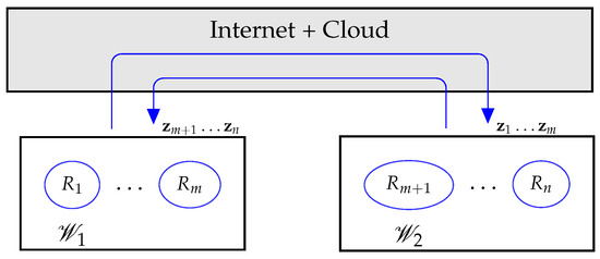
Figure 1.
Communication between workspaces and .
3. Control Strategy
To tackle the cyber–physical formation problem defined in the previous section, this work proposes the use of virtual robots. Thus, for each , , define a virtual robot , , and for each , , define a virtual robot , . Thus, there are also n virtual robots divided into and . Let be the 2D position of each virtual robot . Finally, and .
For this new cyber–physical system composed of agents generated in this way, a combined formation graph , derived from , is defined as follows.
For each , let and be the adjacent subsets of the indexes of the real and virtual robots in that are communicated to according to the following:
In addition, all virtual robots are communicated only to their real counterparts located in the other workspace ; i.e., their corresponding adjacent subsets are
An example of such a communication topology is shown in Figure 2. Furthermore, for each with , let the desired static and predefined relative position vector be with . By design, it is straightforward to show that if has a directed spanning tree, then also has one. Having a directed spanning tree, it is well known that the Laplacian matrix of and , given by and respectively, have exactly one zero eigenvalue, the rest being positive [1].
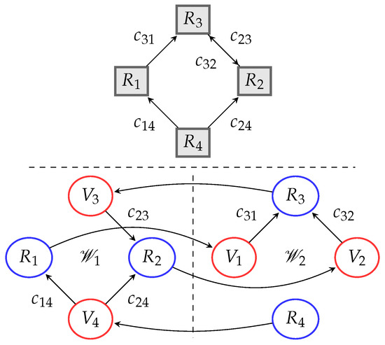
Figure 2.
An example for of the relationship between the original formation graph (above) and workspaces and and combined graph (below).
In the following, the control laws for this configuration of real and virtual robots are defined. First, consider both real and virtual robots as single integrators, given by
where and are the control inputs for the real and virtual robots, respectively. For the leader–follower control strategy introduced in this work, let us define as the leader robot and , as the desired position and velocity of the trajectory for the leader. Furthermore, workspaces and could be a long distance away from each other, and therefore, a sizable delay should have to be taken into account on the information passed between them.
The control strategy for the virtual robots is designed to track its corresponding real robot that belongs to the other workspace , according to the following law:
where is the communication delay between workspaces, and is the control gain for the virtual robots. The control law for the real robots is given by the following:
with being the control gain for the real robots and . The control strategy for the leader robot is given by
where the control gain . Note that the control law for the real robots is not affected by the communication delay between the workspaces, since all required information is within its own workspace. Defining the relative positions of the robots with respect to the desired trajectory and , Equations (4)–(6) have a relative equilibrium formation defined by
Let and be the relative error with respect to the formation trajectory of the real and virtual robots, respectively. Using the above equations, the error dynamics can be expressed as
where
with being a zero vector of dimension k.
3.1. Without Communication Delays
In an ideal case in which there are no delays in the information carried out between workspaces, we can state the following result.
Theorem 1.
For a set of n mobile robots distributed over two physical workspaces and with first-order dynamics given by Equation (3) and a leader–follower formation setup given by a communication topology derived from the original topology with a directed spanning tree and defined by (1), (2), the control strategy given by Equations (4)–(6) without delay () reaches convergence of the error dynamics (10) to the origin, achieving the relative formation defined by Equation (7).
Proof.
When there is no communication delay, i.e., , the error dynamics (8) can be simplified to
In order to prove the convergence of dynamics (10), it is sufficient to show that all the eigenvalues of the matrix have a negative real part. Note that
with . Since , where all the diagonal elements , by applying the Gershgorin Circle’s Theorem and taking into account the structure of the Laplacian matrix, it is straightforward to see that the matrix may have one zero eigenvalue while the rest have a negative real part. Since , , , and are all positive, the same can be said of . To complete the proof, it will be shown that does not have a zero eigenvalue.
For to have a zero eigenvalue, there must exist a non-null vector such that . Using expression (11) and writing
Because of the assumption that has a directed spanning tree, has a single zero eigenvalue. Thus, its LU decomposition has the following structure:
where is a lower triangular matrix with its main diagonal elements equal to 1 and matrix is an upper triangular matrix with its main diagonal elements , and . Observe that is invertible and also . Substituting (13) into (12) gives
Since , and , the only solution of Equation (14) is . Therefore, the only solution to Equation (12) is also , which implies that and do not have a zero eigenvalue. Consequently, the error dynamics (10) are stable. □
3.2. With Communication Delays
When a delay in communication between workspaces cannot be neglected, delayed dynamics (8) must be analyzed. The next result looks at conditions to have stability of the closed loop in the event of having communication delays.
Theorem 2.
For a set of n mobile robots distributed over two physical workspaces and with first-order dynamics given by Equation (3) and a leader–followers formation setup given by a communication topology with unknown fixed bounded delay () and a control strategy given by Equations (4)–(6), if there exist symmetric positive definite matrices , , such that
with
the closed loop error dynamics (8) reaches convergence to the origin, achieving relative formation defined by Equation (7).
It should be noted that Equation (15) constitutes a Linear Matrix Inequality (LMI) in the coefficients of the matrices and parameterizable in T.
Proof.
Let describe the error vector at time t. Let us also define as the error trajectory in the delay interval . The error dynamics (8) can be rewritten as
with matrices and given by (16). In order to prove the stability of (17), we define a Lyapunov–Krasovski functional by the following expression:
Choosing matrices and symmetric and positive definite makes the functional V positive definite as well. Taking the time derivative of (18) and applying Jensen’s inequality, we obtain
Let us define the vector . Substituting Equations (17), (15) and (16) into (19) and rearranging terms, we obtain
If the LMI given by (15) is satisfied, the time derivative of the Lyapunov–Krasovski functional along the trajectories will be negative, and the error dynamics will converge to the origin, making the cyberphysical system converge to the desired formation pattern in workspaces and . □
Remark 1.
The LMI condition here is conservative, since the last term of can be further developed using tighter inequalities to obtain a closer LMI condition.
Remark 2.
Since the LMI condition depends on T but not explicitly on τ, if there is a solution to (15), the stability can be ensured for any .
Remark 3.
It is fairly straightforward to extend this result to multiple delays and time varying delays with bounds on the time derivative of the delay function, arriving at one or several LMI conditions like (15).
Remark 4.
There are efficient computational methods and tools to solve LMIs. In this work, the YALMIP toolbox for Matlab with the Gurobi optimizer has been used to check the condition in the experiments shown in the following sections.
4. Numerical Simulations
For the numerical simulation, a Python 3.13 code was developed using Matplotlib and NumPy libraries to simulate various trajectories and robot formations within two distinct workspaces. Three formations were implemented: the first consists of two robots arranged in a straight line (one per workspace, as shown in Figure 3); the second consists of four robots arranged in a straight line (two per workspace, as depicted in Figure 4); and the third consists of four robots arranged in a diamond configuration (two per workspace, as illustrated in Figure 5). In each formation, a leader robot maintains a circular trajectory. The formations were evaluated using different gain parameters (, , and ), as well as various delay values in the virtual robots’ data. Simulation errors were quantified through comparative tables based on the norm (integral of the sum of absolute errors) and the norm (integral of the sum of squared errors).
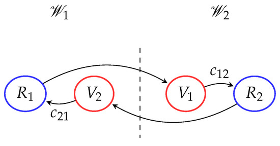
Figure 3.
First formation topology: 2-robot horizontal line shape formation.
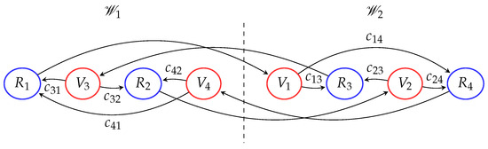
Figure 4.
Second formation topology: 4-robot horizontal line shape formation.
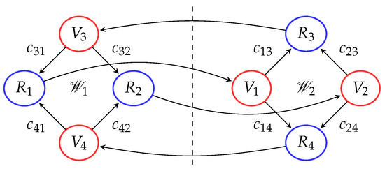
Figure 5.
Third formation topology: 4 Diamond shape robots.
4.1. Without Communication Delays
Figure 6 shows the numerical simulation of the control approach with , and ; the total number of robots is , where and , based on the workspace and topology formation, as shown in Figure 3. The leader robot is . Therefore, and , and the total members of each workspace are and .
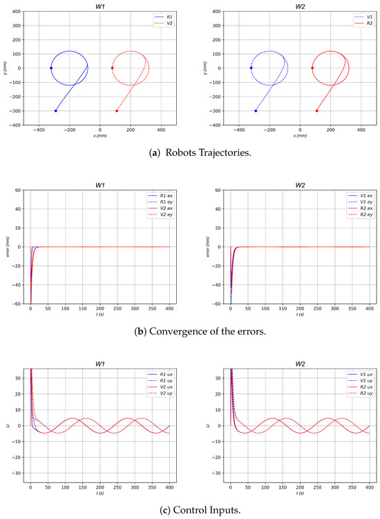
Figure 6.
Numerical simulation for a 2-Robots horizontal line shape formation.
The adjacent subsets for the real robots are defined as , , , , as shown in Figure 3. The desired final formation of the robots is a horizontal line, as if both real robots were in the same workspace. To achieve this desired formation pattern, the relative vectors are given by , with and by construction .
Figure 6a shows the trajectories of the real and virtual robots using the control law (4)–(5)–(6) with , , and the desired trajectory of the leader robot given by . All robots converge to the desired horizontal line formation pattern, which is observed by the convergence of the errors as shown in Figure 6b, and the control inputs are observed in Figure 6c.
In the first formation, shown in Figure 3, several simulations were conducted by varying the values of , , and to demonstrate the stability and convergence speed of the control strategy. Simulations were performed using k values of , 1, and 10, as well as their various combinations, while ensuring that remained greater than or equal to and . For each simulation, the and norms were computed by summing the absolute errors and the squared errors, respectively, taking into account errors from both workspaces, real and virtual robots. The results are depicted in the graphs in Figure 7 and summarized in Table 1.
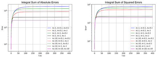
Figure 7.
and norms with different k values in the simulation of 2-robot horizontal line shape formation.

Table 1.
and norms for different k values in the simulation of 2-robot horizontal line shape formation.
The second formation topology, as shown in the Figure 8, shows the numerical simulation of the control approach with , and , i.e., the total set of robots is , where and , based on the workspace and topology formation, as shown in Figure 4. The leader robot is . Therefore, and and the total members of each workspace are and .
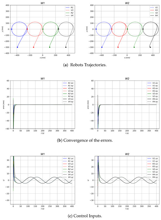
Figure 8.
Numerical simulation of 4-robot horizontal line shape formation.
The adjacent subsets for the real robots are defined as , , , , , , , , as shown in Figure 4. The desired final posture of the robots is a horizontal line formation, as if all four real robots would be in the same workspace. To achieve this desired formation pattern, the relative vectors are given by , , , , with and by construction , , and .
Figure 8a shows the trajectories of the real and virtual robots using the control law (4)–(5)–(6) and again with , , and the desired trajectory of the leader robot given by . All robots converge to the desired horizontal line formation pattern, which is observed by the error convergence shown in Figure 8b, and the control inputs are observed in the Figure 8c.
In the second formation, shown in Figure 4, several simulations were conducted by varying the values of , , and to demonstrate the stability and convergence speed of the control strategy. Simulations were performed using k values of , 1, and 10, as well as their various combinations, while ensuring that remained greater than or equal to and . For each simulation, the and norms were computed by summing the absolute errors and the squared errors, respectively, taking into account errors from both workspaces, real and virtual robots. The results are depicted in the graphs in Figure 9 and summarized in Table 2.
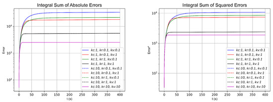
Figure 9.
and norms with different k values in simulation of 4-robot horizontal line shape formation.
Table 2.
and norms for different k values in the simulation of 4-robot horizontal line shape formation.
The third formation topology for numerical simulation, as shown in Figure 10, presents the control approach with and ; i.e., the total set of robots is , where and , based on the workspace and topology formation, as shown in Figure 5. The leader robot is . Therefore, and , and the total members of each workspace are and .
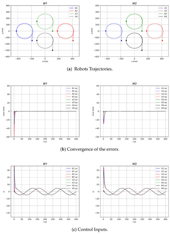
Figure 10.
Numerical simulation with the 4 Robot diamond-shaped formation topology.
The adjacent subsets for the real robots are defined as , , , , , , , , as shown in Figure 5. The target final pattern configuration for the robots is a diamond-shaped formation, as if all four real robots were operating within the same workspace. To achieve this arrangement, the corresponding relative vectors are defined by , , , , with , , and by construction , , , and .
Figure 10 shows the trajectories of the real and virtual robots using the control law (4)–(5)–(6) with unitary values of gains , , and and the desired trajectory of the leader robot given by . It can be observed that the robots converge to the intended formation, as evidenced by the error convergence presented in Figure 10b. Additionally, Figure 10c illustrates the control inputs.
In the third formation, as shown in Figure 5, several simulations were performed by varying the parameters , , and to assess the stability and convergence rate of the control strategy. Simulations were conducted using k values of , 1, and 10, as well as their different combinations, while ensuring that remained greater than or equal to both and . For each simulation, the and norms were calculated by summing the absolute errors and squared errors, respectively, taking into account errors from both workspaces and from both real and virtual robots. The results are depicted in the graphs in Figure 11 and summarized in Table 3.
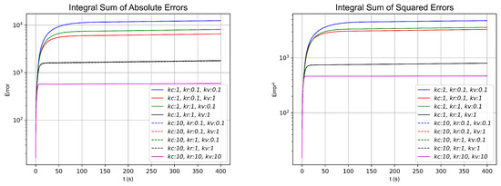
Figure 11.
and norms with different k values in the diamond-shaped Robot simulation.
Table 3.
and norms for different k values in the 4 Robot diamond-shaped simulation.
As shown in the numerical simulations and the results presented in Table 1, Table 2 and Table 3 for the different topologies and formations, as well as in the simulations conducted with various k gain values, higher k gains yield a faster and more pronounced convergence. This is evident in the figures illustrating the and norms for the three configurations: two robots arranged in a horizontal line (Figure 7), four robots arranged in a horizontal line (Figure 9), and four robots in a diamond-shaped formation (Figure 11). The most influential gains in the control model are and , since identical values for these parameters result in similar convergence rates and comparable and norm values even when varies. For example, when examining the black curve (a continuous or dashed line) corresponding to set to 1 or 10 with and both fixed to , both simulations exhibit similar convergence speeds and behavior, despite the variation in also having a similar value to and norm values.
4.2. With Communication Delays
Numerical simulations were performed using the previously described control strategy with fixed gain values (, , ). The same three topologies and workspace configurations presented earlier were employed, with the added feature of introducing a controlled constant delay in the position information of the virtual robots, which receive data directly from their corresponding real robot in the other workspace. This delay, denoted as , was tested at various values ( and 10 s) to evaluate the convergence speed and stability of the control strategy in the presence of delays. The maximum delay value simulated for these tests was selected based on the experimental work discussed in Section 5.2 and Section 5.3. This study focuses on using the MQTT communication platform, which exhibits an average delay of s and can reach maximum delays of up to 2 s. Also, a delay of 0.1 s in the computer vision system was measured for robot position detection. Consequently, intermediate delay values within this range were evaluated in various numerical simulation tests in the current section.
Figure 12 shows an example of a numerical simulation based on the workspace and topology formation shown in Figure 3, now developed in this example with a delay s with respect to the data of the virtual robots. Note that an increase in the error values and a delay in the relative position of virtual and real robots was generated compared to the simulation shown in Figure 6.

Figure 12.
Numerical simulation for 2-robot horizontal line shape formation with delays.
In the first formation, as shown in Figure 3, several simulations were performed by varying the delay to assess the stability and convergence rate of the control strategy. For each simulation, the and norms were calculated by summing the absolute errors and squared errors, respectively, taking into account errors from both workspaces and from both real and virtual robots. The results are depicted in the graphs in Figure 13 and summarized in Table 4.
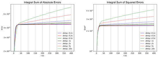
Figure 13.
and norms with different delays for the simulation of 2-robot horizontal line shape formation.
Table 4.
and norms for different values for the simulation of 2-robot horizontal line shape formation.
In Figure 14, the same numerical simulation is also developed with a delay s with respect to the data of the virtual robots, now based on the workspace and topology formation as shown in Figure 4. An increase in error values can be observed, along with a delay in the relative positioning between virtual and real robots, compared to the simulation presented in Figure 8.
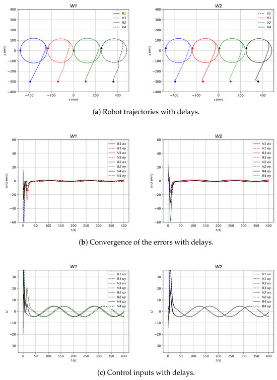
Figure 14.
Numerical simulation of 4-robot horizontal line shape formation with delays.
In the second formation, as shown in Figure 4, the same simulations were performed, varying the delay to assess the stability and convergence rate of the control strategy. For each simulation, the and norms were calculated, and the results are depicted in the graphs in Figure 15 and summarized in Table 5.
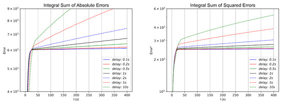
Figure 15.
and norms with different delays in simulation of 4-robot horizontal line shape formation.
Table 5.
and norms for different values in simulation of 4-robot horizontal line shape formation.
Figure 16 is an example of the same numerical simulation developed with a delay s with respect to the data of the virtual robots, now based on the workspace and topology formation shown in Figure 5. An increase in error values can be observed, along with a delay in the relative positioning between virtual and real robots, compared to the simulation presented in Figure 10.
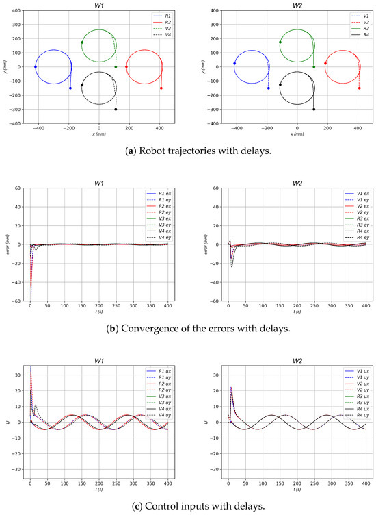
Figure 16.
Numerical simulation with the 4 Robot diamond-shaped formation topology with delays.
In the third formation, as shown in Figure 5, the same simulations were performed, varying the delay to assess the stability and convergence rate of the control strategy. For each simulation, the and norms were calculated; the results are depicted in the graphs in Figure 17 and summarized in Table 6.
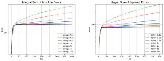
Figure 17.
and norms different delay in the 4 Robot diamond-shaped simulation.
Table 6.
and norms for different values in the 4 Robot diamond-shaped simulation.
As shown in the numerical simulations and the results presented in Table 4, Table 5 and Table 6 for the different topologies and formations, as well as in the simulations conducted with various delay values at , a lower delay value, ideally approaching zero, yields a faster and more pronounced convergence. This is evident in the figures illustrating the norms and for the three configurations in Figure 13, Figure 15, and Figure 17. All tests converge regardless of the selected delay value. In particular, as mentioned earlier, our primary interest lies in delays close to s, the average delay of MQTT communications, and sporadic delays of up to 2 s. In all tests conducted, even with delay values exceeding those expected in future experiments, the numerical simulations of the three formations under this control strategy successfully converged. Although higher delays result in a slower convergence rate and an increase in accumulated error, all experiments maintained stable results, exhibiting only minor oscillations attributable to the data delay.
5. Experimental Work
The control implementation for all cyber–physical experiments is presented in Figure 18. The n robots are placed in two different workspaces. Every workspace has a web camera (Model , Logitech, Lausanne, Switzerland) with a resolution of pixels, installed at a height of 400 mm, that generates a viewing area of around 750 mm × 400 mm. Every camera is connected to a PC computer (Model Core , Intel Corp., Santa Clara, CA, USA). The PC reads the Aruco tags (OpenCV-contrib module, OpenCV.org, Palo Alto, CA, USA) at a sample rate of s, detecting the of the robots and calculating the position and orientation of every robot using a visual processing library (OpenCV 4.8.0, OpenCV.org, Palo Alto, CA, USA). The positions and orientations are processed by the computer in the workspace for the real robots, and this same information is sent to the internet through an IoT protocol (MQTT v3.1.1 and 1.6.9, Eclipse Foundation, Ottawa, ON, Canada). using different brokers. The communication is bidirectional, and the two workspaces are connected via the internet. The control law was programmed in each PC using Python (Version , Python Software Foundation, Wilmington, DE, USA), sending the control inputs to every robot using Bluetooth wireless communication. Note that the control setup is low-cost and scalable. Also, the experimental setup is modular using commercial components, allowing its expansion to more robots and workspaces. Figure 19 is an example of the control implementation using the experimental platform of the topology and the formation structure of the four-robot diamond shape based on the topology shown in Figure 5.
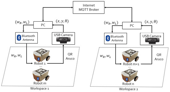
Figure 18.
Workspace diagram for the cyber–physical experiments.
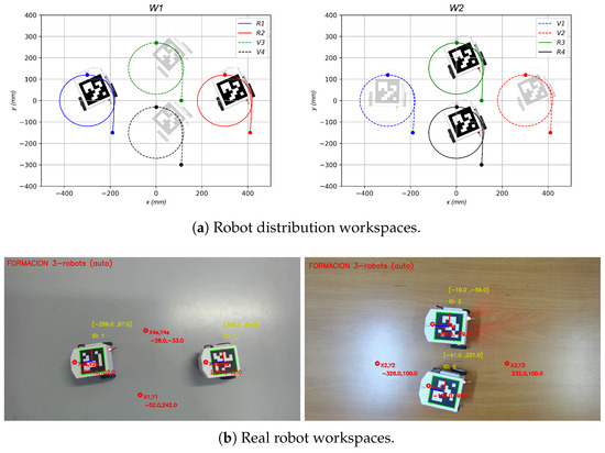
Figure 19.
Control implementation workspace example.
5.1. Unicycle-Type Robots
The control approach was tested in a low-cost experimental robotic platform composed of the four mobile robots shown in Figure 20. Each unicycle-type robot was integrated with two DC motors (Micro metal gear motors HP 6v 1000:1, Pololu Corporation, Las Vegas, NV, USA) with plastic wheels, controlled by a microcontroller (ATmega32U4-based microcontroller, Arduino SA, Somerville, MA, USA). with Bluetooth wireless communication to a PC. The robot case was made with a 3D printer with an Aruco tag on top. The unicycle robots measure 100 mm × 100 mm; this size was selected during development to provide a versatile, easily maneuverable platform that is well suited for both academic and research environments.
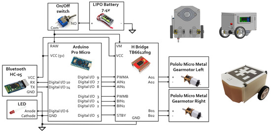
Figure 20.
Diagram of the electronics system for the robots’ experimental setup.
A detailed breakdown of the main hardware components and their estimated prices is given in Table 7. The total cost per unit is estimated to be in the range of USD 40 to 70, which is significantly lower than similar platforms described in the literature (typically USD 80 to 150).
Table 7.
Unicycle type robot components and costs.
This cost-effective design reduces the experimentation cost for multiple robots or multiple workspaces and also facilitates easy replication and scalability in academic and research settings.
The kinematic model of the unicycle-type robots shown in Figure 20 is given, according to Figure 21, by
with , where is the 2D coordinate of the robot and is its orientation angle with respect to the horizontal axis. The and are the longitudinal and rotational control inputs with respect to the middle point of the axis wheels. These two body-level velocities can be converted to the velocities of the wheels through
where and are the angular velocities of the right and left wheels, respectively, r is the radius of the wheels, and L is the distance between the wheels.
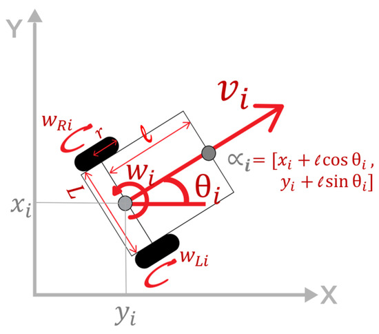
Figure 21.
Kinematic model of a unicycle-type robot.
The frontal point is chosen as control output, shown in Figure 21 with
where . Its dynamics are given by
where . Since , it is possible to linearize the dynamics of using the control
with as an auxiliary control. Note that in the closed-loop control (26) and (27), the dynamics is reduced to and the nonlinearities are eliminated, resulting in the single integrator given by (3). Therefore, the control approach can be extended to the unicycle-type robots using the control law (27), where is defined by the Equations (4)–(6) but dependent on the coordinates of the robots. For the experimental work case developed in Section 5.4, the parameters of the robots constructed for the experimental platform in this study are mm, mm, and mm. Here, r is defined as the radius of the robot’s wheel, ℓ is the distance to an auxiliary frontal point, and L is the distance between the centers of the two wheels. These values are determined by the size of the robot and the commercial components used. Additionally, due to the selected motor type Pololu© 6V with a 1000:1 gear ratio and a maximum speed of 33 RPM and given the wheel radius of mm, the robot and control programming impose a maximum wheel angular velocity of rad/s and a minimum value of rad/s, which is approximately of the motors’ maximum speed.
5.2. MQTT Broker
For the MQTT IoT connection, Python and the paho.mqtt library were used to establish communication between the computer and the MQTT server (broker). An MQTT broker is a message intermediary that facilitates communication between devices and applications via the MQTT protocol; it manages the publication and subscription of messages and topics. In this experiment, two different brokers were employed: a popular commercial broker, test.mosquitto.org, and a custom-developed broker hosted on Google Cloud.
The broker test.mosquitto.org, is a free commercial broker accessible on port 1883 that does not require encryption or authentication, making it commonly used for MQTT development and testing. Also, a custom MQTT broker was developed using the Google Cloud platform. A virtual machine instance of type “e2-medium” with two virtual CPUs, 4 GB of RAM, and Ubuntu as the operating system was created. Port 1883 was enabled, and the mosquitto and mosquitto-client packages (versions 1.6.9 and 3.1.1) were installed. Once configured, the public IP of the server was obtained for directing messages to the appropriate IP and port.
For both brokers, latency and communication tests were performed by sending 4000 data packets at a sampling rate of s, measuring the time required for data transmission between computers. In Figure 22, the latency times for the test.mosquitto.org broker are shown, with an average of s and a standard deviation of s, indicating a highly stable broker with occasional maximum latencies of s. In contrast, the Google Cloud broker exhibits an average latency of s and a standard deviation of , making it less stable than the commercial broker, with sporadic latencies reaching 2 s.
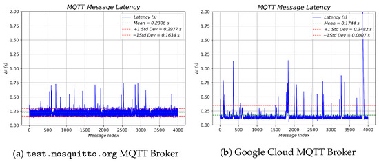
Figure 22.
MQTT brokers latency, mean, and standard deviation.
5.3. Position Detection with Aruco QR Code and Computer Vision
For robot position detection, Python was utilized along with the OpenCV library to detect ArUco-type QR codes. The detection algorithm provides the x and y coordinates, as well as the orientation angle for each robot. Latency tests were carried out to evaluate the processing speed and potential delays when detecting or 4 QR codes, as shown in Table 8, with the latency remaining constant at approximately s and a minimal standard deviation of s. In Figure 23b, the results from a test involving 1000 frames capturing four QR codes on four robots confirm that the latency is maintained throughout the experiment.
Table 8.
Mean and standard deviation of the Aruco QR code detection latency.
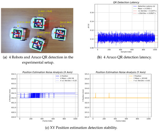
Figure 23.
QR computer vision latency and stability.
Additionally, the vision system employs a Logitech C920© camera with a resolution of 1280 × 720 pixels. The camera is positioned 400 mm above the robot formation area, and its field of view covers an area of 750 mm by 400 mm, resulting in a per-pixel area of mm2. A stability test was performed by measuring the x and y positions of a fixed QR code without moving either the QR code or the camera, thereby assessing the system’s stability. As depicted in Figure 23c, based on 1000 frames captured of a stationary QR code, the measurements yielded a standard deviation of mm, indicating a resolution of less than 1 mm.
5.4. Experimental Results
Using the experimental platform, several experiments were conducted with the formation configurations presented in the simulation Section 4 (Figure 3, Figure 4 and Figure 5). Based on the numerical simulations, a unit gain (, and ) was selected for the physical experiments. Each experiment was carried out with a different sampling time (), which determines both the calculation frequency and the rate at which data are transmitted to the MQTT broker. Sampling times of and s were tested. It is important to note that several of these sampling rates exceed the previously studied data transmission rate of the MQTT system (an average of s) and the camera sampling rate ( s). This introduces expected errors and delays in the data, as discussed in the numerical simulation section regarding the robustness of the control model. In addition to testing different parameters, the experiments were carried out using two distinct MQTT brokers: a popular commercial broker, test.mosquitto.org, and a custom-developed broker hosted in Google Cloud. The errors of all experiments were quantified using comparative tables based on the integral of the norm (sum of absolute errors) and the norm (sum of squared errors).
Figure 24 shows the experimental results of the simulation with . The desired trajectory of the leader robot is given by in millimeters, and the MQTT broker selected for this specific experiment was the comercial MQTT broker test.mosquitto.org. The robots converge to the desired formation pattern, which is observed by the robots’ trajectories in Figure 24a and the error convergence shown in Figure 24b. Note that the errors of the real robots are smaller than the errors of the virtual robots in the experimental data. The control inputs are depicted in Figure 24c, and note that the control input is saturated at a maximum value and a minimum value of . Note that the control performance is affected by the resolution of the camera, the sample time, and the non-modeled dynamics presented by the floor friction and other real effects.
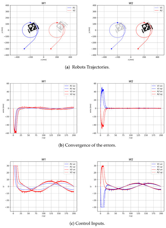
Figure 24.
Experimental results for a 2-robot horizontal line shape formation.
Figure 25 illustrates the longitudinal velocity values V relative to the midpoint between the wheel axes; see Figure 25a. Furthermore, Figure 25b presents the angular velocities, and , corresponding to the right and left wheels of each robot, respectively. Note that the angular wheel velocities are saturated at a maximum value of rad/s and a minimum value of , due to the maximum speed that the physical motors on the experimental platform can achieve.
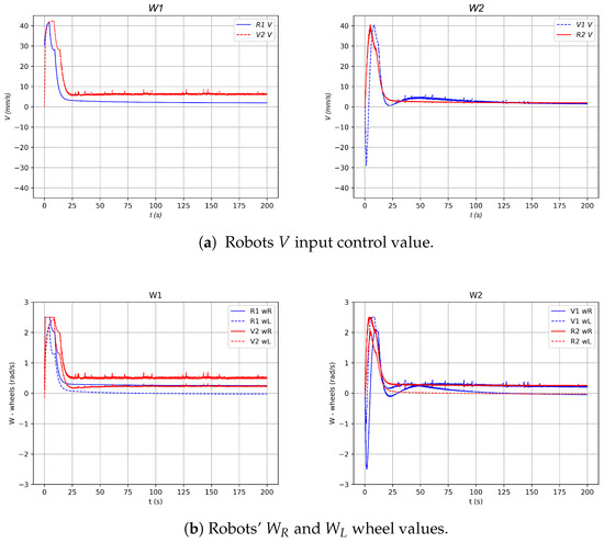
Figure 25.
V, , and values in the experiment of 2-robot horizontal line shape formation.
In this first formation topology, as shown in Figure 3, several experiments were performed by varying the sample rate to assess the stability and convergence rate of the control strategy. The simulations were carried out using different values of , and , and all the different dt values were evaluated with different MQTT brokers: test.mosquitto.org and a custom-developed broker hosted on Google Cloud. For each simulation, the and norms were calculated by summing the absolute errors and squared errors, respectively, taking into account errors from both workspaces and from both real and virtual robots. The results of the different broker test are shown in the graphs in Figure 26 and summarized in Table 9. Additionally, graphs were generated that depict the instantaneous sum of squared errors (computed by aggregating the errors of each real or virtual robot across both workspaces) to compare which sampling times and MQTT broker configurations offer the greatest stability and the fastest convergence, despite system delays and other challenges inherent in physical robot experiments. These results are illustrated in Figure 27.
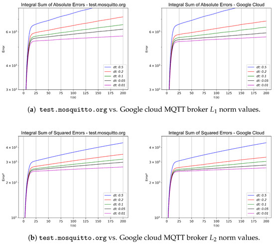
Figure 26.
and norms in the experiment of 2-robot horizontal line shape formation.
Table 9.
and norms in the experiment of 2-robot horizontal line shape formation. (a) test.mosquitto.org MQTT Broker; (b) Google Cloud MQTT Broker.
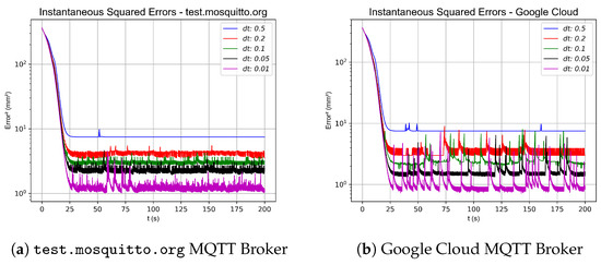
Figure 27.
Instantaneous squared error in the experiment of 2-robot horizontal line shape formation.
Figure 28 shows the second experiment with a ; the desired trajectory of the leader robot is given by in millimeters and the same MQTT broker, namely test.mosquitto.org. The robots converge to the desired formation pattern, which is observed by the robots’ trajectories in Figure 28a and the error convergence shown in Figure 28b. Note that the errors of the real robots are smaller than the errors of the virtual robots in the experimental data. The control inputs are depicted in Figure 28c, and note that the control input is saturated at a maximum value and a minimum value of . Note that the control performance is affected by the resolution of the camera, the sample time, and the non-modeled dynamics presented by the floor friction and other real effects.
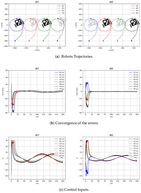
Figure 28.
Experimental results of 4-robot horizontal line shape formation.
Figure 29 illustrates the longitudinal velocity values V relative to the midpoint between the wheel axes; see Figure 29a. Furthermore, Figure 29b presents the angular velocities, and , corresponding to the right and left wheels of each robot, respectively. Note that the angular wheel velocities are saturated at a maximum value of rad/s and a minimum value of due to the maximum speed that the physical motors on the experimental platform can achieve.
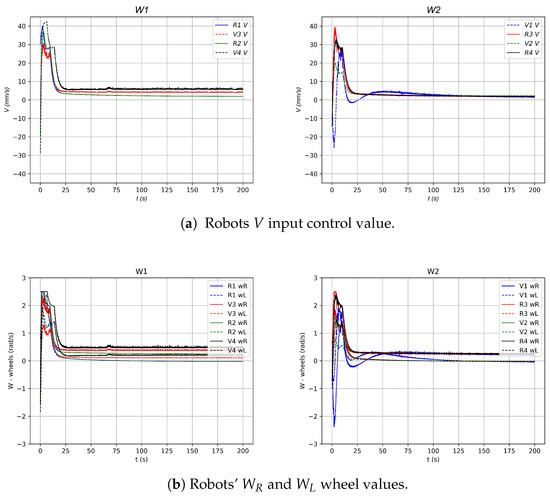
Figure 29.
V, , and values in the experiment of 4-robot horizontal line shape formation.
In the second formation topology, as shown in Figure 4, several experiments were performed by varying the sample rate to assess the stability and convergence rate of the control strategy. In this formation, new experiments were also carried out using different values and with different MQTT brokers. For each simulation, the and norms were calculated by summing the absolute errors and squared errors, respectively, taking into account errors from both workspaces and from both real and virtual robots. The results of the different broker test are shown in the graphs in Figure 30 and summarized in Table 10. Additionally, graphs were generated that depict the instantaneous sum of squared errors (computed by aggregating the errors of each real or virtual robot across both workspaces) to compare which sampling times and MQTT broker configurations offer the greatest stability and the fastest convergence, despite system delays and other challenges inherent in physical robot experiments. These results are illustrated in Figure 31.
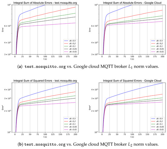
Figure 30.
and norms in the experiment of 4-robot horizontal line shape formation.
Table 10.
and norms in the experiment of 4-robot horizontal line shape formation. (a) test.mosquitto.org MQTT broker. (b) Google Cloud MQTT broker.
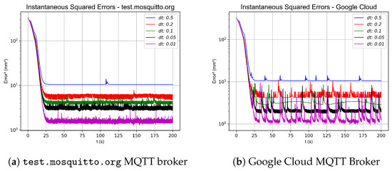
Figure 31.
Instantaneous Squared error in the experiment of 4-robot horizontal line shape formation.
Figure 24 shows the experimental results with a ; the desired trajectory of the leader robot is given by in millimeters and the MQTT broker test.mosquitto.org. The robots converge to the desired formation pattern. The robots’ trajectories are observed in Figure 32a, and error convergence is shown in Figure 32b. Note that the errors of the real robots are smaller than the errors of the virtual robots in the experimental data. The control inputs are depicted in Figure 32c, and note that the control input is saturated at a maximum value and a minimum value of . Note that the control performance is affected by the resolution of the camera, the sample time, and the non-modeled dynamics effects.
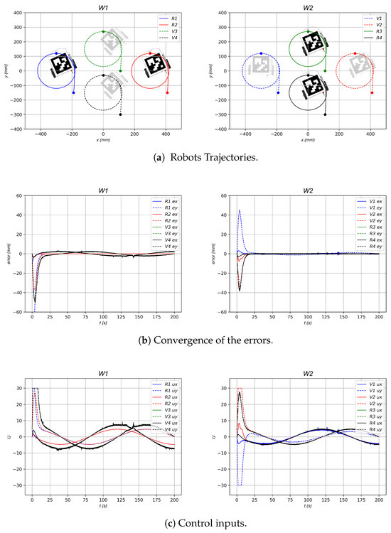
Figure 32.
Experimental work with the 4 Robot diamond-shaped workspace and formation topology.
Figure 33 illustrates the longitudinal velocity values V relative to the midpoint between the wheel axes (see Figure 33a). Furthermore, Figure 33b presents the angular velocities, and , corresponding to the right and left wheels of each robot. Both are saturated at a maximum value of and a minimum value of , due to the maximum speed that the physical motors of the real robots can achieve.
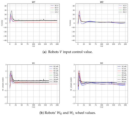
Figure 33.
V, and values in the 4 Robot diamond-shaped formation topology experiment.
In the third formation topology, as shown in Figure 5, several experiments were performed by varying the sample rate to assess the stability and convergence rate of the control strategy. In this formation, new experiments were also carried out using different values and with different MQTT brokers. For each experiment, the and norms were calculated by summing the absolute errors and squared errors, respectively, taking into account errors from both workspaces and from both real and virtual robots. For each simulation, the and norms were calculated by summing the absolute errors and squared errors, respectively, taking into account errors from both workspaces and from both real and virtual robots.The results of the different broker test are shown in the graphs in Figure 34 and summarized in Table 11. Furthermore, graphs were generated that depict the instantaneous sum of squared errors (computed by aggregating the errors of each real or virtual robot across both workspaces) to compare which sampling times and MQTT broker configurations offer the greatest stability and the fastest convergence, despite system delays and other challenges inherent in physical robot experiments. These results are illustrated in Figure 35.
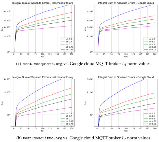
Figure 34.
and norms in the 4 diamond-shaped Robot experiment.
Table 11.
and norms with in the 4 diamond-shaped Robot experiment. (a) test.mosquitto.org MQTT broker. (b) Google Cloud MQTT broker.
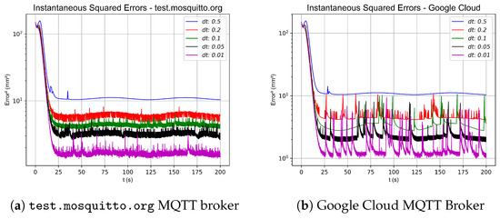
Figure 35.
Instantaneous squared error in the 4 diamond-shape Robot experiment.
As shown in the numerical simulations and the results presented in Table 9, Table 10 and Table 11 for the different topologies and formations, as well as in the simulations conducted with various sampling times , and also using different MQTT brokers, a lower sampling time , ideally approaching zero, even with more communication errors, yields a faster and more pronounced convergence. This is evident in the figures illustrating the norms and for the three configurations in Figure 26, Figure 30, and Figure 34.
Furthermore, an analysis of the and norm tables from the three experiments shows no significant differences between the commercial broker test.mosquitto.org and the Google Cloud broker. In particular, in all experiments, the Google Cloud broker yielded slightly lower and norm values, indicating reduced errors with this MQTT service. This result is directly related to the latency and transmission speeds measured in Section 5.2, where test.mosquitto.org exhibited an average latency of s, while the Google Cloud broker showed a latency of s, as illustrated in Figure 22.
It is also important to mention that although the Google Cloud broker has a higher standard deviation in transmission time and occasionally experiences significant delays of and 2 s, the control strategy remains robust enough to benefit from its lower average latency and faster sampling times. Figure 27, Figure 31, and Figure 35 display the instantaneous sum of squared errors for both brokers in the three different topologies; for test.mosquitto.org, the error is relatively constant with occasional peaks due to communication delays and platform limitations, whereas the Google Cloud broker exhibits a general lower error value but is less consistent and more erratic. However, when integrating the absolute and squared errors to compute the and norms, the values are lower for the Google Cloud broker compared to the commercial alternative. Regarding convergence speed, the control model and the numerical simulation results, illustrated in Table 1, Table 2 and Table 3 for the different topologies and formations, as well as the simulations conducted with various controller gains values (, , ), show that higher controller gains yield a faster and more pronounced convergence. Thus, increasing the gain results in a more rapid convergence of the system. Another critical factor is the latency introduced by the MQTT broker communications and the delays associated with the computer vision system. As shown in the numerical simulations and the results presented in Table 4, Table 5 and Table 6 for the different topologies and formations, as well as the simulations conducted with various delay values at , a lower delay, ideally approaching zero, leads to a faster and more pronounced convergence. Finally, additional factors that affect the convergence speed in the experiments include the maximum velocity of the robot. As explained in Section 5.1, given the maximum speed of 33 RPM and a radius of the wheels of , the control system limits the maximum angular velocity of the wheels to . Moreover, the initial positions of the robots play a significant role; starting from positions that are distant from the desired trajectory or formation will increase the convergence time due to the imposed speed limitations.
Another important detail to consider is that the errors observed in the real robots are smaller than those measured in the virtual robots in the experimental data. This difference is attributed to the inherent communication delays affecting the virtual robots whose positional data include the latency of data transmission, whereas the real robots only experienced the delay associated with the computer vision-based positioning system. Moreover, due to the formation and relative vectors, the virtual robots in workspace 1 incurred a double communication delay: the first delay originated from the virtual robots in workspace 2, and the second arose from the additional latency when transmitting the relative position data of the real robots in workspace 2 back to workspace 1. This results in two accumulated delays in the overall experimental cycle.
6. Conclusions
This paper presents a comprehensive model of cyber–physical formations, offering clear insights into their design, control, and experimentation. The approach is given by mobile robots represented as a single integrator moving in a plane. These robots move in two different workspaces, sharing their postures through the internet. The control law is designed to ensure the convergence of the robots to a formation pattern as if they moved in a single workspace. The control law is designed for a general case of n robots.
The control strategy uses virtual agents that converge to the physical robots moving in the opposite workspace. Two cases were studied: first, a formation convergence without communication delays in measuring the robot’s postures, and second, the effect of communication delays when the posture of robots is transmitted over the internet. The latter case is particularly relevant for real-world applications where workspaces are distant from each other and information transmission can be significantly delayed. Other practical drawbacks can generate these delays as part of the cyber–physical setups different from formations made in a single workspace. The convergence of the control law is analyzed and validated through numerical simulations.
In addition, as a proof of concept, the control law is extended to the case of unicycle-type robots. A cost-effective experimental platform is then designed and assembled using commercial electronics and common 3D-printer-based manufacturing techniques. The robots are placed in two different physical workspaces with internet communication using Bluetooth wireless communication and the MQTT protocol. This setup allows for the experimental testing of two distinct control scenarios: one involving delays and the other without delays. The experiment aims to calculate the inherent packet delivery time of the MQTT server. The experiments demonstrate the performance of the control law and its applicability to practical problems.
It should be noted that the approach of virtual agents can be extended to the case of agents moving in 3D in cyber–physical scenarios including more than two workspaces. The control scheme can be applied to different practical multi-robot tasks, where the coordinated motion of robots in different workspaces or internet networks offers some advantages. For instance, it can emulate mirror effects of robots moving outdoors with a physical remote telepresence in a control station room. Additionally, it can be utilized in formations of robots that are not necessarily in different spaces but connected via separate routers and internet networks, as is typical in factory plants and similar environments. It is also noted that the virtual and real agents can be strategically switched, e.g., when a real robot fails, and it might be convenient to switch to a virtual robot in order to maintain the formation pattern. A significant contribution of this paper is the demonstration of a minimal setup with a single model of robots in a cyber–physical system as the foundation for future extensions and applications.
In future work, improvements will focus on the dynamical modeling of robots, as well as the integration of heterogeneous robot formations, including unicycle-type, omnidirectional, car-like, and other common vehicle models. While the primary focus of this work is on achieving convergence in multi-robot formations, the integration of these diverse models is crucial for enhancing the versatility and efficacy of robotic systems. However, collision avoidance is a critical aspect for ensuring safe operations, especially during transient phases. Therefore, some robust collision-avoidance mechanisms will be investigated in the multi-robot coordination framework. Also, other drawbacks related to internet communication can be addressed, such as intermittency effects, non-fixed delay times, and other expected effects that commonly occur in cyber–physical environments.
Author Contributions
Conceptualization , E.G.H.-M. and J.-J.F.-G.; methodology E.D.F.-V. and E.G.H.-M.; software, H.G.-N. and A.M.-J.; validation, H.G.-N.; formal analysis, E.D.F.-V.; investigation, M.R.-N.; resources, E.G.H.-M.; writing—original draft preparation, G.F.-A. and H.G.-N.; writing—review and editing, A.M.-J. and J.-J.F.-G.; visualization, E.D.F.-V. and H.G.-N.; project administration G.F.-A.; funding acquisition, E.G.H.-M. All authors have read and agreed to the published version of the manuscript.
Funding
This work was supported by project DINVP-051 from the Institute of Applied Research and Technology (INIAT) at Universidad Iberoamericana Ciudad de México, México and by project 5152-25805 from the Institute of Design and Innovation Technology (IDIT) at Universidad Iberoamericana Puebla, México.
Data Availability Statement
The data that support the findings of this study are available from the author, Huber Giron-Nieto, upon reasonable request to huber.giron2@iberopuebla.mx.
Conflicts of Interest
The authors declare no conflicts of interest.
References
- Canudas de Wit, C.; Siciliano, B.; Bastin, G. (Eds.) Theory of Robot Control; Springer: London, UK, 1996. [Google Scholar]
- Valentim, T.; Cunha, R.; Oliveira, P.; Cabecinhas, D.; Silvestre, C. Multi-vehicle Cooperative Control for Load Transportation. IFAC-PapersOnLine 2019, 52, 358–363. [Google Scholar] [CrossRef]
- Matsuo, R.; Yasuda, S.; Kumagai, T.; Sato, N.; Yoshida, H.; Yairi, T. Residual reinforcement learning for logistics cart transportation. Adv. Robot. 2022, 36, 404–421. [Google Scholar] [CrossRef]
- Lopes, S.L.; Ferreira, A.I.; Prada, R.; Schwarzer, R. Social robots as health promoting agents: An application of the health action process approach to human-robot interaction at the workplace. Int. J. Hum.-Comput. Stud. 2023, 180, 103124. [Google Scholar] [CrossRef]
- Gasparino, M.V.; Higuti, V.A.; Sivakumar, A.N.; Velasquez, A.E.; Becker, M.; Chowdhary, G. CropNav: A Framework for Autonomous Navigation in Real Farms. In Proceedings of the 2023 IEEE International Conference on Robotics and Automation (ICRA), London, UK, 29 May–2 June 2023; pp. 11824–11830. [Google Scholar] [CrossRef]
- Vichare, S.; Katare, S.; Pawar, A. Wireless Military Defense Robot. Int. Res. J. Eng. Technol. (IRJET) 2020, 7, 88–95. [Google Scholar]
- Benazir Begam, R.; Yogalakshmi, V.; Sanjai Nagaraaja, M.; Sanjay Kumar, A.; Santhosh Priyan, A. IoT based Multipurpose Agricultural Robot. In Proceedings of the 2024 3rd International Conference on Applied Artificial Intelligence and Computing (ICAAIC), Salem, India, 5–7 June 2024; pp. 1755–1761. [Google Scholar] [CrossRef]
- Do, K.D. Formation tracking control of unicycle-type mobile robots. In Proceedings of the 2007 IEEE International Conference on Robotics and Automation, Roma, Italy, 10–14 April 2007; pp. 2391–2396. [Google Scholar]
- Fei, Y.; Shi, P.; Lim, C.P.; Yuan, X. Finite-time observer-based formation tracking with application to omnidirectional robots. IEEE Trans. Ind. Electron. 2022, 70, 10598–10606. [Google Scholar] [CrossRef]
- Hernandez-Martinez, E.G.; Foyo-Valdes, S.A.; Puga-Velazquez, E.S.; Meda-Campaña, J.A. Hybrid architecture for coordination of AGVs in FMS. Int. J. Adv. Robot. Syst. 2014, 11, 41. [Google Scholar] [CrossRef]
- Farrugia, J.L.; Fabri, S.G. Swarm Robotics for Object Transportation. In Proceedings of the 2018 UKACC 12th International Conference on Control (CONTROL), Sheffield, UK, 5–7 September 2018; pp. 353–358. [Google Scholar]
- Ferreira-Vazquez, E.D.; Hernández-Martínez, E.G.; Flores-Godoy, J.J.; Fernandez-Anaya, G.; Paniagua-Contro, P. Distance-based formation control using angular information between robots. J. Intell. Robot. Syst. 2016, 83, 543–560. [Google Scholar] [CrossRef]
- Oh, K.K.; Park, M.C.; Ahn, H.S. A survey of multi-agent formation control. Automatica 2015, 53, 424–440. [Google Scholar] [CrossRef]
- Lopez-Gonzalez, A.; Ferreira, E.; Hernández-Martínez, E.G.; Flores-Godoy, J.J.; Fernandez-Anaya, G.; Paniagua-Contro, P. Multi-robot formation control using distance and orientation. Adv. Robot. 2016, 30, 901–913. [Google Scholar] [CrossRef]
- Keung, K.L.; Lee, C.K.M.; Ji, P.; Ng, K.K.H. Cloud-Based Cyber-Physical Robotic Mobile Fulfillment Systems: A Case Study of Collision Avoidance. IEEE Access 2020, 8, 89318–89336. [Google Scholar] [CrossRef]
- Dang, T.V.; Bui, N.T. Obstacle avoidance strategy for mobile robot based on monocular camera. Electronics 2023, 12, 1932. [Google Scholar] [CrossRef]
- Escobar, L.; Moyano, C.; Aguirre, G.; Guerra, G.; Allauca, L.; Loza, D. Multi-Robot platform with features of Cyber–physical systems for education applications. In Proceedings of the 2020 IEEE ANDESCON, Quito, Ecuador, 13–16 October 2020; pp. 1–6. [Google Scholar]
- Samie, F.; Bauer, L.; Henkel, J. IoT technologies for embedded computing: A survey. In Proceedings of the 2016 International Conference on Hardware/Software Codesign and System Synthesis (CODES+ISSS), Pittsburgh, PA, USA, 2–7 October 2016; pp. 1–10. [Google Scholar]
- Nemade, B.; Phadnis, N.; Desai, A.; Mungekar, K.K. Enhancing connectivity and intelligence through embedded Internet of Things devices. ICTACT J. Microelectron. 2024, 9, 1670–1674. [Google Scholar] [CrossRef]
- Deng, Y.; Léchappé, V.; Moulay, E.; Chen, Z.; Liang, B.; Plestan, F.; Han, Q.L. Predictor-based control of time-delay systems: A survey. Int. J. Syst. Sci. 2022, 53, 2496–2534. [Google Scholar] [CrossRef]
- Kharitonov, V. Time-Delay Systems: Lyapunov Functionals and Matrices; Springer Science & Business Media: Boston, MA, USA, 2012. [Google Scholar]
- Mondie, S.; Kharitonov, V.L. Exponential estimates for retarded time-delay systems: An LMI approach. IEEE Trans. Autom. Control. 2005, 50, 268–273. [Google Scholar] [CrossRef]
- Trinh, H. Exponential stability of time-delay systems via new weighted integral inequalities. Appl. Math. Comput. 2016, 275, 335–344. [Google Scholar]
- Notomista, G.; Cai, X.; Egerstedt, M. Passivity-Based Decentralized Control of Multi-Robot Systems With Delays Using Control Barrier Functions. arXiv 2019, arXiv:1904.04801. [Google Scholar]
- Karafyllis, I.; Malisoff, M.; Mazenc, F.; Pierdomenico Pepe, E. Recent Advances in Nonlinear Delay Control Systems. In Advances in Delays and Dynamics; Springer: Cham, Switzerland, 2016. [Google Scholar]
- Lian, Y.; Xie, W.; Yang, Q.; Zhang, L.; Lin, D.; Zhou, Y. A Novel Multi-Warehouse Mobile Robot Hierarchical Scheduling Strategy Based on Industrial Cyber-Physical System. In Proceedings of the 2021 4th IEEE International Conference on Industrial Cyber-Physical Systems (ICPS), Virtual Conference, 10–12 May 2021; pp. 263–269. [Google Scholar]
- Pikner, H.; Sell, R.; Karjust, K.; Malayjerdi, E.; Velsker, T. Cyber–physical Control System for Autonomous Logistic Robot. In Proceedings of the 2021 IEEE 19th International Power Electronics and Motion Control Conference (PEMC), Gliwice, Poland, 25–29 April 2021; pp. 699–704. [Google Scholar]
- Kruglova, T.; Schmelev, I.; Sushkov, I.; Filatov, R. Cyber–physical System of the Mobile Robot’s Optimal Trajectory Planning with taking into account Electric Motors Deterioration. In Proceedings of the 2019 International Multi-Conference on Industrial Engineering and Modern Technologies (FarEastCon), Vladivostok, Russia, 1–4 October 2019; pp. 1–5. [Google Scholar]
- Guan, J.; Zhou, W.; Kang, S.; Sun, Y.; Liu, Z. Robot Formation Control Based on Internet of Things Technology Platform. IEEE Access 2020, 8, 96767–96776. [Google Scholar] [CrossRef]
- de Morais, H.R.F.; de Almeida, J.P.L.S.; de Arruda, L.V.R. Running Cooperative Tasks in a Multi-Robot System with Cyber-Physical Features. In Proceedings of the 2022 Latin American Robotics Symposium (LARS), 2022 Brazilian Symposium on Robotics (SBR), and 2022 Workshop on Robotics in Education (WRE), Sao Paulo, Brazil, 18–21 October 2022; pp. 217–222. [Google Scholar]
- Li, W.; Wu, J.; Long, C. Formation Control for Unmanned Surface Vehicles Based on Integrative APF and MPC. In Proceedings of the 2022 IEEE International Conference on Robotics and Biomimetics (ROBIO), Xishuangbanna, China, 5–9 December 2022; pp. 201–206. [Google Scholar]
- Kivrak, H.; Karakusak, M.Z.; Watson, S.; Lennox, B. Cyber–physical system architecture of autonomous robot ecosystem for industrial asset monitoring. Comput. Commun. 2024, 218, 72–84. [Google Scholar] [CrossRef]
- Xie, J.; Liu, S.; Wang, X. Framework for a closed-loop cooperative human Cyber-Physical System for the mining industry driven by VR and AR: MHCPS. Comput. Ind. Eng. 2022, 168, 108050. [Google Scholar] [CrossRef]
- Kim, K.J.; Suh, I.H.; Kim, S.H.; Oh, S.R. A novel real-time control architecture for internet-based thin-client robot; simulacrum-based approach. In Proceedings of the 2008 IEEE International Conference on Robotics and Automation, Pasadena, CA, USA, 19–23 May 2008; pp. 4080–4085. [Google Scholar]
- Nanu, L.; Colangelo, L.; Novara, C.; Montenegro, C.P. Embedded model control of networked control systems: An experimental robotic application. Mechatronics 2024, 99, 103160. [Google Scholar] [CrossRef]
- Lo, W.T.; Liu, Y.H.; Elhajj, I.; Xi, N.; Shi, Y.; Wang, Y. Co-operative control of internet based multi-robot systems with force reflection. In Proceedings of the 2003 IEEE International Conference on Robotics and Automation (Cat. No.03CH37422), Taipei, Taiwan, 14–19 September 2003; Volume 3, pp. 4414–4419. [Google Scholar]
- Ishikawa, T.; Masuda, M.; Uda, S.; Yokoyama, K.; Hamamoto, K.; Kogiso, K. Constrained remote control of construction machine with time-varying delay and packet loss. Adv. Robot. 2023, 37, 46–60. [Google Scholar] [CrossRef]
- Shahzad, A.; Roth, H. Bilateral telecontrol of AutoMerlin mobile robot with fix communication delay. In Proceedings of the 2016 IEEE International Conference on Automation, Quality and Testing, Robotics (AQTR), Cluj-Napoca, Romania, 19–21 May 2016; pp. 1–6. [Google Scholar]
- Irawan, A.; Abas, M.F.; Hasan, N. Robot local network using TQS protocol for land-to-underwater communications. J. Telecommun. Inf. Technol. 2019, 75, 23–30. [Google Scholar] [CrossRef]
- Wang, H.; Li, Z.; Liu, T.; Liang, X. Infinite-horizon optimal control for networked control systems with Markovian packet losses. Optim. Control. Appl. Methods 2024, 45, 29–44. [Google Scholar] [CrossRef]
- Taheri, H.; Zhao, C.X. Omnidirectional mobile robots, mechanisms and navigation approaches. Mech. Mach. Theory 2020, 153, 103958. [Google Scholar] [CrossRef]
- Gonzalez-Sierra, J.; Dzul, A.; Martinez, E. Formation control of distance and orientation based-model of an omnidirectional robot and a quadrotor UAV. Robot. Auton. Syst. 2022, 147, 103921. [Google Scholar] [CrossRef]
- Giron-Nieto, H.; Ochoa-Garcia, O.; Hernandez-Martinez, E.G.; Ramirez-Neria, M.; Fernández Anaya, G.; Ferreira, E.D.; Flores-Godoy, J.J. Cyber–physical Multi-robot Formation: Virtual Agents Approach and Low-Cost Experiments. In Proceedings of the Congreso Nacional de Control Automático, Acapulco, Guerrero, México, 23–27 October 2023; pp. 507–512. [Google Scholar] [CrossRef]
Disclaimer/Publisher’s Note: The statements, opinions and data contained in all publications are solely those of the individual author(s) and contributor(s) and not of MDPI and/or the editor(s). MDPI and/or the editor(s) disclaim responsibility for any injury to people or property resulting from any ideas, methods, instructions or products referred to in the content. |
© 2025 by the authors. Licensee MDPI, Basel, Switzerland. This article is an open access article distributed under the terms and conditions of the Creative Commons Attribution (CC BY) license (https://creativecommons.org/licenses/by/4.0/).