Comparative Analysis of Post Hoc Explainable Methods for Robotic Grasp Failure Prediction

Abstract

In human–robot collaborative environments, predicting and explaining robotic grasp failures is crucial for effective operation. While machine learning models can predict failures accurately, they often lack transparency, limiting their utility in critical applications. This paper presents a comparative analysis of three post hoc explanation methods—Tree-SHAP, LIME, and TreeInterpreter—for explaining grasp failure predictions from white-box and black-box models. Using a simulated robotic grasping dataset, we evaluate these methods based on their agreement in identifying important features, similarity in feature importance rankings, dependency on model type, and computational efficiency. Our findings reveal that Tree-SHAP and TreeInterpreter demonstrate stronger consistency with each other than with LIME, particularly for correctly predicted failures. The choice of ML model significantly affects explanation consistency, with simpler models yielding more agreement across methods. TreeInterpreter offers a substantial computational advantage, operating approximately 24 times faster than Tree-SHAP and over 2000 times faster than LIME for complex models. All methods consistently identify effort in joint 1 across fingers 1 and 3 as critical factors in grasp failures, aligning with mechanical design principles. These insights contribute to developing more transparent and reliable robotic grasping systems, enabling better human–robot collaboration through improved failure understanding and prevention.

1. Introduction

Robotic grasping remains a fundamental challenge in robotics research, with reliability issues persisting despite significant advances in control algorithms and sensing technologies. The ability to predict potential grasp failures before they occur is crucial for safe and effective robot operation, particularly in collaborative human–robot environments where predictable behavior and transparent decision-making are essential. Several research efforts have focused on improving grasp reliability through various approaches, including dual-arm manipulation with convolutional neural networks [1], anthropomorphic soft hands with deep neural networks [2], and model-based fault prediction systems [3]. Other approaches have employed neural network-based or model-based algorithms to detect or predict failures and implement corrective actions [4,5,6], while some researchers have explored monitoring techniques such as partial least square (PLS)-based approaches [7].

Despite these advances, machine learning (ML) models that deliver high prediction accuracy often operate as ’black boxes’, making their decisions difficult to interpret or verify. This lack of transparency poses significant challenges for deploying such systems in critical applications where understanding the reasons behind failure predictions is as important as the predictions themselves. Explainable artificial intelligence (XAI) has emerged as a field addressing this challenge, developing methods to provide human-understandable explanations for ML model decisions while maintaining predictive performance.

ML models for interpretability can be broadly categorized as intrinsically interpretable (white-box) models or post hoc explanation methods for more complex (black-box) models [8]. Intrinsically interpretable models, such as Decision Trees [9] and logistic regression [10], offer transparent decision-making processes but often sacrifice predictive performance, particularly for complex tasks like robotic grasp failure prediction. These models provide global explanations through visualizable decision paths or feature coefficients, making them accessible to human operators. However, they typically struggle with capturing non-linear relationships or complex feature interactions that characterize many real-world robotics problems [11]. Recent advances have produced various inherently interpretable models such as Generalized Additive Models with pairwise interactions (${\mathrm{GA}}^2$M) [12] and Explainable Boosting Machines (EBM) [13], which attempt to maintain interpretability while approaching the accuracy of black-box models. There are also in-training explainability frameworks that include the explainability component during the training phase [14,15].

Post hoc explanation methods extract interpretable information from already-trained black-box models, helping to explain ‘what else the model can tell us’ [16]. These approaches include learning interpretable surrogate models [17,18], analyzing model reactions to input perturbations [19], or combining both strategies [20]. Notable recent post hoc approaches include Permutation Feature Importance [21], Local Interpretable Model-agnostic Explanations (LIME) [20], SHapley Additive exPlanations (SHAP) [22], Tree-SHAP for tree-based models [23], and TreeInterpreter (TI) [24,25].

Understanding the mechanisms behind robotic grasp failures has significant practical implications. In industrial collaborative settings, transparent explanations for predicted failures can enhance operational efficiency by reducing downtime caused by repeated grasp attempts [26,27]. From a safety perspective, the ability to identify high-risk grasps before execution is crucial for preventing accidents in shared workspaces [28,29]. Furthermore, explainable predictions build trust in robotic systems, as human operators are more likely to accept and collaborate with robots whose decisions can be understood and validated [30,31]. These practical benefits are particularly relevant in high-precision manufacturing, healthcare robotics, and assistive technology applications where reliability and trust are paramount [32,33].

In our previous work [34], we investigated the tradeoffs between prediction accuracy and explainability for robotic grasp failure prediction using Tree-SHAP. Working with a simulated dataset from Shadow’s Smart Grasping System [35], we explored how Tree-SHAP could provide insights into which features—such as joint velocity, effort (torque), or position—most significantly contributed to grasp failures. While Tree-SHAP offered valuable local and global explanations, it added computational overhead that could be problematic for real-time robotic applications.

While our previous work demonstrated that Tree-SHAP could provide meaningful feature attributions for grasp failure prediction, it left open several important questions. First, the computational overhead of Tree-SHAP raised concerns about its applicability in real-time robotics applications where millisecond-level decisions are often required. Second, as a single explanation method, its results could not be validated against alternative approaches, raising questions about the reliability and consistency of its explanations. Finally, the interaction between model complexity and explanation quality remained unexplored, leaving developers without clear guidance on selecting appropriate model–explanation combinations for robotic grasp failure prediction.

Building on this foundation, we present a comprehensive comparative analysis of three leading post-hoc explanation methods—two model-specific methods (Tree-SHAP [23] and TreeInterpreter [24,25]) and the leading model-agnostic method (LIME [20])—which are furthermore applied to the special domain of robotic grasp failure prediction using both white-box (Decision Tree) and black-box (Random Forest) models. This novel comparative framework allows us to systematically evaluate not only which features are most predictive of grasp failures, but also how consistently these insights are identified across different explanation techniques and model architectures. We specifically investigate the following research questions:

• RQ1: Do the explanation methods agree on selecting the most responsible feature for grasp failures?
• RQ2: How similar are their results on ranking important features and their contributions in explaining the failures?
• RQ3: How does the choice of ML model (Decision Tree vs. Random Forest) affect feature importance rankings?
• RQ4: How do different explanation methods compare in terms of computational efficiency?

To answer these questions, we start with extracting local explanations for individual test cases, using Local Interpretable Model-agnostic Explanations (LIME) [20], Tree-SHAP (a variation of SHAP for tree-based ML models) [23], and TreeInterpreter (TI) [24,25]. Local explanations can provide contextual and specialized explanations for individual grasping cases and thus help explain both white-box (Decision Tree classifier) and black-box models (Random Forest classifier). Results show how each feature has contributed (positively or negatively) to the predicted results for any individual sample in the data.

The paper is organized as follows. We start with reviewing related works in grasp stability prediction in robotics. Then, we provide some background on the post hoc explanation methods and rank similarity metrics used to compare ranked lists of feature contributions in Section 2. Then, we describe our methodology in Section 3 and the results in Section 4. Finally, Section 5 presents our conclusions.

2. Background

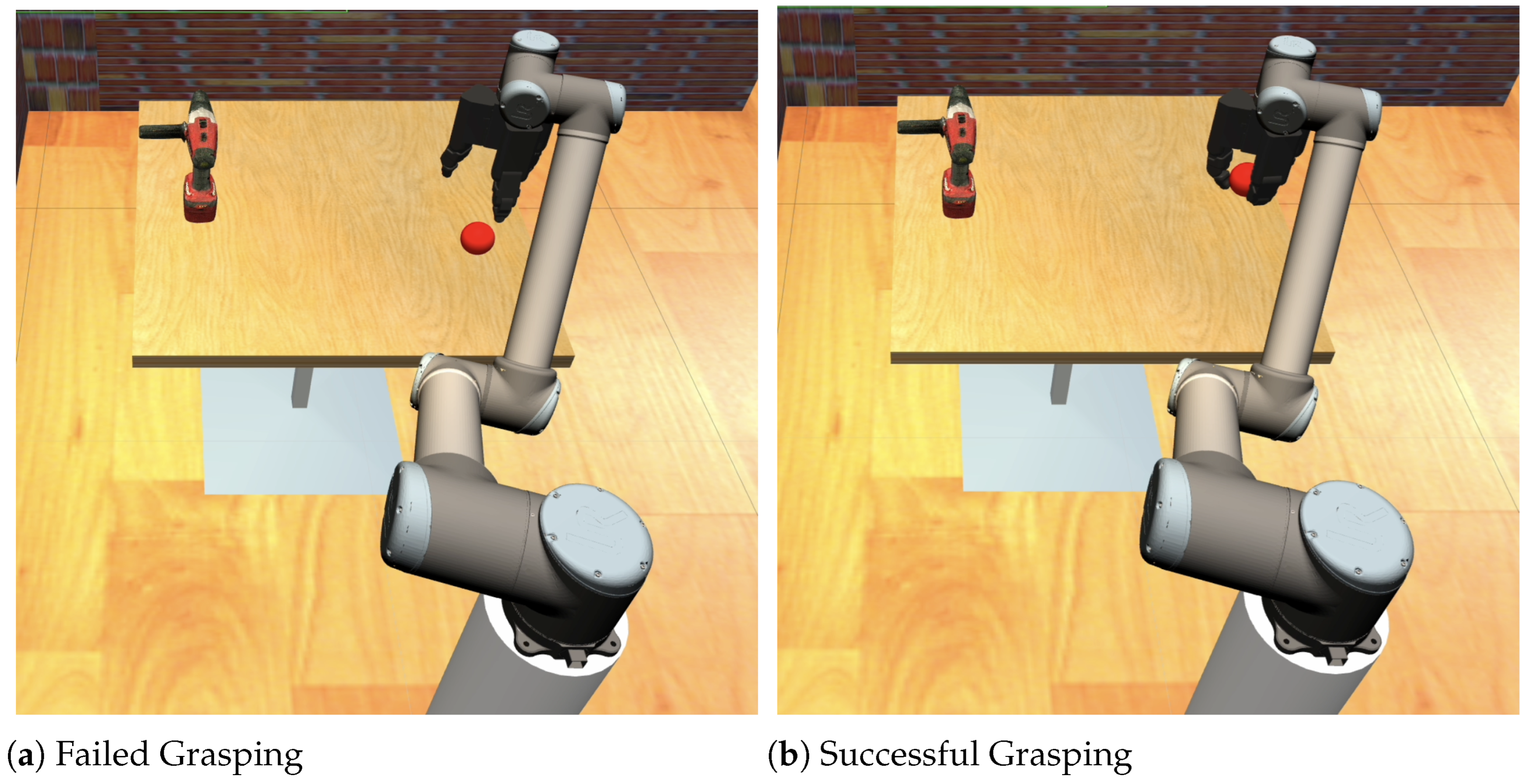
2.1. Grasp Stability Prediction in Robotics

Predicting and ensuring grasp stability remains a fundamental challenge in robotic manipulation systems. According to [36], fault diagnosis approaches in robotic systems can be broadly categorized into two principal techniques: hardware redundancy-based and analytical redundancy-based techniques. Hardware redundancy-based approaches typically involve duplicating critical system components to provide backup mechanisms when failures occur. While effective, these methods often increase system complexity, cost, and weight—making them impractical for many robotic applications, particularly those requiring agile manipulation [37].

In contrast, analytical redundancy-based methods offer more flexible solutions by utilizing mathematical and computational approaches to detect and predict failures, including model-based approaches that rely on explicit mathematical representations of the robotic system to detect deviations from expected behavior; signal-based methods that analyze patterns in sensor data to identify anomalies; knowledge-based approaches that leverage domain expertise encoded in rule-based systems; data-driven techniques that utilize machine learning to extract patterns from historical performance data; hybrid fault diagnosis systems that combine multiple approaches; and active fault diagnosis methods that deliberately perturb the system to observe its response [36].

Data-driven approaches have gained significant attention in recent years due to their ability to handle complex, non-linear systems without requiring explicit system models. These approaches leverage machine learning algorithms to extract meaningful patterns from historical performance data, enabling the prediction of potential failures before they occur [38]. Their primary advantage stems from their versatile ability to adapt to different systems and failure modes without relying on explicit, potentially complex system models or extensive domain knowledge. Machine learning algorithms have been applied to help robots learn manipulation strategies and make decisions based on multi-modal sensory information. This information typically includes visual data from cameras (processed as image features), tactile feedback, and kinematic data such as joint positions or velocities of gripper mechanisms [39]. The integration of this diverse sensory information allows robotic systems to develop more robust grasping strategies adaptable to various object geometries and environmental conditions.

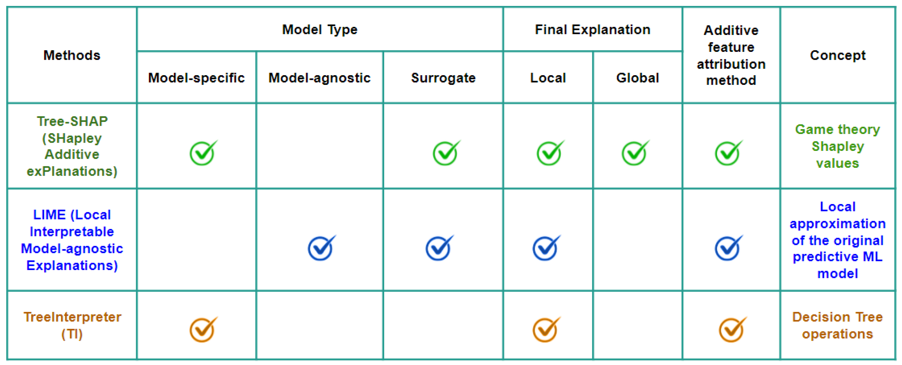
2.2. Post Hoc Explanation Methods

Post hoc explanation methods provide interpretability to black-box machine learning models by analyzing model behavior after training. As shown in Figure 1, these methods can be categorized based on several key characteristics derived from the explainable AI literature [8,40,41]. The primary dimensions for classifying post hoc explanation methods include the following:

• Model Type: Methods can be either model-specific (designed for particular model architectures) or model-agnostic (applicable to any black-box model) [20,22]. Some approaches use surrogate models that approximate the original model’s behavior in specific regions [20].
• Final Explanation: Methods provide local explanations (explaining individual predictions), global explanations (explaining overall model behavior), or both [41,42].
• Additive Feature Attribution: Some methods express explanations as a sum of feature effects [22].
• Underlying Concept: The theoretical foundation behind the explanation approach.

Tree-SHAP is a model-specific approach that provides both local and global explanations using Shapley values from game theory [23]. LIME (Local Interpretable Model-agnostic Explanations) [20] offers local explanations by creating surrogate models that approximate the original predictive model’s behavior in localized regions. TreeInterpreter (TI) [24] is designed explicitly for tree-based models and breaks down predictions into feature contributions using the internal structure of Decision Trees. Although all three methods function as additive feature attribution approaches, they employ different underlying concepts to generate explanations. In the following sections, we describe each method in detail.

2.2.1. Local Interpretable Model-Agnostic Explanations (LIME)

Local Interpretable Model-agnostic Explanations [20] is a model-agnostic approach, which means it can be applied regardless of the $ML$ model. Further, it provides individual explanations. To explain why an $ML$ model made a specific prediction for input (x), $LIME$ approximates the prediction of the ML model (f) with a linear regression explanation model (g) locally around that prediction’s (${\pi }_x$) [11]. This explanation model (g) is obtained by solving the following optimization problem that seeks a local model (g) with high fidelity of the original model (f) in the neighborhood (${\pi }_x$).

$$explaination\left(x\right)=\underset{g\in G}{argmin}L(f,g,{\pi }_x)+\Omega \left(g\right)$$

(1)

The explanation model g belongs to a family of interpretable models (G) such as Decision Trees or linear models. The goal is to minimize $L(f,g,{\pi }_x)$ while keeping the complexity of the explanation model ($\Omega \left(g\right)$) low to achieve understandable explanations [20].

2.2.2. SHAP and Tree-SHAP

SHAP is an additive feature attribution method, where the explanation is represented as a linear function, which makes it more understandable for the users [8]. Shapley values explain the model’s output of a function f as a sum of the effect ${\varphi }_i$ that each feature has contributed to the output. Based on the additive feature attribution, the explanation model of g is defined:

$$g\left(z^{\prime }\right)={\varphi }_0+\sum _{i=1}^M{\varphi }_i{z}_i^{\prime }$$

(2)

where M is the number of features, $z^{\prime }\in {\{0,1\}}^M$, and ${\varphi }_i\in \mathbf{R}$. The $z_i^{\prime }$ is equal to one if a feature is observed and equal to zero for unknown features, while the ${\varphi }_i$s are the attribution levels of features.

Also, $f\left(h_x\left(z^{\prime }\right)\right)$ is a mapping function that evaluates the effect of feature observation. Set S is the set of non-zero indexes in z, $f_x\left(S\right)=f\left(h_x\left(z^{\prime }\right)\right)=E\left[f\left(x\right)\right|x_s]$. $E\left[f\left(x\right)\right|x_s]$ is the expected value of the function conditioned on a subset S of the input features. SHAP values combine these conditional expectations with the classic Shapley values from game theory to attribute ${\varphi }_i$ values to each feature, as follows:

$${\varphi }_i=\sum _{S\subseteq N\setminus \left\{i\right\}}{\displaystyle \frac{\left|S\right|!(M-|S|-1)!}{M!}}[f_x(S\cup \left\{i\right\})-f_x\left(S\right)]$$

(3)

where N is the set of all input features [23].

SHAP interaction values, based on the Shapley interaction index from game theory [43], are included here for theoretical completeness. While our current analysis focuses primarily on individual feature attributions, we include this background as it provides important context for understanding how SHAP can be extended to capture feature interactions.

The SHAP interaction value between feature i and feature j (${\varphi }_{ij}$, where ${\varphi }_{ij}={\varphi }_{ji}$) quantifies how the combined presence of both features affects predictions beyond their individual contributions. The main effect for a feature (${\varphi }_{i,i}$) is calculated as follows:

$${\varphi }_{i,i}={\varphi }_i-\sum _{j\ne i}{\varphi }_{i,j}$$

(4)

2.2.3. TreeInterpreter (TI)

TreeInterpreter (TI) [25] generates explanations for individual predictions in tree-based models by decomposing the prediction output into feature contributions [44]. TI works by tracking the decision path taken by each data point through the tree, from the root node to the corresponding leaf node, and attributing the changes in prediction values at each split to the feature responsible for that split. Specifically, when a data point traverses from a parent node to a child node during prediction, there is typically a change in the predicted value. TI attributes this change to the feature that determined the split at that node. For each node in the decision path, TI calculates the following:

• The expected prediction value at the parent node (based on all training samples that reached that node).
• The expected prediction value at the child node the sample moves to.
• The difference between these values, which represents the contribution of the feature that defined the split.

This process can be formalized as follows. Let $f\left(x\right)$ be the decision function for a single tree, which can be decomposed into the following:

$$f\left(x\right)=C_{full}+\sum _{k=1}^{K}contrib(x,k)$$

(5)

where $C_{full}$ is the bias term (the value at the root node, representing the average prediction over the entire training dataset), $contrib(x,k)$ is the contribution of feature k for sample x, and K is the total number of features.

For each feature k used in the decision path, the contribution is calculated as the sum of prediction value changes at all nodes where feature k determines the split. For features not used in the decision path, the contribution is zero.

For Random Forest models, which consist of multiple Decision Trees, TI averages the contributions across all trees:

$$F\left(x\right)={\displaystyle \frac{1}{J}}\sum _{j=1}^J{f}_j\left(x\right)$$

(6)

$$F\left(x\right)={\displaystyle \frac{1}{J}}\sum _{j=1}^J{C}_{j}full+\sum {k=1}^K\left({\displaystyle \frac{1}{J}}\sum _{j=1}^{J}contri{b}_j(x,k)\right)$$

(7)

where J is the number of trees in the forest, $f_j\left(x\right)$ is the prediction from the j-th tree, $C_{j_{full}}$ is the bias term for the j-th tree, and $contri{b}_j(x,k)$ is the contribution of feature k in the j-th tree for sample x. This detailed decomposition makes TI particularly valuable for tree-based models, as it provides intuitive and accurate feature attributions by directly leveraging the model’s internal structure rather than approximating it.

2.3. Feature Importance in Decision Tree and Random Forest Classifiers

Since we compare the global explanations of Decision Trees (DTs) [45] and Random Forests (RFs) [46], in this section, we provide a brief review of how these explanations can be measured in different ML models.

The global explanation shows the importance of each feature (globally) on the model’s outcome over the entire training set. The explanations are based on the feature importance $\left(FI\right)$ score that measures the impact of each feature on predicting the output of ML models (either black-box or white-box models) such as RF or Logistic Regression (LR) [9,10]. However, $FI$ cannot be considered as a ‘consistent’ explainer [23]. This means that changing the model can decrease the importance of a feature despite the fact that the feature may still have a high impact on the predicted output [23]. For example, a feature may appear less important in a model due to masking effects from highly correlated features or due to the model’s specific learning algorithm, even if that feature has strong predictive power in reality [47].

In linear ML models such as LR, the output of the model is the weighted sum of input features. Therefore, these linear models provide a set of coefficients, which can be used as the $FI$ score [48]. In tree-based models such as DT and RF, the importance of each feature is measured based on the reduction in impurity criterion [49] after choosing that feature (i) to split a node (j), which is explained in Equation (8) in more detail.

The feature importance of DT models can be measured by Gini Impurity [49] or Entropy [50] for classification tasks and Mean Squared Error (MSE) [49] or Mean Absolute Error (MAE) [51] for regression tasks. Considering a binary tree built by the CART algorithm [49], the importance of node j after splitting on feature i ($n{i}_j$) is defined by calculating the reduction in node impurity ($C_j$) and weighting it by the probability ($w_j$) of reaching node j, as shown in Equation (8).

$$n{i}_j=w_j{C}_j-w_{\mathrm{left}\left(j\right)}{C}_{\mathrm{left}\left(j\right)}-w_{\mathrm{right}\left(j\right)}{C}_{\mathrm{right}\left(j\right)}$$

(8)

Here, $C_{\mathrm{left}\left(j\right)}$ and $w_{\mathrm{left}\left(j\right)}$ are the impurity and the weighted number of samples reaching the child node from the left split on node j, respectively. The same notation applies for the child node from the right split on node j ($right\left(j\right)$) [52].

Then, the importance of feature i ($f{i}_i$) is determined by adding the importance of all nodes j that are split on feature i, over the summation of node importance values for all nodes k ($n{i}_k$), as follows [52,53].

$$f{i}_i={\displaystyle \frac{{\sum }_{j:\mathrm{node}\mathrm{j}\mathrm{splits}\mathrm{on}\mathrm{feature}\mathrm{i}}n{i}_j}{{\sum }_{k\in \mathrm{all}\mathrm{nodes}\mathrm{k}}n{i}_k}}$$

(9)

Similarly, for the RF algorithm, the feature importance score ($RFf{i}_i$) is obtained by averaging over all T trees, as given by Equation (10) [46,53]:

$$RFf{i}_i={\displaystyle \frac{{\sum }_{t:\mathrm{all}\mathrm{trees}}normf{i}_{it}}{T}}$$

(10)

where $normf{i}_{it}$ is the normalized importance of feature i in tree t and has values between 0 and 1. Finally, the feature importance in $RF$ is defined by dividing the summation of normalized feature importance scores on each tree t by the total number of trees T. Therefore, features with higher values are considered more important for the model’s predictions [46,52]. This aggregation across multiple trees provides more robust feature importance estimates compared to single Decision Trees, as it reduces variance and mitigates the impact of individual tree structures on feature importance calculations [53].

2.4. Rank Similarity Metrics

To measure the similarities between ranked lists of different explanations (lists of the features that are ranked based on their contributions or impacts on the model’s output) generated by post hoc methods, we use two types of metrics [54]: correlation-based (e.g., Kendall’s Tau) and intersection-based (e.g., Rank-Biased Overlap) methods. As shown in

Table 1. Rank similarity metrics’ ranges of values and their meanings.

	$-1$	0	1
Kendall’s Tau	similar in reverse order	disjoint (no similarity)	identical (similar)
Weighted Kendall’s Tau	similar in reverse order	disjoint	identical
RBO	NA	disjoint	identical
Weighted RBO	NA	disjoint	identical

, these metrics have different ranges and interpretations. While correlation-based metrics like Kendall’s Tau range from −1 (reverse order similarity) to 1 (identical rankings), intersection-based metrics such as Rank-Biased Overlap (RBO) range from 0 (disjoint rankings) to 1 (identical rankings).

2.4.1. Kendall’s Tau Correlation Coefficient

One of the most commonly used rank correlation measures is Kendall’s Tau correlation coefficient [55]. This metric calculates the probability of two items appearing in the same order in two (conjoint) ranking lists. If the items are in the same order (identical), then correlation is strong and positive (+1), whereas the reverse order results in a strong and negative correlation (−1). Moreover, ‘randomly’ related or uncorrelated items will have a correlation coefficient of zero [56,57].

In calculating the correlations between every pair of items from two ranked lists, Kendall’s Tau assumes that the lists are conjoint (all the features are available in both lists) and there are no ties between the lists (no two items have the same rank in each of the two lists) [56]. Considering these assumptions, Kendall’s Tau ($\tau$) can be calculated as follows.

$$\tau =p_c-p_d={\displaystyle \frac{C}{P\left(n\right)}}-{\displaystyle \frac{D}{P\left(n\right)}}={\displaystyle \frac{C-D}{\frac{n(n-1)}{2}}}$$

(11)

Having n items in a ranked list, $P\left(n\right)$ is the total number of pairs. Therefore, the probability of choosing a pair of items i and j at random, if the pair have the same order in both ranked lists (concordant pairs), can be calculated as $p_c$. Similarly, the probability of discordant pairs (D) can be computed as $p_d$. Here, C is the number of concordant pairs and D is the number of discordant pairs. Despite the fact that Kendall’s Tau has been widely used in quantifying the similarities of ranked lists, this metric is inefficient for non-conjoint rankings (when some items exist in one ranked list but not in the other list) [56]. Also, it does not assign higher weights to the top items of the ranked list, meaning that it is unweighted.

We present this standard formulation (often called Tau-a) to establish the theoretical foundation of rank correlation, even though it has limitations for our specific application. In practice, feature importance rankings often contain ties (when multiple features have identical importance values) and may not be conjoint (when explanation methods prioritize different feature subsets). Therefore, in our actual implementation, we use Kendall’s Tau_b [58], which properly handles ties and provides more reliable correlation estimates for feature importance rankings in explainable AI contexts. This methodological choice maintains the conceptual strengths of rank correlation while addressing the practical challenges presented by our data.

2.4.2. Rank-Biased Overlap (RBO)

RBO (Rank-Biased Overlap) [56] handles Kendall’s Tau issues. RBO measures the similarity between two rankings even if they are incomplete (which, in that case, it needs to support non-conjoint rankings) and at any depth of the lists. Looking at RBO from the set intersection (overlap) perspective, the overall idea behind RBO is to ‘bias the proportional overlap at each depth by a convergent series of weights’ (a geometric series with a finite sum as formulated in Equation (12)). In other words, RBO can be calculated by averaging the proportion of items overlapping while increasing the depths d as follows.

$$\sum _{d=1}^{\infty }{p}^{(d-1)}={\displaystyle \frac{1}{1-p}}$$

(12)

Having two infinite ranking lists S and T, $S_i$ and $T_i$ refer to their elements at rank i. Therefore, the size of the intersection (overlap) between these two ranking lists at each depth d ($I_{S,T,d}$) can be measured as follows.

$$X_{S,T,d}=\left|I_{S,T,d}\right|$$

(13)

$$I_{S,T,d}=S_{:d}\cap T_{:d}$$

(14)

where $S_{:d}$ and $T_{:d}$ refer to the elements that appear in the intersections of lists S and T, from position 1 to d. Defining $A_d$ as the proportion of items overlapping up to depth d, the average of the overlap ($AO(S,T,k)$) can be formulated as shown in Equations (15) and (16).

$$A_d={\displaystyle \frac{X_{S,T,d}}{d}}$$

(15)

$$AO(S,T,k)={\displaystyle \frac{1}{k}}\sum _{d=1}^k{A}_d$$

(16)

where k is the evaluation depth. After having the average of overlaps at each depth and considering w to be a vector of weights and $w_d$ as the weight at position d, the similarity between two ranked lists S and T can be measured using Equation (17) [56].

$$SIM(S,T,w)=\sum _{d=1}^{\infty }{w}_d·A_d$$

(17)

If w is a convergent vector of weights (with finite sum as formulated in Equation (12)), Rank-Biased Overlap can finally be computed [56] using

$$RBO(S,T,p)=(1-p)\sum _{d=1}^{\infty }{p}^{(d-1)}·A_d$$

(18)

Therefore, RBO ranges from 0 to 1, where 0 means the ranked lists are disjoint and 1 means they are identical. In Equation (18), the degree of top (d) weighted-ness of RBO is defined by parameter p. Thus, the smaller value of p indicates that top ranked items have more weights in measuring similarities by RBO compared to the items in the bottom of the lists. Similarly, for values of p closer to 1, the weights become arbitrarily flat [56] and RBO becomes unweighted.

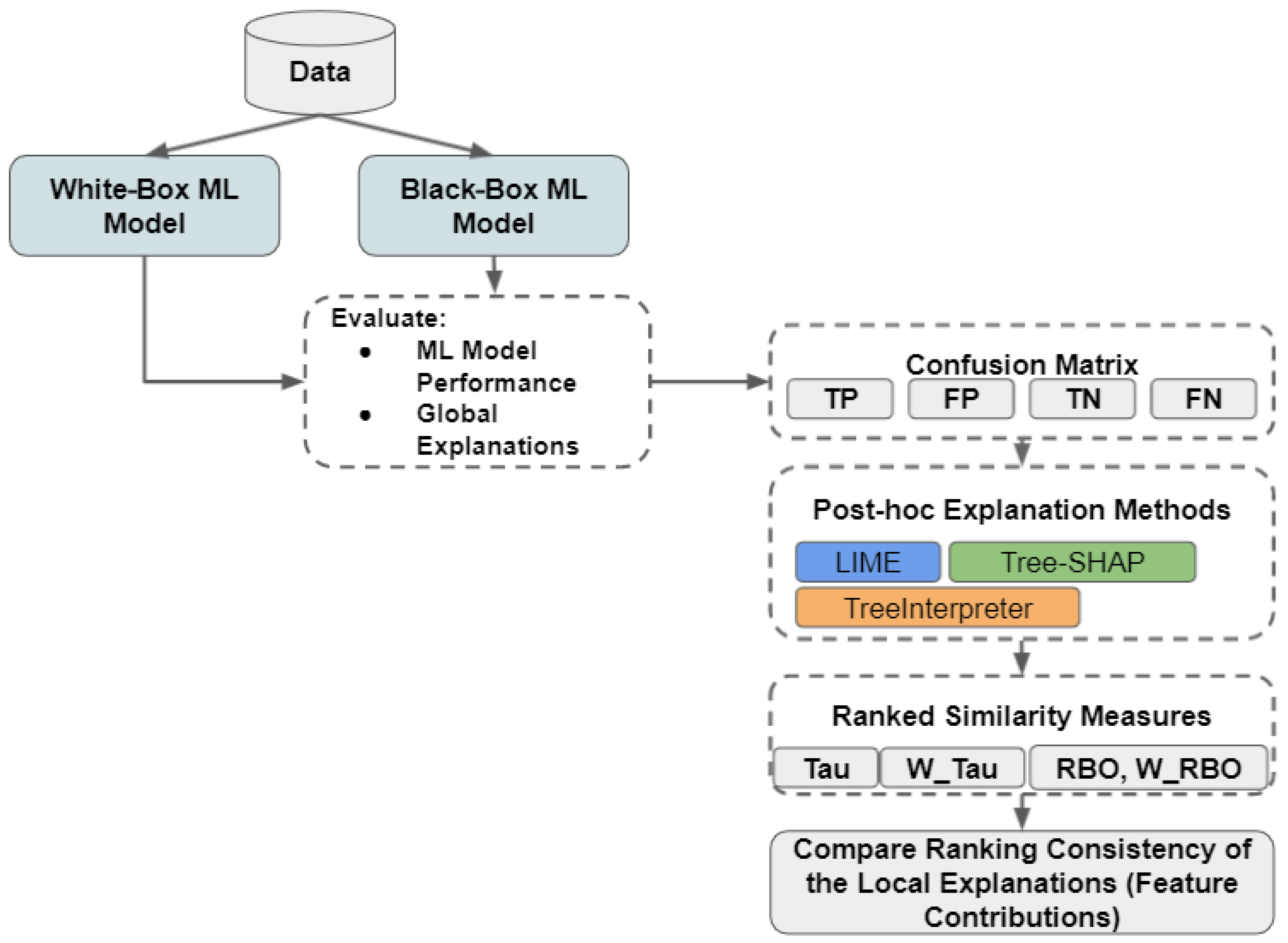
3. Methodology: Application to Robotics Grasping Failure Detection

In this work, we train and compare two different models on grasp failure simulation data, a white-box model (Decision Tree classifier [9]), which is inherently interpretable, and a black-box model (Random Forest classifier [46]) with high accuracy and no explanations about the prediction results. To explain individual predictions, we use Tree-SHAP [23], LIME [20], and TreeInterpreter (TI) [24,25] explanation methods to provide local explanations for any sample of data. Figure 2 depicts the flow of our methodology, starting with learning predictive models for failure and then generating explanations for predicted failures. After evaluating the prediction results of both white-box and black-box models, we apply the explanation method to generate local explanations for each record in sub-samples of the test set (depending on the classification output, namely, False Negative (FN), True Negative (TN), False Positive (FP), and True Positive (TP)). Then, we use four ranking similarity metrics (Kendall Tau [55], Weighted Kendall Tau [59], RBO, and Weighted RBO [56]) to measure the similarity between the top 3 feature contributions generated by each explanation method. These ranking similarity metrics are applied to compare the top 3 feature importance lists generated by each explanation method for every individual instance in the test set. For each instance and each pair of explanation methods (Tree-SHAP vs. LIME, Tree-SHAP vs. TreeInterpreter, and LIME vs. TreeInterpreter), we calculate all four similarity metrics, resulting in a distribution of similarity values for each classification category. We then report the median of these distributions as a robust measure of central tendency that is less affected by outliers than the mean. The combination of correlation-based metrics (Kendall’s Tau variants) and intersection-based metrics (RBO variants) provides complementary perspectives on ranking similarity. While correlation-based metrics focus on order agreement, intersection-based metrics emphasize the overlap of elements regardless of their exact positions. Furthermore, the weighted variants of both types of metrics assign greater importance to agreement on top-ranked features, which is particularly valuable when analyzing feature importance rankings where the most influential features have disproportionate impact on predictions. It is important to note that these metrics assess the similarity of rankings rather than the magnitude of feature contributions, focusing on the relative importance ordering rather than absolute importance values. This approach is appropriate for comparing explanation methods that may use different scales for quantifying feature importance.

To evaluate the rankings of explanation methods, we examine the top 3 features identified by each method. We focus on the top 3 features because these typically account for the majority of the contribution to predictions in our analysis (representing approximately 70–85% of total feature importance across methods) while maintaining a manageable comparison scope. This approach aligns with common practice in feature importance analysis [60,61], where a small subset of dominant features often drives predictions. For robotic grasp applications specifically, focusing on the top contributors provides actionable insights for engineers seeking to improve grasp reliability by addressing the most influential factors. After initial exploration with various thresholds (top 2 through top 5), we found the top 3 to offer the optimal balance between capturing essential information and enabling meaningful comparisons across methods.

We used a simulated robotic grasp dataset [62,63], which records the performance of a robot’s arm with three fingers, including information about joints’ position, velocity, effort (torque) of each finger, and stability of the grasp for an object. The simulated environment utilizes the Gazebo physics engine with ROS integration to accurately model the dynamics of the Shadow Robot Hand. This simulation environment implements realistic physical properties, including gravity, friction, and object inertia, while modeling the hand’s actuators, sensors, and control systems. The Shadow Robot Company validated this simulation environment against their physical robot to ensure high fidelity between simulated and real-world behavior [62]. While the simulation captures the most relevant dynamics, certain simplifications were necessary for computational efficiency. These include idealized contact models that may not fully capture all deformation properties of real objects, simplified friction models, and perfect sensor readings without the noise typically present in physical sensors. These simplifications may affect generalizability, particularly in scenarios where tactile feedback quality or surface property variations significantly impact grasp outcomes. However, the large-scale nature of the dataset (nearly 1 million grasp attempts) helps mitigate these limitations by capturing a diverse range of grasping scenarios that would be impractical to reproduce in physical experiments. Additionally, the focus of our study is on comparing explanation methods rather than absolute performance prediction, making the simulation data appropriate for this purpose while acknowledging that transfer to physical systems would require validation with real-world experiments.

The grasping dataset was obtained from Shadow’s Smart Grasping System [35] simulation with the ROS [64] and Gazebo [65] environment using the Smart Grasping Sandbox, and containing three 3-DOF fingers, shown in Figure 3. These measurements were collected into features named after the combination of hand (only Hand 1 is used), finger, joint, and either position, velocity, or effort, as summarized in the following list:

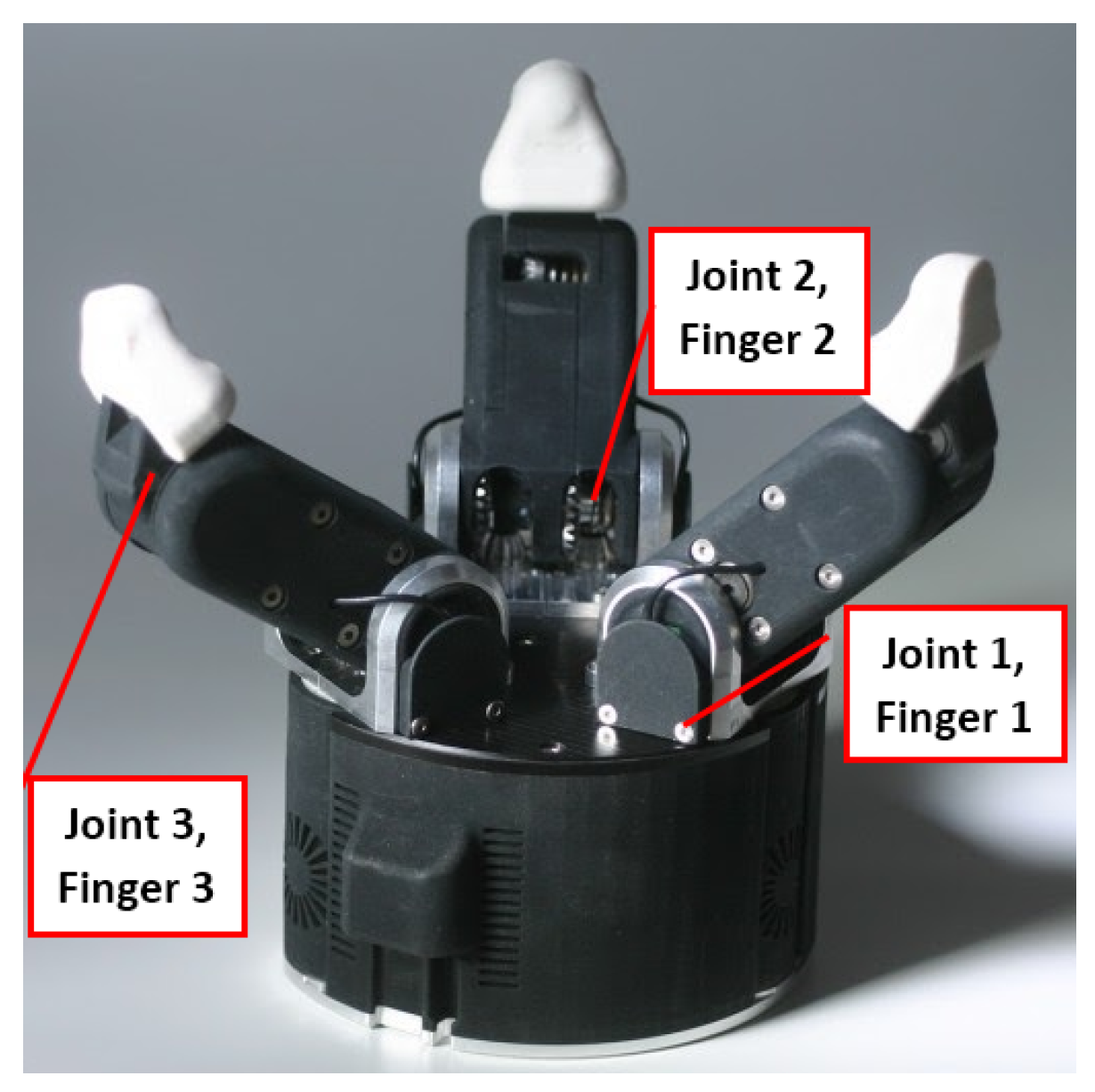
• $H1$: Hand 1, indicating the only hand used in the simulation.
• $F1,F2,F3$: Fingers on the hand, where each finger has three joints.
• $J1,J2,J3$: Joints in each finger, with each joint having measurements for position ($pos$), velocity ($vel$), and effort ($effort$).

Hence, $H1FjJk$ indicates joint k of Finger j of Hand 1.

Table 2. Notation of input features.

Feature	Definition
$H_1\_F_1{J}_1\_eff$	effort in joint 1 in finger 1
$H_1\_F_1{J}_1\_vel$	velocity in joint 1 in finger 1

provides more details about feature notations and definitions that were used in this simulation. The output is discretized to 1 for a stable grasp and 0 for an unstable grasp, with simulation output examples are shown in Figure 4.

Following the recommendation in [62], the joint position was excluded from the features. This is because the shape of the hand is object-specific; however, our aim in this paper is to predict the quality of the grasp in an object-agnostic manner. As a result, 18 input features, which measure effort (torque) and velocity of each joint in all of the three fingers, and a grasp quality feature, which was labeled as Success or Failure (as the target label), were used in training every ML model. Table 2 provides more details about feature notations and definitions that were used in this dataset.

The dataset has 992,641 records of grasps and 28 features, with 448,046 records (45% of data) labeled as successful (stable) grasps and 544,595 records (55% of data) labeled as failed (unstable) grasps, with simulation examples shown in Figure 4.

To evaluate the rankings of explanations, we employ a comprehensive approach utilizing multiple complementary assessment techniques. Correlation-based metrics, specifically Kendall’s Tau and Weighted Kendall’s Tau, measure the agreement in the ordering of feature rankings across explanation methods. While these metrics provide valuable insights into ranking similarity, they require conjoint rankings and may be sensitive to minor variations. To address these limitations, we also use intersection-based metrics such as Rank-Biased Overlap (RBO) and Weighted RBO, which measure the overlap between rankings at different depths and can handle non-conjoint rankings, thereby offering more robust comparison capabilities. Performance evaluation constitutes another important dimension of our assessment, where we examine the computational efficiency of each explanation method by measuring their execution time across different model types. Finally, we analyze the consistency of explanation methods across different classification outcomes (True Positive, True Negative, False Positive, and False Negative), which provides insights into the robustness of these methods across various prediction scenarios. These multiple evaluation dimensions together offer a comprehensive framework for assessing and comparing post hoc explanation methods for robotic grasp failure prediction.

For each of these classification outcome categories (TP, TN, FP, FN), we use the complete set of examples from the test set. Specifically, for the Decision Tree classifier, this resulted in 43,272 True Negative instances, 35,703 True Positive instances, 18,667 False Negative instances, and 1622 False Positive instances. Similarly, for the Random Forest classifier, we analyzed 43,057 True Negative instances, 36,564 True Positive instances, 17,806 False Negative instances, and 1837 False Positive instances. This comprehensive approach ensures that our analysis captures the full variability in explanations across different classification outcomes without introducing selection bias.

4. Results

4.1. Experimental Setup

To conduct our experiments, we used the Scikit-learn library [66] for building the models. Scikit-learn implements an optimized version of the CART (Classification and Regression Trees) algorithm [49] for DT models. For assessing overall model performance, we performed an initial cross-validation with 5 folds (80% training, 20% validation) and reported metrics averaged across validation folds. Following this, we focused on the best validation split for our main experiments. All experiments were conducted on a 2.20 GHz Intel Core i7 virtual machine with 8 GB of RAM running on Google Cloud Platform.

To ensure optimal model performance, we conducted hyperparameter tuning using grid search while evaluating the Area Under the Curve (AUC) metric on the validation set. For the Random Forest classifier, we explored combinations of the following hyperparameters: number of estimators [5, 20, 100, 200, 300], maximum features [‘log2’, ‘sqrt’], splitting criterion [‘entropy’, ‘gini’], maximum depth [2, 3, 5, 8], minimum samples for split [2, 10], and minimum samples per leaf [1, 5, 10]. The optimal Random Forest configuration used 300 estimators with ‘sqrt’ maximum features, ‘gini’ criterion, maximum depth of 8, minimum samples split of 10, minimum samples leaf of 5, and random state of 123. For the Decision Tree classifier, we tuned maximum features [‘log2’, ‘sqrt’], criterion [‘entropy’, ‘gini’], maximum depth [2, 3, 5, 8], minimum samples split [2, 10, 50, 100], and minimum samples leaf [1, 5, 10]. The final Decision Tree model used ‘log2’ maximum features, ‘entropy’ criterion, maximum depth of 8, minimum samples split of 2, minimum samples leaf of 5, and random state of 123. These optimized configurations ensured that our models achieved their best possible performance while maintaining good generalization capabilities.

It is worth noting that we did not apply any outlier detection or removal techniques to the simulated dataset. Since the data were generated through controlled simulation of the Smart Grasping System, extreme values were considered legitimate outcomes of the physics-based simulation rather than errors. Additionally, we confirmed that the dataset contained no missing values, eliminating the need for imputation strategies that might affect model performance or interpretability. This approach preserves the full range of simulated grasping behaviors, including edge cases that might be important for understanding failure modes in real-world applications.

In our implementation of RBO and Weighted RBO metrics, we use a parameter value of p = 0.8, following recommendations in [56] for applications where top-ranked items should receive substantial but not overwhelming emphasis. This value provides appropriate sensitivity to differences in the ordering of the most important features while still accounting for lower-ranked features. The choice of p = 0.8 balances our interest in feature ranking agreement across both highly influential features (which have the greatest impact on model predictions and potential corrective actions) and moderately important features (which provide context and may become more significant in different grasping scenarios). We conducted a sensitivity analysis with p values ranging from 0.7 to 0.9 and found that while the absolute similarity values changed slightly, the relative patterns remained consistent, supporting the robustness of our findings.

4.2. ML Model Performance Comparison

Before addressing our research questions, we first compare the performance of the two ML models used in this study. All results presented are obtained from 5-fold cross-validation and include standard performance metrics: accuracy, area under the ROC curve (AUC), precision, recall, and F1 score. All metrics are in the range $[0,1]$, with higher values indicating better performance.

Table 3. Mean (and standard deviation) of ML model performance, Random Forest (black-box) vs. Decision Tree (white-box).

Metric	Random Forest	Decision Tree
Accuracy	0.8020 (±0.0001)	0.7947 (±00030)
F1	0.7879 (±0.0004)	0.7816 (±0.0062)
Precision	0.9530 (±0.0015)	0.9369 (±0.0124)
Recall	0.6715 (±0.0013)	0.6707 (±0.0151)
AUC	0.8712 (±0.0002)	0.8524 (±0.0053)

presents the mean and standard deviation of these metrics for both models. The Random Forest classifier achieves superior performance across all metrics compared to the Decision Tree classifier, with an AUC of 0.8712 (±0.0002) versus 0.8524 (±0.0053). This performance advantage is expected since RF is an ensemble method aggregating predictions from multiple Decision Trees, reducing variance and improving generalization. However, this enhanced predictive power comes at the cost of increased model complexity and reduced inherent interpretability, further motivating the importance of using effective post hoc explanation methods.

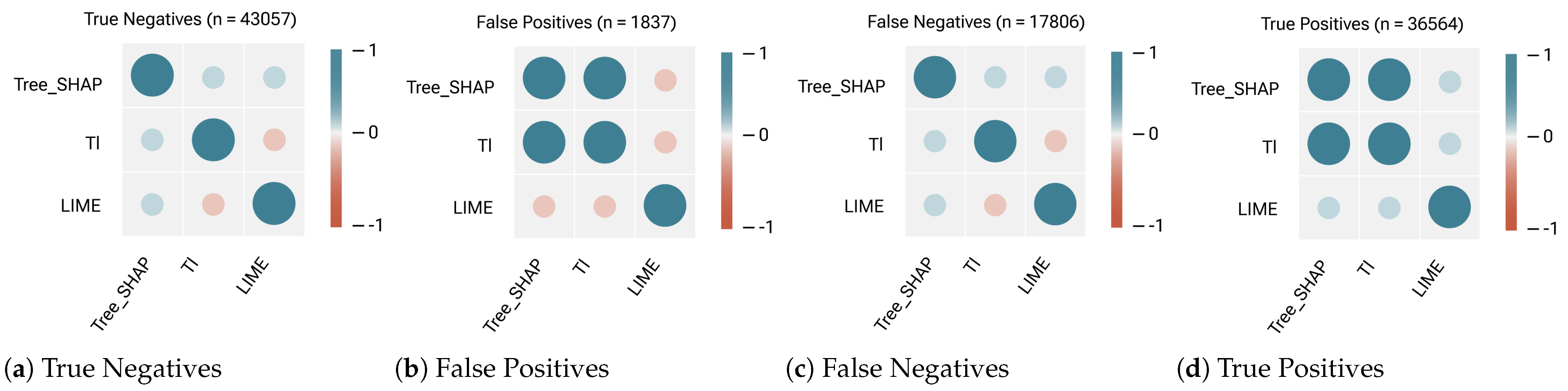
4.3. RQ1: Do the Explanation Methods Agree on Selecting the Most Responsible Feature for Grasp Failures?

To answer our first research question, we analyzed the local explanations generated by Tree-SHAP, LIME, and TreeInterpreter for individual test cases across different classification outcomes. Figure 5 and Figure 6 illustrate feature contributions for a representative True Positive case from the Random Forest and Decision Tree models, respectively.

For the Random Forest model (Figure 5), we observed moderate agreement among the methods regarding the most influential features. Tree-SHAP identifies joint 1’s effort in fingers 1 and 3 as the primary contributors to grasp failure prediction. TreeInterpreter prioritizes joint 1’s effort in finger 3, while LIME highlights joint 1’s effort in finger 1. Despite these variations in exact ranking, all three methods consistently identify effort (torque) in the first joints of the first and third fingers as critical factors.

For the Decision Tree model (Figure 6), Tree-SHAP and TreeInterpreter show strong agreement, both identifying joint 1’s effort in finger 3 as the most significant feature. LIME, however, selects joint 1’s effort in finger 1 as the primary contributor. This suggests that model complexity affects the consistency of explanations, with simpler models showing more agreement between Tree-SHAP and TreeInterpreter than more complex ones.

The global feature importance analysis in Figure 7 corroborates these findings, showing that both models prioritize joint 1’s effort across different fingers. This consistency in identifying the first joint’s effort as crucial aligns with the mechanical principles of robotic grasping, where establishing initial contact with objects using joint 1 is fundamental to successful manipulation. Based on these observations, we conclude that while the explanation methods do not always agree on the exact ranking order of features, they demonstrate substantial consensus in identifying the most responsible features for grasp failures, particularly focusing on the effort applied at critical joints.

The consistently lower agreement between LIME and the other explanation methods (Tree-SHAP and TreeInterpreter) warrants further discussion. This discrepancy likely stems from fundamental differences in how LIME generates explanations compared to the tree-specific methods. LIME creates a local surrogate model by sampling around each prediction instance and fitting a simpler, interpretable model to these synthetic samples [20]. This approach can be sensitive to sampling strategy, kernel width, and the complexity of the surrogate model. In contrast, Tree-SHAP and TreeInterpreter directly analyze the internal structure of tree-based models without requiring sampling or surrogate modeling. The sampling nature of LIME introduces stochasticity that may explain some inconsistency with the deterministic tree-specific methods. Additionally, LIME’s linear surrogate models may struggle to capture complex non-linear relationships that are naturally represented in tree structures and readily identified by Tree-SHAP and TreeInterpreter. This finding suggests that for tree-based models specifically, the model-specific explanation methods may provide more consistent feature importance rankings than model-agnostic approaches like LIME, highlighting the value of leveraging model structure when available.

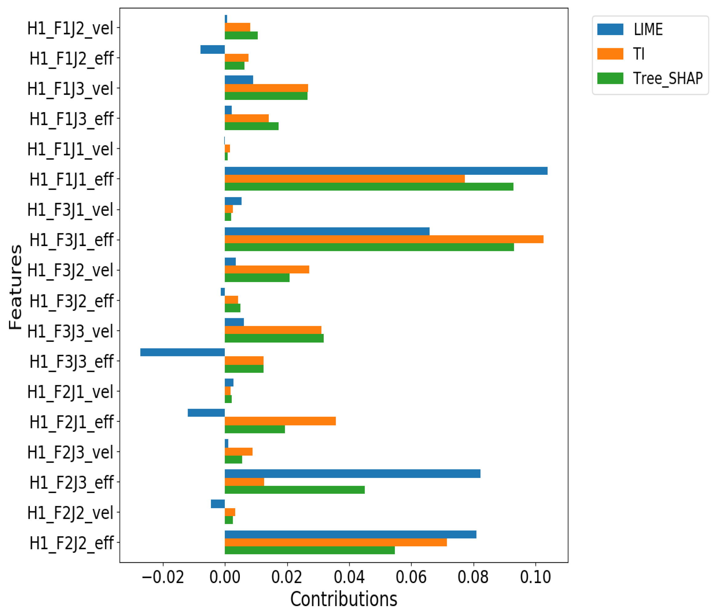
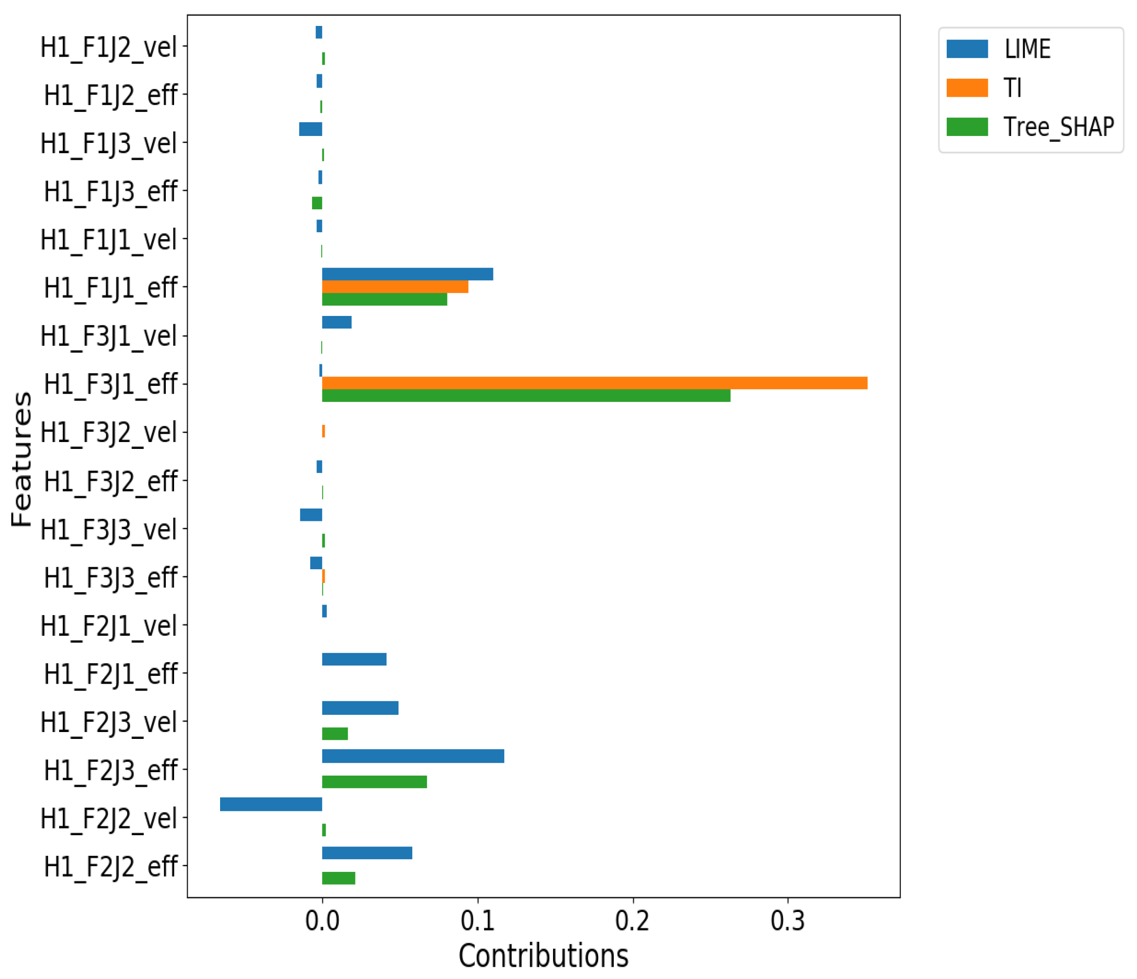
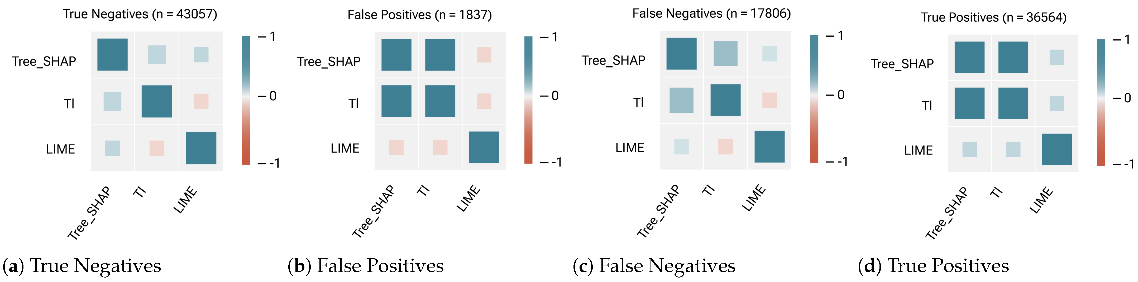
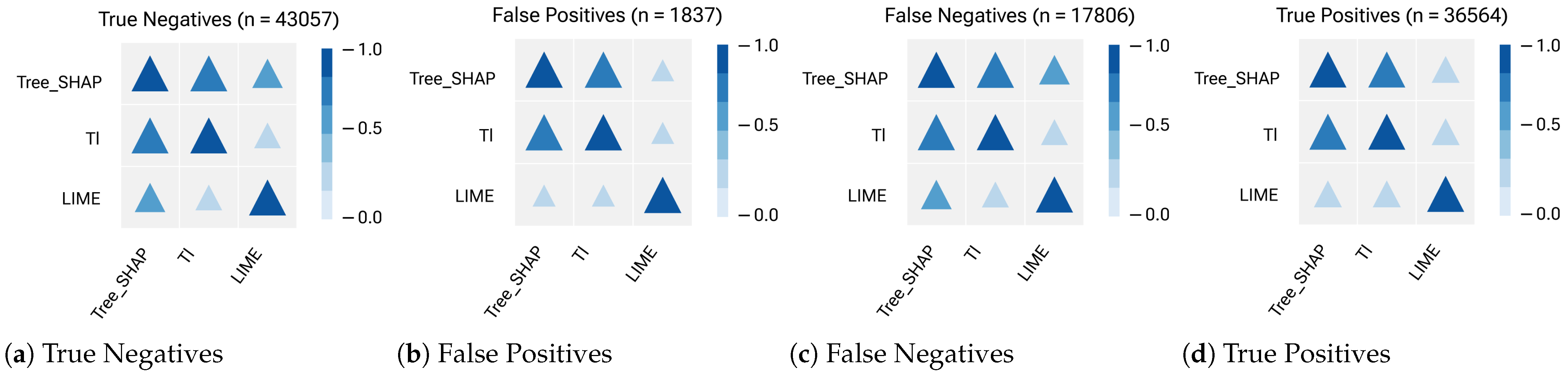
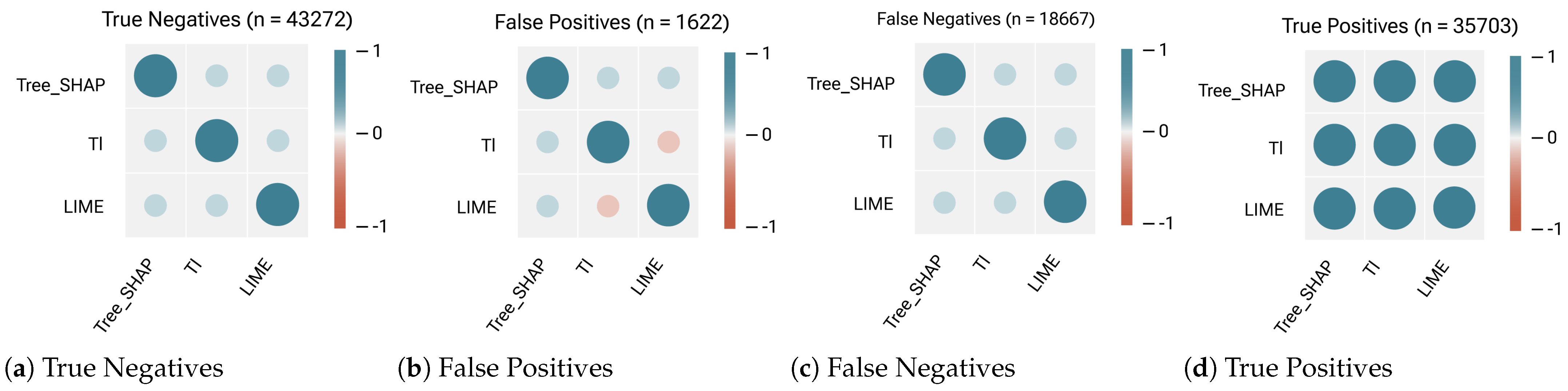
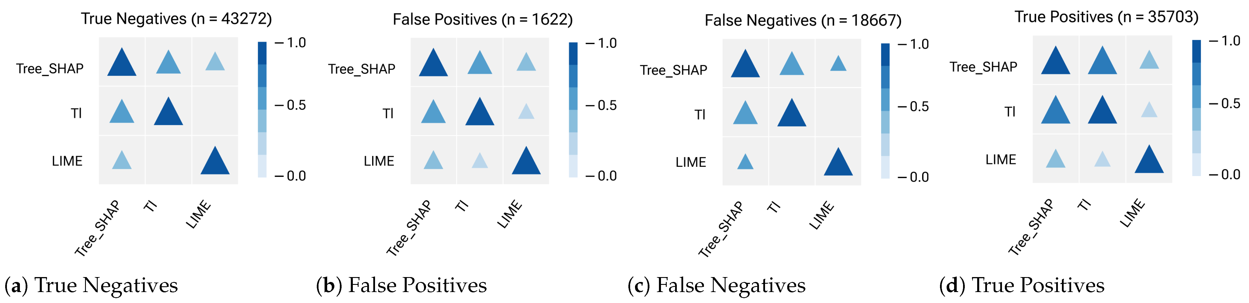
4.4. RQ2: How Similar Are Their Results on Ranking Important Features and Their Contributions in Explaining the Failures?

To quantitatively assess the similarity between feature importance rankings produced by different explanation methods, we employed both correlation-based metrics (Kendall’s Tau and Weighted Kendall’s Tau) and intersection-based metrics (RBO and Weighted RBO).

Table 4. Comparing explanations for Decision Tree and Random Forest Classifiers based on ranking-similarity (median). Note: RBO and Weighted RBO range over [0, 1]. Kendall Tau and Weighted Kendall Tau range over [−1, 1].

True Negatives
	Decision Tree				Random Forest
	Kendall Tau	Weighted K-Tau	RBO	Weighted RBO	Kendall Tau	Weighted K-Tau	RBO	Weighted RBO
Tree-SHAP & TI	0.3	0.2	0.7	0.7	0.3	0.5	0.8	0.8
Tree-SHAP & LIME	0.3	0.2	0.3	0.2	0.3	0.2	0.6	0.3
LIME & TI	0.3	0.2	0.0	0.0	−0.3	−0.4	0.4	0.2
False Negatives
	Decision Tree				Random Forest
	Kendall Tau	Weighted K-Tau	RBO	Weighted RBO	Kendall Tau	Weighted K-Tau	RBO	Weighted RBO
Tree-SHAP & TI	0.3	0.2	0.7	0.7	0.3	0.5	0.9	0.8
Tree-SHAP & LIME	0.3	0.2	0.3	0.2	0.3	0.2	0.6	0.3
LIME & TI	0.3	0.2	0.0	0.0	−0.3	−0.4	0.4	0.2
True Positives
	Decision Tree				Random Forest
	Kendall Tau	Weighted K-Tau	RBO	Weighted RBO	Kendall Tau	Weighted K-Tau	RBO	Weighted RBO
Tree-SHAP & TI	1	1	0.9	0.8	1	1	0.9	0.8
Tree-SHAP & LIME	1	1	0.4	0.2	0.3	0.5	0.4	0.2
LIME & TI	1	1	0.3	0.2	0.3	0.5	0.4	0.2
False Positives
	Decision Tree				Random Forest
	Kendall Tau	Weighted K-Tau	RBO	Weighted RBO	Kendall Tau	Weighted K-Tau	RBO	Weighted RBO
Tree-SHAP & TI	0.3	0.2	0.6	0.7	1	1	0.9	0.8
Tree-SHAP & LIME	0.3	0.3	0.4	0.2	−0.3	−0.4	0.3	0.2
LIME & TI	−0.3	−0.2	0.3	0.2	−0.3	−0.4	0.3	0.2

summarizes these similarity measures for the Decision Tree and Random Forest models, respectively, across different classification outcomes.

To facilitate the interpretation of our similarity metrics, we adopt established benchmarks from the rank correlation literature [56,57] adapted to explainable AI contexts. For Kendall’s Tau and Weighted Kendall’s Tau, values above 0.7 indicate strong agreement, 0.3 to 0.7 suggest moderate agreement, and values below 0.3 represent weak agreement. For RBO and Weighted RBO, values above 0.8 indicate strong similarity, 0.5 to 0.8 represent moderate similarity, and values below 0.5 suggest low similarity. These interpretations account for the inherent variability expected when comparing different explanation approaches across diverse model architectures. While perfect agreement (Tau = 1, RBO = 1) would indicate complete consistency across methods, even moderate agreement is noteworthy given the fundamental differences in how these explanation techniques derive feature importance.

In contrast, the agreement between LIME and the other methods is considerably weaker. When comparing LIME with Tree-SHAP for the RF model, correlations range from moderately positive (+0.3) to negative (−0.3), with the latter indicating reverse rankings. Similarly, comparisons between LIME and TreeInterpreter show negative correlations in several cases, suggesting fundamental differences in their approach to feature attribution.

For the Random Forest model (Table 4 and Figure 8, Figure 9, Figure 10 and Figure 11), Tree-SHAP and TreeInterpreter demonstrate the highest agreement, with perfect correlation (median = +1) for True Positive and False Positive cases. This strong consistency is maintained across intersection-based metrics, with RBO values of 0.9 for these classification outcomes. The similarity between these methods remains relatively high even for True Negative and False Negative cases (median Kendall’s Tau = +0.3, RBO = 0.8).

For the Decision Tree model (Table 4 and Figure 12, Figure 13, Figure 14 and Figure 15), all three explanation methods show perfect agreement in the True Positive category, with Kendall’s Tau and Weighted Kendall’s Tau both at +1. This unanimous consensus does not extend to other classification outcomes, where correlations drop significantly (median around +0.3 or −0.3). Notably, the RBO between LIME and TreeInterpreter for True Negative and False Negative cases is 0, indicating completely disjoint rankings.

The intersection-based metrics (RBO and Weighted RBO) generally yield higher similarity values than correlation-based metrics, suggesting that while explanation methods may disagree on the exact ordering of features, they tend to include similar important features in their rankings. Weighted versions of both metrics, which place greater emphasis on top-ranked features, sometimes show different patterns from their unweighted counterparts, highlighting the importance of considering ranking position when evaluating explanation similarity.

These findings reveal that ranking similarity varies substantially depending on the explanation method, model type, and classification outcome. Tree-SHAP and TreeInterpreter generally produce more consistent rankings with each other than either does with LIME, particularly for the Random Forest model. The highest consensus occurs for True Positive cases, suggesting that explanation methods are most aligned when explaining correct failure predictions.

4.5. RQ3: How Does the Choice of ML Model (Decision Tree vs. Random Forest) Affect Feature Importance Rankings?

To address whether feature importance rankings are model-dependent, we compared global feature importance rankings between the Decision Tree and Random Forest models (Figure 7) and analyzed how local explanations differ between these models for identical test cases.

Figure 7 reveals both commonalities and differences between the models. Both identify joint 1’s effort in finger 3 as the most important feature, establishing fundamental agreement on the primary factor in grasp failure prediction. However, they diverge on subsequent rankings, with RF prioritizing joint 1’s effort in finger 1 followed by joint 2’s effort in finger 2, while DT ranks joint 1’s effort in finger 1 but places joint 1’s effort in finger 2 third. This partial agreement suggests that while core mechanical principles remain relevant regardless of model choice, the specific learning algorithm influences which secondary features are deemed important.

This pattern extends to local explanations as well. Comparing Figure 5 and Figure 6, we observe that explanations generated for the same test case differ between models, even when using the same explanation method. For instance, Tree-SHAP applied to the RF model identifies joint 1’s effort in finger 1 as the most important feature, while the same method applied to the DT model highlights joint 1’s effort in finger 3. These differences reflect how each model learns from the training data and constructs its decision boundaries.

The similarity metrics in Table 4 further support the model dependency of feature rankings. The patterns of agreement between explanation methods differ markedly between models. Most notably, in True Positive cases, all three methods agree perfectly for the DT model (Kendall’s Tau = +1) but show varying levels of agreement for the RF model, where only Tree-SHAP and TreeInterpreter achieve perfect correlation.

4.6. RQ4: How Do Different Explanation Methods Compare in Terms of Computational Efficiency?

We evaluated computational efficiency across both ML models to address the practical implications of using these explanation methods in real-world robotic applications.

Table 5. Comparing the average run-time (per instance, in seconds) of three post hoc explanation methods (Tree-SHAP, TreeInterpreter and LIME) between two ML models (Decision Tree and Random Forest classifiers).

	Tree-SHAP (s)	TreeInterpreter (s)	LIME (s)
Decision Tree	0.00024	0.00001	3.33447
Random Forest	0.07646	0.00234	4.66648

and Figure 16 present the average execution time per instance for each explanation method applied to the Decision Tree and Random Forest models.

TreeInterpreter demonstrates superior computational efficiency, requiring only 0.00001 s per instance for the DT model and 0.00234 s for the RF model. In contrast, Tree-SHAP requires 0.00024 s for DT and 0.07646 s for RF, while LIME is significantly more resource-intensive at 3.33447 s for DT and 4.66648 s for RF. These differences are particularly notable for the more complex RF model, where TreeInterpreter is approximately 33 times faster than Tree-SHAP and approximately 2000 times faster than LIME.

The scaling behavior of these methods with increasing model complexity provides additional insight. When moving from DT to RF, Tree-SHAP’s execution time increases by a factor of 318, while TreeInterpreter’s increases by a factor of 234. LIME shows the smallest relative increase (only 1.4 times slower) but has the highest absolute computation time for both models. This indicates that TreeInterpreter offers the fastest absolute performance and scales more efficiently with model complexity than Tree-SHAP. These findings have significant implications for real-time robotic applications, where explanation latency could affect system responsiveness and user experience. TreeInterpreter’s exceptional efficiency makes it particularly suitable for time-sensitive contexts, while LIME’s substantial computation requirements might limit its applicability in real-time scenarios despite its model-agnostic advantages.

In conclusion, our findings confirm that feature importance rankings are indeed model-dependent, with differences arising from the underlying model architecture, learning algorithm, and complexity. While there is some consistency in identifying the most critical explaining features across models—particularly those with clear mechanical significance—the specific rankings and attribution values vary substantially. This underscores the importance of considering both model choice and explanation method when interpreting and applying explanations in robotic grasping applications.

5. Conclusions

Robots that perform high-risk tasks can significantly benefit from predicting forthcoming failures. Furthermore, especially in robot–human collaboration cases, there is a critical need to explain failure predictions. In this paper, we compared post hoc explanation methods for robotic grasp failure prediction using white-box (Decision Tree) and black-box (Random Forest) ML models. Our findings reveal that explanation methods vary in their agreement on identifying essential features, with Tree-SHAP and TreeInterpreter showing stronger consistency with each other than with LIME. This consistency is particularly evident in True Positive cases, where perfect agreement (correlation = +1) was observed across all methods for the Decision Tree model. The intersection-based metrics (RBO) demonstrated that even when considering overlapping features at different depths, Tree-SHAP and TreeInterpreter maintain higher similarity (0.8–0.9) than their similarity with LIME. The choice of ML model significantly impacts the consistency of explanations, with the simpler Decision Tree model yielding more consistent explanations across methods in True Positive cases. However, the black-box Random Forest model provides superior prediction performance (AUC = 0.8712) while maintaining reasonable explainability through post hoc methods, particularly Tree-SHAP and TreeInterpreter. From a practical implementation perspective, TreeInterpreter offers a significant advantage in computational efficiency, being approximately 24 times faster than Tree-SHAP and over 2000 times faster than LIME for the Random Forest model. This makes TreeInterpreter particularly suitable for real-time robotic applications where rapid explanation generation is crucial. Our analysis also identified that effort in joint 1 across fingers 1 and 3 plays a critical role in grasp failures, a finding consistent with mechanical design principles. This demonstrates how explainable ML approaches can provide insight into failure mechanisms, even in complex robotic systems.

Future work should address several limitations of this study. Although we used a comprehensive simulation dataset, validation with experimental data from real robotic systems is essential to confirming the generalizability of these findings. Furthermore, investigating how these explanation methods perform with other ML models, such as deep learning approaches, would provide broader insights into their applicability. Future work could extend this analysis to different hand structures to investigate how the consistency of explanation methods scales with increasing degrees of freedom and mechanical complexity. Real-time implementation of these explanation methods deserves further investigation, particularly exploring hardware acceleration or approximation techniques that could make even more computationally intensive methods viable for online robotic applications. Another promising direction is developing hybrid explanation approaches that combine the computational efficiency of TreeInterpreter with the theoretical guarantees of Tree-SHAP. Additionally, developing metrics to evaluate the human interpretability of these explanations would enhance their practical utility in collaborative human–robot settings. Finally, exploring how explanation methods could guide automated corrective actions in response to predicted failures would close the loop between explanation and action, potentially enabling self-improving robotic grasping systems.

References

1. Kitagawa, S.; Wada, K.; Hasegawa, S.; Okada, K.; Inaba, M. Multi-stage learning of selective dual-arm grasping based on obtaining and pruning grasping points through the robot experience in the real world. In Proceedings of the 2018 IEEE/RSJ International Conference on Intelligent Robots and Systems (IROS), Madrid, Spain, 1–5 October 2018; IEEE: New York, NY, USA, 2018; pp. 7123–7130. [Google Scholar]
2. Della Santina, C.; Arapi, V.; Averta, G.; Damiani, F.; Fiore, G.; Settimi, A.; Catalano, M.G.; Bacciu, D.; Bicchi, A.; Bianchi, M. Learning from humans how to grasp: A data-driven architecture for autonomous grasping with anthropomorphic soft hands. IEEE Robot. Autom. Lett. 2019, 4, 1533–1540. [Google Scholar] [CrossRef]
3. Dixon, W.E.; Walker, I.D.; Dawson, D.M.; Hartranft, J.P. Fault detection for robot manipulators with parametric uncertainty: A prediction-error-based approach. IEEE Trans. Robot. Autom. 2000, 16, 689–699. [Google Scholar] [CrossRef]
4. Cho, C.N.; Hong, J.T.; Kim, H.J. Neural network based adaptive actuator fault detection algorithm for robot manipulators. J. Intell. Robot. Syst. 2019, 95, 137–147. [Google Scholar] [CrossRef]
5. Shin, J.H.; Lee, J.J. Fault detection and robust fault recovery control for robot manipulators with actuator failures. In Proceedings of the 1999 IEEE International Conference on Robotics and Automation, Detroit, MI, USA, 10–15 May 1999; IEEE: New York, NY, USA, 1999; Volume 2, pp. 861–866. [Google Scholar]
6. Damak, K.; Boujelbene, M.; Acun, C.; Alvanpour, A.; Das, S.K.; Popa, D.O.; Nasraoui, O. Robot failure mode prediction with deep learning sequence models. Neural Comput. Appl. 2025, 37, 4291–4302. [Google Scholar] [CrossRef]
7. Muradore, R.; Fiorini, P. A PLS-based statistical approach for fault detection and isolation of robotic manipulators. IEEE Trans. Ind. Electron. 2011, 59, 3167–3175. [Google Scholar] [CrossRef]
8. Molnar, C. A Guide for Making Black Box Models Explainable. 2018. Available online: https://christophm.github.io/interpretable-ml-book (accessed on 15 January 2024).
9. Hastie, T.; Tibshirani, R.; Friedman, J. The Elements of Statistical Learning: Data Mining, Inference, and Prediction; Springer Science & Business Media: Berlin/Heidelberg, Germany, 2009. [Google Scholar]
10. Cramer, J.S. The origins of logistic regression. In Tinbergen Institute Working Paper; Tinbergen Institute, Amsterdam and Rotterdam: Amsterdam, The Netherlands, 2002. [Google Scholar]
11. Chung, K. On Model Explainability, from LIME, SHAP, to Explainable Boosting. 2019. Available online: https://everdark.github.io/k9/notebooks/ml/model_explain/ (accessed on 30 April 2024).
12. Lou, Y.; Caruana, R.; Gehrke, J.; Hooker, G. Accurate intelligible models with pairwise interactions. In Proceedings of the 19th ACM SIGKDD International Conference on Knowledge Discovery and Data Mining, Chicago, IL, USA, 11–14 August 2013; ACM: New York, NY, USA, 2013; pp. 623–631. [Google Scholar]
13. Caruana, R.; Lou, Y.; Gehrke, J.; Koch, P.; Sturm, M.; Elhadad, N. Intelligible models for healthcare: Predicting pneumonia risk and hospital 30-day readmission. In Proceedings of the 21th ACM SIGKDD International Conference on Knowledge Discovery and Data Mining, Sydney, Australia, 10–13 August 2015; pp. 1721–1730. [Google Scholar]
14. Acun, C.; Nasraoui, O. In-Training Explainability Frameworks: A Method to Make Black-Box Machine Learning Models More Explainable. In Proceedings of the 2023 IEEE/WIC International Conference on Web Intelligence and Intelligent Agent Technology (WI-IAT), Venice, Italy, 26–29 October 2023; pp. 230–237. [Google Scholar] [CrossRef]
15. Acun, C.; Ashary, A.; Popa, D.O.; Nasraoui, O. Enhancing Robotic Grasp Failure Prediction Using A Pre-hoc Explainability Framework*. In Proceedings of the 2024 IEEE 20th International Conference on Automation Science and Engineering (CASE), Puglia, Italy, 28 August–1 September 2024; pp. 1993–1998. [Google Scholar] [CrossRef]
16. Lipton, Z.C. The mythos of model interpretability. Queue 2018, 16, 31–57. [Google Scholar] [CrossRef]
17. Craven, M.; Shavlik, J.W. Extracting tree-structured representations of trained networks. Adv. Neural Inf. Process. Syst. 1996, 8, 24–30. [Google Scholar]
18. Baehrens, D.; Schroeter, T.; Harmeling, S.; Kawanabe, M.; Hansen, K.; MÞller, K.R. How to explain individual classification decisions. J. Mach. Learn. Res. 2010, 11, 1803–1831. [Google Scholar]
19. Strumbelj, E.; Kononenko, I. An efficient explanation of individual classifications using game theory. J. Mach. Learn. Res. 2010, 11, 1–18. [Google Scholar]
20. Ribeiro, M.T.; Singh, S.; Guestrin, C. “Why should i trust you?” Explaining the predictions of any classifier. In Proceedings of the 22nd ACM SIGKDD International Conference on Knowledge Discovery and Data Mining, San Francisco, CA, USA, 13–17 August 2016; pp. 1135–1144. [Google Scholar]
21. Fisher, A.; Rudin, C.; Dominici, F. All models are wrong, but many are useful: Learning a variable’s importance by studying an entire class of prediction models simultaneously. J. Mach. Learn. Res. 2019, 20, 1–81. [Google Scholar]
22. Lundberg, S.M.; Lee, S.I. A unified approach to interpreting model predictions. Adv. Neural Inf. Process. Syst. 2017, 30, 4765–4774. [Google Scholar]
23. Lundberg, S.M.; Erion, G.G.; Lee, S.I. Consistent individualized feature attribution for tree ensembles. arXiv 2018, arXiv:1802.03888. [Google Scholar]
24. Saabas, A. Interpreting random forests. Data Dive 2014. Available online: http://blog.datadive.net/interpreting-random-forests (accessed on 10 February 2024).
25. Saabas, A. TreeInterpreter Library. 2019. Available online: https://github.com/andosa/treeinterpreter (accessed on 10 February 2024).
26. Villani, V.; Pini, F.; Leali, F.; Secchi, C. A survey on human–robot collaboration in industrial settings: Safety, intuitive interfaces and applications. Mechatronics 2018, 55, 248–266. [Google Scholar] [CrossRef]
27. Hoffman, R.R.; Mueller, S.T.; Klein, G.; Litman, J. Explaining explanation, part 1: Theoretical foundations. IEEE Intell. Syst. 2019, 34, 72–79. [Google Scholar] [CrossRef]
28. Lasota, P.A.; Fong, T.; Shah, J.A. A survey of methods for safe human-robot interaction. Found. Trends Robot. 2017, 5, 261–349. [Google Scholar] [CrossRef]
29. Robla-Gómez, S.; Becerra, V.M.; Llata, J.R.; Gonzalez-Sarabia, E.; Torre-Ferrero, C.; Perez-Oria, J. Working together: A review on safe human-robot collaboration in industrial environments. IEEE Access 2017, 5, 26754–26773. [Google Scholar] [CrossRef]
30. Andriella, A.; Siqueira, H.; Fu, D.; Magg, S.; Barros, P.; Wermter, S.; Dautenhahn, K.; Rossi, S.; Mastrogiovanni, F. Explaining semantic human-robot interactions. Curr. Robot. Rep. 2022, 3, 1–10. [Google Scholar]
31. Kok, J.N.; Boers, E.J. Trust in robots: Challenges and opportunities. Curr. Robot. Rep. 2020, 1, 297–309. [Google Scholar] [CrossRef]
32. Datta, S.; Kuo, T.; Liang, H.; Tena, M.J.S.; Celi, L.A.; Szolovits, P. Integrating artificial intelligence into health care through data access: Can the GDPR act as a beacon for policymakers? J. Med. Internet Res. 2020, 22, e19478. [Google Scholar]
33. Asan, O.; Bayrak, A.E.; Choudhury, A. Artificial intelligence and human trust in healthcare: Focus on clinicians. J. Med. Internet Res. 2020, 22, e15154. [Google Scholar] [CrossRef]
34. Alvanpour, A.; Das, S.K.; Robinson, C.K.; Nasraoui, O.; Popa, D. Robot Failure Mode Prediction with Explainable Machine Learning. In Proceedings of the 2020 IEEE 16th International Conference on Automation Science and Engineering (CASE), Hong Kong, China, 20–21 August 2020; pp. 61–66. [Google Scholar]
35. Shadow Robot Company. Smart Grasping Sandbox. GitHub Repository. 2023. Available online: https://github.com/shadow-robot/smart_grasping_sandbox (accessed on 15 December 2023).
36. Cecati, C. A survey of fault diagnosis and fault-tolerant techniques—Part II: Fault diagnosis with knowledge-based and hybrid/active approaches. IEEE Trans. Ind. Electron. 2015, 62, 3757–3767. [Google Scholar]
37. Isermann, R. Fault-Diagnosis Systems: An Introduction from Fault Detection to Fault Tolerance; Springer Science & Business Media: Berlin/Heidelberg, Germany, 2006. [Google Scholar]
38. Raza, A.; Benrabah, A.; Alquthami, T.; Akmal, M. A Review of Fault Diagnosing Methods in Power Transmission Systems. Appl. Sci. 2020, 10, 1312. [Google Scholar] [CrossRef]
39. Sapora, S. Grasp Quality Deep Neural Networks for Robotic Object Grasping. Ph.D. Thesis, Imperial College London, London, UK, 2019. [Google Scholar]
40. Arrieta, A.B.; Díaz-Rodríguez, N.; Del Ser, J.; Bennetot, A.; Tabik, S.; Barbado, A.; García, S.; Gil-López, S.; Molina, D.; Benjamins, R.; et al. Explainable Artificial Intelligence (XAI): Concepts, taxonomies, opportunities and challenges toward responsible AI. Inf. Fusion 2020, 58, 82–115. [Google Scholar] [CrossRef]
41. Guidotti, R.; Monreale, A.; Ruggieri, S.; Turini, F.; Giannotti, F.; Pedreschi, D. A survey of methods for explaining black box models. Acm Comput. Surv. (CSUR) 2018, 51, 1–42. [Google Scholar] [CrossRef]
42. Doshi-Velez, F.; Kim, B. Towards A Rigorous Science of Interpretable Machine Learning. arXiv 2017, arXiv:1702.08608. [Google Scholar]
43. Fujimoto, K.; Kojadinovic, I.; Marichal, J.L. Axiomatic characterizations of probabilistic and cardinal-probabilistic interaction indices. Games Econ. Behav. 2006, 55, 72–99. [Google Scholar] [CrossRef]
44. Haddouchi, M.; Berrado, A. A survey and taxonomy of methods interpreting random forest models. arXiv 2024, arXiv:2407.12759. [Google Scholar]
45. Rokach, L.; Maimon, O. Decision Trees. In Data Mining and Knowledge Discovery Handbook; Maimon, O., Rokach, L., Eds.; Springer: Boston, MA, USA, 2005; pp. 165–192. [Google Scholar] [CrossRef]
46. Breiman, L. Random forests. Mach. Learn. 2001, 45, 5–32. [Google Scholar] [CrossRef]
47. Altmann, A.; Toloşi, L.; Sander, O.; Lengauer, T. Permutation importance: A corrected feature importance measure. Bioinformatics 2010, 26, 1340–1347. [Google Scholar] [CrossRef]
48. Kuhn, M.; Johnson, K. Applied Predictive Modeling; Springer: Berlin/Heidelberg, Germany, 2013; Volume 26. [Google Scholar]
49. Breiman, L.; Friedman, J.; Stone, C.J.; Olshen, R.A. Classification and Regression Trees; CRC Press: Boca Raton, FL, USA, 1984. [Google Scholar]
50. Quinlan, J.R. Induction of decision trees. Mach. Learn. 1986, 1, 81–106. [Google Scholar] [CrossRef]
51. Willmott, C.J.; Matsuura, K. Advantages of the mean absolute error (MAE) over the root mean square error (RMSE) in assessing average model performance. Clim. Res. 2005, 30, 79–82. [Google Scholar] [CrossRef]
52. Ronaghan, S. The Mathematics of Decision Trees, Random Forest and Feature Importance in Scikit-Learn and Spark. 2018. Available online: https://medium.com/data-science/the-mathematics-of-decision-trees-random-forest-and-feature-importance-in-scikit-learn-and-spark-f2861df67e3 (accessed on 12 January 2024).
53. Louppe, G.; Wehenkel, L.; Sutera, A.; Geurts, P. Understanding variable importances in forests of randomized trees. Adv. Neural Inf. Process. Syst. 2013, 26, 431–439. [Google Scholar]
54. Huggett, M. Similarity and Ranking Operations. In Encyclopedia of Database Systems; Liu, L., Özsu, M.T., Eds.; Springer: Boston, MA, USA, 2009; pp. 2647–2651. [Google Scholar] [CrossRef]
55. Kendall, M.G. The treatment of ties in ranking problems. Biometrika 1945, 33, 239–251. [Google Scholar] [CrossRef] [PubMed]
56. Webber, W.; Moffat, A.; Zobel, J. A similarity measure for indefinite rankings. Acm Trans. Inf. Syst. (TOIS) 2010, 28, 1–38. [Google Scholar] [CrossRef]
57. Gibbons, J.D.; Chakraborti, S. Nonparametric Statistical Inference, 4th ed.; revised and expanded; CRC Press: Boca Raton, FL, USA, 2003. [Google Scholar] [CrossRef]
58. Virtanen, P.; Gommers, R.; Oliphant, T.E.; Haberl, M.; Reddy, T.; Cournapeau, D.; Burovski, E.; Peterson, P.; Weckesser, W.; Bright, J.; et al. SciPy 1.0: Fundamental algorithms for scientific computing in Python. Nat. Methods 2020, 17, 261–272. [Google Scholar] [CrossRef]
59. Vigna, S. A weighted correlation index for rankings with ties. In Proceedings of the 24th International Conference on World Wide Web, Florence, Italy, 18–22 May 2015; pp. 1166–1176. [Google Scholar]
60. Lundberg, S.M.; Erion, G.; Chen, H.; DeGrave, A.; Prutkin, J.M.; Nair, B.; Katz, R.; Himmelfarb, J.; Bansal, N.; Lee, S.I. From local explanations to global understanding with explainable AI for trees. Nat. Mach. Intell. 2020, 2, 56–67. [Google Scholar] [CrossRef]
61. Ribeiro, M.T.; Singh, S.; Guestrin, C. Anchors: High-precision model-agnostic explanations. In Proceedings of the AAAI Conference on Artificial Intelligence, New Orleans, LA, USA, 2–7 February 2018; Volume 32. [Google Scholar]
62. Cupcic, U. How I Taught My Robot to Realize How Bad It Was at Holding Things, Shadow Robot Company. 2019. Available online: https://www.shadowrobot.com/blog/how-i-taught-my-robot-to-realize-how-bad-it-was-at-holding-things/ (accessed on 13 January 2024).
63. Cupcic, U. A Grasping Dataset From Simulation Using Shadow Robot’s Smart Grasping Sandbox, Shadow Robot Company. 2019. Available online: https://www.kaggle.com/ugocupcic/grasping-dataset (accessed on 15 December 2023).
64. Quigley, M.; Gerkeyy, B.; Conleyy, K.; Fausty, J.; Footey, T.; Leibsz, J.; Bergery, E.; Wheelery, R.; Ng, A. Robotic Operating System. Version ROS Melodic Morenia. 2018. Available online: https://www.ros.org (accessed on 27 April 2025).
65. Koenig, N.; Howard, A. Design and use paradigms for Gazebo, an open-source multi-robot simulator. In Proceedings of the 2004 IEEE/RSJ International Conference on Intelligent Robots and Systems (IROS) (IEEE Cat. No.04CH37566), Sendai, Japan, 28 September–2 October 2004; Volume 3, pp. 2149–2154. [Google Scholar] [CrossRef]
66. Pedregosa, F.; Varoquaux, G.; Gramfort, A.; Michel, V.; Thirion, B.; Grisel, O.; Blondel, M.; Prettenhofer, P.; Weiss, R.; Dubourg, V.; et al. Scikit-learn: Machine Learning in Python. J. Mach. Learn. Res. 2011, 12, 2825–2830. [Google Scholar]
Figure 1. Summary of post hoc explanation methods.
Electronics 14 01868 g001
Figure 2. Methodology flow diagram.
Electronics 14 01868 g002
Figure 3. Robot hand with three fingers and three joints in each finger, Shadow Robot Company [62].
Electronics 14 01868 g003
Figure 4. Shadow Robot Hand in the Gazebo simulation environment [35].
Electronics 14 01868 g004
Figure 5. Random Forest individual (local) feature contribution for one of the True Positive cases. According to Tree-SHAP explanations (in green), joint 1’s effort in finger 1 and finger 3 is the most responsible feature in grasping failure. However, TI (in orange) and LIME (in blue) choose joint 1 effort in finger 3 and joint 1 effort in finger 1, respectively, as the most important features in failing to grasp.
Electronics 14 01868 g005
Figure 6. Decision Tree individual (local) feature contribution for one of the True Positive cases. According to Tree-SHAP explanations (in green) and TI (in orange), joint 1’s effort in finger 3 is the most responsible feature in grasping failure. However, LIME (in blue) chooses joint 1’s effort in finger 1 as the most important feature in failing to grasp.
Electronics 14 01868 g006
Figure 7. Comparison of the top 4 features ranked by Random Forest (left) and Decision Tree (right) based on global interpretability.
Electronics 14 01868 g007
Figure 8. Correlation plots between the top 3 ranking lists of feature contributions (Kendall Tau, median) for a Random Forest Classifier. In False Positive and True Positive sub-samples, Tree-SHAP and TI show strong agreement (median = +1) on the ranking of the feature contributions. Still, the consistency is lower in the True Negative (+0.3) and False Negative (+0.3) sub-samples. An agreement is defined as positive correlations, and disagreement is defined as negative correlations. Weak positive correlations (small blue circles) and weak negative correlations (small red circles) are included. The (dis)agreement between the other methods is not as strong as Tree-SHAP and TI.
Electronics 14 01868 g008
Figure 9. Correlation plots between the top 3 ranking lists of feature contributions generated by each post hoc explanation method and measured by Weighted Kendall Tau (based on median) for the Random Forest classifier’s outputs. In False Positive and True Positive sub-samples, Tree-SHAP and TI show strong agreement/consistency (median = +1) on the ranking of the feature contributions. However, these two explanation methods have low consistency in True Negative (median = +0.3) and moderate consistency in False Negative sub-samples (median = +0.5).
Electronics 14 01868 g009
Figure 10. Correlation plots between the top 3 ranking lists of feature contributions generated by each post hoc explanation method and measured by RBO (Rank-Biased Overlap) for the Random Forest classifier’s outputs. As shown in the figure, considering the common feature contributions in the ranked list at different depths increases the consistency between Tree-SHAP and TI explanations among all sub-samples. There was high similarity in False Positive and True Positive with median = +0.9. There was the same high similarity in False Negative and True Negative with median = +0.8.
Electronics 14 01868 g010
Figure 11. Correlation plots between the top 3 ranking lists of feature contributions generated by each post hoc explanation method and measured by Weighted RBO (Rank-Biased Overlap) for the Random Forest classifier’s outputs. As shown in the figure, assigning more weight to the top of the ranked lists increases the consistency between Tree-SHAP and TI explanations among all sub-samples (median = +0.8).
Electronics 14 01868 g011
Figure 12. Correlation plots between the top 3 ranking lists of feature contributions generated by each post hoc explanation method and measured by Kendall Tau (based on median) for the Decision Tree classifier’s outputs. In the True Positive sub-sample, all explanation methods show strong agreement/consistency (median = +1) on the ranking of the feature contributions. In other words, all the ranked lists generated by each pair of explanation methods are identical. The agreement between Tree-SHAP and TI is lower in the rest of the sub-samples (median = +0.3). The consistency between each pair of explanation methods is low (either median = +0.3 or −0.3) in other sub-samples.
Electronics 14 01868 g012
Figure 13. Correlation plots between the top 3 ranking lists of feature contributions generated by each post hoc explanation method and measured by Weighted Kendall Tau (based on median) for the Decision Tree classifier’s outputs. In the True Positive sub-sample, all explanation methods show strong agreement/consistency (median = +1) on the ranking of the feature contributions. In other words, all the ranked lists generated by each pair of explanation methods are identical. The agreement between Tree-SHAP and TI is lower in the rest of the sub-samples (median = +0.2). The consistency between each pair of explanation methods is low in other sub-samples (with a median of +0.2 and −0.2 in all sub-samples, except +0.3 between LIME and Tree-SHAP in False Positive).
Electronics 14 01868 g013
Figure 14. Correlation plots between the top 3 ranking lists of feature contributions generated by each post hoc explanation method and measured by RBO (Rank-Biased Overlap) for the Decision Tree classifier’s outputs. The consistency between Tree-SHAP and TI explanations is high in True Positive (median = +0.9), while it is more moderate in the rest of the sub-samples (with median = +0.7 in both True Negative and False Negative and median = +0.6 in False Positive).
Electronics 14 01868 g014
Figure 15. Correlation plots between the top 3 ranking lists of feature contributions generated by each post hoc explanation method and measured by Weighted RBO (Rank-Biased Overlap) for the Decision Tree classifier’s outputs. Compared to the RBO results, the figure shows that assigning more weights to the top of the ranked lists does not change the consistency between each pair of explanation methods among all sub-samples. The similarity between the top 3 feature contributions generated by LIME and TI in False Negative and True Negative is still zero, and the ranked lists are disjoint.
Electronics 14 01868 g015
Figure 16. Average of post hoc explanation methods’ run-time per instance (seconds).
Electronics 14 01868 g016