Fuzzy Rules for Explaining Deep Neural Network Decisions (FuzRED)

Abstract

This paper introduces a novel approach to explainable artificial intelligence (XAI) that enhances interpretability by combining local insights from Shapley additive explanations (SHAP)—a widely adopted XAI tool—with global explanations expressed as fuzzy association rules. By employing fuzzy association rules, our method enables AI systems to generate explanations that closely resemble human reasoning, delivering intuitive and comprehensible insights into system behavior. We present the FuzRED methodology and evaluate its performance on models trained across three diverse datasets: two classification tasks (spam identification and phishing link detection), and one reinforcement learning task involving robot navigation. Compared to the Anchors method FuzRED offers at least one order of magnitude faster execution time (minutes vs. hours) while producing easily interpretable rules that enhance human understanding of AI decision making.

1. Introduction

Artificial intelligence (AI) systems have demonstrated increasingly remarkable modeling capabilities, yet this increased capability has come at the cost of increased complexity, which obscures the reasoning behind their decisions, predictions, or classifications. This lack of transparency has sparked concerns across various sectors, resulting in a reluctance to adopt AI systems. For example, medical professionals who rely on precise and understandable data to make critical decisions often hesitate to integrate AI into patient care due to the opaque nature of its outputs [1]. Similarly, military leaders have expressed reservations about deploying AI systems, citing a lack of transparency as a significant barrier [2].

Addressing these concerns requires the advancement of explainable AI (XAI), which seeks to make AI systems more transparent and understandable to humans. By offering clear, understandable explanations for their predictions, XAI can enhance trust, accountability, and privacy—key factors for the widespread adoption and integration of AI into real-world applications. Both governmental and non-governmental entities have emphasized the critical role of explainability, tying it to ethical standards and regulatory compliance [3,4]. For instance, the European Union’s General Data Protection Regulation includes provisions such as the “right to explanation”, potentially mandating explainability in AI systems [5]. These regulatory and ethical drivers have spurred increased research and development of XAI techniques, aimed at making AI systems more comprehensible to humans.

XAI techniques generally provide two types of explanations: local and global. Both types play a crucial role in achieving transparency in AI systems, each with its own strengths and limitations [6,7]. Local explanations provide precise, fine-grained insights into individual predictions, but when viewed in isolation, they fail to capture the broader behavior of the model. Global explanations, in contrast, aim to offer a broad understanding of how the model makes decisions across its entire feature space. However, achieving global explanations is challenging in practice, as Molnar states [8], “any model that exceeds a handful of parameters or weights is unlikely to fit into the short-term memory of the average human… [and] any feature space with more than three dimensions is simply inconceivable for humans”. This cognitive limitation makes it difficult to fully grasp complex models at a global level, underscoring the need for balanced approaches that combine both explanation types.

Ideally, we could utilize the precision of local explanations to construct global explanations that remain both intuitive and interpretable, without compromising accuracy or oversimplifying the model’s behavior. The FuzRED method aims to achieve this by leveraging feature importance rankings from local explanations to generate fuzzy IF → THEN rules, providing a high-level representation of model behavior.

We have found that using rules to explain AI model behavior significantly enhances interpretability, especially when these rules are grounded in familiar concepts or domain knowledge. Rules serve as simple, logical statements that describe the relationships between inputs and outputs, making model decisions more transparent. For instance, in a medical diagnosis system, a rule might state, “If a patient has a fever and a persistent cough, then there is a high probability of a respiratory infection”. Such rules are intuitive and align with the way humans naturally reason about cause and effect. However, real-world data are often uncertain and imprecise, which is where fuzzy association rules become valuable. Unlike rigid, binary rules, fuzzy rules introduce degrees of truth, making them more adaptable to complex and nuanced scenarios. For example, instead of classifying a fever as simply “present” or “absent”, a fuzzy rule might describe a patient’s temperature as “high” to a certain degree, allowing for a more flexible and realistic interpretation of medical conditions [9].

This paper introduces a novel XAI approach that leverages local explanations provided by SHAP (Shapley additive explanations) [10] to generate global explanations in the form of fuzzy association rules. By leveraging fuzzy association rules, our method enables AI systems to explain their decision-making in a way that aligns with human reasoning, offering explanations that are both accurate and intuitively understandable. This approach helps bridge the gap between complex AI models and human interpretability, enabling users to comprehend the underlying logic behind AI-driven decisions. As a result, it enhances trust, transparency, and accountability, facilitating broader adoption of AI systems in high-stake domains where explainability is critical.

The key contributions of FuzRED center on its novel approach to bridging the gap between complex model behavior and human interpretability. Most notably, it leverages fuzzy logic [11]—a system inherently aligned with human reasoning—to express model decisions using intuitive, linguistic categories such as “low”, “medium”, and “high”. This alignment enables FuzRED to translate abstract statistical patterns into rule-based explanations that people can naturally understand and reason about. By combining this fuzzy logic framework with feature-importance analysis, FuzRED automatically generates concise, meaningful rules that reflect the internal structure of black-box models. It is broadly applicable across various domains, including both classification tasks and deep reinforcement learning (DRL). Additionally, FuzRED is computationally efficient (more details in Section 5), making it suitable for deployment in real-time or iterative workflows. Overall, FuzRED advances the interpretability of AI by enabling clear, human-aligned insights that foster trust, support validation, and guide debugging.

The remainder of the paper is organized as follows: Section 2 provides an overview of XAI and related research. Section 3 outlines our proposed methodology, and Section 4 describes our experimental results. In Section 5, we discuss the key findings and their implications. Finally, Section 6 summarizes our conclusions and outlines directions for future work.

2. Related Work

2.1. AI Explainability

Alongside the development of increasingly complex models, the concept of model interpretability has emerged in the context of AI. Early AI systems, such as decision trees and rule-based systems, were regarded as inherently interpretable due to their transparent structure and straightforward decision-making processes. These systems allowed for easy traceability of decisions, which facilitated their use in critical applications. However, as AI techniques advanced, particularly with the rise of deep learning, models became more complex, leading to significant improvements in predictive accuracy but at the cost of interpretability [12]. In recent years, this tradeoff between accuracy and interpretability has fueled a surge in the development of XAI approaches aimed at making black-box models more interpretable. These methods are crucial in ensuring that AI systems are not only accurate but also trustworthy, especially in domains where understanding the decision-making process is essential [8].

The term model interpretability encompasses a wide range of conflicting definitions. For the purpose of this paper, we adopt the perspective of transparency via decomposability, as described by Lipton [7]: “…that each part of the model—each input, parameter, and calculation—admits an intuitive [to humans] explanation”. Although interesting work has been conducted across this expansive field, in this review we focus on existing techniques that are most relevant for comparison with the FuzRED method. This section is not intended to provide a comprehensive catalogue of the expansive ecosystem of all explainability methods. Rather, we limit our review to model-agnostic, post-hoc analysis methods. Model-specific methods (such as [13]) are promising but differ from the intended FuzRED use case that presumes no direct access to the model itself.

Model-agnostic, post-hoc analysis methods apply interpretability techniques to a previously trained model to gain insights into its internal decision-making processes without direct access to the model itself. This approach is particularly useful for debugging models, building trust before deployment, and performing post-deployment analysis. Post-hoc methods can be broadly categorized into feature importance methods and rule/explanation generation techniques [12].

Feature importance methods quantify the contribution of individual features to a model’s predictions. These methods are model-agnostic, meaning that they can be applied to any type of model, and they offer both local and global insights into the model’s behavior. However, these methods can struggle with correlated features, which can lead to potential misinterpretations of the feature importance scores. Two of the most widely used feature importance methods are LIME (local interpretable model-agnostic explanations) [14] and SHAP [10].

LIME generates local surrogate models to approximate the decision boundary of any black-box model. It perturbs the input data and observes the resulting changes in predictions, creating a simpler model that approximates the behavior of the original model within a local region [14]. LIME generates local approximations to model predictions.

SHAP is theoretically founded on Shapley values, a concept originally developed for cooperative game theory. SHAP values quantify the contribution that each player (i.e., feature) brings to the game (i.e., output of the model). They measure the impact of a specific feature’s current value on a prediction, compared to the effect it would have if set to a baseline value. SHAP provides a mathematically rigorous yet intuitive way to explain complex models [10]. The absolute SHAP value indicates the degree of influence a single feature has on a given prediction, helping to interpret the model’s decision-making process.

Rule/explanation generation methods, on the other hand, aim to produce human-interpretable rules that describe a model’s behavior. These rules are typically presented as “if–then” statements, which are designed to be easily understood by non-technical stakeholders.

A prominent example of this approach is Anchors [15], which provides high-precision explanations for individual predictions. Unlike LIME and SHAP, both of which produce explanations based on feature importance, Anchors produces rule-based explanations that are interpretable. These “anchors” are conditions in the input space that, when satisfied, guarantee the same model prediction with high probability. Anchors’ rules are local explanations; there is one rule for each data point one wishes to explain. The primary advantage of Anchors is its ability to generate explanations well aligned with rule-based reasoning, which is often preferred in domains like healthcare, finance, and law [6]. Every Anchors rule has coverage and precision metrics predicted based on the distribution of the training set. Coverage describes to what fraction of instances a rule applies (i.e., the percentage of instances that satisfy the antecedent of a rule) and precision—what fraction of the predictions is correct (i.e., the percentage of instances that satisfy both the antecedent and consequent of a rule).

Coverage of a rule R is defined as follows:

$$Coverage \left(R\right)={\displaystyle \frac{n_{covers}}{\left|D\right|}}$$

(1)

Precision (also referred to as accuracy) is defined as follows:

$$Precision \left(R\right)={\displaystyle \frac{n_{correct}}{n_{covers}}}$$

(2)

where, D is the class-labeled dataset, |D| is the number of instances in D, n_covers is the number of instances covered by R, and n_correct is the number of instances correctly classified by rule R.

There are also two interesting additional categories of explanations: counterfactual explanations and concept-based methods. These methods show promise but are not easily comparable with FuzRED. The goal of counterfactual explanations is to describe the following for an example input to an AI model: “why was the model’s output P rather than Q?” [16] and how the input features can be changed to achieve output Q [17]. Counterfactual explanations focus on actionable and human-understandable changes, helping users grasp decision boundaries more clearly [18]. These explanations are particularly useful in high-stakes domains like finance and healthcare, where understanding “what could be different” can guide users in decision-making or policy compliance [6]. However, generating realistic and feasible counterfactuals remains a technical challenge, requiring careful balance among proximity, plausibility, and diversity [19].

Concept-based methods aim to bridge the gap between low-level model features and high-level human understanding by interpreting model behavior through semantically meaningful concepts. Instead of focusing on individual features or pixels, these approaches identify and reason about abstract concepts, such as “striped texture” or “wheel” in image classification tasks [20]. Concept activation vectors (CAVs), for example, allow users to quantify how sensitive a model’s predictions are to these human-defined concepts. However, defining relevant concepts and ensuring they are faithfully learned remain significant challenges.

2.2. Fuzzy Association Rule Mining (FARM)

There exists a large body of research that describes techniques related to association rule mining (ARM) and fuzzy association rule mining (FARM). The primary objective of data mining is to uncover hidden and previously unknown patterns and insights from data. When these insights are expressed as relationships among different attributes, the process is referred to as ARM. Introduced by Agrawal and Srikant [21], ARM was originally developed to identify interesting co-occurrences within supermarket data, a classic problem known as market basket analysis. The Apriori algorithm [21] is a fundamental technique in association rule mining, widely recognized for its ability to uncover relationships among items in large transactional datasets. It identifies frequent itemsets by leveraging the downward-closure property, which asserts that any subset of a frequent itemset must also be frequent. This principle allows the algorithm to efficiently prune the search space, reducing computational complexity.

The Apriori algorithm begins by identifying individual items that meet a minimum support threshold, then iteratively generates larger itemsets by combining these frequent items. Itemsets that do not meet the support threshold are discarded, ensuring efficiency. Once frequent itemsets are identified, the algorithm generates association rules based on these sets, evaluating them by their confidence or the likelihood of one itemset leading to another.

A limitation of traditional association rule mining is that it only works on binary data (i.e., an item is either purchased in a transaction (1) or not (0)). This approach is insufficient for many real-world applications where data are often categorical (e.g., district names, types of public health interventions) or quantitative (e.g., rainfall, temperature, age). Boolean rules are inadequate for such types of data, prompting the development of more advanced methods such as quantitative association rule mining [22] and fuzzy association rule mining [23].

The fuzzy extension of the Apriori algorithm is an adaptation of the classic Apriori algorithm, designed to handle the inherent vagueness and uncertainty present in many real-world datasets [24]. The traditional algorithm generates frequent itemsets and derives association rules based on crisp, binary data—each item either fully satisfies a condition or it does not. The algorithm proceeds similarly but operates on fuzzy itemsets, which are generated using predefined fuzzy membership functions (FMFs), as discussed above. By allowing for partial truth values, the fuzzy Apriori algorithm enhances the expressiveness and applicability of association rule mining in complex, real-world scenarios.

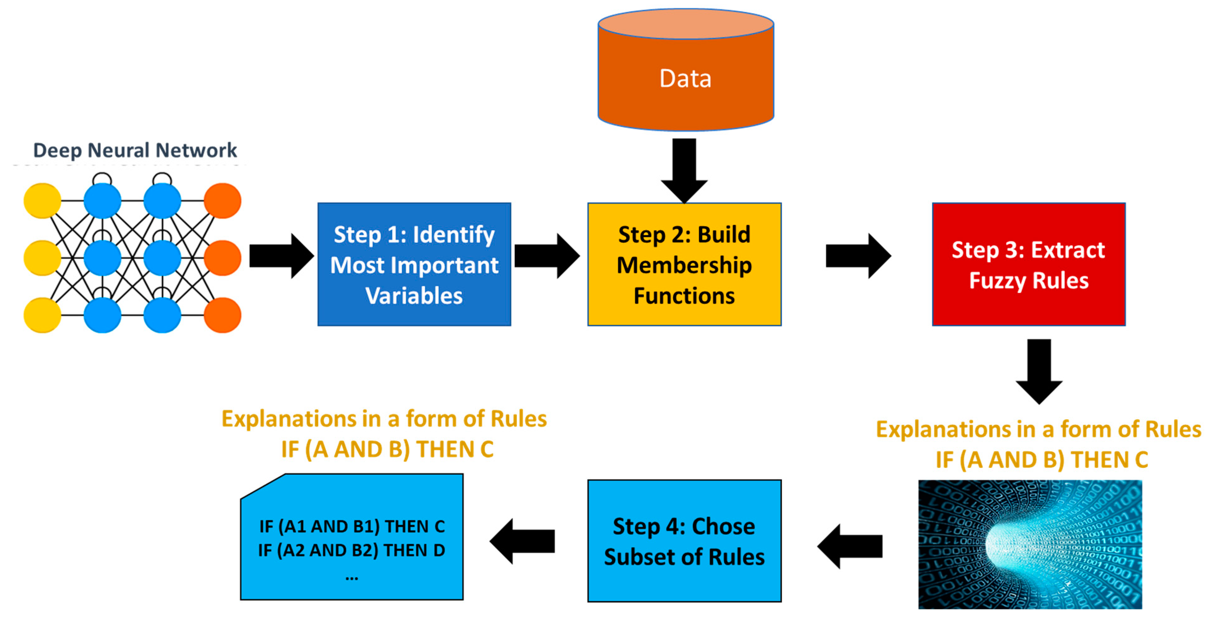
3. Materials and Methods

The FuzRED method seeks to deliver a set of rules that provide an accurate, human-understandable picture of broad model behavior. Importantly, this method provides users with the flexibility to restrict or expand the desired level of granularity at which the rulesets are generated and optimized. This flexibility is described later in Section 3.1 and Section 3.2.

The main steps of the explainability method that we developed are shown in Figure 1. We start with an AI model (e.g., shallow neural network, deep neural network, support vector machine, deep reinforcement learning network) that was trained to provide a decision or a prediction. For the ease of description, let us assume that the decision is a classification into one of n classes, but in reality, the decision/prediction could be of a different type. The first step is to determine from the large number of input features (sometimes thousands of them) the top k features that are the most important. In the second step, for each of the k features, a set of FMFs will be built. In the third step, fuzzy rules will be extracted for those features and the corresponding membership functions. These fuzzy rules are the explanations of why a given instance is classified into a given class (as such, they are local explanations). The full set of rules is a global explanation, explaining the behavior of the AI model. Often the full set of rules is not necessary, and a small subset of rules can be chosen that explains the model behavior. The fourth step of FuzRED is to choose that small subset of rules that explain the behavior of the AI model.

Figure 1. FuzRED approach.

3.1. Determination of the Most Important Features

The first step in the FuzRED method is to determine the most important features that contribute to model prediction. The goal of this step is to identify a set of model input features that will be the most useful antecedents to consider when generating the ruleset (e.g., the x in an IF x → THEN y rule). This step is important for two reasons: scale and comprehensibility. In terms of scale, the number of input features present in a given dataset (or used as input by a given AI model) can vary widely, with some datasets providing thousands of features for each sample. If the input feature space is sufficiently large, and all features are equally considered as possible antecedents, the computational load when generating our ruleset can rapidly become untenable. Furthermore, an overly large set of different antecedents within a resulting ruleset can easily be mentally overwhelming for humans who attempt to use the ruleset to understand model behavior. This is why identifying the top n most-influential input features enables comprehensibility as well as managing scale. The user has the flexibility to choose any number of the most influential input features that fit their needs.

In our method, we use SHAP values to identify a small set of features that are the most important to the model being explained (i.e., the features that have the largest impact on the predictions that the model makes). Lundberg and Lee [10] demonstrated that SHAP values were more consistent with human intuition than other explanation methods, and SHAP values have the advantage of providing a high degree of per-prediction precision when quantifying the input contributions of a single feature. Each SHAP value represents the contribution of a single feature value to a given model prediction, where positive SHAP values indicate features that increase the model prediction for a given example, and negative SHAP values indicate features that decrease the model prediction for a given example.

As previously mentioned, SHAP values are localized to a single example, making them poor candidates on their own for extrapolating global model behavior. However, a useful characteristic of SHAP is that the global importance of each feature can be derived by aggregating SHAP values across all the given examples in a dataset. The authors in [10] propose creating a global feature importance plot by calculating the mean absolute SHAP value for each feature across a dataset. In FuzRED, we leverage this metric (i.e., mean absolute value, which we term mean magnitude) and investigate additional candidate metrics for capturing global feature importance. These metrics provide different ways to aggregate feature contributions across all predictions, enabling a deeper analysis of feature importance. Specifically, we evaluated metrics such as frequency, mean contribution, mean magnitude, maximum contribution, maximum magnitude, and minimum contribution. Frequency measures how often a feature appears among the top n important features for a set of predictions, while mean contribution sums the signed (positive and negative) contributions of a feature for a set of predictions and divides them by the number of features. Mean magnitude aggregates the absolute values of these contributions and divides them by the number of features (it is the same as mean absolute SHAP used by others). The remaining metrics are derived by applying statistical operations (maximum, minimum) to the signed contributions and the maximum operation to the magnitude. Despite its name, the minimum contribution does not find the least important features (we would not be interested in those); because some of the SHAP values are negative, the minimum contribution finds the features for which the contributions are the most negative (these are large contributions, just in the negative direction). These six metrics are then compared to identify the most informative features and are used to select the top n candidates as the antecedents available for use during rule generation.

The above step presents the first instance of the granular flexibility mentioned at the beginning of Section 3. As previously referenced by Molnar, humans have limited capacity for holding large volumes of data in their short-term memory. In this step, n can be chosen to suit the needs of the chosen dataset, model, and analyst. For some cases, excessively large datasets might warrant a higher n value in order to provide a detailed, granular analysis of the impact the large feature space has on the resulting model predictions. In other cases, an easy-to-comprehend list of rules based on a small subset of features might be preferable for building trust among subject matter experts (SMEs).

We often choose a value of 20 for n to provide a balance between a sufficiently small feature space and an acceptable level of analysis of the resulting ruleset for benchmarking purposes. Ideally, n should be chosen after a careful analysis of the balance among the density of high-impact features across the dataset, the available computational resources, and the potential for cognitive overwhelm on human analysts from the resulting ruleset.

3.2. Building FMFs

After identifying the top n features, in the second step of FuzRED, we create FMFs for each feature by fitting Gaussian mixture models (GMMs) to the values observed in the training set. GMM [25] is a soft clustering machine learning method used to determine the probability that each data point belongs to a given cluster (it produces fuzzy clusters). The data point can belong to several clusters, each with a different probability, and those probabilities sum to 1. A Gaussian mixture is composed of several Gaussians, each identified by k ∈ {1, …, K}, where K is the number of clusters of our data set. When we require m membership functions per feature, we set K to m (i.e., if we want 2 membership functions, K is set to 2). The user can require a different number of FMFs for different features. This is the second flexible element of FuzRED: the user can choose as many or as few FMFs per feature as desired.

Given that GMMs perform soft clustering, they can be used to automatically learn FMFs from the data. Those FMFs will have a Gaussian shape. This allows the user to skip the process of manually defining all the FMFs for all the features, but instead rely on an automatic method.

GMMs are generated separately for each of the top n features. We wrote software that allows obtaining any number of membership functions for a feature the user desires. We often use two or three membership functions per feature: this is often sufficient and leads to a lower number of rules than using more membership functions. However, the method we developed is general and produces any desired number of FMFs per feature.

If the user desires three membership functions per feature, K is set to 3, and each mixture model consists of three components, corresponding to three fuzzy classes—e.g., low, medium, and high. These FMFs are then applied to both the training and test datasets to generate fuzzy membership data for 3 × n fuzzy classes (three per feature).

Then, we perform rule extraction using the FARM method described in Section 3.3 to automatically extract fuzzy association rules from the test data.

3.3. Extracting Fuzzy Association Rules

FuzRED’s third step is the automatic extraction of fuzzy association rules from the test data. Uncovering hidden and previously unknown patterns and insights from data is usually the primary objective of data mining. When these insights are expressed as relationships among different attributes, the process is referred to as association rule mining (ARM). Introduced by Agrawal et al. [22], ARM was originally developed to identify interesting co-occurrences within supermarket data, a classic problem known as market basket analysis. ARM identifies frequent itemsets (i.e., combinations of items that are purchased together in at least N transactions in the database) and then generates association rules based on these itemsets. For example, if {X, Y} is a frequent itemset, ARM can generate rules such as X → Y or Y → X. A simple association rule in the context of consumer behavior might be:

IF (Bread AND Butter) THEN Milk

This rule indicates that if a customer purchases bread and butter, they are also likely to purchase milk. Such rules can be highly valuable for store managers in determining how to organize products on shelves to maximize sales. While some rules, like the example above, may seem intuitive, ARM is particularly powerful because it can also reveal hidden patterns that may not be immediately obvious to SMEs. One famous example is the surprising rule:

IF (Diapers) THEN Beer

Initially, store managers were skeptical of this finding, suspecting a flaw in the ARM methodology. However, upon closer examination of the transaction data, they found that this pattern was indeed prominent, particularly in the evenings. The explanation was that dads were often asked to pick up diapers on their way home from work and, while doing so, rewarded themselves by purchasing beer. This insight, which would not have been obvious without ARM, demonstrates the method’s ability to reveal non-trivial, actionable knowledge.

Fuzzy association rules [23] extend the concept of association rules by introducing the ability to handle continuous or categorical variables with a degree of uncertainty. These rules take the following form:

IF (X IS A) THEN (Y IS B)

where X and Y are variables, and A and B are fuzzy sets that characterize X and Y respectively. A simple example of fuzzy association rule for a medical application is the following:

• IF (Temperature IS Strong Fever) AND (Skin IS Yellowish) AND (Loss of appetite IS Profound) THEN (Hepatitis is Acute)
• The rule states that a patient exhibiting a strong fever, yellowish skin, and a profound loss of appetite is likely suffering from acute hepatitis. “Strong Fever”, “Yellowish”, “Profound”, and “Acute” are membership functions of the variables Temperature, Skin, Loss of appetite, and Hepatitis, respectively. To illustrate this, consider the FMFs for the variable Temperature given in Figure 2. According to the definition in that figure, a person with a body temperature of 100 °F has a “Normal” temperature with a membership value of 0.2 and, simultaneously, has a “Fever” with a membership value of 0.78. These FMFs provide a nuanced way to interpret data, reflecting the complexity of real-world situations. More information on fuzzy logic and fuzzy membership functions can be found in [11].
  

  Figure 2. FMFs for the fuzzy feature Temperature: Low, Normal, Fever, Strong Fever, and Hyperthermia.

More formally, let D = {t₁, t₂, …, t_n} represent the transaction database, where each t_i is a transaction in D. Let I = {i₁, i₂, …, i_m} be the universe of items. A set X⊆I of items is called an itemset. When X has k elements, it is called a k-itemset. An association rule is an implication of the form X → Y, where X⊂I, Y⊂I, and X∩Y = ∅.

ARM and FARM rules have certain metrics associated with them. The three metrics that we use for evaluation and comparison of our method are support, confidence, and coverage. The support of an itemset, X, is defined as follows:

$$Support\left(X\right)={\displaystyle \frac{number records with X}{ number records in D}}={\displaystyle \frac{n_x}{n}}=p_x$$

(3)

where n is the number of records in D, n_x is the number of records with X, and p_x is the associated probability. The support of a rule (X → Y) is defined as follows:

$$Support\left(X\to Y\right)={\displaystyle \frac{number of records with X and Y}{number of records in D}}={\displaystyle \frac{n_{xy}}{n}}=p_{xy}$$

(4)

where n_xy is the number of records with X and Y and p_xy is the associated probability.

We can also define the concept of fuzzy support. In order to do this, we first need to define how we determine whether (and to what degree) one fuzzy set is a subset of another. To this end, we define the matching degree (MD) of one set, $S_1$, to another, $S_2$, as follows:

$${MD}_{S_1}\left(S_2\right)=\underset{f_i\in F_1}{\mathit{min}}{f}_i\left(S_2\right)$$

(5)

where $F_1$ is the set of membership functions inherently selected by $S_1$. We note that the min function in this definition is a T-norm. There are many other options for a T-norm that can be chosen, and a discussion of these goes beyond the scope of this paper, but for our purposes we always use the minimum function. We can now define the fuzzy support of a rule (X → Y) as follows:

$$Fuzzy Support \left(X\to Y\right)={\displaystyle \frac{sum of the MD of X and Y to records in D }{number of records in D}}={\displaystyle \frac{\sum _{r\in D}{MD}_{\left(X\to Y\right)}\left(r\right)}{n}}$$

(6)

The confidence of a rule (X → Y) is defined as follows:

$$Confidence \left(X\to Y\right)={\displaystyle \frac{number of records with X and Y}{number of records with X}}={\displaystyle \frac{n_{xy}}{n_x}}={\displaystyle \frac{n_{xy}}{n}}\times {\displaystyle \frac{n}{n_x}}={\displaystyle \frac{p_{xy}}{p_x}}$$

(7)

Similarly, the fuzzy confidence of a rule (X → Y) can be defined as follows:

$$Fuzzy Confidence \left(X\to Y\right)={\displaystyle \frac{sum of the MD of X and Y to records in D}{sum of the MD of X to records in D}}={\displaystyle \frac{\sum _{r\in D}{MD}_{\left(X\to Y\right)}\left(r\right)}{\sum _{r\in D}{MD}_X\left(r\right)}}$$

(8)

Confidence can be treated as the conditional probability (P(Y|X)) of a transaction containing X also containing Y. A high confidence value suggests a strong association rule. However, care must be taken in making this inference. For example, if the antecedent (X) and consequent (Y) both have a high support, the rule could have a relatively high confidence even if they were independent.

Support and confidence enable us to compare individual rules, but we also need to be able to compare sets of rules. An important metric for rule sets is coverage. This metric tries to capture how well a rule set “covers” a given data set, or what percentage of the records in the data set are in the support of one of the rules in the rule set. This concept is straightforward for crisp rules, but fuzzy rules introduce some complexities. We can define the coverage of a rule set, R, over a data set, D, as follows:

$${Coverage}_R\left(D\right)={\displaystyle \frac{number of records with X and Y for some X\to Y in R}{number of records in D}}={\displaystyle \frac{ \left|{\bigcup }_{X\to Y \in R}\left\{d\in D \right|X\cup Y\subset d\}\right|}{n}}$$

(9)

It is often the case that the MD of a fuzzy rule to a data record is non-zero but extremely small. Thus, including all records with non-zero MD for some rule in a fuzzy rule set does not provide an accurate view of the coverage of that rule set. Therefore, we need to set a threshold which we call minCov for the minimum MD needed for a data record to be counted as “covered”. We also need to define the maximum matching degree (MMD) of a rule set. This is a generalization of the MD defined above for individual rules. The MMD of a rule set, R, on a data record, r, can be defined as follows:

$${MMD}_R \left(r\right)=\underset{X\to Y\in R}{\mathit{max}}{MD}_{X\to Y}\left(r\right)$$

(10)

We can now define the fuzzy coverage of a rule set, R, over a data set, D, as follows:

$$\begin{array}{l}{Fuzzy Coverage}_R \left(D\right)={\displaystyle \frac{number records with MD>minCov for some rule in R}{number records in D}}\\ \hspace{1em}\hspace{1em}\hspace{1em}\hspace{1em}\hspace{1em}\hspace{1em}\hspace{1em}\hspace{1em}={\displaystyle \frac{\left|\left\{d\in D|{MMD}_R\left(d\right)\ge min\_Cov\right\}\right|}{n}}\end{array}$$

(11)

When executing FuzRED, we set the minimum support threshold for the rules to 0.001, although a higher or lower support can be used. When selecting the number of antecedents that are available for a single rule, we often set the maximum number to three. Humans have difficulty quickly understanding rules with a large number of antecedents; therefore, for most applications, we discourage using a larger number.

3.4. Choosing a Subset of Rules

Although FARM typically generates thousands of rules, only a subset is relevant for interpretability. Humans do not like looking at such a large number of rules and would rather have a much smaller subset summarizing what the network does. We use the following method for pruning the rule set to find an optimal minimum set of rules. For each of the six methods for determining the most important features, we order the rules first by decreasing confidence, and then by decreasing support. Then we take the first rule from the ordered set of rules and determine for which examples from the test set the rule applies. We remove the examples to which it applies from the test set. Then, we take the next rule from the rule set and repeat the process. We continue the process until there are no more examples in the test set or no more rules.

4. Results

We applied the FuzRED method to three AI models, each trained for a different learning task with a different dataset. Two models were feed-forward deep neural networks performing binary classification tasks (spam email identification and phishing link detection, respectively). The third model was a DRL model trained to perform a benchmark robotics task. In the sections below, we present results for our FuzRED method, and results generated using the existing Anchors method.

4.1. Spam Email Identification

The SPAM Email Database [26], available from the University of California Irvine (UCI) Machine Learning Repository, was utilized for this study. This dataset contains spam emails identified as such by the recipients or the email postmaster. The non-spam emails consist of both work and personal emails identified as non-spam by the recipients. The dataset was submitted to the UCI Machine Learning Repository in July 1999. The dataset comprises 4601 total instances, 1813 of which are labeled as spam. There are 57 continuous data attributes, and the nominal class label is provided for each instance. Attributes include frequencies of select words and characters, as well as the statistics of uninterrupted sequences of capital letters in the emails. There are no missing attributes in this dataset. We do not have access to the text of the emails but only to frequencies of all the attributes in the emails. For more details on the attributes and their statistics, the reader is referred to [26].

To evaluate our explanation method, we trained a deep neural network model to make predictions on this dataset. The model consists of three fully connected hidden layers, each with 12 nodes using the rectified linear unit (ReLU) activation function, followed by a final fully connected layer with a single node utilizing the sigmoid activation function. We randomly selected 70% of the SPAM email dataset to serve as the training set. All input data were normalized using a StandardScaler object [27] before being fed into the model, and the resulting model achieved 89% accuracy on the test set.

4.1.1. FuzRED Results

We employed six methods for determining the most important features: mean magnitude, frequency, mean contribution, maximum contribution, maximum magnitude, and minimum contribution. These methods are described in Section 3.1.

SHAP can be used for both local and global explanations. Usually, for global explanations, the absolute Shapley values of all instances in the data are averaged. Passing a matrix of SHAP values to the bar plot function [28] creates a global feature importance plot, where the global importance of each feature is taken to be the mean absolute SHAP value for that feature over all the given samples. Figure 3 shows the plot created using the bar plot function with the top 20 features. Figure 4, Figure 5, Figure 6, Figure 7 and Figure 8 show the bar plots we created for the remaining five methods.

Figure 3. Spam dataset: bar plot for the top 20 features determined using the mean magnitude method.

Figure 4. Spam dataset: bar plot for the top 20 features determined using the frequency method.

Figure 5. Spam dataset: bar plot for the top 20 features determined using the mean contribution method.

Figure 6. Spam dataset: bar plot for the top 20 features determined using the maximum contribution method.

Figure 7. Spam dataset: bar plot for the top 20 features determined using the maximum magnitude method.

Figure 8. Spam dataset: bar plot for the top 20 features determined using the minimum method.

All the features determined to be the most important by frequency and maximum magnitude methods are shared by at least one other method. Mean contribution and mean magnitude methods each have one feature that was not determined to be the most important by any other methods (word_freq_conference and word_freq_85); maximum contribution has three features in the top 20 not identified by any of the other five methods: word_freq_report, word_freq_money, and word_freq_parts. Minimum contribution has the largest number of features not identified as the most important by any other method: word_freq_telnet, word_freq_857, word_freq_table, word_freq_technology, char_freq, and capital_run_length_longest.

Figure 9 and Figure 10 show the FMFs for word_freq_george and word_freq_hp. Figure A1, Figure A2 and Figure A3 in Appendix A.1 show the FMFs for word_freq_meeting, char_freq_$, and char_freq_!. These are some of the features that were determined to be the most important by at least one of the methods and that are used in the rule explanations in the next section.

Figure 9. Spam dataset: FMFs for word_freq_george, i.e., low, medium, and high, are shown in red, green, and blue, respectively.

Figure 10. Spam dataset: FMFs for word_freq_hp, i.e., low, medium, and high are shown in red, green, and blue, respectively.

Word_freq_george describes the frequency of the word george (how many times it appeared) in an email. Figure 9 shows the FMFs for word_freq_george: low, medium, and high. In the spam dataset, the largest frequency of george is 33. FMF low has a value of 1 for word_freq_george values from 0 to 2.223. For values larger than 2.223 but smaller than 12.557, the value of FMF medium is 1.0. Values larger than or equal to 12.557 but smaller than 13.433, belong to two FMFs: medium and high. For example, for 13.0, the value of FMF medium is 0.474 and that of MFM high is 0.526. This means that, when word_freq_george is 13.0, it is both medium and high (to the degree defined by the value of the appropriate FMF). For values larger than 13.433, the value of FMF high is 1. FMFs are continuous; however, when the feature itself is an integer (frequency is always an integer number), the above description can be rewritten as follows. FMF low has a value of 1 for word_freq_george values from 0 to 2. For values between 3 and 12, the value of FMF medium is 1.0. The value 13 belongs to two FMFs: medium and high. Starting at 14, the value of FMF high is 1.

Word_freq_hp describes the frequency of the word hp in an email. Figure 10 shows the three FMFs for word_freq_hp. In the spam dataset, the largest frequency of hp is 21. This is also an integer variable and its FMFs can be described as follows. FMF low has a value of 1 for the word_freq_hp value of 0. For values between 1 and 7, the value of FMF Medium is 1.0. A value of 8 belongs to two FMFs: medium and high. Starting at 9, the value of FMF high is 1.

Figures in Appendix A.1 (A1–A3) show the three FMFs for word_freq_000, word_freq_meeting, and char_freq_$, respectively. Word_freq_000 describes the frequency of 000 in an email. Word_freq_meeting describes the frequency of the word meeting in an email. Char_freq_$ describes the frequency of the character $ in an email.

When running fuzzy association rule mining, we limited the number of antecedents to three, we set the minimum confidence (Equation (8)) of a rule to 0.6, and the minimum support (Equation (6)) to 0.001. Most of the rules found by FuzRED are easy to understand. As an example, below we show some of the rules extracted using the maximum magnitude choice of features.

• IF (word_freq_george IS High) THEN No-Spam, sup = 0.0263, conf = 1

This rule says that if the frequency of the word george is high (see Figure 3), then the email is no-spam with a confidence value of 1 (the rule is always true). This rule has a support of 2.63%, which means that it explains 2.63% of the dataset. At the beginning, this rule seems to be a little surprising; however, when we assessed the description of the dataset, we noticed that it said the no-spam rules were provided from personal and business emails of the dataset creators, and one of them was George Forman. In view of this information, the rule makes perfect sense.

• IF (word_freq_hp IS Medium) THEN No-Spam, sup = 0.0753, conf = 1
• The above rule says that if the frequency of the word hp (Hewlett Packard) is medium (see Figure 10), then the email is no-spam. The support of the rule is 7.53% and the rule is always true. The creators of the dataset were all HP employees, and many no-spam emails provided included their business emails, so this rule also makes perfect sense. A similar rule is shown below:
• IF (word_freq_hp IS High) THEN No-Spam, sup = 0.0145, conf = 1
• Some no-spam rules are related to the frequency of the words meeting, 1999, or lab:
• IF (word_freq_meeting IS Medium) THEN No-Spam, sup = 0.0217, conf = 1
• IF (word_freq_meeting IS High) THEN No-Spam, sup = 0.0046, conf = 1
• IF (word_freq_george IS Medium AND word_freq_1999 IS Medium) THEN No-Spam, sup = 0.0014, conf = 1

This dataset was donated on 6/30/1999; it is very possible that the no-spam emails were chosen mostly from the beginning of 1999.

The spam rules often use the character frequency of $ or !:

• IF (char_freq_$ IS High) THEN Spam, sup = 0.0033, conf = 1
• IF (char_freq_$ IS Medium AND char_freq_! IS Medium) THEN Spam, sup = 0.0028, conf = 1

Since spam emails are often about becoming rich (receiving $), and some use a lot of exclamation points, the above rules are sensible.

• IF (capital_run_length_average IS Medium) THEN Spam, sup = 0.0026, conf = 1
• The above rule says that if the average length of uninterrupted sequences of capital letters is Medium, then the email is always spam.
• IF (char_freq_$ IS Medium AND capital_run_length_total IS High) THEN Spam, sup = 0.0020, conf = 1
• The above rule says that if the total number of capital letters in the email is high, then the email is always spam. Historically, spam emails use a lot of capital letters, so this rule is logical.

Additional FuzRED rules for spam email identification are shown in Appendix A.1.

Depending on which of the six methods is being used for determining the most important features and the minimum confidence of the rules (0.6 to 1), FuzRED extracts a different number of rules. The results are shown in Table 1. The table is arranged in descending order by total coverage (Equation (11)) and then in ascending order by the number of rules after pruning. The total coverage of this set of rules ranges from 0.9717 to only 0.1554.

Table 1. Spam: number of rules extracted by FuzRED for different methods of determining the most important features.

Row Number	Min Rule Confidence	Method	Number of Rules	Number of Rules After Pruning	Total Coverage
1	0.6	Maximum contribution	609	139	0.9717
2	0.6	Mean magnitude	545	128	0.9671
3	0.6	Frequency	578	133	0.9671
4	0.7	Mean magnitude	387	126	0.9414
5	0.7	Frequency	384	131	0.9414
6	0.7	Maximum contribution	353	135	0.9309
7	0.6	Mean contribution	406	109	0.9289
8	0.6	Maximum magnitude	342	96	0.9243
9	0.7	Mean contribution	230	106	0.9019
10	0.7	Maximum magnitude	238	90	0.8907
11	0.6	Minimum contribution	195	67	0.7966
12	0.8	Mean magnitude	253	114	0.6458
13	0.8	Frequency	250	118	0.6248
14	0.8	Mean contribution	182	102	0.6004
15	0.9	Mean magnitude	204	102	0.5747
16	0.9	Frequency	209	107	0.5583
17	0.95	Mean magnitude	158	94	0.5332
18	0.7	Minimum contribution	179	62	0.5346
19	0.95	Frequency	161	99	0.5168
20	0.96	Mean magnitude	149	91	0.5122
21	0.9	Mean contribution	144	92	0.5089
22	0.97	Mean magnitude	139	87	0.5010
23	0.96	Frequency	154	96	0.4924
24	0.8	Maximum magnitude	157	81	0.4852
25	0.98	Mean magnitude	138	85	0.4918
26	0.97	Frequency	146	91	0.4852
27	0.95	Mean contribution	125	87	0.4885
28	0.98	Frequency	144	89	0.4760
29	0.96	Mean contribution	116	83	0.4635
30	0.99	Mean magnitude	121	76	0.4602
31	0.99	Frequency	126	80	0.4523
32	0.97	Mean contribution	113	80	0.4523
33	0.98	Mean contribution	111	77	0.4457
34	0.9	Maximum magnitude	120	71	0.4332
35	0.99	Mean contribution	100	70	0.4134
36	0.8	Maximum contribution	212	120	0.3568
37	0.95	Maximum magnitude	99	66	0.4009
38	0.8	Minimum contribution	104	56	0.4075
39	0.96	Maximum magnitude	93	63	0.3726
40	0.97	Maximum magnitude	87	60	0.3568
41	0.98	Maximum magnitude	88	59	0.3562
42	0.9	Minimum contribution	86	49	0.3805
43	0.99	Maximum magnitude	82	56	0.3430
44	0.9	Maximum contribution	183	108	0.2877
45	1	Mean magnitude	72	48	0.3364
46	0.95	Minimum contribution	71	46	0.3476
47	0.96	Minimum contribution	68	46	0.3476
48	1	Frequency	73	47	0.3246
49	0.95	Maximum contribution	161	101	0.2646
50	1	Mean contribution	64	46	0.3160
51	0.96	Maximum contribution	158	99	0.2600
52	0.97	Maximum contribution	151	94	0.2535
53	0.98	Maximum contribution	148	91	0.2508
54	0.97	Minimum contribution	64	43	0.3226
55	0.99	Maximum contribution	136	87	0.2357
56	0.99	Minimum contribution	60	40	0.3061
57	0.98	Minimum contribution	60	40	0.3061
58	1	Maximum magnitude	54	35	0.2791
59	1	Minimum contribution	60	36	0.2791
60	1	Maximum contribution	77	49	0.1554

When explaining the decisions of a neural network, one may wish to minimize the number of rules while still achieving the required level of dataset coverage. For example, if a coverage of at least 0.9 is desired, Table 1 shows that nine methods meet this criterion. Among them, the best option in terms of rule count is method 8 (maximum magnitude, minimum rule confidence of 0.6), which achieves a coverage of 0.9243 with just 96 rules after pruning. If a smaller ruleset is desired and a lower coverage threshold, such as 0.75, is acceptable, then method 11 (minimum contribution, minimum rule confidence of 0.6) provides a ruleset with just 67 rules. These 67 rules are listed in Appendix A.1, in Table A1. For cases where covering just over half of the dataset is sufficient, method 18 (minimum contribution, minimum rule confidence of 0.7) reduces the ruleset further to 62 rules. Thus, the optimal method depends on the specific balance between coverage requirements and the desire to minimize ruleset complexity for a given application.

4.1.2. Anchors Results

In order to evaluate and compare Anchors rules with those from FuzRED, we wrote a script to use the Anchors library to explain the exact same trained model and set of data. The script used anchor_tabular.AnchorTabularExplainer to generate the anchors and wrapped the model for compatibility with the Anchors framework. We wrote a fit_anchor function in order to compute the actual precision (Equation (1)) and coverage (Equation (2)) metrics for the anchor rules. This function parses the body of the rule and converts it to the equivalent logical conditions and then applies it to the full set of test data to find all instances to which the anchor applies. For this to work properly, we needed to round all of the feature data to two decimal places, as the values in the Anchors were rounded. Lastly, the function computes and returns the computed coverage and precision metrics for the anchors.

When Anchors was executed to obtain rules with a maximum of three antecedents, it produced 1520 rules. Some of the rules were repeating themselves and, therefore, we developed software to remove repeating rules and ended up with 648 distinct rules. Most rules have three antecedents, some have two, and a handful have just one. The rules have a precision ranging from 1 to 0.5312 and a coverage ranging from 0.5872 to 0.0007.

Below are some example rules. The rule with the highest coverage is the following:

• IF (char_freq_$ <= 0.05 AND word_freq_free <= 0.00 AND word_freq_money <= 0.00) THEN No-Spam, coverage = 0.5872, precision = 0.8543
• This rule says that if the frequency of $ is less than or equal to 0.05, and the frequencies of free and money are less than or equal to 0, then the email is No-Spam in 85.43% of the cases. Of course, frequency cannot be a negative number, and frequency is an integer; therefore, being less than or equal to 0.05, is the same as being zero. Therefore, the rule actually says that if the frequency of $, free, and money is zero, then the email is No-Spam in 85.43% of the cases. The 0.05 threshold in the rule is arbitrary. The rule has a large coverage (58.72%) and is true in 85.43% cases.
• IF (word_freq_hp > 0.00 AND char_freq_! <= 0.00 AND word_freq_remove <= 0.00) THEN No-Spam, coverage = 0.1672, precision = 1
• This rule says that if the frequency of hp is greater than 0 and the frequencies of ! and remove are less than or equal to 0, then the email is always No-Spam. Of course, frequency cannot be a negative number, so the rule actually says that if the frequency of hp is greater than 0 and the frequencies of ! and remove are 0, then the email is always No-Spam. This rule covers 16.72% of the data.

The rules above are relatively easy to understand, as they use zero as the threshold. However, most rules use very different numbers as the threshold. These numbers might seem arbitrary to the person who wants to understand the decisions the network is making.

• IF (word_freq_remove > 0.00 AND char_freq_$ > 0.05 AND capital_run_length_longest > 43.00) THEN Spam, coverage = 0.0671, precision = 1
• IF (word_freq_remove > 0.00 AND char_freq_$ > 0.05 AND capital_run_length_average > 3.71) THEN Spam, coverage = 0.0579, precision = 1
• IF (word_freq_3d > 0.00 AND capital_run_length_average > 3.71 AND word_freq_you > 2.63) THEN Spam, coverage = 0.0007, precision = 1

All the features in the three rules above are integer; therefore, the thresholds used (i.e., 0.05, 3.71, 2.63) are very arbitrary and confusing.

Additional Anchors rules for the Spam email identification are shown in Appendix A.1.

4.2. Phishing Link Detection

This study leveraged the phishing link detection dataset curated by Hannousse and Yahiouche [29]. This dataset has 11,430 samples, each containing 87 features extracted from each URL. Fifty-six features were extracted by analyzing the text of the URL (URL-based), 24 features were extracted by analyzing the content of the website hosted at the URL (content-based), and seven features were extracted by gathering external information about the URL (external-based). Examples of URL-based features include the presence of common terms in the URL (such as ‘www’ or ‘.com’) or the ratio of digits to other characters in the URL. Content-based feature examples include the presence of invisible iframe objects on the site or an empty HTML <title> tag. External-based feature examples include whether or not the URL is from a WHOIS-registered domain, or the number of visitors to the site. In total, this dataset contains 87 features that are a combination of integer, floating point, and binary values. The authors in [29] provide a full description of the features alongside details regarding dataset collection methods.

The dataset was first split into 7658 training samples, while 3772 samples were reserved for testing. A deep feed-forward neural network was constructed with three hidden layers. The model was trained for 200 epochs with a batch size of 256. All input data were normalized using a StandardScaler object [27] before being fed into the model, and the resulting model achieved 85% accuracy on test data.

4.2.1. FuzRED Results

We employed six methods for determining the most important features: frequency, mean contribution, mean magnitude, maximum contribution, maximum magnitude, and minimum contribution. Figure 11, Figure 12, Figure 13, Figure 14, Figure 15 and Figure 16 show the 20 most important features for mean magnitude, frequency, mean contribution, maximum contribution, maximum magnitude, and minimum contribution, respectively. All the features determined as being the most important by frequency and maximum magnitude methods are shared by at least one other method. Maximum contribution has one feature that was not determined as the most important by any other method (iframe); mean magnitude has two such features (nb_slash, ratio_extMedia), and mean contribution has three features not determined as being the most important by any other method (dns_record, ratio_intHyperlinks, web_traffic). Minimum contribution has the largest number of features (11) not identified as being the most important by any other method: length_words_raw, nb_percent, avg_word_host, longest_word_host, length_url, whois_registered_domain, abnormal_subdomain, domain_in_brand, nb_dslash, onmouseover, and popup_window.

Figure 11. Phishing dataset: bar plot for the top 20 features determined using the mean magnitude method.

Figure 12. Phishing dataset: bar plot for the top 20 features determined using the frequency method.

Figure 13. Phishing dataset: bar plot for the top 20 features determined using the mean contribution method.

Figure 14. Phishing dataset: bar plot for the top 20 features determined using the maximum contribution method.

Figure 15. Phishing dataset: bar plot for the top 20 features determined using the maximum magnitude method.

Figure 16. Phishing dataset: bar plot for the top 20 features determined using the minimum contribution method.

For each feature, we used Gaussian mixture models to construct two membership functions (low and high). Figure 17 and Figure 18 show the membership functions for the features: length_words_raw and ratio_intMedia. The FMFs for features, nb_dots, and nb_www are shown in Appendix A.2. These features are used in the example rules described in the FuzRED Rules section, Section 4.2.1. The feature descriptions in this section are taken from [30].

Figure 17. Phishing dataset: FMFs for length_words_raw. Low and high are shown in red and blue, respectively.

Figure 18. Phishing dataset: FMFs for ratio_intMedia. Low and high are shown in red and blue, respectively.

Length_words_raw describes the number of words in a URL. In the phishing dataset, the largest length_words_raw is 106 (Figure 17 shows the FMFs). FMF low has a value of 1 for length_words_raw values from 1 to 28.240; for 32.000, the FMF low has a 0.299 value, and FMF high has a 0.701 value. This means that when length_words_raw is 32.000, it is both low and high (to the degree defined by the value of the appropriate FMF). Starting at 35.023, the value of FMF high is 1.

Legitimate websites mostly use media (images, audio, and video) stored in the same domain. Phishing websites use more external media, usually stored in the target website domain, to save storage space. Ratio_intMedia estimates the ratio of internal media file links and uses it for distinguishing legitimate from phishing websites. In the phishing dataset, the largest ratio_intMedia is 100 (Figure 18 shows the FMFs). FMF low has a value of 1 for ratio_intMedia values from 0 to 38.804; for 49.155, the FMF low has a value of 0.501, and FMF high has a 0.499 value. This means that when ratio_intMedia is 49.155, it is both low and high (to the degree defined by the value of the appropriate FMF). Starting at 59.516, the value of FMF High is 1.

The FMFs for nb_dots and nb_www are shown in Appendix A.2.

When running fuzzy association rule mining, we limited the number of antecedents to three, we set the minimum confidence (Equation (8)) to 0.6, and we set the minimum support (Equation (6)) to 0.001. Most of the rules found by FuzRED are easy to understand. As an example, below we show some of the rules extracted using the maximum magnitude choice of top features.

• IF (nb_dots IS High) THEN Phishing, sup = 0.0039, conf = 1This rule says that if the nb_dots (number of dots in the URL) is high, then the URL is always predicted to be a phishing domain by the model. An example of such a URL is below (13 dots in the domain name):
• http://https.email.office.nhc8fso9liwz2e1rk12vhqaxgeq4g.hgbtmd8eshlu1rkesgz11.tk0mqbhgkkuvsf3u821.1sytn1idkv8s2qm4ehh7jja7d.mne8jnxrh8klahtqu.0fll4ryeb76852jeplwk9ckd6zqof.2wvxm5n6uamkxq7wxhpbxaq1a4.cxdtens.duckdns.org/365NewOfficeG15/jsmith@imaphost.com/paul/
• IF (nb_www IS High AND length_words_raw IS High) THEN Phishing, sup = 0.0023522, conf = 1.0
• Length_words_raw is an integer that refers to how many words there are in a URL. The rule says that if the nb_www and length_words_raw are high, then the URL is a phishing one. In the phishing URL below, nb_www is 2, and length_words_raw is 16:
• http://timetravel.mementoweb.org/reconstruct/20141123205914mp_/https:/www.paypal.com/signin?returnuri=https:/www.paypal.com/cgi-bin/webscr?cmd=_account
• IF (page_rank IS High AND nb_hyperlinks IS High) THEN No-Phishing, sup = 0.0141772, conf = 0.9991)

Page_rank is an algorithm used by Google Search to rank web pages in their search engine results. Phishing web pages are not very popular, hence, they are supposed to have low page ranks compared to legitimate web pages. Legitimate (No-Phishing) websites are supposed to consist of a larger number of pages compared with phishing ones. Therefore, the number of links in a URL contents (nb_hyperlinks) is considered for distinguishing phishing websites. The rule above says that if both the page_rank and nb_hyperlinks are high, then almost always (conf = 0.9991) the website is No-Phishing.

Depending on which of the six methods we are using for determining the most important features and the minimum confidence of the rules (0.6 to 1), FuzRED extracts a different number of rules. The results are shown in Table 2. The table is arranged in descending order by total coverage (Equation (11)) and then in ascending order by the number of rules after pruning. The total coverage of this set of rules ranges from 1.0 to only 0.0424.

Table 2. Phishing: number of rules extracted by FuzRED for different methods for determining the most important features.

Row Number	Min Rule Confidence	Method	Number of Rules	Num of Rules After Pruning	Total Coverage
1	0.6	Frequency	912	163	1
2	0.6	Mean magnitude	939	164	1
3	0.7	Mean magnitude	773	164	1
4	0.8	Mean magnitude	582	164	1
5	0.7	Frequency	765	162	0.9992
6	0.8	Frequency	588	159	0.9984
7	0.6	Minimum contribution	299	100	0.9981
8	0.6	Maximum contribution	113	56	0.9966
9	0.7	Minimum contribution	257	95	0.9960
10	0.6	Mean contribution	366	124	0.9952
11	0.9	Frequency	413	141	0.9862
12	0.7	Maximum contribution	100	53	0.9841
13	0.7	Mean contribution	294	115	0.9838
14	0.9	Mean magnitude	380	142	0.9825
15	0.6	Maximum magnitude	220	58	0.9793
16	0.8	Maximum contribution	69	52	0.9722
17	0.7	Maximum magnitude	187	56	0.9700
18	0.8	Minimum contribution	181	87	0.9669
19	0.95	Frequency	252	119	0.9517
20	0.95	Mean magnitude	238	118	0.9459
21	0.9	Minimum contribution	121	73	0.9427
22	0.96	Frequency	225	108	0.9337
23	0.96	Mean magnitude	210	106	0.9266
24	0.9	Maximum contribution	55	43	0.8834
25	0.95	Minimum contribution	95	61	0.7961
26	0.8	Mean contribution	195	89	0.7908
27	0.8	Maximum magnitude	116	48	0.7704
28	0.96	Minimum contribution	88	58	0.7216
29	0.97	Frequency	185	94	0.7235
30	0.97	Mean magnitude	175	91	0.6779
31	0.98	Frequency	139	75	0.6694
32	0.95	Maximum contribution	44	34	0.6622
33	0.96	Maximum contribution	49	32	0.6516
34	0.98	Mean magnitude	132	71	0.6259
35	0.99	Frequency	91	53	0.5623
36	0.99	Mean magnitude	90	54	0.5411
37	0.9	Mean contribution	103	58	0.5427
38	0.97	Minimum contribution	76	52	0.5005
39	0.9	Maximum magnitude	66	39	0.4907
40	0.95	Maximum magnitude	44	32	0.4801
41	0.96	Maximum magnitude	38	28	0.4629
42	0.98	Minimum contribution	65	47	0.4449
43	0.99	Minimum contribution	52	39	0.3624
44	0.97	Maximum contribution	33	25	0.2654
45	0.95	Mean contribution	62	40	0.2569
46	0.97	Maximum magnitude	38	26	0.2450
47	0.96	Mean contribution	58	38	0.2169
48	0.97	Mean contribution	54	38	0.2155
49	0.98	Maximum contribution	32	23	0.2121
50	0.98	Maximum magnitude	29	22	0.2092
51	0.99	Maximum contribution	22	16	0.1893
52	0.98	Mean contribution	45	35	0.1853
53	0.99	Mean contribution	29	27	0.1665
54	0.99	Maximum magnitude	23	17	0.1575
55	1	Frequency	23	16	0.0793
56	1	Mean magnitude	17	13	0.0745
57	1	Minimum contribution	20	15	0.0567
58	1	Maximum magnitude	15	10	0.0536
59	1	Mean contribution	11	9	0.0488
60	1	Maximum contribution	8	8	0.0424

When explaining the decisions of a neural network, one may wish to minimize the number of rules while still achieving a required level of dataset coverage. For example, if a coverage of at least 0.9 is desired, Table 3 shows that 23 methods meet this criterion. Among them, the best option in terms of rule count is method 16 (maximum contribution, minimum rule confidence of 0.8), which achieves a coverage of 0.9722 with just 52 rules after pruning. If a smaller ruleset is desired and a lower coverage threshold, such as 0.75, is acceptable, then method 27 (maximum magnitude, minimum rule confidence of 0.8) provides a ruleset with just 48 rules. These 48 rules are listed in Appendix A.2, Table A2. For cases where covering just over half of the dataset is sufficient, method 32 (maximum contribution, minimum rule confidence of 0.95) reduces the ruleset further to 34 rules.

Table 3. Hyperparameters used to train the PPO model.

Hyperparameter	Value
Discount factor (γ)	0.99
Entropy coefficient	0.05
Learning rate	0.0005
Batch size	1024
Number of layers	2
Layer size	128
Number of environments	16
Number of steps per update	2048

4.2.2. Anchors Results

When running Anchors, we requested rules with up to three antecedents. Anchors produced 3808 rules; once the repeating ones had been removed, we obtained 548 rules. Most of the rules have three antecedents, some have two, and a few have one. Some rules are easy to understand:

• IF (nb_star > 0.00) THEN Phishing, coverage = 0.0011, precision = 1
• Nb_star refers to the number of stars (*) in a URL. The above rule is always true and describes 0.11% of the dataset.

Most rules are much more difficult to understand.

• IF (page_rank <= 1.00 AND google_index > 0.00 AND longest_words_raw > 16.00) THEN Phishing, coverage = 0.1021, precision = 1
• Google_index is a binary variable describing whether a given domain is indexed by Google or not (1 means indexed, and 0 means not indexed); web pages not indexed by Google have a higher probability of phishing. The above rule says that if page_rank <= 1.00, the google_index > 0.00 (in reality google_index = 1, meaning indexed by google), and the longest_words_raw > 16.00, the web page is always phishing. It is unclear why URLs indexed by Google would be related to phishing; as such, this rule appears contradictory.
• IF (google_index <= 0.00 AND ratio_extErrors > 0.00 AND domain_registration_length > 446.75) THEN No-Phishing, coverage = 0.0684, precision = 0.9961
• The above rule is very difficult to comprehend: when google_index is 0, the page is not indexed by Google, so why would this be related to No-Phishing? In the dataset, ratio_extErrors is always > 0; therefore, this part of the rule does nothing. Finally, the domain_registration_length has a difficult-to-understand threshold value. The rule is true in 99.61% of cases.
• IF (google_index > 0.00 AND nb_hyperlinks <= 9.00 AND avg_words_raw > 8.00) THEN Phishing, coverage = 0.0551, precision = 0.9952

The rule above has difficult-to-understand thresholds.

Additional Anchors rules are shown in Appendix A.2.

4.3. Robotic Navigation

In this section, we demonstrate the application of the FuzRED explainability method to deep reinforcement learning (DRL) agents, expanding the scope of our explainability framework beyond traditional deep learning models. We created a toy model using the Miniworld package [30] and tasked an agent with vision-based navigation to achieve a sequence of objectives. We utilized a custom simulated environment in which an agent and three colored boxes—red, blue, and yellow—were placed in random positions. The agent’s goal was to reach each of the three boxes in a specified sequence: first the red box, then the blue box, and finally the yellow box. We used the Stable-Baselines3 package ver 2.3.2 [31] to train a proximal policy optimization (PPO) model to accomplish these objectives. To address the multi-goal navigation problem, we employed hierarchical reinforcement learning (HRL), which comprises a high-level policy for generating sub-goals and a low-level policy for executing actions. The high-level controller uses the current environmental observations to provide sub-goals to the low-level planner.

The agent processed the visual information it captured from the environment (shown in Figure 19) using an object detection model. Specifically, a pre-trained you look only once (YOLO) v8 [32] model was fine-tuned on screenshots from the Miniworld environment, which were manually labeled to detect the three colored boxes. YOLO provided reliable information about the position of each box by generating bounding box coordinates, which were then used as part of the state representation for the PPO agent. These coordinates included the x and y positions of each box’s center, as well as the height and width of each bounding box. The coordinates were normalized between 0 and 1 before being fed into the low-level planning agent. The final state space presented to the PPO model was a concatenated vector consisting of bounding box coordinates for the red, blue, and yellow boxes, combined with one-hot encoded vectors indicating the detection status of each box and which box was the current target. The agent had an action space consisting of turning right, turning left, moving forward, and moving backward.

Figure 19. Robotic navigation agent’s environment.

The training of the model involved using both step-based rewards and sub-goal completion rewards. The agent received a positive reward of 0.03 for each step it took that brought it closer to the target box, while moving away from the target resulted in a penalty of −0.03. When the agent successfully reached a sub-goal, it was rewarded with a value that increased based on how many sub-goals had already been completed and how efficiently the current sub-goal was achieved:

$$R_{sub-goal}=2\times nu{m}_{boxe{s}_{found}}\times \left(1-0.2\times {\displaystyle \frac{curren{t}_{step}}{\underset{\mathit{steps}}{\mathit{max}}}}\right)$$

(12)

This reward function incentivized the agent to find all boxes and do so as efficiently as possible, with a maximum of 1000 steps allowed per episode. The agent was trained using a vectorized environment, which allowed multiple versions of the environment to run simultaneously, thus speeding up the training process and providing diverse experiences for learning. During the training of the PPO model, we performed several rounds of hyperparameter tuning. The final hyperparameters selected are given in Table 3. The training process continued until the model performance converged, achieving all three sub-goals on average within 250 steps after approximately 700,000 training steps.

To generate rules explaining the model, we extracted features from the state space used to train the model, including bounding box coordinates, one-hot encoded detection statuses, and target indicators. These features are summarized in Table 4.

Table 4. Feature names and descriptions.

Feature Name	Description
red_box_position_x	The x coordinate of the center of the YOLO bounding box around the red box.
red_box_position_y	The y coordinate of the center of the YOLO bounding box around the red box.
red_box_width	The width of the YOLO bounding box around the red box.
red_box_height	The height of the YOLO bounding box around the red box.
blue_box_position_x	The x coordinate of the center of the YOLO bounding box around the blue box.
blue_box_position_y	The y coordinate of the center of the YOLO bounding box around the blue box.
blue_box_width	The width of the YOLO bounding box around the blue box.
blue_box_height	The height of the YOLO bounding box around the blue box.
yellow_box_position_x	The x coordinate of the center of the YOLO bounding box around the yellow box.
yellow_box_position_y	The y coordinate of the center of the YOLO bounding box around the yellow box.
yellow_box_width	The width of the YOLO bounding box around the yellow box.
yellow_box_height	The height of the YOLO bounding box around the yellow box.
red_box_detected	Binary feature that indicates if YOLO has detected the red box (0 = false, 1 = true).
blue_box_detected	Binary feature that indicates if YOLO has detected the blue box (0 = false, 1 = true).
yellow_box_detected	Binary feature that indicates if YOLO has detected the yellow box (0 = false, 1 = true).
target_red_box	Binary feature that indicates if the red box is the current target (0 = false, 1 = true).
target_blue_box	Binary feature that indicates if the blue box is the current target (0 = false, 1 = true).
target_yellow_box	Binary feature that indicates if the yellow box is the current target (0 = false, 1 = true).

4.3.1. FuzRED Results

For each feature, we created FMFs by fitting Gaussian mixture models to the feature values observed during training. Because there were only 18 features, we did not perform a down selection to the most important features for this case. For continuous-valued features, we selected three components for the mixture model, corresponding to three fuzzy classes (e.g., left, middle, right for position coordinates). For one-hot encoded features, we created two classes (e.g., true or false). The resulting FMFs were then applied to data from 10 episodes where the trained agent ran in deterministic mode and successfully completed the objective.

Figure 20 and Figure 21 show some example FMFs. Figure 20 shows the two FMFs for red_box_detected. The FMFs for all binary variables: blue_box_detected, yellow_box_detected, target_red_box, target_blue_box, and target_yellow_box all look like those on Figure 20. Figure 21 shows the three FMFs for feature red_box_position: left, middle and right. It describes if the position of the red box is to the left, middle or right of the image that the agent sees. In Appendix A.3, Figure A6 shows the three FMFs for the feature red_box_height: short, medium, and tall. Of course, the height of the box does not change. However, when the agent is far from the box, the box appears short, and when the agent is close to it, it appears tall.

Figure 20. Robotic navigation: FMFs for feature red_box_detected. False and true are shown in red and green, respectively.

Figure 21. Robotic navigation: FMFs for feature red_box_position. Left, middle, and right are shown in red, green, and blue, respectively.

Using the FMFs, we generated fuzzy association rules describing the agent’s behavior in the environment. Rule extraction and pruning were performed using the FARM method described in Section 3.3 and Section 3.4. After pruning there were a total of 43 rules remaining across the 3 agent action classes that were actually utilized. As the agent never moved backward, no rules were generated for this action class.

The three rules below show the behavior of the agent when a given box is the current target, but that box is not detected, meaning that it is not in the field of view. In all cases when this occurs, the agent will turn to try to get the target box into its field of view. This is demonstrated by the fact that each of these rules has 100% confidence.

• IF target_red_box IS true AND red_box_detected IS false THEN turn_left, sup = 0.104, conf = 1
• IF target_blue_box IS true AND blue_box_detected IS false THEN turn_left, sup = 0.115, conf = 1
• IF target_yellow_box IS true AND yellow_box_detected IS false THEN turn_right, sup = 0.116, conf = 1

An interesting thing to note here is that the agent learned to always turn left when looking for the red or blue box, but to always turn right when looking for the yellow box.

The rule below shows an interesting behavior of the agent.

• IF target_blue_box IS true AND red_box_detected IS true THEN turn_left, sup = 0.041, conf = 1

It shows that whenever the target is blue but the red box is anywhere within the field of view, then the agent turns left. This is interesting because it shows learned behavior about the sequence of the sub-goals. For this task the agent was trained to always go from red to blue. As a result, every time the target switched to blue, the agent had just reached the red box and was right up against it and unable to move through it; therefore, it learned to turn until the red box was out of its field of view before proceeding.

The rules below demonstrate the move_forward action of the agent.

• IF target_blue_box IS true AND blue_box_detected IS true THEN move_forwardsup-0.240, conf = 1
• The above rule shows that the agent always moves forward when the blue box is the target and it is in the field of view.
• IF target_yellow_box IS true AND yellow_box_detected IS true THEN move_forward, sup = 0.223, conf = 0.996
• The rule above shows that the agent almost always moves forward when the yellow box is the target and it is in the field of view.

However, the same is not true of the red box:

• IF target_red_box IS true AND red_box_position_x IS middle AND yellow_box_detected IS false THEN move_forward, sup = 0.031, conf = 1
• IF target_red_box IS true AND red_box_width IS wide AND blue_box_detected IS false THEN move_forward, sup = 0.015, conf = 0.999
• IF target_red_box IS true AND red_box_height IS tall AND yellow_box_detected IS false THEN move_forward, sup = 0.071, conf = 0.987
• The above rules show examples of some of the other conditions that need to be in place for the agent to move forward toward the red box, namely that it needs to be in the middle of the field of view or taking up a large portion of the field of view in height or width and the other boxes are not in the way.

Rule pruning was performed using the FARM method described above. After pruning, there were a total of 43 rules remaining across the three agent action classes that were actually utilized. Depending on the minimum confidence (Equation (8)) of the rules (0.6 to 1), FuzRED extracts a different number of rules. The results are shown in Table 5. The table is arranged in descending order by total coverage and then in ascending order by the number of rules after pruning. The total coverage (Equation (11)) of this set of rules ranges from 0.9984 to 0.8606.

Table 5. Robotic navigation: number of rules extracted by FuzRED before and after pruning.

Row Number	Minimum Rule Confidence	Total Number of Rules	Total Number of Rules After Pruning	Total Coverage
1	0.6	1250	42	0.9984
2	0.7	1189	38	0.9921
3	0.8	1131	37	0.9913
4	0.9	1007	36	0.9874
5	0.95	824	36	0.9874
6	0.96	749	36	0.9874
7	0.97	697	35	0.9819
8	0.98	647	31	0.9740
9	0.99	560	28	0.9213
10	1	189	22	0.8606

In order to explain the decisions of a neural network, one might be interested in the rules explaining a higher or lower percentage of the dataset depending on the application or type of user. Someone might want the rules to describe at least 0.9 of the test data (i.e., a coverage of 0.9 or above), and then looking at Table 5, nine methods from the top of the table satisfy this requirement. Method 9 requires the smallest number of rules. The 28 rules for method 9 are shown in Appendix A.3 in Table A3. Most of the rules are the same as described earlier in Section 4.3.1.

4.3.2. Anchors Results

Anchors extracted 1270 rules with up to four antecedents. After we removed the repeating rules, 155 rules were left. Most of the rules had three or four antecedents, some had two, and a few had one. Let us start with a few rules with two antecedents, as these are easier to understand.

• IF (target_red_box <= 0.00 AND blue_box_height > 0.16) THEN move_forward, coverage = 0.1898, precision = 1
• Target_red_box is a binary variable, meaning that this rule really says that if the target_red_box = 0 (this means the red box is not the target) and blue_box_height > 0.16, move_forward. The meaning of blue_box_height > 0.16 is unknown.
• IF (0.00 < blue_box_position_x <= 0.06) THEN move_forward, coverage = 0.0819, precision = 0.9712
• It is difficult to understand what the threshold values of blue_box_position_x mean in this rule.
• IF (blue_box_detected <= 0.00 AND target_blue_box > 0.00) THEN turn_left, coverage = 0.115, precision = 1
• Blue_box_detected and target_blue_box are binary features. As such, the rule really says that if blue_box_detected = 0.00 and target_blue_box = 1.0, then always turn_left. In other words, it says that if the blue_box is not detected and the target is the blue_box, then turn_left. This rule is the same as one of the FuzRED rules described in 4.3.1.2. The only difference is that the FuzRED rule was easy to understand:
• IF target_blue_box IS true AND blue_box_detected IS false THEN turn_left
• Here are some examples of rules with three antecedents (note that most of the Anchors rules have three antecedents):
• IF (blue_box_position_x <= 0.06 AND red_box_height > 0.14 AND target_red_box > 0.00) THEN move_forward, coverage = 0.1228, precision = 0.9744
• Taking into account that some of the features are binary, this rule says that if target_red_box = 1 (so the target is the red_box), blue_box_position_x <= 0.06, and red_box_height > 0.14, then most of the time move_forward. The thresholds 0.06 and 0.14 are difficult to understand.
• IF (target_red_box > 0.00 AND blue_box_height > 0.16 AND red_box_detected <= 0.00) THEN turn_left, coverage = 0.0244, precision = 1
• Taking into account that some of the features are binary, this rule says that if target_red_box = 1 (meaning that the red_box is the target), red_box_detected = 0 (red_box not detected), and blue_box_height > 0.16, then always move_right. The threshold 0.16 is difficult to understand.

Additional Anchors rules with four antecedents are shown in Appendix A.3.

5. Discussion

Across all three problems, FuzRED significantly outperforms Anchors in terms of computation speed. All experiments were conducted on a server equipped with two Intel Xeon E5-2650 CPUs (24 cores each) and 8 Nvidia GTX 1080ti GPUs. Figure 22 shows the comparison of computation times between FuzRED and Anchors.

Figure 22. Comparison of computation times between FuzRED and Anchors. The Y scale is logarithmic.

For the spam dataset, FuzRED completes the entire process—including computing SHAP values, selecting the top 20 SHAP features, generating membership functions, and extracting rules—in 53.7 s, while Anchors requires 16.1 h to complete the same task. Notably, Anchors appeared to utilize only a single CPU core, which may have contributed to its slower performance. FuzRED computation time is faster than Anchors by more than two orders of magnitude.

For the phishing dataset, FuzRED performs all the computations in 105.1 s. In comparison, Anchors runs for 71.6 h. Again, note that Anchors appeared to only be able to fully utilize 1 CPU core. In addition, the process of generating the Anchors rules for the phishing dataset required more memory than the 256 GB of RAM available on the server. The rule generation process ran out of memory a little over half way through the process and had to be restarted on the remaining data. The time spent shutting down and restarting the process was not counted in the runtime reported above. FuzRED computation time is faster than that of Anchors by more than three orders of magnitude. For the robotic navigation task, FuzRED performs all the computations in just seven minutes on the same server as the computations for spam and phishing. In comparison, Anchors takes over 129 min to complete its computations on the same server. FuzRED computation time is faster than that of Anchors by one order of magnitude. The reason the speed-up for the robotic navigation task is smaller than that of the two other tasks is that the total number of features in this task is only 18 and we did not perform feature selection, meaning that both FuzRED and Anchors were getting rules for the same number of features.

The rules generated by FuzRED are highly interpretable, using familiar linguistic terms such as low, medium, high, left, middle, and right which align with natural human reasoning. For SMEs, the FMF plots visually indicate the value ranges corresponding to each membership category. Additionally, shorter rules enhance interpretability, and FuzRED predominantly generates rules with only one or two antecedents, with a small subset containing three. By selecting a concise yet representative subset of rules that explain a large portion of the dataset, FuzRED enables users to focus on key patterns, making it easier to assess and validate the model’s behavior efficiently.

Anchors generates a large set of rules, most of which contain three antecedents, some with two, and a few with one. Many of these rules include antecedents that are always true, which could be omitted to create shorter, more interpretable rules. Additionally, Anchors often applies arbitrary numerical thresholds (e.g., 0.76, 0.16)—even for integer features—making the rules harder to understand. For binary features, instead of straightforward conditions like “feature = 0” or “feature = 1”, Anchors consistently uses greater than or equal to (≥) or less than or equal to (≤) conditions, further complicating interpretability. Moreover, the rule sets produced by Anchors are significantly larger than those generated by FuzRED, making it more challenging to evaluate whether the overall model behavior aligns with expectations.

While these results have demonstrated many of the advantages of FuzRED, it is important to also note some of its current limitations. First, although our experiments demonstrate that FuzRED can handle moderately complex models efficiently, scaling the approach to extremely large neural networks or high-dimensional datasets could pose challenges. In these scenarios, it is possible that the number of important features could be in the hundreds or thousands, a factor that would substantially increase the runtime and could potentially become intractable due to the combinatorial explosion that occurs in fuzzy association rule mining as either the number of items or the length of rules increases. In addition, this could create an excessively large collection of rules that would be difficult to manage and interpret. Similarly, while the DRL agent example demonstrated the applicability of FuzRED to multi-class classification problems, the method currently generates separate rulesets for each class, and the analysis of all the rulesets could become challenging for many classes. Finally, to date, we have only focused on structured and numeric data. Therefore, extending FuzRED to unstructured modalities such as images or unstructured text would likely require an appropriate feature extraction or encoding step as a precursor to fuzzy rule generation. Each of these issues are important targets for future work.

Table 6 shows a brief comparison of FuzRED, SHAP, LIME, and Anchors methods in terms of interpretability, computation time, explanation scope, scalability, and ease-of-use for non-experts.

Table 6. Comparision of FuzRED, SHAP, LIME, and Anchors.

Criteria	FuzRED	SHAP	LIME	Anchors
Interpretability	High; intuitive fuzzy IF–THEN rules	Medium; feature importance values	Medium; local surrogate models (linear rules)	Medium-high; IF–THEN rules, but thresholds can be difficult to understand
Computation time	Low (seconds/minutes)	Medium (minutes/hours, depending on model size)	Medium (minutes/hours)	High (hours/days, especially with large datasets)
Explanation scope	Global and local (integrates both scopes)	Primarily local, aggregated for global insights	Primarily local; global insight limited	Local; separate rules per instance
Scalability to large models	Medium; potential complexity with very large feature sets	Medium; computationally intensive for large datasets/models	Medium; relies on sampling, complexity rises with dataset/model size	Low; challenging for large models/datasets
Ease of use for non-experts	Medium-high; intuitive linguistic rules in plain language, only requires basic understanding of features in data	Low-medium; numeric values less intuitive without visualization	Medium; explanations clear but rely on numeric thresholds and linear approximations	Medium; rules straightforward but numeric thresholds less intuitive
Strengths	Interpretable rules, computational efficiency, combined local/global insights	Rigorous theoretical foundations, strong global feature analysis	Intuitive local approximations, straightforward interpretation	Precise local explanations, high precision

6. Conclusions and Future Work

We introduced FuzRED, a novel method for explaining AI model decisions using fuzzy IF-THEN rules. This method translates complex model behaviors into a set of human-understandable rules described with familiar linguistic terms (e.g., “low”, “medium”, “high”). The approach helps to bridge the gap between black-box neural network decision-making and human reasoning. By combining feature-importance analysis with fuzzy logic, FuzRED ensures that the extracted rules remain faithful to the model’s internal patterns while also being intuitively interpretable. FuzRED is fully automated—the user only needs to provide a trained model, along with training and test datasets, and can optionally set a couple of parameters to guide rule generation. We demonstrated its applicability to both standard classification tasks and a DRL scenario, highlighting its flexibility across different types of AI problems. We also showed that it is significantly faster than the Anchors method, and we think additional optimizations could improve the efficiency further.

FuzRED produces a concise set of representative rules that provide a high-level summary of the model’s behavior, allowing users to focus on key decision patterns without being overwhelmed by details. This capability can help build trust in AI systems among subject-matter experts and even non-technical stakeholders by enabling them to see in plain and intuitive language why a model made a certain prediction or recommendation. Likewise, model developers can use FuzRED as a validation and debugging tool to ensure the model’s reasoning aligns with their domain knowledge and the system’s requirements. If an extracted rule reveals that an unexpected or illogical condition drove a prediction, it will alert developers to potential issues in the model or dataset. This, in turn, will prompt further investigation or retraining. In addition, FuzRED’s computational efficiency makes it feasible to integrate into real-world workflows, even for time-sensitive applications or iterative model development.

This capability has important implications for deploying AI in a variety of real-world applications. In healthcare, for example, an interpretable set of rules derived from a diagnostic model can help clinicians and patients trust the model’s recommendations and understand the rationale behind critical decisions. In defense and security, rule-based explanations enable decision-makers to verify that an AI system’s reasoning aligns with established rules of engagement and ethical constraints before they act on its output. Similarly, in autonomous systems such as self-driving vehicles or robotic assistants, understanding the conditions that trigger certain actions improves transparency and safety, fostering greater confidence in the system’s behavior and facilitating compliance with regulatory requirements.

By providing transparent, rule-based insights into a neural network’s workings, FuzRED contributes to the broader goal of making AI systems more interpretable and accountable. Notably, the fuzzy rule-based approach provides a method that yields global explanations (capturing broad patterns across many instances) rather than only case-by-case insights. In other words, FuzRED complements existing local explanation techniques by offering a higher-level view of a model’s decision logic that can be examined holistically.

The integration of fuzzy logic with deep-learning explanations in FuzRED also opens avenues for new research. For instance, future work could leverage FuzRED’s extracted rules to identify higher-level concepts that a neural network has learned, or to distill a complex model into a simpler, more transparent form without significant loss of accuracy. Future concept-based explainability methods could also leverage the output of FuzRED to aid in concept identification by analyzing the interactions between different feature or rule combinations within the larger ruleset. Moving forward, we hope to extend FuzRED to more complex scenarios—for example, scaling it to accommodate much larger networks and higher-dimensional datasets and adapting the approach to unstructured data like image and text inputs. These efforts will further broaden FuzRED’s applicability and amplify its impact on the field of explainable AI.

Appendix A.1. Additional Results for the Spam Email Identifiction Dataset

Some FMFs are shown in in Section 4.1.1. (FMFs). Additional FMFs are shown below. The low, medium, and high FMFs follow a similar pattern as that for word_freq_george and word_freq_hp described in Section 4.1.1.

Figure A1. Spam dataset: FMFs function for word_freq_000. Low, medium, and high are shown in red, green, and blue, respectively.

Figure A2. Spam dataset: FMFs for word_freq_meeting. Low, medium, and high are shown in red, green, and blue, respectively.

Figure A3. Spam dataset: FMFs for char_freq_$. Low, medium, and high are shown in red, green, and blue, respectively.

In Section 4.1.1 (FuzRED Rules), we present a small set of rules. Additional rules with their explanations are shown below.

There are also some rules with the word frequency of remove.

• IF (word_freq_remove IS High) THEN Spam, sup = 0.0119, conf = 1
• Many spam emails play on people’s fear, claiming their account will be deleted unless they take immediate action, in emails like: “Urgent: Verify your account or we will need to remove it from our system. Click here to verify.”

Below we show some of the rules extracted using the frequency choice of the top features.

• IF (word_freq_000 IS High AND word_freq_1999 IS Low) THEN Spam, sup = 0.0085, conf = 1
• The above rule says that if the frequency of 000 is high (spam emails often mention $ and a lot of zeros) and the frequency of 1999 (many no-spam emails were from 1999) is low, then the email is always spam.
• IF (word_freq_re IS High) THEN No-Spam, sup = 0.0020, conf = 1
• If someone is replying to someone else’s email (or chain of email replies), this is not spam.
• IF (word_freq_hpl IS High) THEN No-Spam, sup = 0.0198, conf = 1
• Hpl is the acronym for Hewlett Packard Labs, and the rule states that if its frequency is high, the email is always no-spam.

Most Anchors rules are presented in Section 4.1.2. Here, we show a few additional Anchors rules.

• IF (word_freq_remove > 0.00 AND word_freq_hp <= 0.00 AND word_freq_will > 0.00) THEN Spam, coverage = 0.1192, precision = 1

Since frequencies can never be negative, this rule actually states that if the frequency of remove is greater than zero, the frequency of hp is zero, and the frequency of will is greater than zero, then the email is spam.

• IF (word_freq_george > 0.00 AND word_freq_labs > 0.00) THEN No-Spam, coverage = 0.0533, precision = 1

Table A1. Pruned set of rules for spam: method 11 from Table 1, minimum contribution method, minimum rule confidence of 0.6.

Antecedent 1	Antecedent 2	Antecedent 3	Consequent	Support	Confidence
word_freq_hp; Medium			No-Spam	0.0753	1
word_freq_hpl; Medium			No-Spam	0.0598	1
word_freq_george; High			No-Spam	0.0263	1
capital_run_length_longest; Medium			Spam	0.0237	1
word_freq_meeting; Medium			No-Spam	0.0217	1
word_freq_hpl; High			No-Spam	0.0198	1
word_freq_hp; High			No-Spam	0.0145	1
word_freq_1999; Low	word_freq_telnet; Medium	word_freq_technology; Medium	No-Spam	0.0142	1
word_freq_cs; Medium			No-Spam	0.0126	1
word_freq_direct; High			No-Spam	0.0112	1
word_freq_lab; Low	word_freq_telnet; Medium	word_freq_technology; Medium	No-Spam	0.0107	1
word_freq_telnet; High			No-Spam	0.0099	1
word_freq_1999; Medium	word_freq_edu; Medium		No-Spam	0.0097	1
word_freq_lab; Medium	word_freq_technology; Medium		No-Spam	0.0089	1
word_freq_project; Medium			No-Spam	0.0079	1
word_freq_1999; Medium	word_freq_technology; Medium		No-Spam	0.0055	1
word_freq_1999; Medium	char_freq_; Medium		No-Spam	0.0054	1
word_freq_edu; High			No-Spam	0.0053	1
char_freq_$; Medium	word_freq_direct; Medium		Spam	0.0047	1
word_freq_meeting; High			No-Spam	0.0046	1
word_freq_email; Medium	char_freq_$; Medium		Spam	0.0043	1
char_freq_; High			No-Spam	0.0039	1
char_freq_$; High			Spam	0.0033	1
char_freq_$; Medium	char_freq_; Medium		Spam	0.0030	1
word_freq_email; High	word_freq_re; Low	word_freq_all; Low	Spam	0.0029	1
word_freq_cs; High			No-Spam	0.0026	1
word_freq_email; Medium	word_freq_all; High		No-Spam	0.0026	1
word_freq_re; High			No-Spam	0.0020	1
word_freq_edu; Medium	word_freq_all; Medium		No-Spam	0.0020	1
word_freq_edu; Low	word_freq_edu; Medium		No-Spam	0.0014	1
word_freq_george; Medium	word_freq_1999; Medium		No-Spam	0.0014	1
word_freq_george; Medium	word_freq_1999; High		No-Spam	0.0013	1
word_freq_george; Medium	char_freq_; Medium		No-Spam	0.0013	1
word_freq_1999; High	word_freq_all; Medium		No-Spam	0.0012	1
word_freq_hp; Low	char_freq_$; Medium	word_freq_all; Medium	Spam	0.0065	1
word_freq_857; Medium			No-Spam	0.0217	0.9999
word_freq_email; Medium	word_freq_direct; Low	word_freq_direct; Medium	Spam	0.0011	0.9996
word_freq_re; Medium			No-Spam	0.0258	0.9940
word_freq_lab; High			No-Spam	0.0099	0.9930
word_freq_telnet; Medium			No-Spam	0.0261	0.9901
word_freq_technology; Low	word_freq_technology; Medium		No-Spam	0.0023	0.9788
word_freq_email; Low	word_freq_email; Medium	word_freq_telnet; Low	Spam	0.0044	0.9763
word_freq_george; Medium			No-Spam	0.0155	0.9747
word_freq_lab; Medium			No-Spam	0.0158	0.9641
word_freq_hp; Low	char_freq_$; Medium	word_freq_meeting; Low	Spam	0.0306	0.9630
word_freq_edu; Medium			No-Spam	0.0329	0.9615
word_freq_hp; Low	word_freq_email; Medium	word_freq_direct; Medium	Spam	0.0083	0.9283
word_freq_email; Medium	word_freq_all; Low	word_freq_all; Medium	Spam	0.0047	0.9233
word_freq_1999; Medium			No-Spam	0.0576	0.9109
word_freq_table; Medium	word_freq_all; Medium		No-Spam	0.0014	0.8914
capital_run_length_longest; Low	word_freq_all; High		No-Spam	0.0148	0.8817
word_freq_technology; Medium	word_freq_all; Medium		No-Spam	0.0049	0.8816
word_freq_email; Medium	word_freq_telnet; Low	word_freq_all; Medium	Spam	0.0218	0.8791
word_freq_email; Medium	char_freq_$; Low	word_freq_direct; Medium	No-Spam	0.0229	0.8453
word_freq_technology; Medium			No-Spam	0.0387	0.8429
word_freq_direct; Low	word_freq_direct; Medium	word_freq_technology; Low	Spam	0.0020	0.8257
word_freq_hp; Low	word_freq_direct; Medium	word_freq_857; Low	Spam	0.0158	0.7933
word_freq_hp; Low	word_freq_email; Medium	word_freq_telnet; Low	Spam	0.0598	0.7865
char_freq_$; Low	char_freq_; Medium	capital_run_length_longest; Low	No-Spam	0.0123	0.7714
word_freq_1999; High			No-Spam	0.0038	0.7435
word_freq_hpl; Low	word_freq_technology; Low	word_freq_all_; Medium	Spam	0.0991	0.7326
word_freq_telnet; Low	word_freq_hpl; Low	word_freq_all; Medium	Spam	0.0998	0.7298
word_freq_email; Low	char_freq_$; Low	word_freq_all; Low	No-Spam	0.5013	0.6670
word_freq_email; Low	word_freq_all; Low		No-Spam	0.5031	0.6476
char_freq_$; Low	word_freq_all; Low		No-Spam	0.5194	0.6431
word_freq_email; Low	char_freq_$; Low		No-Spam	0.5526	0.6292
char_freq_$; Low	capital_run_length_longest; Low		No-Spam	0.5801	0.6155

Table A1. Pruned set of rules for spam: method 11 from Table 1, minimum contribution method, minimum rule confidence of 0.6.

Antecedent 1	Antecedent 2	Antecedent 3	Consequent	Support	Confidence
word_freq_hp; Medium			No-Spam	0.0753	1
word_freq_hpl; Medium			No-Spam	0.0598	1
word_freq_george; High			No-Spam	0.0263	1
capital_run_length_longest; Medium			Spam	0.0237	1
word_freq_meeting; Medium			No-Spam	0.0217	1
word_freq_hpl; High			No-Spam	0.0198	1
word_freq_hp; High			No-Spam	0.0145	1
word_freq_1999; Low	word_freq_telnet; Medium	word_freq_technology; Medium	No-Spam	0.0142	1
word_freq_cs; Medium			No-Spam	0.0126	1
word_freq_direct; High			No-Spam	0.0112	1
word_freq_lab; Low	word_freq_telnet; Medium	word_freq_technology; Medium	No-Spam	0.0107	1
word_freq_telnet; High			No-Spam	0.0099	1
word_freq_1999; Medium	word_freq_edu; Medium		No-Spam	0.0097	1
word_freq_lab; Medium	word_freq_technology; Medium		No-Spam	0.0089	1
word_freq_project; Medium			No-Spam	0.0079	1
word_freq_1999; Medium	word_freq_technology; Medium		No-Spam	0.0055	1
word_freq_1999; Medium	char_freq_; Medium		No-Spam	0.0054	1
word_freq_edu; High			No-Spam	0.0053	1
char_freq_$; Medium	word_freq_direct; Medium		Spam	0.0047	1
word_freq_meeting; High			No-Spam	0.0046	1
word_freq_email; Medium	char_freq_$; Medium		Spam	0.0043	1
char_freq_; High			No-Spam	0.0039	1
char_freq_$; High			Spam	0.0033	1
char_freq_$; Medium	char_freq_; Medium		Spam	0.0030	1
word_freq_email; High	word_freq_re; Low	word_freq_all; Low	Spam	0.0029	1
word_freq_cs; High			No-Spam	0.0026	1
word_freq_email; Medium	word_freq_all; High		No-Spam	0.0026	1
word_freq_re; High			No-Spam	0.0020	1
word_freq_edu; Medium	word_freq_all; Medium		No-Spam	0.0020	1
word_freq_edu; Low	word_freq_edu; Medium		No-Spam	0.0014	1
word_freq_george; Medium	word_freq_1999; Medium		No-Spam	0.0014	1
word_freq_george; Medium	word_freq_1999; High		No-Spam	0.0013	1
word_freq_george; Medium	char_freq_; Medium		No-Spam	0.0013	1
word_freq_1999; High	word_freq_all; Medium		No-Spam	0.0012	1
word_freq_hp; Low	char_freq_$; Medium	word_freq_all; Medium	Spam	0.0065	1
word_freq_857; Medium			No-Spam	0.0217	0.9999
word_freq_email; Medium	word_freq_direct; Low	word_freq_direct; Medium	Spam	0.0011	0.9996
word_freq_re; Medium			No-Spam	0.0258	0.9940
word_freq_lab; High			No-Spam	0.0099	0.9930
word_freq_telnet; Medium			No-Spam	0.0261	0.9901
word_freq_technology; Low	word_freq_technology; Medium		No-Spam	0.0023	0.9788
word_freq_email; Low	word_freq_email; Medium	word_freq_telnet; Low	Spam	0.0044	0.9763
word_freq_george; Medium			No-Spam	0.0155	0.9747
word_freq_lab; Medium			No-Spam	0.0158	0.9641
word_freq_hp; Low	char_freq_$; Medium	word_freq_meeting; Low	Spam	0.0306	0.9630
word_freq_edu; Medium			No-Spam	0.0329	0.9615
word_freq_hp; Low	word_freq_email; Medium	word_freq_direct; Medium	Spam	0.0083	0.9283
word_freq_email; Medium	word_freq_all; Low	word_freq_all; Medium	Spam	0.0047	0.9233
word_freq_1999; Medium			No-Spam	0.0576	0.9109
word_freq_table; Medium	word_freq_all; Medium		No-Spam	0.0014	0.8914
capital_run_length_longest; Low	word_freq_all; High		No-Spam	0.0148	0.8817
word_freq_technology; Medium	word_freq_all; Medium		No-Spam	0.0049	0.8816
word_freq_email; Medium	word_freq_telnet; Low	word_freq_all; Medium	Spam	0.0218	0.8791
word_freq_email; Medium	char_freq_$; Low	word_freq_direct; Medium	No-Spam	0.0229	0.8453
word_freq_technology; Medium			No-Spam	0.0387	0.8429
word_freq_direct; Low	word_freq_direct; Medium	word_freq_technology; Low	Spam	0.0020	0.8257
word_freq_hp; Low	word_freq_direct; Medium	word_freq_857; Low	Spam	0.0158	0.7933
word_freq_hp; Low	word_freq_email; Medium	word_freq_telnet; Low	Spam	0.0598	0.7865
char_freq_$; Low	char_freq_; Medium	capital_run_length_longest; Low	No-Spam	0.0123	0.7714
word_freq_1999; High			No-Spam	0.0038	0.7435
word_freq_hpl; Low	word_freq_technology; Low	word_freq_all_; Medium	Spam	0.0991	0.7326
word_freq_telnet; Low	word_freq_hpl; Low	word_freq_all; Medium	Spam	0.0998	0.7298
word_freq_email; Low	char_freq_$; Low	word_freq_all; Low	No-Spam	0.5013	0.6670
word_freq_email; Low	word_freq_all; Low		No-Spam	0.5031	0.6476
char_freq_$; Low	word_freq_all; Low		No-Spam	0.5194	0.6431
word_freq_email; Low	char_freq_$; Low		No-Spam	0.5526	0.6292
char_freq_$; Low	capital_run_length_longest; Low		No-Spam	0.5801	0.6155

Appendix A.2. Additional Results for Phishing Link Detection

Some FMFs are shown in Section 4.2.1. (FMFs). Additional FMFs are shown below.

Nb_dots describes the number of dots in a URL. In the phishing dataset, the largest nb_dots is 24 (Figure A4 shows the FMFs). Phishing URLs use sensitive words to gain trust on visited web pages. The number of such words in URLs is considered as a phishing indicator. Nb_www describes the number of ‘www’ in a URL. Common terms such as ‘www’ tend to be used mostly once in legitimate URLs, but they are used more than once in phishing URLs. Nb_www is an integer that describes how many times www is used in a URL. In the phishing dataset, the largest nb_www is 2 (Figure A5 shows the FMFs).

Figure A4. Phishing dataset: FMFs for nb_dots. Low and high are shown in red and blue, respectively.

Most Anchors rules are presented in Section 4.2.2. Here, we show a few additional Anchors rules.

• IF (nb_dollar > 0.00 AND nb_dots > 3.00) THEN Phishing, coverage = 0.0005, precision = 1

The above rule is always true and describes 0.05% of the dataset.

• IF (google_index > 0.00 AND nb_www <= 0.00 AND domain_age <= 978.50) THEN Phishing coverage = 0.1169, precision = 0.9615

Nb_www is always greater than or equal to 0; therefore, this antecedent states that nb_www is equal to zero. Again, it is not clear why URLs indexed by Google (google_index > 0.00) would lead to phishing. Domain_age has a difficult-to-understand threshold in the above rule.

Figure A5. Phishing dataset: FMFs for nb_www. Low and high are shown in red and blue, respectively.

Table A2. Pruned set of rules for the phishing dataset, method 27 from Table 3, maximum magnitude and minimum rule confidence of 0.8.

Antecedent 1	Antecedent 2	Antecedent 3	Consequent	Support	Confidence
nb_at; High			Phishing	0.0236	1
nb_space; Low	nb_colon; High		Phishing	0.0069	1
nb_semicolumn; High			Phishing	0.0045	1
longest_words_raw; High			Phishing	0.0045	1
phish_hints; High	ratio_digits_host; High		Phishing	0.0045	1
brand_in_subdomain; High			Phishing	0.0040	1
nb_dots_; High			Phishing	0.0039	1
nb_hyperlinks; High	ratio_extRedirection; High		No-Phishing	0.0035	1
domain_registration_length; High	nb_hyperlinks; High		No-Phishing	0.0028	1
nb_www; High	length_words_raw; High		Phishing	0.0024	1
domain_registration_length; High	ratio_digits_host; High		Phishing	0.0011	1
phish_hints; High	ratio_extRedirection; High		Phishing	0.0095	0.9999
ratio_extRedirection; High	ratio_digits_host; High		Phishing	0.0037	0.9993
page_rank; High	nb_hyperlinks; High		No-Phishing	0.0142	0.9991
phish_hints; High	page_rank; Low		Phishing	0.0711	0.9945
nb_space; High	domain_registration_length; High		No-Phishing	0.0011	0.9931
nb_www; Low	ratio_digits_host; High		Phishing	0.0325	0.9902
nb_space; High	page_rank; High	nb_www; High	No-Phishing	0.0016	0.9837
domain_registration_length; Low	phish_hints; High		Phishing	0.0784	0.9832
phish_hints; High	nb_www; Low		Phishing	0.0596	0.9825
page_rank; High	ratio_extRedirection; High	nb_www; High	No-Phishing	0.0273	0.9803
nb_hyphens; High	page_rank; High	ratio_extRedirection; High	No-Phishing	0.0035	0.9770
nb_hyphens; High	page_rank; High	length_words_raw; Low	No-Phishing	0.0314	0.9758
ratio_digits_host; High			Phishing	0.0350	0.9755
nb_hyperlinks; High	nb_www; Low		No-Phishing	0.0098	0.9721
phish_hints; Low	nb_hyperlinks; High		No-Phishing	0.0179	0.9702
nb_hyphens; High	page_rank; High		No-Phishing	0.0320	0.9610
page_rank; High	nb_www; High		No-Phishing	0.2250	0.9565
nb_hyphens; Low	nb_hyphens; High	nb_www; High	No-Phishing	0.0029	0.9546
domain_registration_length; High	ratio_extRedirection; High	nb_www; High	No-Phishing	0.0040	0.9534
page_rank; High	ratio_extRedirection; Low	ratio_extRedirection; High	No-Phishing	0.0112	0.9530
domain_registration_length; Low	domain_registration_length; High	page_rank; High	No-Phishing	0.0038	0.9527
domain_registration_length; High	nb_www; High	length_words_raw; Low	No-Phishing	0.0435	0.9462
nb_dots; Low	nb_www; Low	length_words_raw; High	No-Phishing	0.0015	0.9422
nb_hyphens; High	ratio_extRedirection; Low	nb_www; High	No-Phishing	0.0227	0.9403
longest_words_raw; Low	domain_registration_length; High	ratio_extRedirection; High	No-Phishing	0.0072	0.9375
nb_space; High	phish_hints; Low	nb_www; High	No-Phishing	0.0032	0.9230
ratio_extRedirection; Low	ratio_extRedirection; High	nb_www; High	No-Phishing	0.0070	0.9084
nb_underscore; High	page_rank; High	nb_colon; Low	No-Phishing	0.0092	0.9045
phish_hints; Low	ratio_extRedirection; High	nb_www; High	No-Phishing	0.0418	0.8770
page_rank; Low	ratio_extRedirection; Low	nb_www; Low	Phishing	0.2589	0.8661
phish_hints; Low	ratio_extRedirection; Low	ratio_extRedirection; High	No-Phishing	0.0126	0.8583
page_rank; Low	nb_www; Low		Phishing	0.2845	0.8524
nb_hyphens; High	nb_at; Low	phish_hints; Low	No-Phishing	0.0383	0.8489
nb_space; High	page_rank; Low	page_rank; High	No-Phishing	0.0011	0.8375
page_rank; Low	page_rank; High	ratio_extRedirection; High	No-Phishing	0.0139	0.8301
domain_registration_length; High	phish_hints; Low	page_rank; High	No-Phishing	0.0489	0.8230
phish_hints; Low	nb_www; High		No-Phishing	0.3468	0.8155

Table A2. Pruned set of rules for the phishing dataset, method 27 from Table 3, maximum magnitude and minimum rule confidence of 0.8.

Antecedent 1	Antecedent 2	Antecedent 3	Consequent	Support	Confidence
nb_at; High			Phishing	0.0236	1
nb_space; Low	nb_colon; High		Phishing	0.0069	1
nb_semicolumn; High			Phishing	0.0045	1
longest_words_raw; High			Phishing	0.0045	1
phish_hints; High	ratio_digits_host; High		Phishing	0.0045	1
brand_in_subdomain; High			Phishing	0.0040	1
nb_dots_; High			Phishing	0.0039	1
nb_hyperlinks; High	ratio_extRedirection; High		No-Phishing	0.0035	1
domain_registration_length; High	nb_hyperlinks; High		No-Phishing	0.0028	1
nb_www; High	length_words_raw; High		Phishing	0.0024	1
domain_registration_length; High	ratio_digits_host; High		Phishing	0.0011	1
phish_hints; High	ratio_extRedirection; High		Phishing	0.0095	0.9999
ratio_extRedirection; High	ratio_digits_host; High		Phishing	0.0037	0.9993
page_rank; High	nb_hyperlinks; High		No-Phishing	0.0142	0.9991
phish_hints; High	page_rank; Low		Phishing	0.0711	0.9945
nb_space; High	domain_registration_length; High		No-Phishing	0.0011	0.9931
nb_www; Low	ratio_digits_host; High		Phishing	0.0325	0.9902
nb_space; High	page_rank; High	nb_www; High	No-Phishing	0.0016	0.9837
domain_registration_length; Low	phish_hints; High		Phishing	0.0784	0.9832
phish_hints; High	nb_www; Low		Phishing	0.0596	0.9825
page_rank; High	ratio_extRedirection; High	nb_www; High	No-Phishing	0.0273	0.9803
nb_hyphens; High	page_rank; High	ratio_extRedirection; High	No-Phishing	0.0035	0.9770
nb_hyphens; High	page_rank; High	length_words_raw; Low	No-Phishing	0.0314	0.9758
ratio_digits_host; High			Phishing	0.0350	0.9755
nb_hyperlinks; High	nb_www; Low		No-Phishing	0.0098	0.9721
phish_hints; Low	nb_hyperlinks; High		No-Phishing	0.0179	0.9702
nb_hyphens; High	page_rank; High		No-Phishing	0.0320	0.9610
page_rank; High	nb_www; High		No-Phishing	0.2250	0.9565
nb_hyphens; Low	nb_hyphens; High	nb_www; High	No-Phishing	0.0029	0.9546
domain_registration_length; High	ratio_extRedirection; High	nb_www; High	No-Phishing	0.0040	0.9534
page_rank; High	ratio_extRedirection; Low	ratio_extRedirection; High	No-Phishing	0.0112	0.9530
domain_registration_length; Low	domain_registration_length; High	page_rank; High	No-Phishing	0.0038	0.9527
domain_registration_length; High	nb_www; High	length_words_raw; Low	No-Phishing	0.0435	0.9462
nb_dots; Low	nb_www; Low	length_words_raw; High	No-Phishing	0.0015	0.9422
nb_hyphens; High	ratio_extRedirection; Low	nb_www; High	No-Phishing	0.0227	0.9403
longest_words_raw; Low	domain_registration_length; High	ratio_extRedirection; High	No-Phishing	0.0072	0.9375
nb_space; High	phish_hints; Low	nb_www; High	No-Phishing	0.0032	0.9230
ratio_extRedirection; Low	ratio_extRedirection; High	nb_www; High	No-Phishing	0.0070	0.9084
nb_underscore; High	page_rank; High	nb_colon; Low	No-Phishing	0.0092	0.9045
phish_hints; Low	ratio_extRedirection; High	nb_www; High	No-Phishing	0.0418	0.8770
page_rank; Low	ratio_extRedirection; Low	nb_www; Low	Phishing	0.2589	0.8661
phish_hints; Low	ratio_extRedirection; Low	ratio_extRedirection; High	No-Phishing	0.0126	0.8583
page_rank; Low	nb_www; Low		Phishing	0.2845	0.8524
nb_hyphens; High	nb_at; Low	phish_hints; Low	No-Phishing	0.0383	0.8489
nb_space; High	page_rank; Low	page_rank; High	No-Phishing	0.0011	0.8375
page_rank; Low	page_rank; High	ratio_extRedirection; High	No-Phishing	0.0139	0.8301
domain_registration_length; High	phish_hints; Low	page_rank; High	No-Phishing	0.0489	0.8230
phish_hints; Low	nb_www; High		No-Phishing	0.3468	0.8155

Appendix A.3. Additional Results for Robotic Navigation

Some FMFs are shown in Section 4.3.1. (FuzRED Rules). An additional FMF is shown below.

Figure A6. Robotic navigation: FMFs for feature red_box_height. Short, medium, and tall are shown in red, green, and blue, respectively.

Many Anchors rules are presented in Section 4.3.2. Some of the Anchors rules with four antecedents are shown below.

• IF (yellow_box_detected <= 1.00 AND blue_box_height > 0.16 AND yellow_box_position_y <= 0.77 AND blue_box_position_y <= 0.78) THEN move_forward, coverage =0.0591, precision = 0.96

The first antecedent of this rule, i.e., yellow_box_detected <= 1.00, is always true: yellow_box_detected is a binary feature. As such, it does not make any sense for this antecedent to be part of the rule; however, Anchors includes it. The other parts of the rule— blue_box_height > 0.16, yellow_box_position_y <= 0.77, and blue_box_position_y <= 0.78—are difficult to understand.

• IF (blue_box_detected <= 1.00 AND red_box_height > 0.14 AND target_red_box > 0.00 AND yellow_box_detected <= 0.00) THEN move_forward, coverage = 0.1268, precision = 0.9689

This is an example of another rule that has an antecedent that is always true: blue_box_detected <= 1.00. Taking into account that some of the features are binary, this rule really states that if red_box_height > 0.14, target_red_box = 1, and yellow_box_detected not true, then move_right in 96.89% percent of cases. The threshold 0.14 is difficult to understand.

Table A3. Pruned set of rules for robotic navigation agent method 9 from Table 5.

Antecedent 1	Antecedent 2	Antecedent 3	Consequent	Support	Confidence
blue_box_detected; True	target_blue_box; True		move_forward	0.24	1
yellow_box_height; Tall	target_yellow_box; True		move_forward	0.118	1
yellow_box_detected; False	target_yellow_box; True		turn_right	0.116	1
blue_box_detected; False	target_blue_box; True		turn_left	0.115	1
red_box_detected; False	target_red_box; True		turn_left	0.104	1
yellow_box_width; Narrow	target_yellow_box; True		move_forward	0.046	1
red_box_width; Medium	yellow_box_position_x; Right	yellow_box_height; Tall	move_forward	0.046	1
blue_box_width; Medium	yellow_box_position_x; Middle		move_forward	0.033	1
red_box_position_x; Middle	yellow_box_detected; False	target_red_box; True	move_forward	0.031	1
red_box_position_x; Left	blue_box_height; Tall		move_forward	0.024	1
red_box_width; Medium	red_box_height; Medium	yellow_box_height; Tall	move_forward	0.023	1
red_box_position_x; Middle	red_box_width; Medium	yellow_box_width; Medium	move_forward	0.022	1
red_box_position_x; Right	yellow_box_position_x; Right		move_forward	0.02	1
yellow_box_width; Wide	target_yellow_box; True		move_forward	0.016	1
red_box_position_x; Right	target_red_box; True		move_forward	0.013	1
red_box_position_y; Middle	yellow_box_width; Medium		move_forward	0.013	1
yellow_box_height; Short	target_yellow_box; True		move_forward	0.013	1
red_box_width; Narrow	yellow_box_width; Medium	blue_box_detected; False	move_forward	0.013	1
red_box_height; Medium	yellow_box_position_x; Left	yellow_box_position_y; Bottom	move_forward	0.012	1
red_box_width; Narrow	blue_box_width; Medium		move_forward	0.011	1
red_box_width; Medium	blue_box_width; Medium	yellow_box_detected; False	move_forward	0.011	1
red_box_height; Tall	yellow_box_width; Narrow		move_forward	0.01	1
red_box_width; Wide	blue_box_detected; False	target_red_box; True	move_forward	0.015	0.999
red_box_width; Narrow	blue_box_detected; False	target_red_box; True	move_forward	0.017	0.997
yellow_box_detected; True	target_yellow_box; True		move_forward	0.223	0.996
blue_box_width; Medium	yellow_box_position_y; Middle		move_forward	0.02	0.995
red_box_width; Medium	blue_box_position_x; Middle	blue_box_position_y; Bottom	move_forward	0.015	0.995
blue_box_position_y; Middle	blue_box_width; Medium	yellow_box_height; Medium	move_forward	0.015	0.991

Table A3. Pruned set of rules for robotic navigation agent method 9 from Table 5.

Antecedent 1	Antecedent 2	Antecedent 3	Consequent	Support	Confidence
blue_box_detected; True	target_blue_box; True		move_forward	0.24	1
yellow_box_height; Tall	target_yellow_box; True		move_forward	0.118	1
yellow_box_detected; False	target_yellow_box; True		turn_right	0.116	1
blue_box_detected; False	target_blue_box; True		turn_left	0.115	1
red_box_detected; False	target_red_box; True		turn_left	0.104	1
yellow_box_width; Narrow	target_yellow_box; True		move_forward	0.046	1
red_box_width; Medium	yellow_box_position_x; Right	yellow_box_height; Tall	move_forward	0.046	1
blue_box_width; Medium	yellow_box_position_x; Middle		move_forward	0.033	1
red_box_position_x; Middle	yellow_box_detected; False	target_red_box; True	move_forward	0.031	1
red_box_position_x; Left	blue_box_height; Tall		move_forward	0.024	1
red_box_width; Medium	red_box_height; Medium	yellow_box_height; Tall	move_forward	0.023	1
red_box_position_x; Middle	red_box_width; Medium	yellow_box_width; Medium	move_forward	0.022	1
red_box_position_x; Right	yellow_box_position_x; Right		move_forward	0.02	1
yellow_box_width; Wide	target_yellow_box; True		move_forward	0.016	1
red_box_position_x; Right	target_red_box; True		move_forward	0.013	1
red_box_position_y; Middle	yellow_box_width; Medium		move_forward	0.013	1
yellow_box_height; Short	target_yellow_box; True		move_forward	0.013	1
red_box_width; Narrow	yellow_box_width; Medium	blue_box_detected; False	move_forward	0.013	1
red_box_height; Medium	yellow_box_position_x; Left	yellow_box_position_y; Bottom	move_forward	0.012	1
red_box_width; Narrow	blue_box_width; Medium		move_forward	0.011	1
red_box_width; Medium	blue_box_width; Medium	yellow_box_detected; False	move_forward	0.011	1
red_box_height; Tall	yellow_box_width; Narrow		move_forward	0.01	1
red_box_width; Wide	blue_box_detected; False	target_red_box; True	move_forward	0.015	0.999
red_box_width; Narrow	blue_box_detected; False	target_red_box; True	move_forward	0.017	0.997
yellow_box_detected; True	target_yellow_box; True		move_forward	0.223	0.996
blue_box_width; Medium	yellow_box_position_y; Middle		move_forward	0.02	0.995
red_box_width; Medium	blue_box_position_x; Middle	blue_box_position_y; Bottom	move_forward	0.015	0.995
blue_box_position_y; Middle	blue_box_width; Medium	yellow_box_height; Medium	move_forward	0.015	0.991

References

- Towards trustable machine learning. Nat. Biomed. Eng. 2018, 2, 709–710. [CrossRef] [PubMed]
- Sayler, K. Artificial Intelligence and National Security; U.S. Congressional Research Service: Washington, DC, USA, 2019. [Google Scholar]
- Fjeld, J.; Hilligoss, H.; Achten, N.; Daniel, M.L.; Feldman, J.; Kagay, S. Principled Artificial Intelligence; Berkman Klein Center: Harvard, MA, USA, 2019; Available online: https://ai-hr.cyber.harvard.edu/primp-viz.html (accessed on 1 February 2025).
- Doshi-Velez, F.; Kortz, M. Accountability of AI Under the law: The Role of Explanation. arXiv 2017. Available online: https://arxiv.org/abs/1711.01134 (accessed on 1 February 2025). [CrossRef]
- Wagner, J. GDPR and Explainable AI. 2019. Available online: https://www.jwtechwriter.com/project-146.php (accessed on 1 February 2025).
- Guidotti, R.; Monreale, A.; Ruggieri, S.; Turini, F.; Giannotti, F.; Pedreschi, D. A survey of methods for explaining black box models. ACM Comput. Surv. 2018, 51, 93. [Google Scholar] [CrossRef]
- Lipton, Z.C. The mythos of model interpretability. arXiv 2017. Available online: https://arxiv.org/abs/1606.03490 (accessed on 1 February 2025).
- Molnar, C. Interpretable Machine Learning: A Guide for Making Black Box Models Explainable, 2nd ed. 2022. Available online: https://christophm.github.io/interpretable-ml-book/ (accessed on 1 February 2025).
- Pedrycz, W.; Gomide, F. Fuzzy Systems Engineering: Toward Human-Centric Computing; Wiley-IEEE Press: Hoboken, NJ, USA, 2007. [Google Scholar]
- Lundberg, S.M.; Lee, S. A unified approach to interpreting model predictions. In Proceedings of the Advances in Neural Information Processing Systems 30 (NeurIPS 2017), Long Beach, CA, USA, 4–9 December 2017. [Google Scholar]
- Zadeh, L.A. Fuzzy sets. Inf. Control 1965, 8, 338–353. [Google Scholar] [CrossRef]
- Das, A.; Rad, P. Opportunities and challenges in explainable artificial intelligence (XAI): A survey. arXiv 2020. Available online: https://arxiv.org/abs/2006.11371 (accessed on 1 February 2025).
- Selvaraju, R.R.; Cogswell, M.; Das, A.; Vedantam, R.; Parikh, D.; Batra, D. Grad-CAM: Visual Explanations from Deep Networks via Gradient-Based Localization. Int. J. Comput. Vis. 2019, 128, 336–359. [Google Scholar] [CrossRef]
- Ribeiro, M.T.; Singh, S.; Guestrin, C. “Why should I trust you?”: Explaining the predictions of any classifier. In Proceedings of the 22nd ACM SIGKDD International Conference on Knowledge Discovery and Data Mining, San Francisco, CA, USA, 13–17 August 2016; ACM: New York, NY, USA, 2016; pp. 1135–1144. [Google Scholar]
- Ribeiro, M.T.; Singh, S.; Guestrin, C. Anchors: High-precision model-agnostic explanations. In Proceedings of the AAAI Conference on Artificial Intelligence, New Orleans, LA, USA, 2–7 February 2018; Volume 32. [Google Scholar] [CrossRef]
- Stepin, I.; Alonso, J.M.; Catalá, A.; Pereira-Fariña, M. A Survey of Contrastive and Counterfactual Explanation Generation Methods for Explainable Artificial Intelligence. IEEE Access 2021, 9, 11974–12001. [Google Scholar] [CrossRef]
- Mazzine Barbosa, R.; Martens, D. A Framework and Benchmarking Study for Counterfactual Generating Methods on Tabular Data. Appl. Sci. 2021, 11, 7274. [Google Scholar] [CrossRef]
- Wachter, S.; Mittelstadt, B.; Russell, C. Counterfactual explanations without opening the black box: Automated decisions and the GDPR. Harv. J. Law Technol. 2017, 31, 841–887. [Google Scholar] [CrossRef]
- Verma, S.; Dickerson, J.; Hines, K. Counterfactual explanations for machine learning: A review. arXiv 2020. Available online: https://arxiv.org/abs/2010.10596 (accessed on 1 February 2025).
- Kim, B.; Wattenberg, M.; Gilmer, J.; Cai, C.; Wexler, J.; Viegas, F.; Sayres, R. Interpretability Beyond Feature Attribution: Quantitative Testing with Concept Activation Vectors (TCAV). In Proceedings of the 35th International Conference on Machine Learning (ICML), Stockholm, Sweden, 10–15 July 2018. [Google Scholar]
- Agrawal, R.; Srikant, R. Fast algorithms for mining association rules. In Proceedings of the 20th International Conference on Very Large Data Bases, Santiago, Chile, 12–15 September 1994; pp. 487–499. [Google Scholar]
- Agrawal, R.; Imielinski, T.; Swami, A. Mining association rules between sets of items in large databases. In Proceedings of the ACM SIGMOD International Conference on Management of Data, Washington, DC, USA, 26–28 May 1993; ACM: New York, NY, USA, 1993; pp. 207–216. [Google Scholar]
- Kuok, C.M.; Fu, A.; Wong, M.H. Mining fuzzy association rules in databases. ACM Sigmod Rec. 1998, 27, 41–46. [Google Scholar] [CrossRef]
- Liu, B.; Hsu, W.; Ma, Y. Integrating classification and association rule mining. In Proceedings of the 4th International Conference on Knowledge Discovery and Data Mining (KDD), New York, NY, USA, 27–31 August 1998; AAAI Press: Washington, DC, USA, 1998. [Google Scholar]
- Reynolds, D. Gaussian mixture models. In Encyclopedia of Biometrics; Li, S.Z., Jain, A., Eds.; Springer: Berlin/Heidelberg, Germany, 2009. [Google Scholar] [CrossRef]
- Dua, D.; Graff, C. UCI Machine Learning Repository; University of California, School of Information and Computer Science: Irvine, CA, USA, 2019; Available online: http://archive.ics.uci.edu/ml (accessed on 1 February 2025).
- scikit-learn. (n.d.). StandardScaler. Available online: https://scikit-learn.org/stable/modules/generated/sklearn.preprocessing.StandardScaler.html (accessed on 1 February 2025).
- Lundberg, S.M. (n.d.). SHAP Documentation. Available online: https://shap.readthedocs.io/en/latest/ (accessed on 1 February 2025).
- Hannousse, A.; Yahiouche, S. Towards benchmark datasets for machine learning based website phishing detection: An experimental study. arXiv 2020. Available online: https://arxiv.org/abs/2010.12847 (accessed on 1 February 2025). [CrossRef]
- Chevalier-Boisvert, M.; Dai, B.; Towers, M.; de Lazcano, R.; Willems, L.; Lahlou, S.; Pal, S.; Castro, P.S.; Terry, J. Minigrid & Miniworld: Modular & customizable reinforcement learning environments for goal-oriented tasks. arXiv 2023. Available online: https://arxiv.org/abs/2306.13831 (accessed on 1 February 2025).
- Raffin, A.; Hill, A.; Gleave, A.; Kanervisto, A.; Ernestus, M.; Dormann, N. Stable-baselines3: Reliable reinforcement learning implementations. J. Mach. Learn. Res. 2021, 22, 1–8. [Google Scholar]
- Jocher, G.; Chaurasia, A.; Qiu, J. Ultralytics YOLOv8 (Version 8.0.0). 2023. Available online: https://github.com/ultralytics/ultralytics (accessed on 1 February 2025).
Disclaimer/Publisher’s Note: The statements, opinions and data contained in all publications are solely those of the individual author(s) and contributor(s) and not of MDPI and/or the editor(s). MDPI and/or the editor(s) disclaim responsibility for any injury to people or property resulting from any ideas, methods, instructions or products referred to in the content. |
© 2025 by the authors. Licensee MDPI, Basel, Switzerland. This article is an open access article distributed under the terms and conditions of the Creative Commons Attribution (CC BY) license (https://creativecommons.org/licenses/by/4.0/).