Abstract
This paper proposes a dynamic event-triggered adaptive backstepping control for underactuated autonomous underwater vehicle systems (AUVs) with input saturation. The proposed method ensures the system’s stability by introducing a new auxiliary signal system to compensate for the input saturation. Firstly, the underactuated AUVs is separated into the underactuated part and the actuated part, and then the dynamic auxiliary signal system is introduced. A transformation is used to combine the actuated part with the auxiliary signal system. The controller is designed using the adaptive backstepping method, and a dynamic event-triggering mechanism is constructed to obtain the event-triggering controller. A strict theoretical analysis is provided to avoid the Zeno phenomenon. Finally, the effectiveness of the dynamic event-triggered adaptive backstepping controller is verified by simulation.
1. Introduction
With the continuous development of society, human exploration of the ocean is progressively deepening. In this exploration process, there is a growing need for more convenient and safer marine robots. AUVs are marine robots that primarily perform tasks such as underwater mapping, marine resource exploration, and underwater pipeline laying. AUVs can be divided into fully actuated and underactuated parts, and many scholars have applied various methods to study the former, such as reinforcement learning [1,2,3], adaptive fault-tolerant control [4,5], sliding mode control [6], etc. However, considering production costs and reliability, underactuated AUVs are more widely used in practical applications. Compared with fully actuated AUVs, underactuated AUVs have fewer control inputs than degrees of freedom, which makes the controller design more challenging. At the same time, the inherent characteristics of AUVs, such as strong nonlinearity and strong coupling, and the external disturbance caused by the working environment make the control problem difficult to solve. In recent years, with the increasing demand, the research on underactuated AUVs has become more and more popular. For example, in [7], the combination of nonlinear disturbance observer and sliding mode control is used to complete 3D trajectory tracking under strong disturbance. The input saturation problem is considered in [8], an asymmetric saturation model is proposed, and the controller is designed using the adaptive backstepping method to realize the control of underactuated AUVs.
In practice, the saturation limits of the physical input on the hardware determine that the control signal is always constrained. The saturation constraints of control signals may result in system instability. It is also inevitable to consider this problem in the research on underactuated AUVs. For example, in [9], an adaptive disturbance observer is constructed to compensate for the saturation and is combined with fuzzy adaptive optimal fault tolerance to control underactuated AUVs. In [10], an online neural network is used to identify errors caused by input saturation, combined with the suppressing disturbances algorithm for underactuated AUVs control. In addition to the aforementioned methods, there are some approaches to address input saturation [11,12,13].
In information and control systems, key components such as controlled plants, controllers, and sensors are interconnected via a communication network. In practice, the traffic of the communication network is limited by the bandwidth of the hardware. To conserve bandwidth resources, researchers have developed event-triggered control strategies. Its basic principle is different from the traditional control based on time periods. For event-triggered control, trigger conditions and trigger thresholds need to be set, and the controller output is updated when the trigger conditions are met. Event-triggered control is divided into static event triggering and dynamic event triggering according to the setting conditions of triggering. Static event-triggered control means that the trigger threshold is set to a defined constant [14,15]. For example, in [16], static event-triggered control is used in combination with sliding mode control to control the mechanical systems. Dynamic event-triggered control means that the trigger threshold is a dynamic variable. The advantage is that the trigger threshold can be dynamically adjusted according to the actual situation so as to improve the system’s performance [17,18,19]. For example, in [20], a dynamic event-triggered controller is designed for the ship control system with external disturbances and actuator faults, effectively reducing the frequency of control signal execution and decreasing the wear of actuators.
Based on the above discussion, we present a dynamic event-triggered adaptive backstepping controller design method for underactuated AUVs with input saturation and external disturbances. This paper makes the following key contributions:
(1) Instead of using observers and neural networks to compensate for input saturation, we construct an auxiliary system based on the underactuated AUVS model to deal with the saturation problem. On the basis of the literature [21], the system parameters of the auxiliary system are modified to ensure the effect and be more suitable for underactuated AUV controller design. Compared with the observer, fewer state variables are required to construct the auxiliary system. Compared with a neural network, the parameters of the auxiliary system are fewer, and the parameter adjustment is more convenient.
(2) Different from the dynamic event-triggered, which uses the controller output difference as the trigger condition, the dynamic event-triggered condition adopted in this paper combines the system state variables with the controller output difference. Compared with the existing dynamic trigger, the introduction of state variables into the trigger conditions can avoid Zeno behavior and ensure that the system tracking error tends to zero. Theoretical analysis and simulation results show that the method is effective.
This paper is primarily structured as follows: Section 2 presents the model of the control plant and the control objectives. Section 3 designs a dynamic event-triggered adaptive backstepping controller for the control plant, accompanied by the theoretical analysis of system stability. Section 4 conducts simulation verification of the controller to validate its control effectiveness. Section 5 summarizes the work and outlines future research directions.
2. Mathematical Model and Preliminaries
In this section, we present the mathematical model of AUVs with five degrees of freedom and input saturation. At the same time, the AUV’s model is divided into an actuated part and an underactuated part, and the output is redefined.
2.1. Problem Formulation
As in reference [22], the mathematical model of AUVs with five degrees of freedom used in this paper is as follows:
where the vector represents the position and orientation in the earth-fixed frame, where denote the surge, sway, heave, pitch angle, and yaw angle, respectively. The vector represents the velocities in the body-fixed frame, where correspond to the surge velocity, sway velocity, heave velocity, pitch angular velocity, and yaw angular velocity, respectively.
denotes the transformation matrix from the body-fixed frame to the earth-fixed frame.
M represents the generalized mass matrix of the AUVs, including added mass. The elements denote the inertial and added mass parameters.
denotes the Coriolis and centripetal matrix.
denotes the hydrodynamic damping matrix. The elements represent the hydrodynamic damping parameters.
denotes the resultant vector of gravitational and buoyancy forces. represents water density, g represents gravitational acceleration, ∇ represents displacement, and represents longitudinal metacenter height.
u represents the control input. represent saturating constrained inputs in terms of surge, pitch, and yaw angles, respectively.
denotes the external disturbance. represent every component of external disturbance.
The input saturation can be described as
where are known positive constants, represent the controller inputs, while denote the saturation-limited outputs under actuator constraints.
For the underactuated problem, we adopt the processing method from the reference [23], dividing the dynamic system (1) into the actuated part and the underactuated part. The specific processing is as follows:
where represents the speed vector of the actuated part and represents the speed vector of the underactuated part. The transformation matrix can be separated into the actuated partial transformation matrix and the underactuated partial transformation matrix as follows:
The components of the actuated part matrix are, respectively,
The components of the underactuated part matrix are, respectively,
2.2. Assumption and Lemma
To design the controller, we make the following assumptions:
Assumption 1.
The position reference trajectory is twice differentiable with bounded derivatives.
Assumption 2.
External disturbance satisfies the conditions , where for an unknown positive constant.
Assumption 3.
The pose η and velocity V of the AUVs are bounded.
Lemma 1.
For vectors and any , the following inequality holds:
Lemma 2.
For , , the following inequality holds:
2.3. Output Redefinition and Auxiliary System
There is a deviation between the virtual control point and the actual center of gravity; therefore, the output is redefined as follows in this paper [24]:
where l is shown in Figure 1 and is the distance between the virtual control point and the actual center of gravity.
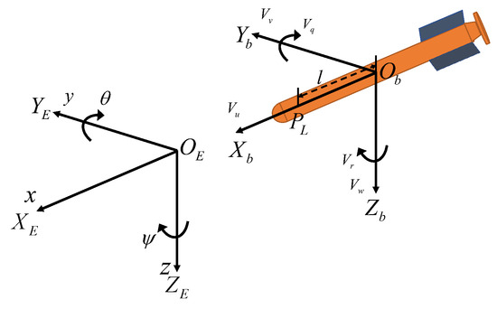
Figure 1.
Motion coordinates for an underactuated AUV.
To deal with the input saturation problem, the following auxiliary system is introduced:
where , , are positive constants, as follows:
Remark 1.
In reference [21], the auxiliary system is constructed for time-invariant systems whose system parameters do not change with time. The autonomous underwater vehicle (AUV) system in this paper is a time-varying system; that is, the system parameters change with time. In view of this difference, the auxiliary system is modified in this paper, and the auxiliary system is transformed into a time-varying system. The system parameters of the auxiliary system are designed according to the underactuated AUV’s system parameters, and the state variables η and underactuated AUV’s system parameters are introduced.
3. Controller Design
For the underactuated AUV system model, the structure of the dynamic event-triggered adaptive backstepping controller in this paper is shown in Figure 2, which is mainly composed of an auxiliary system, an adaptive backstepping controller, an input saturation limit, and a dynamic event-triggered mechanism. The auxiliary system takes the controller output difference as input and outputs some signal compensating the input saturation to the adaptive backstepping controller and the update law. The update law combines the state variables and the compensation signal to produce an estimate of the upper bound on the disturbance, and the estimate is passed to the adaptive backstepping controller. The adaptive backstepping controller output is passed to the dynamic auxiliary variable after input limitation. The dynamic event-triggered mechanism combines dynamic auxiliary variables and system state variables to trigger events and finally outputs to the control plant.
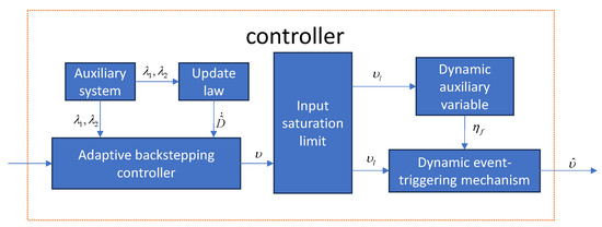
Figure 2.
Controller structure.
3.1. Adaptive Backstepping Controller Design
Before designing the controller, the following coordinate transformation is given:
- Step 1:
The derivative of the actual displacement (3) is obtained:
It can be obtained from the system (1)
By simplification, we obtain
let
we have
Derivative of , we obtain
Take the virtual control law as follows:
Let the Lyapunov function as
Derivative of , we obtain
- Step 2:
Derivative of , we obtain
The controller is designed as follows:
where , , is D estimates.
The update law is designed as follows:
where is a positive definite matrix.
Let the Lyapunov function as
Derivative of , we obtain
From Equation (21), it can be observed that are bounded. By assumption, both are bounded. Consequently, are also bounded.
Theorem 1.
For the subsystem given by the model (2), under the input signal (17) and the update law (18), we can obtain
- (1)
- (2)
Proof of Theorem 1.
From (21), it follows that the derivative of is less than zero, and are bounded. According to the LaSalle-Yoshizawa theorem, when , . therefore, .
According to (14)
where .
Therefore,
When setting and , .
namely
To analyze the stability of the auxiliary system, let the Lyapunov function be
Derivative of , we obtain
According to the following inequality
We have
Since are both diagonal positive definite matrices. Let
we have
namely
where , , represents all the eigenvalues of . Thus, we have
When for , we have . Thus,
□
It follows that the tracking error is related to . The closer the initial estimate is to the true value D, the smaller the tracking error becomes. Additionally, selecting larger values for further reduces the tracking error.
3.2. Dynamic Event-Triggered Control
Let the auxiliary variables be
where . is the event-triggered controller output (17). The trigger mechanism is designed as follows:
where .
The design of the controller is summarized in Table 1. Theorems can be obtained from the summary as follows.

Table 1.
Controller expression.
Theorem 2.
Proof of Theorem 2.
Let the Lyapunov function be as follows:
Derivative of (39), we obtain
Notice the inequality
We have
Let
We have
According to the Formula (36), it can be obtained that
Based on the above analysis, it can be concluded that after the system (1) adopts the control law (17), update law (18), and dynamic event-triggering (36), as long as are positive constants, , and , the system will be stable.
Exclusion of the Zeno behavior: We will prove that the Zeno phenomenon will not occur by using the method of reductio ad absurdum. First, we will assume that the Zeno phenomenon will occur.
where . There are infinitely many event triggers within the time interval . In the , is a fixed value, so derivative can obtain . And in , e may be 0 many times in the interval except at the beginning. Let the moment when the last e is 0 be denoted as . In , we have
where .
It follows from Lemma 2 that
Then,
Since is a continuous function and bounded by the Formula (17), the interval exists
where are the upper bounds of the three components of , respectively.
Because , a sufficient condition for making Formula (36) was established
Since , at the next triggered time, the following condition holds
So in the interval , must have
Therefore, this contradicts the assumption, as triggering cannot occur infinitely many times within the interval ; thus, the Zeno phenomenon does not occur. □
4. Simulation Results
In this section, the 5-DOF underactuated AUV model from the reference [22] is used as the simulation plant to verify the effectiveness of the proposed dynamic event-triggered adaptive backstepping controller. The model is as follows:
where
The external disturbance are
In the simulation, we adopt the controller, update law, and event-triggered mechanism as shown in Table 1 and the amplitudes of the actuators are all limited between .
In order to verify the effectiveness and adaptability of the dynamic event-triggered adaptive backstepping controller, two different tracking targets are used in the simulation experiments.
4.1. Example 1
The control objectives are set as follows:
The controller parameters are set as follows:
The initial state is taken .
The simulation results are shown in the figure. In Figure 3a, the dynamic event-triggered adaptive backstepping control and the static event-triggered adaptive backstepping control are used for experimental comparison. Figure 3b–d represents the tracking error over time in the three dimensions x, y, and z.
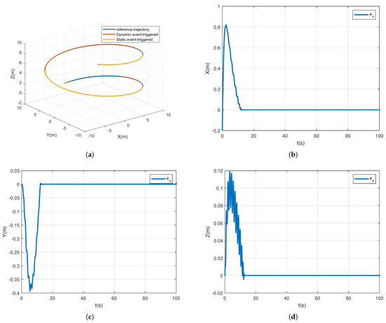
Figure 3.
Example 1 Tracking effect and error. (a) Tracking trajectory. (b) Error of the x-axis. (c) Error of the y-axis. (d) Error of the z-axis.
Figure 4a shows the estimation of the upper bound for the external disturbance. Figure 4b shows the change in the dynamic auxiliary variable.
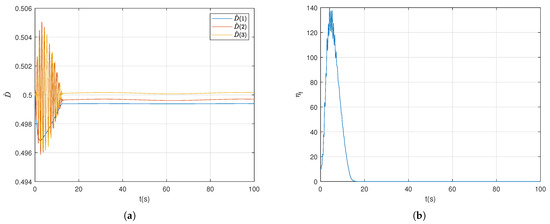
Figure 4.
Example 1 Estimation of parameters and dynamic variables. (a) Estimation of the upper bound of external disturbances. (b) Dynamic auxiliary variable.
Figure 5a–c are the controller outputs. The three terms in the figure represent the controller output, the output after limited, and the output after the event is triggered. Figure 5d represents the time interval of the trigger.
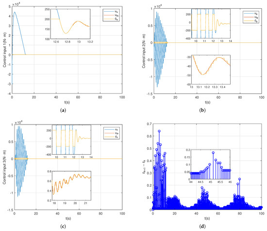
Figure 5.
Example 1 Control output and trigger time. (a) Control input 1. (b) Control input 2. (c) Control input 3. (d) Consecutive time intervals.
4.2. Example 2
The control objectives are set as follows:
The controller parameters are set as follows:
The initial state is taken .
The simulation results are shown in the figure. In Figure 6a, the dynamic event-triggered adaptive backstepping control and the static event-triggered adaptive backstepping control are used for experimental comparison. Figure 6b–d represents the tracking error over time in the three dimensions x, y, and z.
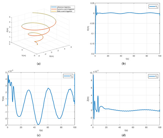
Figure 6.
Example 2 Tracking effect and error. (a) Tracking trajectory. (b) Error of the x-axis. (c) Error of the y-axis. (d) Error of the z-axis.
Figure 7a shows the estimation of the upper bound for the external disturbance. Figure 7b shows the change in the dynamic auxiliary variable.
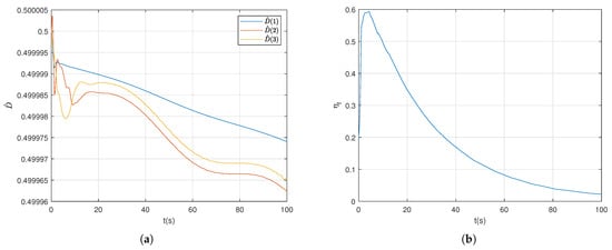
Figure 7.
Example 2 Estimation of parameters and dynamic variables. (a) Estimation of the upper bound of external disturbances. (b) Dynamic auxiliary variable.
Figure 8a–c are the controller outputs. The three terms in the figure represent the controller output, the output after limited, and the output after the event is triggered. Figure 8d represents the time interval of the trigger.
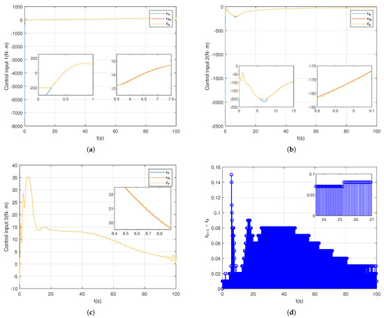
Figure 8.
Example 2 Control output and trigger time. (a) Control input 1. (b) Control input 2. (c) Control input 3. (d) Consecutive time intervals.
4.3. Discussion
It can be observed from Figure 3a and Figure 6a that both dynamic event triggering and static event triggering can track the tracking target. In order to reflect the tracking effect more intuitively, we have counted the maximum tracking error of the two algorithms in three dimensions, x, y, and z, in different cases in Table 2. Comparing the maximum error in different cases, we can see that the two algorithms have the same tracking effect. Figure 5a–c and Figure 8a–c show the process of controller calculation. Firstly, the output is given by the adaptive backstepping controller combined with the auxiliary system, then the output is obtained by limiting, and finally the output after the dynamic event is triggered. It is observed that the range of variation of the three control inputs in Example 1 is different from that in Example 2; mainly the values in the controller are different. For different tracking targets, different need to be adjusted. In the controller, are within a certain range; the larger the value of , the better the control effect, but beyond a certain range, the system will become unstable.
Table 2.
Maximum error in each dimension.
Figure 5d and Figure 8d represent the time interval between the triggering of the event. To compare the effect, we count the number of static and dynamic event-triggered executions in Table 3. The comparison shows that under the same tracking effect, the execution times of dynamic event triggering are significantly less than that of static event triggering, and the execution efficiency is higher.
Table 3.
The number of events for the two algorithms.
5. Conclusions
In this paper, a dynamic event-triggered adaptive backstepping controller is designed for a 5-DOF underactuated AUVs with input saturation and external disturbances. Firstly, the 5-DOF underactuated AUVs model was divided into the underactuated part and the actuated part, and the output was redefined according to the virtual control point. Secondly, based on the adaptive backstepping control, an auxiliary system is constructed according to the characteristics of the underactuated AUVs model to generate a series of signals to compensate for the input saturation. Then, dynamic event triggering is implemented by using state variables and controller outputs as event-triggering conditions. Finally, through theoretical analysis and simulation experiments, it is concluded that the dynamic event-triggered adaptive backstepping controller can effectively solve the input saturation problem and reduce the number of executions while making the stability error tend to zero.
In this paper, we consider how to reduce the number of executions as much as possible to improve the execution efficiency in the case of input saturation. In practice, in addition to the problem of input saturation in this paper, there are also problems such as time delay, dead zone, sensor fault (bias, zero drift, loss of accuracy, etc.), actuator fault (bias fault, gain fault, etc.), etc. Our future research direction will consider the actual situation more comprehensively and explore how to ensure the stability of the system while improving the execution efficiency under these restrictions. After the theoretical verification, we are ready to improve the experimental conditions and carry out the physical experiment.
Author Contributions
Conceptualization, F.Q. and J.C.; methodology, F.Q.; software, F.Q. and Y.Z.; writing, F.Q. and A.W. All authors have read and agreed to the published version of the manuscript.
Funding
This research received no external funding.
Data Availability Statement
The original contributions presented in this study are included in the article. Further inquiries can be directed to the corresponding author.
Conflicts of Interest
The authors declare no conflicts of interest.
References
- Jiang, Y.; Zhang, K.; Zhao, M.; Qin, H. Adaptive meta-reinforcement learning for AUVs 3D guidance and control under unknown ocean currents. Ocean Eng. 2024, 309, 118498. [Google Scholar] [CrossRef]
- Ma, D.; Chen, X.; Ma, W.; Zheng, H.; Qu, F. Neural Network Model-Based Reinforcement Learning Control for AUV 3-D Path Following. IEEE Trans. Intell. Veh. 2024, 9, 893–904. [Google Scholar] [CrossRef]
- Cui, R.; Yang, C.; Li, Y.; Sharma, S. Adaptive Neural Network Control of AUVs with Control Input Nonlinearities Using Reinforcement Learning. IEEE Trans. Syst. Man Cybern.-Syst. 2017, 47, 1019–1029. [Google Scholar] [CrossRef]
- Zhang, H.; Hu, Y.; Song, Z. Event-triggered adaptive fault-tolerant control with pre-specified performance for AUVs trajectory tracking. Ocean Eng. 2024, 313, 119372. [Google Scholar] [CrossRef]
- Li, Z.; Wang, M.; Ma, G.; Zou, T. Adaptive reinforcement learning fault-tolerant control for AUVs with thruster faults based on the integral extended state observer. Ocean Eng. 2023, 271, 113722. [Google Scholar] [CrossRef]
- Cui, R.; Zhang, X.; Cui, D. Adaptive sliding-mode attitude control for autonomous underwater vehicles with input nonlinearities. Ocean Eng. 2016, 123, 45–54. [Google Scholar] [CrossRef]
- Ding, W.; Zhang, L.; Zhang, G.; Wang, C.; Chai, Y.; Mao, Z. Research on 3D trajectory tracking of underactuated AUV under strong disturbance environment. Comput. Electr. Eng. 2023, 111, 108924. [Google Scholar] [CrossRef]
- Gong, H.; Er, M.J.; Liu, Y.; Ma, C. Three-dimensional optimal trajectory tracking control of underactuated AUVs with uncertain dynamics and input saturation. Ocean Eng. 2024, 298, 116757. [Google Scholar] [CrossRef]
- Gong, H.; Er, M.J.; Liu, Y. Fuzzy adaptive optimal fault-tolerant trajectory tracking control for underactuated AUVs with input saturation. Ocean Eng. 2024, 311, 118940. [Google Scholar] [CrossRef]
- Luo, W.; Cheng, B. Disturbance suppression and NN compensation based trajectory tracking of underactuated AUV. Ocean Eng. 2023, 288, 116172. [Google Scholar] [CrossRef]
- Zhou, Q.; Wang, L.; Wu, C.; Li, H.; Du, H. Adaptive Fuzzy Control for Nonstrict-Feedback Systems with Input Saturation and Output Constraint. IEEE Trans. Syst. Man Cybern. Syst. 2017, 47, 1–12. [Google Scholar] [CrossRef]
- Li, J.; Fan, Y.; Liu, J. Distributed fixed-time formation tracking control for multiple underactuated USVs with lumped uncertainties and input saturation. ISA Trans. 2024, 154, 186–198. [Google Scholar] [CrossRef]
- Yang, C.; Huang, D.; He, W.; Cheng, L. Neural Control of Robot Manipulators with Trajectory Tracking Constraints and Input Saturation. IEEE Trans. Neural Netw. Learn. Syst. 2021, 32, 4231–4242. [Google Scholar] [CrossRef]
- Ge, X.; Han, Q.L.; Zhang, X.M.; Ding, D. Dynamic Event-triggered Control and Estimation: A Survey. Int. J. Autom. Comput. 2021, 18, 857–886. [Google Scholar] [CrossRef]
- Sedghi, L.; Ijaz, Z.; Noor-A-Rahim, M.; Witheephanich, K.; Pesch, D. Machine Learning in Event-Triggered Control: Recent Advances and Open Issues. IEEE Access 2022, 10, 74671–74690. [Google Scholar] [CrossRef]
- Yan, Y.; Wang, R.; Yu, S.; Wang, C.; Li, T. Event-triggered output feedback sliding mode control of mechanical systems. Nonlinear Dyn. 2022, 107, 3543–3555. [Google Scholar] [CrossRef]
- Ye, H.; Song, Y.; Zhang, Z.; Wen, C. Global Dynamic Event-Triggered Control for Nonlinear Systems with Sensor and Actuator Faults: A Matrix-Pencil-Based Approach. IEEE Trans. Autom. Control 2024, 69, 2007–2014. [Google Scholar] [CrossRef]
- Xiao, J.; Liu, Y.; An, Y. Adaptive dynamic event-triggered fault tolerant control for uncertain strict-feedback nonlinear systems. Eur. J. Control 2024, 79, 101096. [Google Scholar] [CrossRef]
- Xing, L.; Wen, C. Dynamic event-triggered adaptive control for a class of uncertain nonlinear systems. Automatica 2023, 158, 111286. [Google Scholar] [CrossRef]
- Hu, X.; Gong, Q.; Han, J.; Zhu, X.; Yang, H.; Wang, M. Dynamic event-triggered composite anti-disturbance fault-tolerant tracking control for ships with disturbances and actuator faults. Ocean Eng. 2023, 280, 114662. [Google Scholar] [CrossRef]
- Zhou, J.; Wen, C. Adaptive Backstepping Control of Uncertain Systems; Springer: Berlin/Heidelberg, Germany, 2008. [Google Scholar]
- Zhang, X.; Jiang, K. Backstepping-based adaptive control of underactuated AUV subject to unknown dynamics and zero tracking errors. Ocean Eng. 2024, 302, 117640. [Google Scholar] [CrossRef]
- Shojaei, K.; Arefi, M.M. On the neuro-adaptive feedback linearising control of underactuated autonomous underwater vehicles in three-dimensional space. IET Control Theory Appl. 2015, 9, 1264–1273. [Google Scholar] [CrossRef]
- Consolini, L.; Tosques, M. A Minimum Phase Output in the Exact Tracking Problem for the Nonminimum Phase Underactuated Surface Ship. IEEE Trans. Autom. Control 2012, 57, 3174–3180. [Google Scholar] [CrossRef]
Disclaimer/Publisher’s Note: The statements, opinions and data contained in all publications are solely those of the individual author(s) and contributor(s) and not of MDPI and/or the editor(s). MDPI and/or the editor(s) disclaim responsibility for any injury to people or property resulting from any ideas, methods, instructions or products referred to in the content. |
© 2025 by the authors. Licensee MDPI, Basel, Switzerland. This article is an open access article distributed under the terms and conditions of the Creative Commons Attribution (CC BY) license (https://creativecommons.org/licenses/by/4.0/).