Fuzzy PDC-Based LQR Sliding Neural Network Control for Two-Wheeled Self-Balancing Cart

Abstract

This paper proposes a fuzzy PDC (parallel distributed compensation)-based LQR (Linear Quadratic Regulator) sliding neural network methodology to control a two-wheeled self-balancing cart. Firstly, a mathematical model of a two-wheeled self-balancing cart is described to explain some parameter meanings. Then, we detail how a simulation was implemented according to these reasonable parameter settings under the fuzzy PDC-based LQR sliding neural network control algorithm. Secondly, the algorithm is developed by setting four controllable LQR controllers. Then, a ReLU-based neural network (ReNN) is developed to tune the fuzzy degrees for these four LQR controllers. This means that an intelligent controller is designed by using the fuzzy PDC concept. Subsequently, a sliding surface is designed, and the sliding mode is utilized to compensate and enhance its stability. Simulation was conducted to verify the feasibility of this proposed algorithm. The simulation results demonstrate good effectiveness and stability. Finally, a cart equipped with an STM32 MCU (microcontroller unit) was implemented to verify the feasibility of this proposed algorithm. The empirical experimental results show that the two-wheeled self-balancing cart exhibited good self-balancing performance and stability.

1. Introduction

Fuzzy parallel distributed compensation (fuzzy PDC) was proposed many years ago, and it has become a critical, effective, and vibrant research method for some nonlinear systems [1,2,3,4]. Based on these reasons, a series of studies on the development of fuzzy PDC have been greatly promoted. In [1], a design method for a fuzzy controller based on the Takagi–Sugeno (T-S) fuzzy model was proposed. It is a document with an important theoretical basis in the development of fuzzy PDC. This design principle of fuzzy PDC was explained in detail, including how to use the parallel compensation method to design a fuzzy controller based on the T-S fuzzy model to cope with nonlinear systems. In [2], the fuzzy PDC method was used to control a robot and simulation was performed to obtain good verifications of the system, which proved the excellence of fuzzy PDC; meanwhile, the results could meet the requirements of the system. In [3], the authors proposed a particle swarm optimization (PSO) algorithm combined with the fuzzy PDC method to design robust and stable quadratic optimal fuzzy controllers to improve the stability and performance of the control system. In [4], a fuzzy TS-PDC controller was proposed to cope with power systems. It can reduce the number of fuzzy rules to simplify the complex fuzzy rule base. In summary, fuzzy PDC has resulted in both theoretical improvement and practical application progress. The continuous research results on fuzzy PDC and the relevant theoretical papers have made fuzzy PDC become an increasingly promising control technology in the control theory area.

The LQR (Linear Quadratic Regulator) control methodology has been used for a long time, and it has very excellent performance for linear systems [5]. But when we focus on uncertain nonlinear systems, some research has been proposed which has only used sliding mode neural networks to tune some important parameters to, for example, generate different control forces and then to achieve good performances. Sliding mode control [6,7,8,9] is used to generate a sliding surface and then to make the system trajectories bounded in the stable region cope with some parameter uncertainties and external disturbances. Neural networks [10,11,12,13] have abilities to tune different weightings of neurons to, for example, achieve good performance. When sliding mode and neural networks are integrated into sliding mode neural networks, they can be used to control some applications such as robotics, two-wheeled self-balancing carts, etc. [14,15,16,17].

The nonlinear model predictive control (NMPC) approach has demonstrated significant efficacy in trajectory control for robots, robotic arms, and remote operation systems [18,19,20]. By integrating receding horizon optimization with system dynamics, NMPC enables the precise tracking of complex motion profiles while handling constraints in diverse applications. However, despite its strengths in model-driven scenarios, NMPC often faces challenges in real-time implementation on low-cost embedded hardware—such as microcontroller units (MCUs)—due to its high computational demand and reliance on accurate system modeling. In contrast, the proposed method addresses these critical limitations by prioritizing real-time performance, hardware compatibility, and robustness to model uncertainties for self-balancing cart systems. Unlike NMPC’s iterative optimization, our approach combines pre-computed LQR gains with adaptive neural network tuning and sliding mode control, reducing computational latency to within microcontroller capabilities. This hybrid architecture ensures stable operation under un-modeled dynamics (e.g., wheel friction variations or external disturbances) without requiring online model updates.

The advantages of this framework were empirically validated through both numerical simulations and physical experiments (see Section 6). Results show that the proposed method achieved smaller control cycles on an STM32 MCU, outperforming NMPC in comparable low-power setups. These findings highlight its practical suitability for real-world robotics and automation applications where cost, latency, and resilience are paramount.

The contribution of this paper is calculating the LQR gain value, K, under different states and then assigning K to form a fuzzy PDC control algorithm based on the adjustment parameters calculated by the sliding mode neural network under different states to stabilize the system and obtain good performance.

2. Two-Wheeled Self-Balancing Cart Mathematical Model

The mathematical model of the two-wheeled self-balancing cart is used to understand the wheel model, as shown in Figure 1. The mathematical model of forward motion around the center of mass, p, of the cart can be expressed as follows [21,22]:

$$\begin{array}{c}\ddot{x}=-{\displaystyle \frac{M^2{l}^{2}g}{Q_{eq}}}{\theta }_P+{\displaystyle \frac{J_P+M{l}^2+Mlr}{Q_{eq}r}}(T_R+T_L)\\ {\ddot{\theta }}_P=\frac{Ml(M+2m+2I/r^2)g}{Q_{eq}}{\theta }_P-{\displaystyle \frac{Ml/r+M+2m+2I/r^2}{Q_{eq}}}(T_R+T_L)\end{array}$$

(1)

where $Q_{eq}$ is defined as

$$Q_{eq}=J_{P}M+(J_P+M{l}^2)(2m+2I/r^2)$$

(2)

The parameters of model are defined as follows:

• $x$: the horizontal displacement of the center, O, of the chassis of the cart;
• $M$: the mass of the vehicle body (kg);
• $l$: the distance from center of mass to center of chassis (m);
• $J_P$: the moment of inertia of the vehicle body when rotating around the center of mass ($\mathrm{kg}\ast {\mathrm{m}}^2$);
• ${\theta }_P$: the angle between the vehicle body and the vertical direction (rad);
• $m$: the wheel mass (kg);
• $r$: the radius of the wheel (m);
• $T_R$: the output torque of the right wheel motor ($\mathrm{N}\cdot \mathrm{m}$);
• $T_L$: the output torque of the left wheel motor ($\mathrm{N}\cdot \mathrm{m}$);
• $I$: the moment of inertia of the wheel ($\mathrm{kg}\ast {\mathrm{m}}^2$);
• $g$: the gravity acceleration magnitude (9.8 $\mathrm{m}/{\mathrm{s}}^2$).

From (1) and (2), the state space expression can be obtained as follows:

$$\begin{array}{c}\dot{\mathit{x}}=\mathit{Ax}+\mathit{Bu}\\ \mathit{y}=\mathit{Cx}+\mathit{Du}\end{array}$$

(3)

where

$$\begin{gathered} \mathit{A}=\left[\begin{array}{cccc}0& 1& 0& 0\\ 0& 0& A_{23}& 0\\ 0& 0& 0& 1\\ 0& 0& A_{43}& 0\end{array}\right]; \mathit{B}=\left[\begin{array}{cc}0& 0\\ B_{21}& B_{22}\\ 0& 0\\ B_{41}& B42\end{array}\right]; \mathit{C}=\left[\begin{array}{cccc}1& 0& 0& 0\\ 0& 0& 1& 0\end{array}\right]; \\ \mathit{D}=\left[\begin{array}{cc}{d}_{11}& d_{12}\\ d_{21}& d_{22}\end{array}\right]; \mathit{x}=\left[\begin{array}{c}x\\ \dot{x}\\ {\theta }_P\\ {\dot{\theta }}_P\end{array}\right]; \mathit{u}=\left[\begin{array}{c}{u}_1\\ u_2\end{array}\right]; \mathit{y}=\left[\begin{array}{c}x\\ {\theta }_P\end{array}\right] \end{gathered}$$

(4)

3. LQR Controller Design

From Equations (1)–(4), based on the introduced mathematical model, this section discusses how to use the LQR control method to stabilize the system initially and then ensure that our proposed control law can guarantee the foundation of stability when facing nonlinear systems. Consider a controller which is represented as $\mathit{u}=-\mathit{Kx}$, where $\mathit{K}\in R^{2\times 4}$ is the LQR controller gain matrix. After substituting $\mathit{u}$ into (3), the following equation can be obtained:

$$\begin{gathered} \dot{\mathit{x}}=Ax-B\mathit{Kx} \\ =(A-B\mathit{K})\mathit{x} \end{gathered}$$

(5)

where $\mathit{x}={\left[\begin{array}{cccc}x& \dot{x}& {\theta }_P& {\dot{\theta }}_P\end{array}\right]}^T$, where $x$ is the position, $\dot{x}$ is the velocity, ${\theta }_P$ is the angle, and the ${\dot{\theta }}_P$ is the angular velocity. $u$ is the output torque, but in practice, it needs to be converted into the motor’s PWM output. The objective is to design a state feedback matrix, $\mathit{K}$, to keep the angle of the two-wheeled self-balancing cart vertical, and the displacement will return to the original point. So, we utilize the LQR derivation method to design $\mathit{K}$, which will be introduced below; this implies that the control error should be zero. Based on the LQR theory [5], the cost function $J$ is defined as follows. The control purpose is to design the $\mathit{Q}$ and $\mathit{R}$ matrices so as to minimize $J$:

$$J={\displaystyle \int [{\mathit{x}}^{\mathit{T}}\mathit{Qx}+{\mathit{u}}^{\mathit{T}}\mathit{Ru}]dt}$$

(6)

where $\mathit{Q}$ and $\mathit{R}$ are weighting matrices for the states and control forces, respectively. The diagonal elements $q_i$ in $\mathit{Q}$ represent the importance attached to the corresponding error component $x_i$; if we want the convergence to be faster, then a larger weight coefficient will be set. Similarly, the diagonal elements $r_i$ in $\mathit{R}$ represent restrictions on the corresponding input components $u_i$; in general case, the weight coefficient should be set to smaller value to avoid making the system unstable and uncontrollable.

In order to achieve an optimal $\mathit{K}$, the cost function $J$ should be minimized. Based on the optimal control theory [6,23], the optimal solution can be obtained by the means of algebraic methods or differential methods. A common approach is to solve the Riccati equation [20]. We can solve the following Riccati equation:

$${\mathit{A}}^{\mathit{T}}\mathit{P}+\mathit{PA}-{\mathit{PBR}}^{-1}{\mathit{B}}^{\mathit{T}}\mathit{P}+\mathit{Q}=0$$

(7)

where $\mathit{P}$ is a symmetric and positive definite state feedback gain matrix of a square dimension of 4. If the positive definite matrix $\mathit{P}$ exists, then the optimal controller gain matrix $\mathit{K}$ can be obtained as follows [5,17]:

$${\mathit{K}}_{LQR}={\mathit{R}}^{-1}{\mathit{B}}^{\mathit{T}}\mathit{P}$$

(8)

Finally, the LQR controller can be expressed as

$${\mathit{u}}_{LQR}=-{\mathit{K}}_{LQR}\mathit{x}$$

(9)

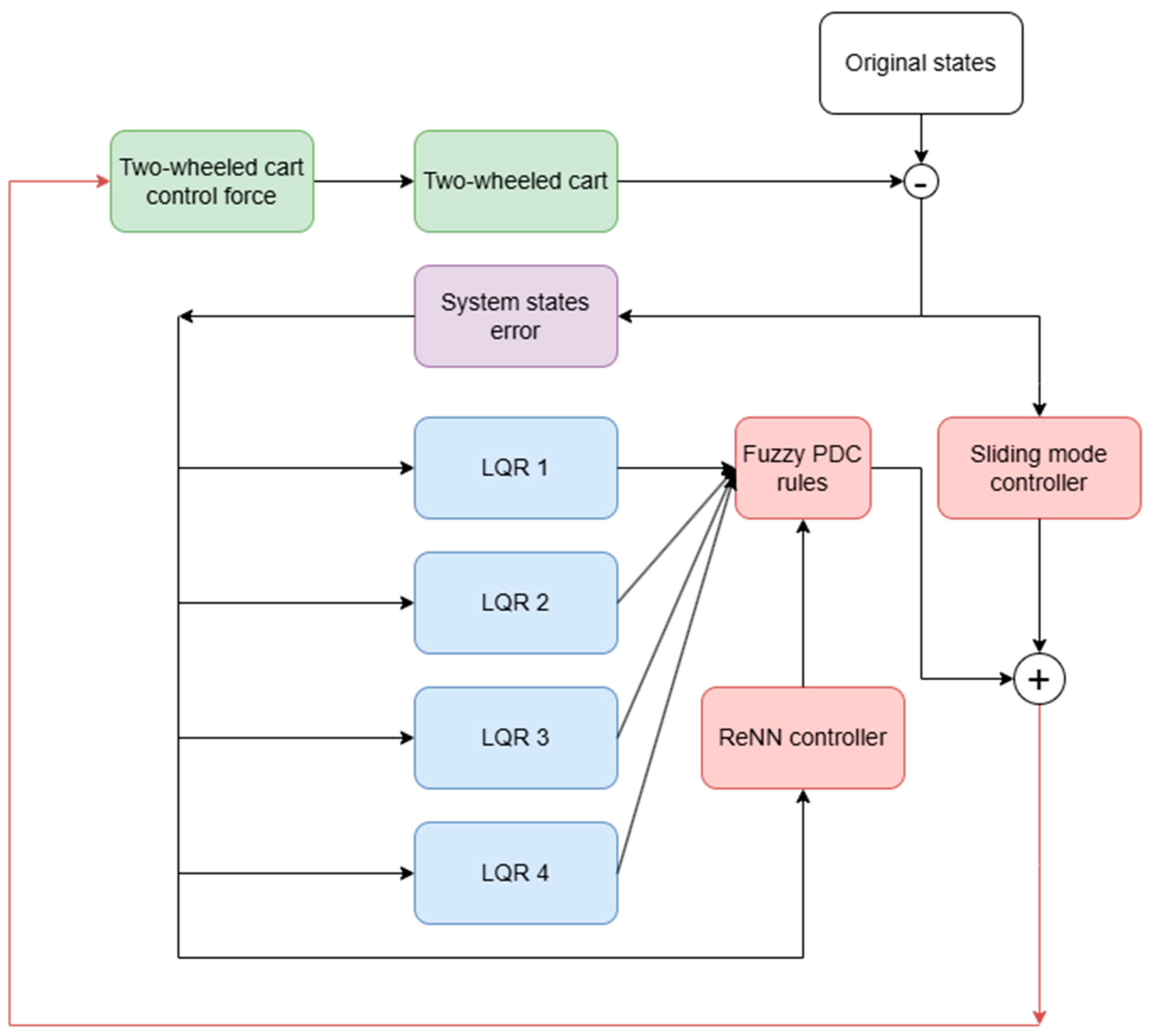
4. Fuzzy PDC-Based Sliding Neural Network Design

In order to cope with the uncertainty and nonlinear characteristics of the system, the sliding mode control method and a neural network are needed for tuning some parameters of fuzzy PDC. The overall design concept diagram is proposed in Figure 2.

4.1. Sliding Controller Design

Sliding control [6,7,8,9] is designed by using a pair of suitable defined sliding surfaces as

$$s_1=\dot{x}+{\lambda }_{1}x$$

(10)

$$s_2={\dot{\theta }}_P+{\lambda }_2{\theta }_P$$

(11)

where ${\lambda }_1$ and ${\lambda }_2$ are positive constants. The time derivatives of (10) and (11) are obtained as

$${\dot{s}}_1=\ddot{x}+{\lambda }_1\dot{x}$$

(12)

$${\dot{s}}_2={\ddot{\theta }}_P+{\lambda }_2{\dot{\theta }}_P$$

(13)

From (1)–(4), (12) and (13), the simplified nonlinear model can be derived as

$${\dot{s}}_1=A_{23}{\theta }_P+(B_{21}{u}_1+B_{22}{u}_2)+{\lambda }_1\dot{x}$$

(14)

$${\dot{s}}_2=A_{43}{\theta }_P+(B_{41}{u}_1+B_{42}{u}_2)+{\lambda }_2{\dot{\theta }}_P$$

(15)

There is an error between the reasonable values of $u_1$ and $u_2$. We can make the following mathematical expression.

$$u_1=u_2+\Delta u_2$$

(16)

Substituting (16) into (14) and (15) yields the following mathematical expression:

$${\dot{s}}_1=A_{23}{\theta }_P+(B_{21}+B_{22})u_1-B_{22}\Delta u_2+{\lambda }_1\dot{x}$$

(17)

$${\dot{s}}_2=A_{43}{\theta }_P+(B_{41}+B_{42})u_2+B_{41}\Delta u_2+{\lambda }_2{\dot{\theta }}_P$$

(18)

By using the sliding mode theorem [6], we assume that $\Delta u_2=0$; then, the sliding mode conditions should be ${\dot{s}}_1=0$ and ${\dot{s}}_2=0$ [6,7,8,9]. An equivalent control law can be obtained as

$$u_{eq1}={\displaystyle \frac{-A_{23}{\theta }_P-{\lambda }_1\dot{x}}{B_{21}+B_{22}}}$$

(19)

$$u_{eq2}={\displaystyle \frac{-A_{43}{\theta }_P-{\lambda }_2{\dot{\theta }}_P}{B_{41}+B_{42}}}$$

(20)

According to the sliding mode control theorem, switching control terms should be added to (19) and (20) to satisfy the Lyapunov stability condition [24]. $u_1$ and $u_2$ are designed as the following control law.

$$u_1=u_{eq1}+u_{sm1}$$

(21)

$$u_2=u_{eq2}+u_{sm2}$$

(22)

From (10)–(13), the Lyapunov function is defined as

$$V(s_1,s_2)={\displaystyle \frac{1}{2}}{s}_1^2+{\displaystyle \frac{1}{2}}{s}_2^2$$

(23)

From (14)–(22), according to the Lyapunov stability theorem, the derivation process is the following:

$$\begin{array}{l}\dot{V}=s_1{\dot{s}}_1+s_2{\dot{s}}_2\\ =s_1[A_{23}{\theta }_P+(B_{21}+B_{22})u_1-B_{22}\Delta u_2+{\lambda }_1\dot{x}]+s_2[A_{43}{\theta }_P+(B_{41}+B_{42})u_2+B_{41}\Delta u_2+{\lambda }_2{\dot{\theta }}_P]\\ =s_1[A_{23}{\theta }_P+(B_{21}+B_{22})(u_{eq1}+u_{sm1})-B_{22}\Delta u_2+{\lambda }_1\dot{x}]+s_2[A_{43}{\theta }_P+(B_{41}+B_{42})(u_{eq2}+u_{sm2})\\ +B_{41}\Delta u_2+{\lambda }_2{\dot{\theta }}_P]\\ =s_1[(B_{21}+B_{22})(u_{sm1})-B_{22}\Delta u_2]+s_2[(B_{41}+B_{42})(u_{sm2})+B_{41}\Delta u_2]\end{array}$$

(24)

Now, we set $u_{sm1}$ and $u_{sm2}$ as follows:

$$u_{sm1}={\displaystyle \frac{-{\epsilon }_1\mathrm{sgn}(s_1)}{B_{21}+B_{22}}}$$

(25)

$$u_{sm2}={\displaystyle \frac{-{\epsilon }_2\mathrm{sgn}(s_2)}{B_{41}+B_{42}}}$$

(26)

where $\mathrm{sgn}(\cdot )$ denotes a sign function with a boundary of 0.5 to mitigate the chattering effect, and ${\epsilon }_1$ and ${\epsilon }_2$ are positive bound numbers. In (24), we consider $B_{22}\Delta u_2$ and $B_{41}\Delta u_2$ very small bounded quantities. They represent uncertainty, nonlinearities, and disturbances. We assume that they have small bounded relationships, ${\epsilon }_1\ge \left|B_{22}\Delta u_2\right|$ and ${\epsilon }_2\ge \left|B_{41}\Delta u_2\right|$, with $s_1$ and $s_2$, respectively, so (24) can be derived as the following equation.

$$\begin{array}{l} \dot{V}=s_1[-{\epsilon }_1\mathrm{sgn}(s_1)-B_{22}\Delta u_2]+s_2[-{\epsilon }_2\mathrm{sgn}(s_2)+B_{41}\Delta u_2]\\ =[-{\epsilon }_1\left|s_1\right|-B_{22}\Delta u_2{s}_1]+[-{\epsilon }_2\left|s_2\right|+B_{41}\Delta u_2{s}_2]\\ \le -[{\epsilon }_1+B_{22}\Delta u_2]\left|s_1\right|-[{\epsilon }_2-B_{41}\Delta u_2]\left|s_2\right|\le 0\end{array}$$

(27)

Through the above Equation (27), the stability and robustness of the system are proven and guaranteed simultaneously.

4.2. Fuzzy PDC-Based LQR Controller Design

According to the equivalent control $u_{eq1}$ and $u_{eq2}$ of the sliding mode proposed in the previous section, its control value will encounter a lot of interference in physical implementation. Therefore, we design a neural network in the following section to propose a method which can monitor and determine the weight for choosing between the LQR controllers. That is, the weights of each LQR controller must be calculated by the neural network discussed later. Here, the fuzzy PDC method is introduced to deduce every degree of the four LQRs.

The concept of fuzzy PDC is the following [1,2,3,4]:

$$\begin{array}{l}Rule i: IF x(t) is {\mu }_{i1} \dots and {\theta }_P(t) is {\mu }_{in}\\ \begin{array}{c} THEN \dot{\mathit{x}}(t)={\mathit{A}}_i\mathit{x}(t)+{\mathit{B}}_{i}u(t)\end{array}\end{array}$$

(28)

where ${\mathit{A}}_i$ are system matrices and ${\mathit{B}}_i$ are input matrices; i = 1,2,3,4; there are four IF–THEN fuzzy rules in this paper; and ${\mu }_{ij}$ are the fuzzy singleton. Then, the fuzzy PDC output rules can be established.

$$\begin{array}{l}Rule j: IF x(t) is {\mu }_{j1} \dots and {\theta }_P(t) is {\mu }_{jn}\\ \begin{array}{c} THEN u_j(t)=-{\mathit{K}}_j\mathit{x}(t)\end{array}\end{array}$$

(29)

for $j=1,2,3,4$, where ${\mathit{K}}_j\in R^{2\times 4}$ are state feedback matrix gains of LQR.

Through different state simulations, we assign different fuzzy degree to two states,$x$ and ${\theta }_P$, and we denote them as ${\mu }_i$ where $i=1,2,3,4$. Then, through defuzzification, we obtain the final degree value as follows.

$$u_{Fuzzy-PDC-LQR}={\displaystyle \frac{{\mu }_1{K}_{LQR1}+{\mu }_2{K}_{LQR2}+{\mu }_3{K}_{LQR3}+{\mu }_4{K}_{LQR4}}{{\mu }_1+{\mu }_2+{\mu }_3+{\mu }_4}}$$

(30)

The ReNN (discussed in Section 4.3 and Section 5) dynamically adjusts the fuzziness values of the LQR controller.

4.3. Neural Network Controller Design

The ReLU (Rectified Linear Unit) in neural networks has several notable features [25,26,27,28]. It has simple and efficient computation ability. Its activation function is very simple; that is, $f(x)=\max (0,x)$. During forward propagation, it only needs to determine whether the input is greater than zero or not, which reduces the computational load and can speed up the training process. Meanwhile, it helps alleviate the vanishing gradient problem. When the input is greater than zero, the derivative of the ReLU is 1, enabling the gradient to be effectively propagated back to previous layers. Finally, for a large number of negative inputs, the output of the neuron is zero. Only a portion of neurons are activated; this reduces the interdependence between neurons, mitigating the over-fitting risk. Figure 3 depicts a three-layer neural network (ReNN). It consists of an input layer, a hidden layer, and a output layer. The energy function is minimized using the slope to obtain the optimal weights of the ReNN. The following introduces the meaning and basic functions of each layer of the ReNN:

(a)

Input Layer: Each node within this layer is related to the net input and net output values, which are, respectively, denoted as $x_i$ and $y_{i,j}$.

$$ne{t}_i=x_i$$

(31)

$$y_{i,j}=f_{i,j}(ne{t}_i)=ne{t}_i, i=1,2,3,\cdots ,m, \mathrm{and} j=1,2,3,\cdots ,m$$

(32)

Here, $x_i$ stands for the i-th input to the node of Layer 1, and $m$ represents the number of input variables. All the link weights in this layer are assigned a value of 1.

(b)

Hidden Layer: Each node in this layer performs activation using the ReLU function, which is defined as $\mathrm{Re}Lu(x)=\max (0,x)$ [22,23,24,25,26,27,28]. The derivative of the ReLU is 1 when the input number is greater than zero; otherwise, it is equal to 0. The ReLU will be used as the activation function for the j-th node of the i-th input.

$${net}_{ij}=\max (0,y_{i,j})$$

(33)

The number of neurons in this layer determines the number of neurons that are triggered. The larger the number of neurons is, the more important the rule is. Therefore, it will affect the output weights of the four LQR controllers in fuzzy PDC. The triggered node (denoted by $\prod$) plays a key role at this time because it multiplies the input signal and produces an output specific to the j-th rule node. The expression is defined by the following equation:

$$y_{jk}=\underset{ij}{{\displaystyle \Pi }}ne{t}_{ij}, i=j=1,2,3,4$$

(34)

(c)

Output Layer: It consists of two nodes, one for LQR and the other for the sliding mode controller, which is responsible for performing the key operation of calculating the percentage of the two controllers. Among these nodes, we have a specific node labeled $\Sigma$, which learns and memorizes the optimal percentage output by monitoring all input system states signals. This summation process is represented by the following equation:

$${net}_k=\sum _j{w}_{jk}{y}_{jk}$$

(35)

$$u_k=f_k\left({net}_k\right)={net}_k, k=1,2,3,4$$

(36)

A more elaborate description of the components involved in this calculation can be further provided as follows.

• $w_{jk}$: The link weight denoting the strength of the output action corresponding to the output of the j-th column in relation to the k-th rule.
• $y_{jk}$: The j-th input to the node of layer.
• $m$: The total number of output nodes.
• $u_k$: The k-th column output of the ReNN controller.

Based on the gradient theory [10,11,12,13], we utilize a single neuron to derive the equations within the neural network. To tune the weights of the ReNN, the energy function and the cost function are defined as follows so as to carry out the gradient operation:

$$E(u,w)={\displaystyle \frac{1}{2}}{(u^{*}-u)}^2$$

(37)

The gradient calculus of $E$ with respect to $w$ can be obtained as follows:

$$\Delta w_j=-\eta {\displaystyle \frac{\partial E}{\partial w_j}}=-\eta ({\displaystyle \frac{\partial E}{\partial u}}\ast {\displaystyle \frac{\partial u}{\partial w_j}})=(u^{*}-u)\ast y_k$$

(38)

where $\eta$ is learning rate. Likewise, the update law for the activation layer can be derived as

$$\Delta w_i=-\eta \underset{i}{\Sigma }{\displaystyle \frac{\partial E}{\partial w_i}}=-\eta ({\displaystyle \frac{\partial E}{\partial y_j}}\ast {\displaystyle \frac{\partial y_j}{\partial w_j}})=y_j{\displaystyle \sum _j{w}_j}\ast (u^{\ast }-u)\ast y_j$$

(39)

After the calculation by the ReNN, the output weights $w_i,i=1,2,3,4$ correspond to 4 fuzzy degrees of fuzzy PDC in (30) which are ${\mu }_i,i=1,2,3,4$ for $x$; in the same way, the output weights of $w_j,j=1,2,3,4$ correspond to 4 fuzzy degrees of fuzzy PDC which are ${\mu }_j,j=1,2,3,4$ for ${\theta }_P$, respectively.

From (25), (26) and (30), the total control laws are designed as follows:

$$u_1=u_{Fuzzy-PDC-LQR1}+u_{sm1}$$

(40)

$$u_2=u_{Fuzzy-PDC-LQR2}+u_{sm2}$$

(41)

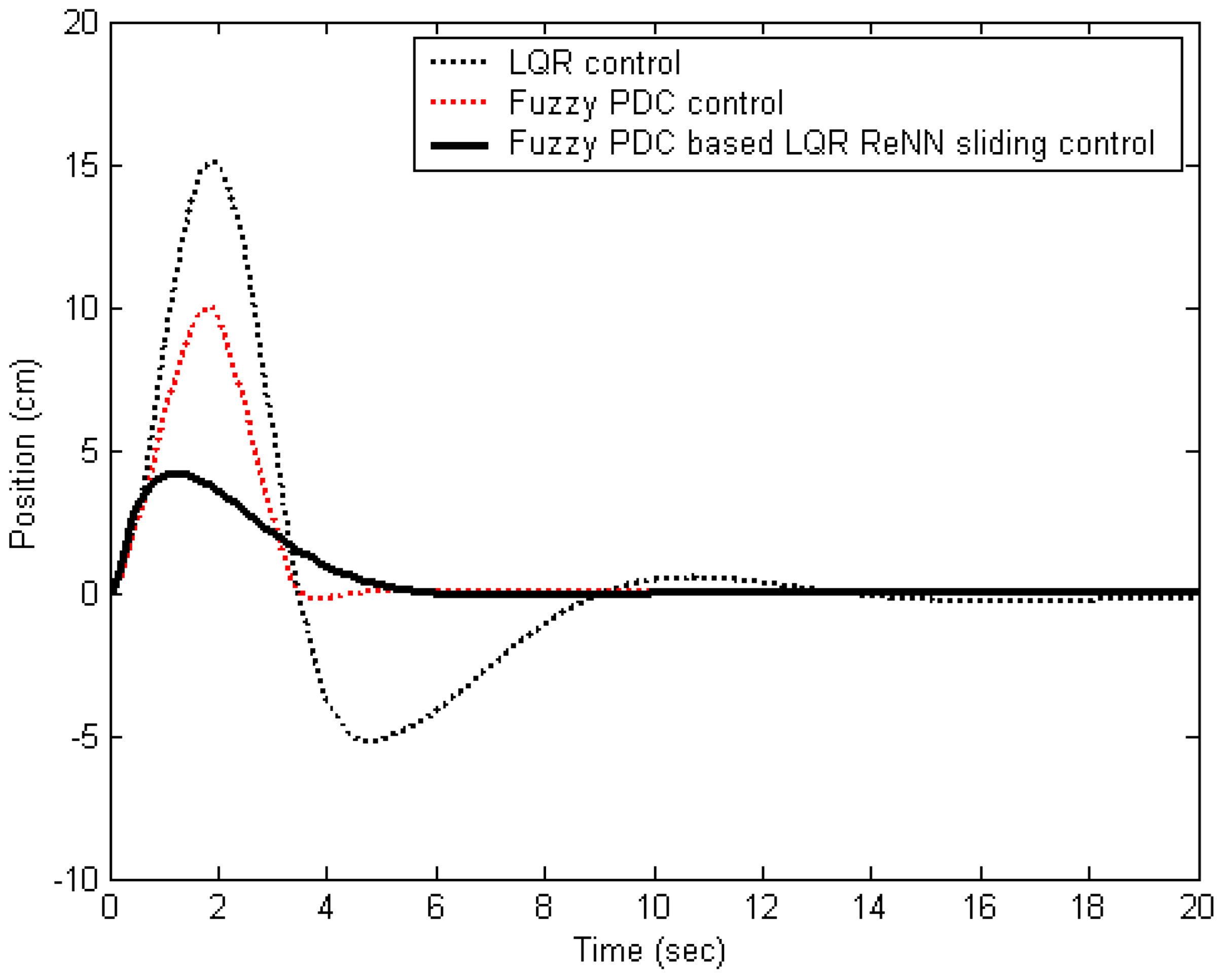
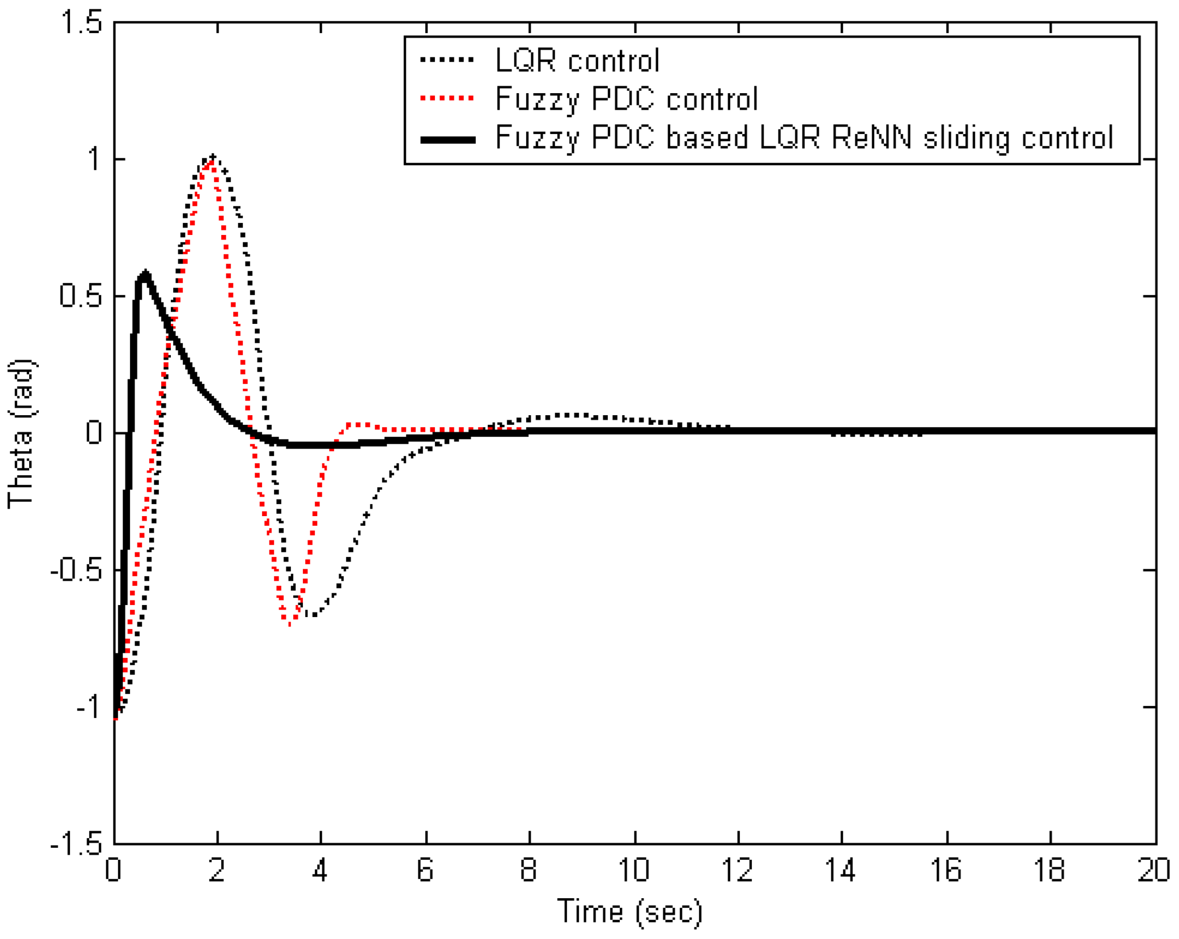
5. Simulation Results

According to the mathematical models of Equations (1) and (2), the simulation parameters of the two-wheeled self-balancing cart model were set as follows: $m=0.035$; $r=0.0672/2$; $I=0.5\ast m\ast r^2$; $M=0.757-2\ast m$; and $l=0.5\ast 0.0903$. By using Matlab R14 software [29,30], after the Q and R matrices were set, four LQR gain matrices K could then be obtained as follows.

$$Q_1=\left[\begin{array}{cccc}2000& 0& 0& 0\\ 0& 0& 0& 0\\ 0& 0& 0& 0\\ 0& 0& 0& 2000\end{array}\right];R_1=\left[\begin{array}{cc}2& 0\\ 0& 2\end{array}\right];K_1=\left[\begin{array}{cccc}-22.36& -36.44& -276& -27.93\\ -22.36& -36.44& -276& -27.93\end{array}\right]$$

(42)

$$Q_2=\left[\begin{array}{cccc}4000& 0& 0& 0\\ 0& 0& 0& 0\\ 0& 0& 0& 0\\ 0& 0& 0& 4000\end{array}\right];R_2=\left[\begin{array}{cc}3& 0\\ 0& 3\end{array}\right];K_2=\left[\begin{array}{cccc}-25.82& -40.07& -283.41& -31.23\\ -25.82& -40.07& -283.41& -31.23\end{array}\right]$$

(43)

$$Q_3=\left[\begin{array}{cccc}3000& 0& 0& 0\\ 0& 0& 0& 0\\ 0& 0& 0& 0\\ 0& 0& 0& 3000\end{array}\right];R_3=\left[\begin{array}{cc}4& 0\\ 0& 4\end{array}\right];K_3=\left[\begin{array}{cccc}-19.36& -33.25& -270& -25.15\\ -19.36& -33.25& -270& -25.15\end{array}\right]$$

(44)

$$Q_4=\left[\begin{array}{cccc}20000& 0& 0& 0\\ 0& 0& 0& 0\\ 0& 0& 0& 0\\ 0& 0& 0& 20000\end{array}\right];R_4=\left[\begin{array}{cc}5& 0\\ 0& 5\end{array}\right];K_4=\left[\begin{array}{cccc}-44.72& -59.91& -331.06& -50.2\\ -44.72& -59.91& -331.06& -50.2\end{array}\right]$$

(45)

Based on the four K values calculated above in (42)–(45), a simulation comparison was performed based on the control laws (30), (40) and (41). The results are shown in Figure 4 and Figure 5. Figure 6 is shown as the control force for the small cart. As shown in the results, the design method of the fuzzy PDC-based LQR ReNN sliding control proposed outperforms the traditional LQR method in terms of effectiveness. While the algorithm integrates multiple control techniques (fuzzy PDC, LQR, sliding mode, and neural network), its hybrid architecture and application to two-wheeled self-balancing carts represent a non-trivial innovation with distinct advantages over my prior work.

The ReNN was trained on 2 million synthetic samples generated from 10,000 simulation trials with diverse initial states. Each sample comprised state variables and corresponding optimal fuzzy PDC weights obtained from LQR simulations. As shown in Figure 7, the training and validation MSE curves are illustrated. The training MSE converged to 0.023, with a validation MSE of 0.028, highlighting strong generalization capability. To alleviate overfitting, early stopping was implemented, which effectively maintained a small gap between training and validation errors. Figure 8 and Figure 9 depict the weight changes during the training process. Figure 8 corresponds to the weight dynamics for $x$, while Figure 9 shows those for ${\theta }_P$. From the dynamic trajectory changes in these figures, it is evident that the ReNN could indeed dynamically adjust the fuzziness values of the LQR controller.

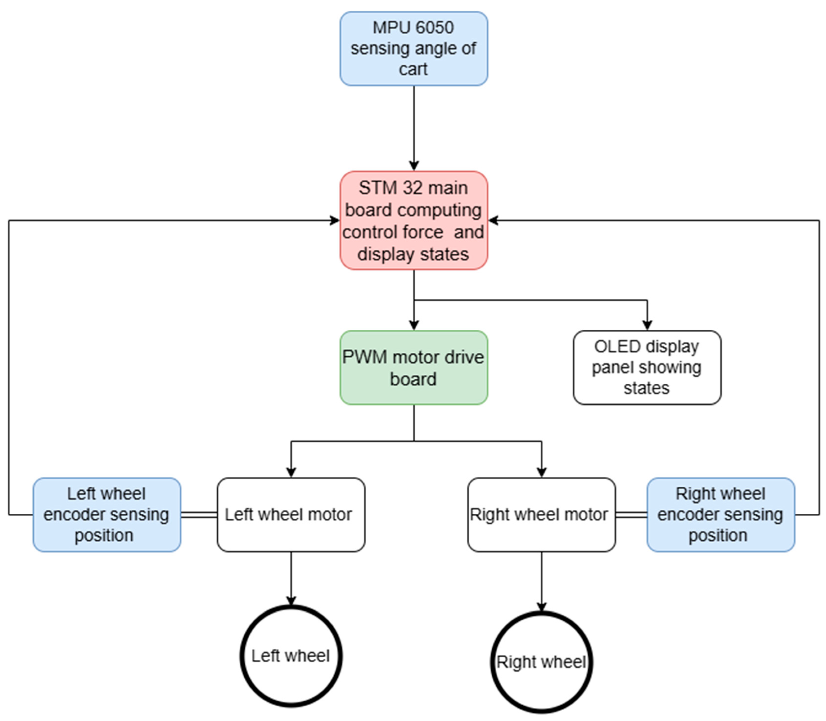
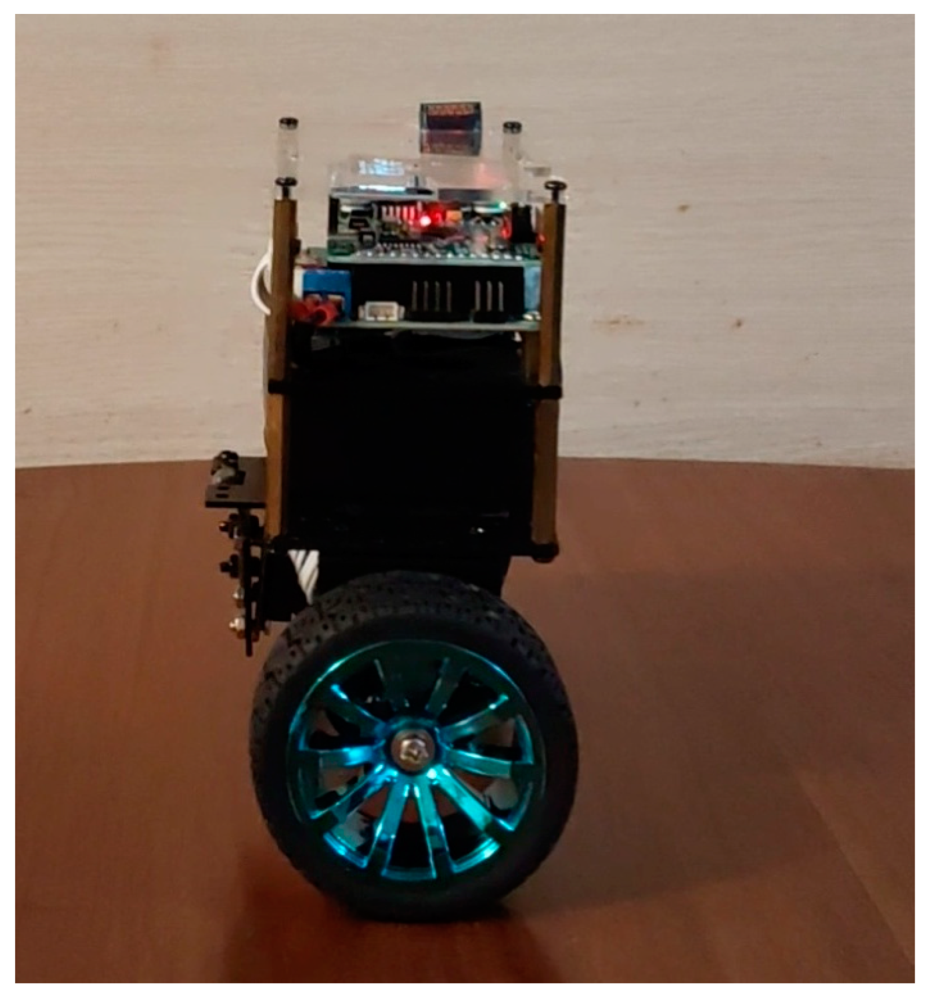
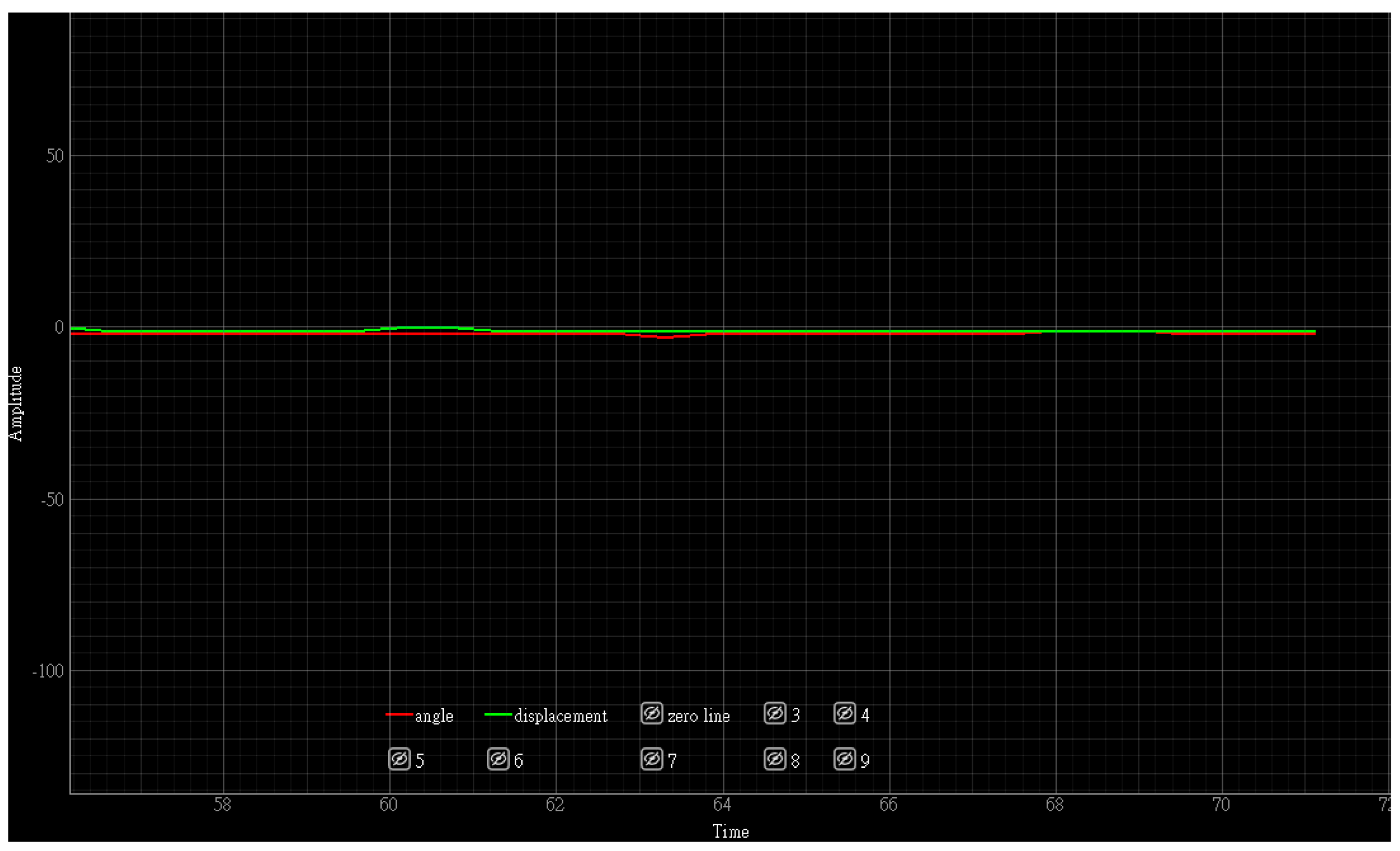
6. Experiment Results

The hardware used in the experiment included a two-wheeled self-balancing cart produced by Wheeltech Inc. (Dongguan, China) [22]. The main board photo is shown in Figure 10. An image taken after connecting the main board to other components such as wheels, the drive board, etc., is shown in Figure 11. The cart consisted of two wheels, a main board, a sensor board, an OLED display panel, a Bluetooth board, a battery, and a motor drive board. The algorithm proposed in this paper could be verified using the two-wheeled self-balancing cart. The block diagram of the implemented cart is introduced in Figure 12. The main board was mainly manufactured with an STM32 series MCU chip (Geneva, Switzerland) [31]. The states of the cart body such as angle and position were sensed by an MPU 6050 board [22]; the sensing signals were encoded and then sent to the main board. After that, algorithm calculations from the control law were carried out and the PWM signals were sent to the motor drive board to control the wheel motors to, for example, let the cart to be stable and self-balancing. By using a real implementation of the cart, after it was powered on, it was verified that the proposed fuzzy PDC-based LQR sliding neural network control methodology is effective and very stable. The diagram is shown in Figure 13. Meanwhile, the sensed angle changing line could be viewed on a computer monitor by the means of the Bluetooth board on the cart. It is shown in Figure 14.

7. Conclusions

This paper develops a fuzzy PDC-based LQR sliding neural network methodology to control a two-wheeled self-balancing cart. Firstly, a simulation was conducted to verify the feasibility of this proposed algorithm. The simulation demonstrated very good effectiveness and stability. Then, a cart equipped with an STM32 MCU was implemented to verify the feasibility of this proposed algorithm. The results of the empirical experiment show that good self-balancing performance and stability were exhibited.

References

1. Wang, H.O.; Tanaka, K.; Griffin, M.F. An Approach to Fuzzy Control of Nonlinear Systems: Stability and Design Issues. IEEE Trans. Fuzzy Syst. 1996, 4, 14–23. [Google Scholar]
2. Lin, C.M.; Mon, Y.J. A Fuzzy-PDC-Based Control for Robotic Systems. Inf. Sci. 2001, 137, 135–155. [Google Scholar] [CrossRef]
3. Pal, D.; Chatterjee, A.; Rakshit, A. Robust-Stable Quadratic-Optimal Fuzzy-PDC Controllers for Systems with Parametric Uncertainties: A PSO Based Approach. Eng. Appl. Artif. Intell. 2018, 70, 38–51. [Google Scholar]
4. Alshammari, B.; Ben Salah, R.; Kahouli, O.; Kolsi, L. Design of Fuzzy TS-PDC Controller for Electrical Power System via Rules Reduction Approach. Symmetry 2020, 12, 2068. [Google Scholar] [CrossRef]
5. Kalman, R.E. A New Approach to Linear Filtering and Prediction Problems. J. Basic Eng. 1960, 82, 35–45. [Google Scholar]
6. Slotine, J.J.E.; Li, W. Applied Nonlinear Control; Prantice-Hall: Englewood Cliffs, NJ, USA, 1991. [Google Scholar]
7. Edwards, C.; Spurgeon, S.K. Sliding Mode Control: Theory and Applications; CRC Press: Boca Raton, FL, USA, 1998. [Google Scholar]
8. Zhang, Z.; Yang, X.; Wang, W.; Chen, K.; Cheung, N.C.; Pan, J. Enhanced Sliding Mode Control for PMSM Speed Drive Systems Using a Novel Adaptive Sliding Mode Reaching Law Based on Exponential Function. IEEE Trans. Ind. Electron. 2024, 71, 11978–11988. [Google Scholar] [CrossRef]
9. Ma, S.; Zhao, J.; Xiong, Y.; Wang, H.; Yao, X. Sliding-Mode Control of Linear Induction Motor Based on Exponential Reaching Law. Electronics 2024, 13, 2352. [Google Scholar] [CrossRef]
10. Ge, S.S.; Hang, C.C.; Lee, T.H.; Zhang, T. Stable Adaptive Neural Network Control; Springer Science & Business Media: Berlin/Heidelberg, Germany, 2013; Volume 13. [Google Scholar]
11. Zheng, C.; Hu, C.; Yu, J.; Wen, S. Saturation Function-Based Continuous Control on Fixed-Time Synchronization of Competitive Neural Networks. Neural Netw. 2024, 169, 32–43. [Google Scholar] [CrossRef]
12. Tam, P.; Ros, S.; Song, I.; Kang, S.; Kim, S. A Survey of Intelligent End-to-End Networking Solutions: Integrating Graph Neural Networks and Deep Reinforcement Learning Approaches. Electronics 2024, 13, 994. [Google Scholar] [CrossRef]
13. Li, M.; Xu, J.; Wang, Z.; Liu, S. Optimization of the Semi-Active-Suspension Control of BP Neural Network PID Based on the Sparrow Search Algorithm. Sensors 2024, 24, 1757. [Google Scholar] [CrossRef]
14. Simon, J. Fuzzy Control of Self-Balancing, Two-Wheel-Driven, SLAM-Based, Unmanned System for Agriculture 4.0 Applications. Machines 2023, 11, 467. [Google Scholar] [CrossRef]
15. Tsai, C.-C.; Huang, H.-C.; Lin, S.-C. Adaptive Neural Network Control of a Self-Balancing Two-Wheeled Scooter. IEEE Trans. Ind. Electron. 2010, 57, 1420–1428. [Google Scholar] [CrossRef]
16. Nghia, V.B.V.; Van Thien, T.; Son, N.N.; Long, M.T. Adaptive Neural Sliding Mode Control for Two Wheel Self Balancing Robot. Int. J. Dynam. Control 2022, 10, 771–784. [Google Scholar] [CrossRef]
17. Mon, Y.-J. Tikhonov-Tuned Sliding Neural Network Decoupling Control for an Inverted Pendulum. Electronics 2023, 12, 4415. [Google Scholar] [CrossRef]
18. Hu, Y.; Su, H.; Zhang, L.; Miao, S.; Chen, G.; Knoll, A. Nonlinear Model Predictive Control for Mobile Robot Using Varying-Parameter Convergent Differential Neural Network. Robotics 2019, 8, 64. [Google Scholar] [CrossRef]
19. Zhang, J.; Zhang, X.; Cheng, Y.; Cheng, Y.; Zhang, Q.; Lu, K. Nonlinear Model Predictive Control (NMPC) based shared autonomy for bilateral teleoperation in CFETR Remote Handling. Nuclear Eng. Technol. 2024, 56, 4437–4445. [Google Scholar] [CrossRef]
20. Wang, J.; Liu, Z.; Chen, H.; Zhang, Y.; Zhang, D.; Peng, C. Trajectory Tracking Control of a Skid-Steer Mobile Robot Based on Nonlinear Model Predictive Control with a Hydraulic Motor Velocity Mapping. Appl. Sci. 2023, 14, 122. [Google Scholar] [CrossRef]
21. Grasser, F.; D’Arrigo, A.; Colombi, S.; Rufer, A.C. JOE: A Mobile, Inverted Pendulum. IEEE Trans. Ind. Electron. 2002, 49, 107–114. [Google Scholar] [CrossRef]
22. Wheeltec Inc. Two-Wheeled Self Balancing Cart Technical Development Manual; Wheeltec Inc.: Dongguan, China, 2025; Available online: www.wheeltec.net (accessed on 20 April 2025).
23. Kwakernaak, H.; Sivan, R. Linear Optimal Control Systems; Wiley-Interscience: New York, NY, USA, 1972; Volume 1, p. 608. [Google Scholar]
24. Wang, M.; He, X.; Li, X. Self-Triggered Impulsive Control for Lyapunov Stability of Nonlinear Systems in Discrete Time. IEEE Trans. Cybern. 2024, 54, 4852–4858. [Google Scholar] [CrossRef]
25. Fei, W.; Dai, W.; Li, C.; Zou, J.; Xiong, H. On Centralization and Unitization of Batch Normalization for Deep ReLU Neural Networks. IEEE Trans. Signal Process. 2024, 72, 2827–2841. [Google Scholar] [CrossRef]
26. Liang, X.; Xu, J. Biased ReLU Neural Networks. Neurocomputing 2021, 423, 71–79. [Google Scholar] [CrossRef]
27. Barbu, A. Training a Two-Layer ReLU Network Analytically. Sensors 2023, 23, 4072. [Google Scholar] [CrossRef] [PubMed]
28. Sooksatra, K.; Rivas, P. Dynamic-Max-Value ReLU Functions for Adversarially Robust Machine Learning Models. Mathematics 2024, 12, 3551. [Google Scholar] [CrossRef]
29. Mathworks Inc. MATLAB R14 User’s Manual; Mathworks Inc.: Natick, MA, USA, 2004; Available online: https://www.mathworks.com/ (accessed on 20 April 2025).
30. TeraSoft Inc. MATLAB R 14 User’s Manual; TeraSoft Inc.: Taipei, Taiwan, 2004; Available online: https://www.terasoft.com.tw/ (accessed on 20 April 2025).
31. STMicroelectronics. STM32F103xx Reference Manual; ST Microelectronics: Geneva, Switzerland, 2025; Available online: https://www.st.com.cn/content/st_com/zh.html (accessed on 20 April 2025).
Figure 1. The concept diagram of two-wheeled self-balancing cart.
Electronics 14 01842 g001
Figure 2. The design concept diagram of fuzzy PDC-based LQR ReNN sliding mode control for a two-wheeled self-balancing cart.
Electronics 14 01842 g002
Figure 3. The ReNN diagram.
Electronics 14 01842 g003
Figure 4. The simulation results of x (cart position).
Electronics 14 01842 g004
Figure 5. The simulation results of θ P (cart angle).
Electronics 14 01842 g005
Figure 6. The simulation results of u 1 + u 2 (cart control torque).
Electronics 14 01842 g006
Figure 7. Training and validation MSE curves.
Electronics 14 01842 g007
Figure 8. Weighting change diagram for x .
Electronics 14 01842 g008
Figure 9. Weighting change diagram for θ P .
Electronics 14 01842 g009
Figure 10. A physical photo of the main board.
Electronics 14 01842 g010
Figure 11. A physical photo of the cart.
Electronics 14 01842 g011
Figure 12. A block diagram of the hardware of the implementation of the cart.
Electronics 14 01842 g012
Figure 13. A photo of the real implementation of the cart.
Electronics 14 01842 g013
Figure 14. A diagram of the angle changing line.
Electronics 14 01842 g014
Disclaimer/Publisher’s Note: The statements, opinions and data contained in all publications are solely those of the individual author(s) and contributor(s) and not of MDPI and/or the editor(s). MDPI and/or the editor(s) disclaim responsibility for any injury to people or property resulting from any ideas, methods, instructions or products referred to in the content.