Adaptive Real-Time Convergence Estimation for Enhancing Reliability of Time Synchronization in Distributed Energy Monitoring System

Abstract

In distributed energy monitoring systems, precise time synchronization is paramount for efficient data acquisition and energy management. With the high penetration of new energy sources, the distributed energy monitoring system will evolve into a complex heterogeneous network utilizing various short-range wireless communication technologies. Therefore, wireless communication-based time synchronization technologies will be widely applied, and it is important for the distributed energy monitoring system to be aware of the current time synchronization errors as this is crucial for accurate data processing. Our findings propose the first real-time convergence estimation method using an adaptive real-time convergence estimation (ARCE) algorithm, which can accurately estimate the current network time synchronization error and convergence status in real time. This ARCE algorithm is based on synchronization error and distribution of both synchronous and asynchronous time synchronization algorithm. The actual distributions of synchronization error are analyzed and evaluated using a significant amount of experimental results. According to the experimental results and simulations, ARCE can effectively detect the convergence state for all the comparisons. Therefore, ARCE can be used to evaluate the reliability of timestamps in data acquisition. Moreover, it can be utilized to enhance the adaptive capability of time synchronization algorithms, which could be robust and scalable for a large-scale and randomly deployed wireless networks.

1. Introduction

Time synchronization is a critical issue and a necessary condition in most of the distributed systems including industrial Internet of Things [1,2,3], communication systems [4], localization systems [5,6], smart grids [7], data acquisition [8], time-sensitive networking [9,10], and control systems [11,12]. In particular, precise time synchronization is crucial for efficient energy management in campus energy internet systems. Accurate time synchronization ensures that energy resources are managed optimally, reducing waste and improving overall system efficiency. In recent years, wireless sensor networks (WSNs) have been employed in IoT, making time synchronization in WSNs an exceedingly popular topic. Due to the distributed and energy-constrained nature of WSNs, the node’s capability for communication is limited. Moreover, the topology of these wireless networks is too dynamic. Therefore, the time synchronization problem remains an inherent challenge in WSNs.

In the literature, accuracy, energy-efficiency, scalability, robustness, and convergence rate are commonly used as the performance metrics for the WSN time synchronization algorithm. However, it is difficult for the time synchronization algorithm to optimize all of these performance metrics simultaneously. For instance, centralized or clustered time synchronization algorithms, e.g., RBS [13], CESP [14], and cluster-based approaches [15,16] focus on the improvement of accuracy and energy-efficiency while ignoring scalability and robustness. To overcome such ignored performance, flooding time synchronization approaches have been introduced, e.g., FTSP [17], FCSA [18], PulseSync [19], PISync [20], and RMTS [21,22]; however, the topological changes still pose challenges to the robustness of the time synchronization in dynamic WSNs. In consensus-based methods [23], e.g., ATS [24], MTS [25], GTSP [26], MACTS [27], and DCTS [28], the scalability and the robustness of time synchronization are greatly improved compared to any other algorithms, while the convergence rate is much slower than the flooding approach [29,30].

In addition, the existing time synchronization algorithms employ a fixed structure and presupposed operating mechanism. This is a bottleneck of the algorithm to optimize the performance in real time, serving as a critical metric for synchronous convergence. According to the experimental results in [20,21,22,27], it can be found that the performance of time synchronization algorithms highly depends on the topology. For instance, the accuracy of flooding time synchronization mainly depends on the diameter of WSNs, and the density of a network will affect its robustness. Thus, the accuracy and convergence rate of consensus-based time synchronization are affected by the shape and density of the network.

1.1. Challenge Analysis

We observe that the performance of existing methods may not be consistent in randomly deployed and large-scale WSN applications, and the major challenges are as follows.

(1)

The performance highly depends on the shape of the network topology. There are specific requirements for the shape of the network to achieve better performance. For instance, the average consensus approach (e.g., ATS, MACTS) can meet better performance targets in grid networks than in line networks; the flooding approach (e.g., FTSP, PulseSync, and RMTS) can set up time synchronization faster than average consensus in line networks, while it has no significant advantage in grid networks.

(2)

The performance cannot be estimated in real time. Specifically, the time synchronization algorithm cannot evaluate the synchronization status of networks, and the algorithm cannot repair the time synchronization performance once the shape of the network is changed. Considering the average consensus approach, once the network shape evolves from a grid to line, then the performance will be significantly reduced.

(3)

The synchronization parameters, e.g., synchronization time interval and coefficient, are always fixed values, and the parameters must be configured before the deployment of the time synchronization algorithm. Thus, setting the right parameters for a randomly deployed network can be difficult, and the network cannot reset the parameters to meet the changes of the topology.

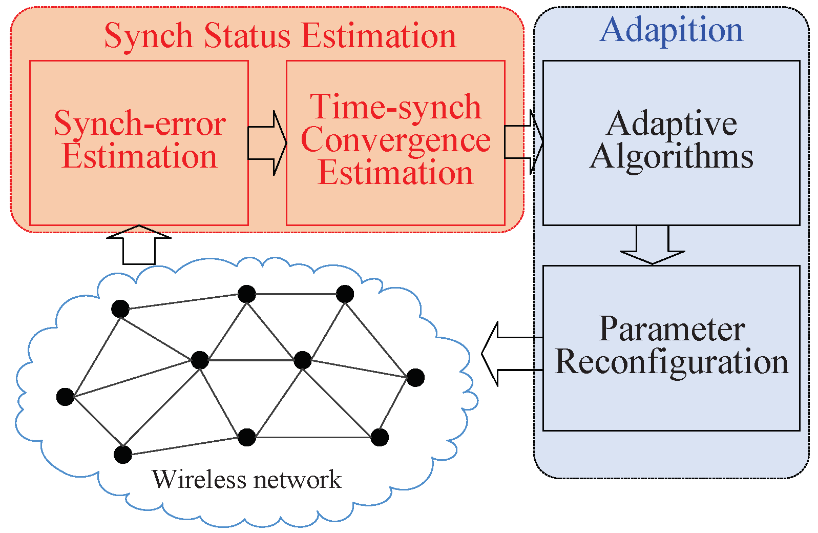
Therefore, developing a novel time synchronization algorithm which can achieve consistent performance in different shapes of network topology will be very valuable. Thus, the time synchronization algorithm should be an adaptive approach, as shown in Figure 1.

There are two components in an adaptive approach: synchronization status estimation and adaptation. The algorithm first estimates the synchronization status, including synchronization errors and convergence status. Then, it adjusts the synchronization parameters to match the shape of the topology.

1.2. Motivation and Contributions

In this paper, we are interested in synchronization status estimation, focus on convergence detection based on synchronization error estimation, and propose adaptive real-time convergence estimation (ARCE) to provide a reference for future studies on adaptive time synchronization.

Synchronization error is a key parameter for evaluating the performance of a time synchronization algorithm, commonly used to indicate the accuracy of the algorithm. Similarly, to analyze the convergence of time synchronization, a threshold of synchronization error is used to detect the convergence time [24,27]. Furthermore, changes in synchronization error are used to describe the scalability and robustness of an algorithm after interference occurs [24,25]. In a previous study on MACTS [27], to reduce by-hop error accumulation and communication costs caused by time information forwarding, a simple convergence estimation based on synchronization error estimation was used to drive the multi-hop controller of MACTS. As a result, MACTS can achieve a fast convergence rate with few communication increments.

Based on the analysis of existing time synchronization algorithms, it can be found that synchronization errors show significant differences before and after convergence, and the convergence of time synchronization can be summarized as two phases, i.e., setup and hold-on. At the hold-on phase, time synchronization is convergent, where the synchronization errors are stable random variables with a constant mean in the time interval. Therefore, the proposed ARCE is developed based on a synchronization characteristic estimator and a convergence probability estimator, and it is evaluated based on flooding and average consensus-based time synchronization algorithms, separately. Also, the implications of ARCE for the average consensus time synchronization algorithm (MACTS) are discussed.

The following aspects of ARCE are noteworthy:

• The proposed ARCE uses clock offset estimation of the time synchronization algorithm to indicate instantaneous local synchronization errors and estimates the convergence time of synchronization errors in real time.
• It can detect a sudden change in local synchronization errors and indicates the out-of-synchronization status of local network, where a significant clock offset estimation may be ignored in the time synchronization algorithm based on one-way broadcast [21]. Hence, ARCE is beneficial for accurate clock parameter estimation.
• It is a self-adaptive and real-time convergence detector which can adapt to changes in random variable delay and the environment. Meanwhile, it can start based on a loose initial condition.

Therefore, the proposed ARCE can be simply embedded into a time synchronization algorithm in which clock offset estimation is employed and can be deployed without any prior experimental results. Considering large-scale and randomly deployed WSNs, ARCE is easy to implement and improves the robustness of distributed time synchronization approaches.

1.3. Organization

The remainder of this paper is organized as follows. We present the system model in Section 2 and analyze the synchronization error in Section 3. ARCE is presented and analyzed in Section 4. The evaluation of ARCE is shown in Section 5. The implications are analyzed in Section 6. Finally, conclusions are drawn in Section 7.

2. System Model

The WSN is modeled as a graph $\mathcal{G}=(\mathcal{V},\mathcal{E})$, where $\mathcal{V}=\{1,2,\dots ,n\}$ represents the nodes of the WSN and $\mathcal{E}$ defines the available communication links. The set of neighbors for $v_i$ is ${\mathcal{N}}_i=\{j\mid (i,j)\in \mathcal{E},i\ne j\}$, where nodes $v_i$ and $v_j$ belong to $\mathcal{V}$, and $j\in {\mathcal{N}}_i$.

2.1. Clock Model

For the time synchronization algorithm, we define the hardware clock notion $H\left(t\right)$ as

$$H\left(t\right)={\int }_0^{t}h\left(\tau \right)d\tau ,$$

(1)

where $h\left(\tau \right)$ is the hardware frequency, i.e., clock speed, of the clock. The parameter $h\left(\tau \right)$ is an inherent attribute of the crystal oscillator and cannot be changed. Every node considers itself to have the ideal clock frequency (i.e., nominal frequency); thus, $h\left(\tau \right)$ is fixed to a hardware clock, i.e., $h\left(\tau \right)=1$. Considering the time synchronization in WSNs, a timer that is commonly used as a hardware clock generator counts the number of pulses in the crystal oscillator.

The logical clock $L\left(t\right)$ is given by

$$L\left(t\right)=\phi \left(t\right)\times H\left(t\right)+\theta \left(t_0\right),$$

(2)

where $\phi \left(t\right)$ is a logical relative clock rate multiplier and initialized as 1. To counteract the effect of clock skew, a time synchronization algorithm continuously adjusts $\phi \left(t\right)$ to speed up or slow down the local $L\left(t\right)$. The parameter $L\left(t\right)$ is used to supply the global time service for synchronization applications in WSNs. Variable $t_0$ is the moment that the node is powered on, and parameter $\theta \left(t_0\right)$ is the initial relative clock offset. We further describe the updated model of $L\left(t\right)$ as

$$L^{+}\left(t\right)=L\left(\tau \right)+(H\left(t\right)-H\left(\tau \right))\times {\phi }_i^j+{\theta }_i^j,(t>\tau )$$

(3)

where ${\theta }_i^j$ and ${\phi }_i^j$ are the relative clock offset and relative clock rate between arbitrary nodes $v_i$ and $v_j$, respectively.

Now, the parameters ${\theta }_i^j$ and ${\phi }_i^j$ in (3) are expressed as

$$\begin{array}{cc}\hfill {\theta }_i^j& =L_j\left(t\right)-L_i\left(t\right)\hfill \end{array}$$

(4)

$$\begin{array}{cc}\hfill {\phi }_i^j& ={\displaystyle \frac{H_j\left(t\right)-H_j(t-\tau )}{H_i\left(t\right)-H_i(t-\tau )}},\tau >0,\hfill \end{array}$$

(5)

where $v_j$ is a reference node. In addition, the relative clock offset estimation, denoted as ${\widehat{\theta }}_i^j$, is calculated by real-time timestamps of $L\left(t\right)$. Additionally, we estimate the relative clock rate by the real-time timestamp of $H\left(t\right)$.

2.2. Sync-Error Model

(1)

Local synchronization error. The synchronization error between two adjacent nodes is denoted as local synchronization error and is expressed as

$$E_l\left(t\right)=\underset{i,j\in {\mathcal{N}}_i}{sup}\{L_i\left(t\right)-L_j\left(t\right)\},$$

(6)

where node $v_i\in \mathcal{G}$, and $v_j$ is the neighbor of $v_i$.

(2)

Global synchronization error. This is used to describe the synchronization error between an arbitrary pair of nodes in $\mathcal{G}$ and is expressed as

$$E_g\left(t\right)=\underset{i,j\in \mathcal{N}}{sup}\{L_i\left(t\right)-L_j\left(t\right)\}$$

(7)

where $v_i$ and $v_j$ are not necessarily adjacent nodes.

2.3. Convergence Time

According to the existing study, convergence status is defined as the moment that the sync error is below the preset threshold. Specifically, the convergence time is calculated off-line based on the measured synchronization error. Here, $T_C$ is defined as convergence time, and it is given by

$$T_C={L\left[t_1\right]}_{E\left(t\right)<E_{\max }},t_1<t<\infty$$

(8)

where $E_{\max }$ is the presupposed synchronization error threshold. By using $E_l\left(t\right)$ or $E_g\left(t\right)$ in Equation (8), $T_C$ indicates the local and global convergence status, respectively.

3. Synchronization Error

According to (3), substituting Equation (3) into Equations (6) and (7) leads to the conclusion that parameter E in (6) and (7) highly depends on ${\phi }_i^j$ and ${\theta }_i^j$. Thus, the clock parameter estimations ${\widehat{\theta }}_i^j$ and ${\widehat{\phi }}_i^j$ are the key issues for the time synchronization algorithm, and the changes in sync error are mainly caused by estimation errors. In other words, it is reasonable to analyze sync error by using ${\phi }_i^j$ and ${\theta }_i^j$.

3.1. Analysis on Sync Error

Estimation error is unavoidable in clock parameter estimation due to the latency of timestamp creation and message exchange. Most time synchronization algorithms use periodic re-synchronization to counteract clock drift. Considering a pair of adjacent nodes $v_i$ and $v_j$, the sync error is given by

$$E_{i,j}\left(t\right)=E_{i,j}^{\widehat{\theta }}+E_{i,j}^{\widehat{\phi }}\times t,t\in (0,T),$$

(9)

where T is the re-synchronization interval of the time synchronization; parameter $E_{i,j}^{\widehat{\theta }}$, which includes the delay D, is the estimation error of clock offset estimation, i.e., $E_{i,j}^{\widehat{\theta }}={\theta }_i^j-\widehat{{\theta }_i^j}$; and parameter $E_{i,j}^{\widehat{\phi }}$ is the estimation error of clock skew estimation, i.e., $E_{i,j}^{\widehat{\phi }}={\phi }_i^j-\widehat{{\phi }_i^j}$.

Clock skew estimation error $E_{i,j}^{\widehat{\phi }}$: This error highly depends on the distribution of delay. Specifically, the bound of most of the proposed clock skew based on Gaussian delay is a proportional function of $\sigma$. For instance, in [31,32], $E_{i,j}^{\widehat{\phi }}$ is given by a delay-independent function, where the standard deviation of delay plays a major role.

Clock offset estimation error $E_{i,j}^{\widehat{\theta }}$: According to [21], $E_{i,j}^{\widehat{\theta }}$ is totally dependent on the variable delay D. For instance, in the time synchronization approaches based on the one-way broadcast model, $E_{i,j}^{\widehat{\theta }}$ is given by

$$E_{i,j}^{\widehat{\theta }}=D.$$

(10)

In addition, for the two-way message exchange model-based protocol, we write

$$E_{i,j}^{\widehat{\theta }}\approx {\displaystyle \frac{D_u-D_v}{2}},$$

(11)

where $D_u$ and $D_v$ are the uplink and downlink delay, respectively.

Actual variable delay D: As the analysis in [17], the distribution of D highly depends on the implementation of timestamp creation, and the typical delay varies across different testbeds. Most existing clock parameter maximum likelihood estimation methods use a distribution function to model D. Specifically, Gaussian and exponential distributions are the most commonly used delay models. According to the experimental results in [33], the main portion of actual delay is Gaussian, i.e., $D\sim N(\mu ,\sigma )$, where $\mu \approx 3.3$ µs and ${\sigma }^2\approx 0.0049$.

In light of the above discussion, $E_{i,j}\left(t\right)$ is Gaussian and depends on the distribution of D. According to (9), if $E_{i,j}^{\widehat{\phi }}$ and t are small enough, the formula $E_{i,j}^{\widehat{\phi }}\times t\to 0$. In addition, as discussed in [33], if $E_{i,j}^{\widehat{\phi }}\times t$ is smaller than the clock resolution (granularity), its effect on synchronization accuracy can be ignored.

3.2. Actual Sync Error

In this part, we analyze $E_{i,j}\left(t\right)$ based on experimental results of FTSP, PulseSync, FCSA, PISync, RMTS, ATS, and MACTS, some of which have been reported in [21,22,27]. Therefore, some of the experimental results are used to analyze the convergence of the corresponding algorithm.

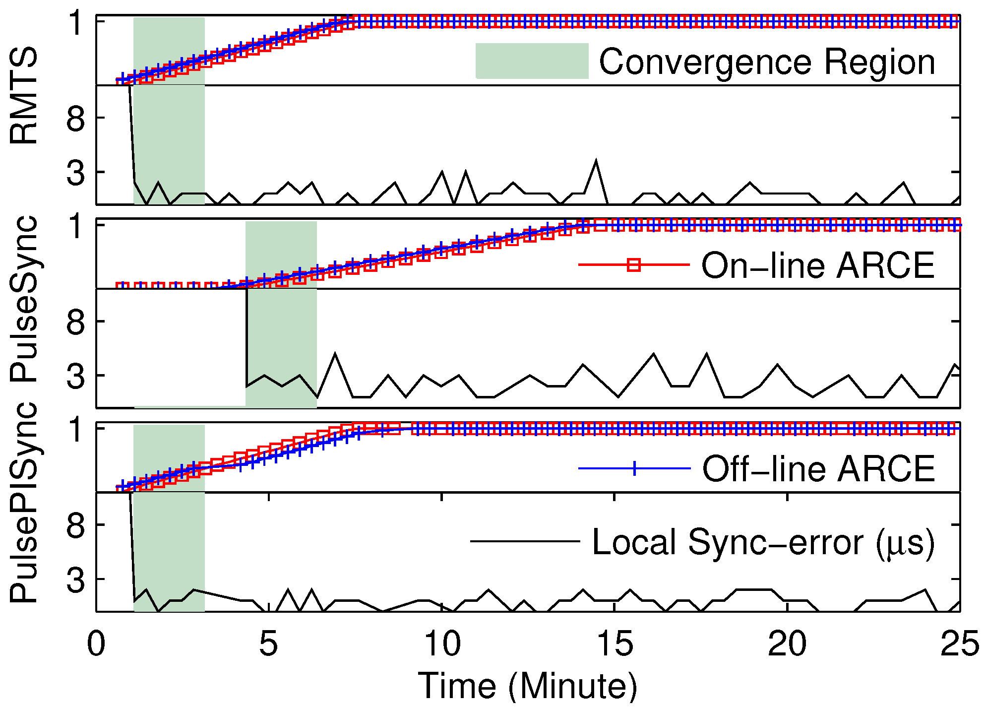
Actual sync error: The instantaneous $E_l$ and $E_g$ of ATS, MACTS, FloodPISync, and RMTS are shown in Figure 2. It is clear that most of the experimental results can be divided into two phases, i.e., the setup and the hold-on. At the setup phase, network-wide time synchronization has not been established; thus, the sync error is unstable and shows a decreasing trend. During the hold-on phase, the sync error is almost stable, and network-wide time synchronization has been achieved.

Therefore, we determine that the time synchronization has locally converged when the local sync error is in the hold-on region. It is clear that the local sync error in the hold-on region is a wide stationary random sequence. Specifically, as shown in

Table 1. The maximum absolute synchronization error and 95% confidence interval (CI). The clock granularity is 1 µs.

Algorithm	Max. Local Sync Error			Max. Global Sync Error
	$\mathit{\mu }$ (µs)	$\mathit{\sigma }$	CI of $\mathit{\mu }$ (µs)	$\mathit{\mu }$ (µs)	$\mathit{\sigma }$	CI (µs)
FCSA	1.61	0.54	1.59∼1.63	3.03	1.26	2.98∼3.08
PulseSync	1.26	0.76	1.22∼1.30	2.50	1.18	2.44∼2.56
FloodPISync	1.49	0.48	1.45∼1.53	2.54	0.87	2.47∼2.61
RMTS	0.99	0.32	0.97∼1.02	1.49	0.56	1.44∼1.53
ATS	2.44	0.54	2.39∼2.49	7.35	1.65	7.19∼7.50
MACTS	2.23	0.45	2.19∼2.24	4.35	1.40	4.24∼4.47

, the mean is constant and the autocorrelation is independent of the start time.

4. Proposed ARCE

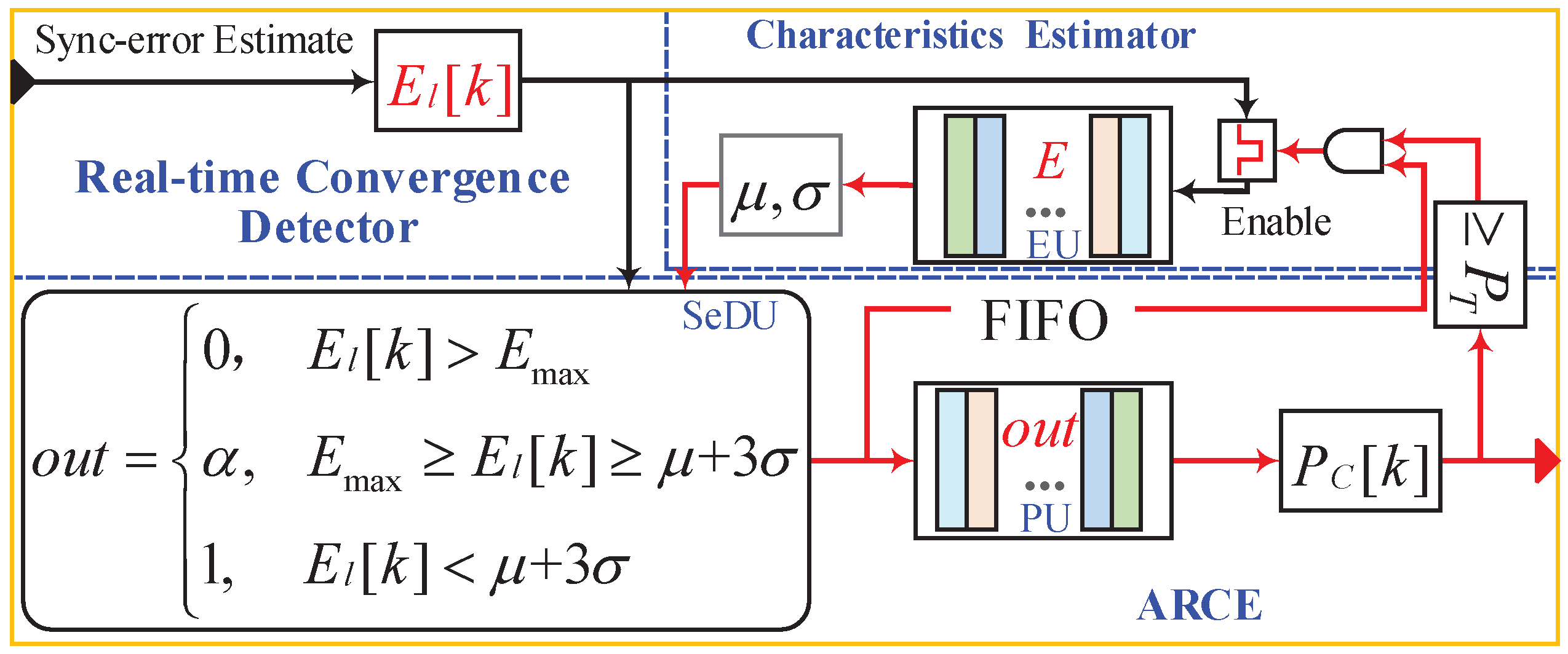
Based on the distribution of the sync error, the proposed ARCE detector is developed and shown in Figure 3, where a sync-error characteristic estimator and a convergence probability estimator are designed for feedback. Considering a real WSN, it is impossible to estimate the global sync error at a local node due to the multi-hop topology of the network. However, it is easy to obtain the local sync-error estimations by using pairs of timestamps that are generated by adjacent (or multi-hop) nodes.

ARCE uses the local sync-error estimate ${\widehat{E}}_l\left[t_k\right]$ as an input parameter; $t_k$ represents the time required for the k-th synchronization, where k is the synchronization count. Thus, it is an approach to detect local convergence. The output of ARCE is a probability estimation, i.e., ${\widehat{P}}_C\left[t_k\right]\in (0,1)$. Using the parameter ${\widehat{P}}_C\left[t_k\right]$, the time synchronization algorithm can estimate the convergence state of the local network in real time.

The sync-error characteristic estimator is a model that estimates sync error. It is driven by the convergence probability. It is employed to calculate the statistical characteristic of sync error, i.e., the mean $\widehat{\mu }$ and standard deviation $\widehat{\sigma }$. The first-in first-out (FIFO) buffer is used to store the convergent sync-error observations, i.e., error-buffer unit (EU). In addition, the convergence probability ${\widehat{P}}_C\left[t_k\right]$ drives the estimator to update the EU. That is, ${\widehat{E}}_l\left[t_k\right]$ will be injected into the EU only if ${\widehat{P}}_C\left[t_k\right]\ge P_T$. Therefore, the sync error in the EU is the observation after which the time synchronization has converged.

The convergence probability estimator is composed of three parts, i.e., a sync-error discrimination unit (SeDu), probability-buffer unit (PU), and ${\widehat{P}}_C\left[t_k\right]$ calculator. The convergence process of local sync error is divided into three phases, i.e., setup, transition, and hold-on. Then, the SeDU is designed as a piece-wise function, and parameter out is the convergence weight for the observation ${\widehat{E}}_l\left[t_k\right]$. In addition, the FIFO PU is employed to store out for its corresponding observation ${\widehat{E}}_l\left[t_k\right]$, and the dynamic array that is used to calculate ${\widehat{P}}_C\left[t_k\right]$ will be filled with 0, $\alpha$, and 1. Here, $\alpha$ represents the cumulative value of single-word convergence; the smaller the $\alpha$, the greater the convergence delay of ARCE, and vice versa.

4.1. Real-Time Local Sync-Error Estimation

According to the existing time synchronization algorithm, the clock parameter estimations and the sync-error estimations are both calculated based on pairs of instantaneous timestamps. For instance, timestamps of $H\left(t\right)$ are used to calculate ${\widehat{\phi }}_i^j$, and timestamps of $L\left(t\right)$ are used to estimate ${\widehat{\theta }}_i^j$. For ease of implementation, relative clock offset estimation ${\widehat{\theta }}_i^j$ is employed to estimate ${\widehat{E}}_l\left[t_k\right]$ in ARCE.

Considering nodes $v_i$ and $v_j(j\in {\mathcal{N}}_i)$, relative clock offset estimation ${\widehat{\theta }}_i^j$ based on the one-way broadcast model is given by

$${\widehat{\theta }}_i^j\left(t\right)=\underset{j\in {\mathcal{N}}_i}{sup}\{L_i\left(t\right)-L_j(t+D)\},$$

(12)

where delay D is assumed to follow a Gaussian exponential distribution. According to the local sync-error model in (6), (12) can be rewritten as

$${\widehat{\theta }}_i^j\left(t\right)\approx \underset{j\in {\mathcal{N}}_i}{sup}\{L_i\left(t\right)-L_j\left(t\right)\}+D=E_l\left(t\right)+D$$

(13)

where $E_l\left(t\right)$ is the sync error for $v_i$ and $v_j$.

Therefore, a local sync-error estimation for nodes $v_i$ and $v_j$ is given by

$${\widehat{E}}_l\left[t_k\right]={\widehat{\theta }}_i^j\left[t_k\right]=L_i\left[t_k\right]-L_j\left[t_k\right],$$

(14)

where $L_i\left[t_k\right]$ and $L_j\left[t_k\right]$ are a pair of timestamps. Note that the estimation error of ${\widehat{E}}_l\left[t_k\right]$ is mainly composed of D, which is equivalent to (10). In addition, it is equivalent to (11) in the time synchronization algorithm based on the two-way message exchange model. The value ${\widehat{\theta }}_i^j\left[t_k\right]$ represents ${\widehat{\theta }}_i^j\left(t\right)$ at time $t_k$.

4.2. Implementation of ARCE Algorithm

According to Figure 3, the pseudo-code of ARCE is presented in Algorithm 1. Parameters $E_{\max }$, $\widehat{\mu }$, $\widehat{\sigma }$, $\alpha$, and $P_T$ are initialized to a non-zero constant; meanwhile, out, ${\widehat{P}}_C$, FIFO EU, and PU are initialized to zero.

Algorithm 1 The pseudo-code of the ARCE algorithm.

˙Initialization:

Set Emax, $\hat{\mathit{\mu }}$, $\hat{\sigma }$, α, and PT

Clear out, ${\widehat{P}}_C$, FIFO EU and PU

˙Upon Receving ${\widehat{E}}_l\left[t_k\right]$:

Calculate (${\widehat{E}}_l\left[t_k\right]$, $\hat{\mathit{\mu }}$, $\hat{\sigma }$, Emax, a) →out

Update FIFO, out →PU

generate PU→ ${\widehat{P}}_C$

˙Upon ${\widehat{P}}_C$ ≥ PT and out > 0:

Update FIFO, ${\widehat{E}}_l\left[t_k\right]$ →EU

Update characteristic parameters, EU→ ($\hat{\mathit{\mu }}$, $\hat{\sigma }$)

Parameter $E_{\max }$ is a threshold for the transition phase of the time synchronization algorithm. Parameter $E_{\max }$ is set based on the experience of the accuracy of the time synchronization algorithm and the granularity of the clock source. For instance, if the accuracy of the time synchronization algorithm is about N ticks of the clock source, then $E_{\max }$ can be set to $m\times N(m>1)$ ticks, e.g., 200 µs. In addition, $E_{\max }$ can be updated in real time by using $\widehat{\mu }$ and $\widehat{\sigma }$, given by

$$E_{\max }=\rho \widehat{\mu }+\beta \widehat{\sigma },$$

(15)

where $\rho >1$ and $\beta >1$. In the following experiments and simulations, $\rho$ and $\beta$ are set to 2 and 3, respectively.

The initial values of parameters $\widehat{\mu }$ and $\widehat{\sigma }$ can be set to be a little greater than the values of the prior experimental results. For instance, according to prior experimental results, shown in Table 1, $\widehat{\mu }$ and $\widehat{\sigma }$ for RMTS can be initialized to 5 µs and 2 µs, respectively. In addition, $P_T\in (0,1)$ and $a\in (0,1)$ are the convergence decision coefficients. Specifically, there is a loose convergence if $P_T\to 0$ or $a\to 1$, and the reliability and stability of $\widehat{\mu }$ and $\widehat{\sigma }$ will decrease, while the convergence decision rate will increase. In contrast, it is a strict convergence if $P_T\to 1$ or $a\to 0$, which leads to an opposite trend of changes in $\widehat{\mu }$ and $\widehat{\sigma }$. Thus, to set appropriate $P_T$ and $\alpha$, the convergence characteristics of the time synchronization algorithm should be considered. For instance, according to the fluctuation of sync error shown in Figure 2, a greater value of $P_T$ is suitable for RMTS, PulseSync, and PulsePISync, while a smaller value is suitable for ATS, FCSA, and MACTS.

The weight parameter out is calculated based on the piece-wise function that is indicated in Figure 3 (Algorithm 1, Line 1). By using the updated weight array PU, the ${\widehat{P}}_C$ is expressed as

$${\widehat{P}}_C={\displaystyle \frac{\sum PU}{L_P}},$$

(16)

where $L_P$ is the depth of the FIFO PU. In addition, the depths of the PU and EU are related to the convergence rate and the smoothness of ${\widehat{P}}_C$, respectively. A smaller depth of the PU leads to faster convergence for ${\widehat{P}}_C$, and a greater depth of the EU leads to smooth ${\widehat{P}}_C$. Thus, the FIFO can be used to balance the rate and reliability of convergence decisions in ARCE by changing the depth.

5. Performance Evaluation

To evaluate the proposed ARCE, a prototype system is built with 9 Synchronous Sensing Wireless Sensor (SSWS) nodes that have been described in detail in [21,27]. Specifically, a line topology testbed is used to run ARCE on flooding time synchronization algorithms, e.g., FTSP, FCSA, PulseSync, FloodPISync, PulsePISync, and RMTS; one testbed of grid ($3\times 3$) is employed to evaluate ARCE on average consensus approaches, e.g., ATS and MACTS. In addition, the employed sync-error measurement is similar to the one [17,18,19,21,27,33] used, which has been discussed in [21,33].

According to the existing study, a threshold is employed to find the convergence time of the synchronization error [18,24,27], while no common method to detect the convergence state has been proposed. To calculate the estimation error, experiments are designed for off-line ARCE and on-line ARCE, respectively.

• Off-line ARCE, in which the input of ARCE (${\widehat{E}}_l$) is the measuring results for synchronization error, and the results for ARCE are calculated off-line using ${\widehat{E}}_l$, i.e., $T_{\mathrm{RCE}}\left({\widehat{E}}_l\left[t_k\right]\right)$.
• On-line ARCE, in which the proposed ARCE is embedded into the employed time synchronization algorithms, and the clock offset estimation $\widehat{\theta }$ in (13) is employed as input. The actual experimental results are calculated on-line by using $\widehat{\theta }$, i.e., $T_{\mathrm{RCE}}\left({\widehat{\theta }}_i^j\left[t_k\right]\right)$. Therefore, the estimation error becomes

  $$E_{\mathrm{RCE}}=T_{\mathrm{RCE}}-T_C,$$

  (17)

  where $T_C$ is calculated using (8), and the threshold $E_{Th}$ is set as 20 (µs) for the following experiments.

5.1. Experimental Results

Table 2. Parameter settings for experiments with ARCE.

Parameter	${\mathit{P}}_{\mathit{T}}$	$\mathit{\alpha }$	${\mathit{L}}_{\mathit{P}}$	${\mathit{L}}_{\mathit{E}}$	${\mathit{E}}_{\mathbf{max}}$ (µs)	$\widehat{\mathit{\mu }}$ (µs)	$\widehat{\mathit{\sigma }}$
Value	0.9	0.5	20	10	200	30	1

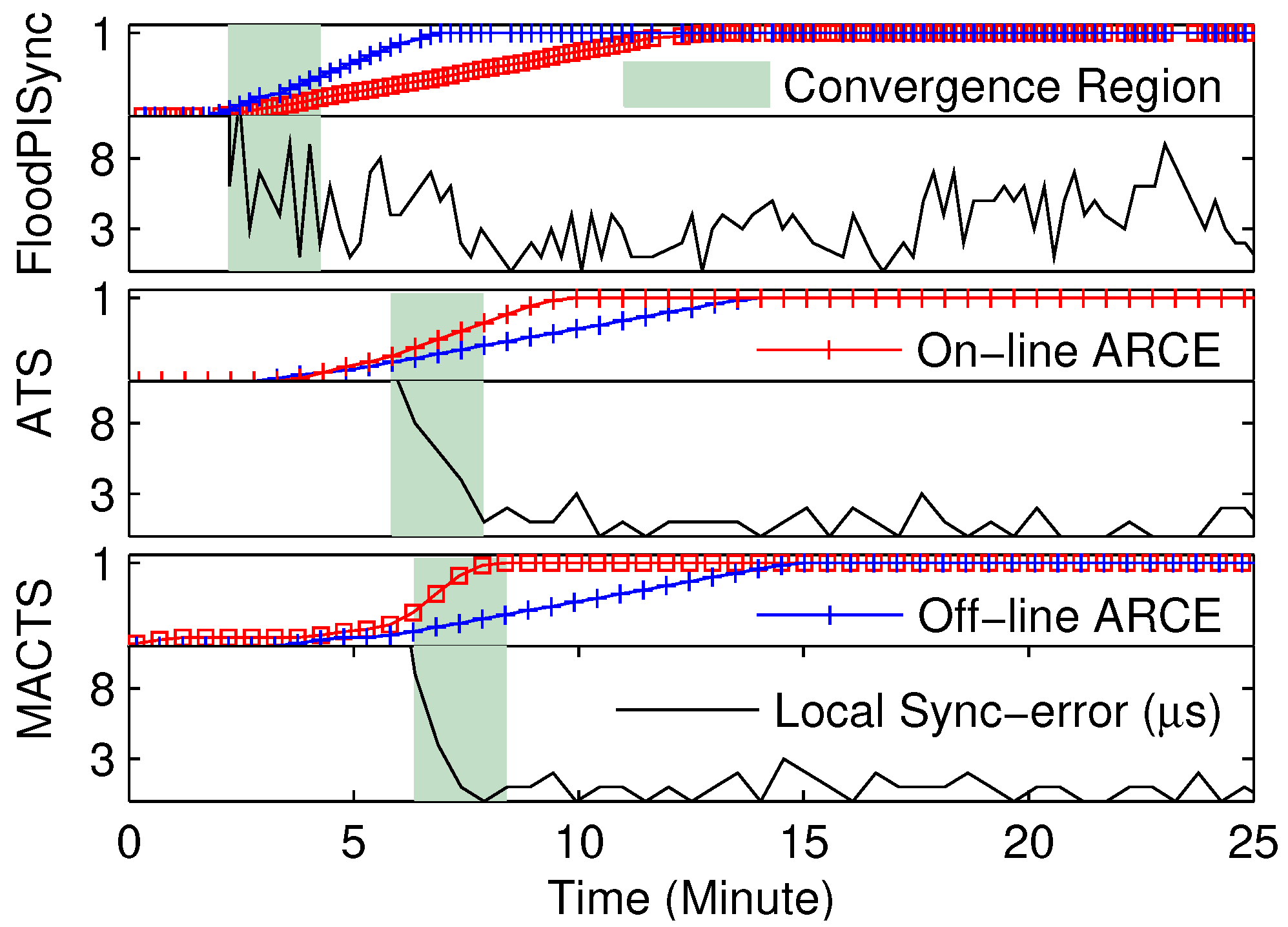
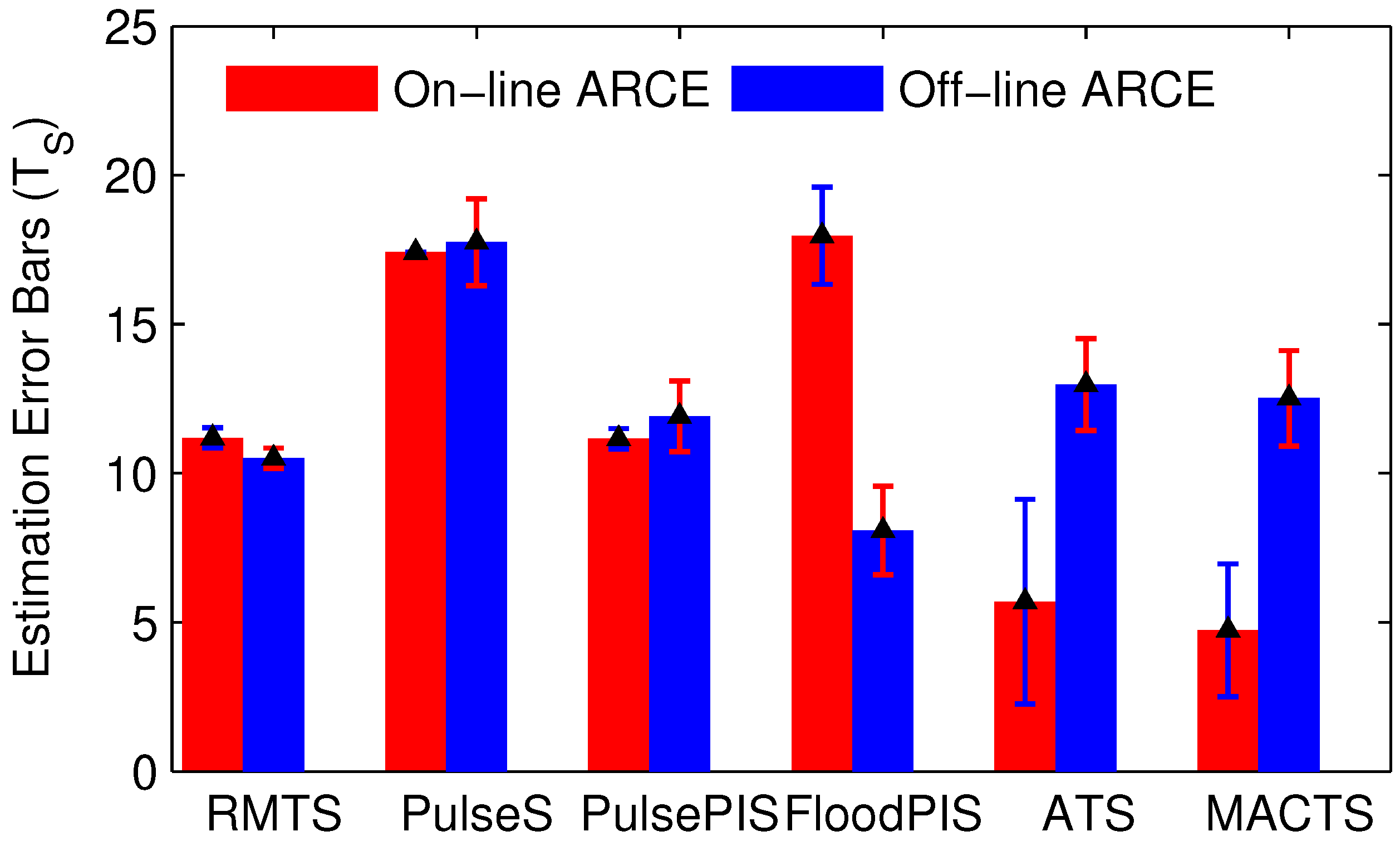
summarizes the default parameter settings. The parameter $E_{\max }$ is updated by (15). The experimental results are illustrated in Figure 4 and Figure 5. Note that RMTS, PulseSync, and PulsePISync are rapid-flooding time synchronization algorithms. In these protocols, all testbed nodes run the synchronization operation at almost the same moment. Thus, they are synchronous time synchronization approaches. However, slow-flooding methods, such as floodPISync, and average consensus methods, such as ATS and MACTS, use an asynchronous approach, where a node runs the synchronization operation based on local time. The ${\widehat{P}}_C$ values of on-line and off-line ARCE are highly similar in the synchronous approach and are obviously inconsistent in the asynchronous method.

Considering the flooding approaches, a comparison between synchronous and asynchronous has been discussed carefully in [21,22]. The average consensus approaches employ iteration to forward the time information among multi-hop nodes. Hence, the main challenge for an asynchronous method is that the time information error will increase continuously due to the forward wait time and the clock drift.

In addition, the error bars in Figure 6 show that the asynchronous method indicates a smaller standard deviation than the synchronous one. Basically, by using the synchronous method, time synchronization can be established for all nodes almost at the same moment, and the global synchronization and local synchronization almost converge simultaneously. However, considering the asynchronous algorithms, there are slight differences in the time synchronization convergence time among nodes.

Furthermore, the experimental results of on-line and off-line ARCE are very close to each other. The convergence latency for on-line and off-line ARCE is about 1, 1, 1, 20, 15, and 15 synchronization intervals in RMTS, PulseSync, PulsePISync, FloodPISync, ATS, and MACTS, respectively. Thus, using $\widehat{\theta }$ as input is reasonable for on-line ARCE. The maximal convergence estimation error is about 21 synchronization intervals in FloodPISync. Therefore, the proposed ARCE is realizable and reliable for the comparison of time synchronization algorithms to detect local synchronization convergence.

However, for the distributed and asynchronous time synchronization algorithms, e.g., ATS and MACTS, the convergence time is different between local synchronization and global synchronization. In addition, such differences may increase when the time synchronization algorithm is deployed in more complex networks. Thus, if the presented ARCE is considered to detect the global synchronization convergence of an asynchronous approach, the latency between local and global synchronization convergence should be compensated for.

5.2. When out of Sync

Considering dynamic wireless networks, serious synchronization skew may be caused by changes in topology and environment, e.g., new node joints or communication interference. Specifically, local synchronization error will propagate among multi-hop nodes or even network-wide. Thus, once a large synchronization error is generated at a local node, it will result in a lack of synchronization at that local network. To avoid the spread of synchronization error, it requires neighbors of the node to detect the out-of-synchronization situation.

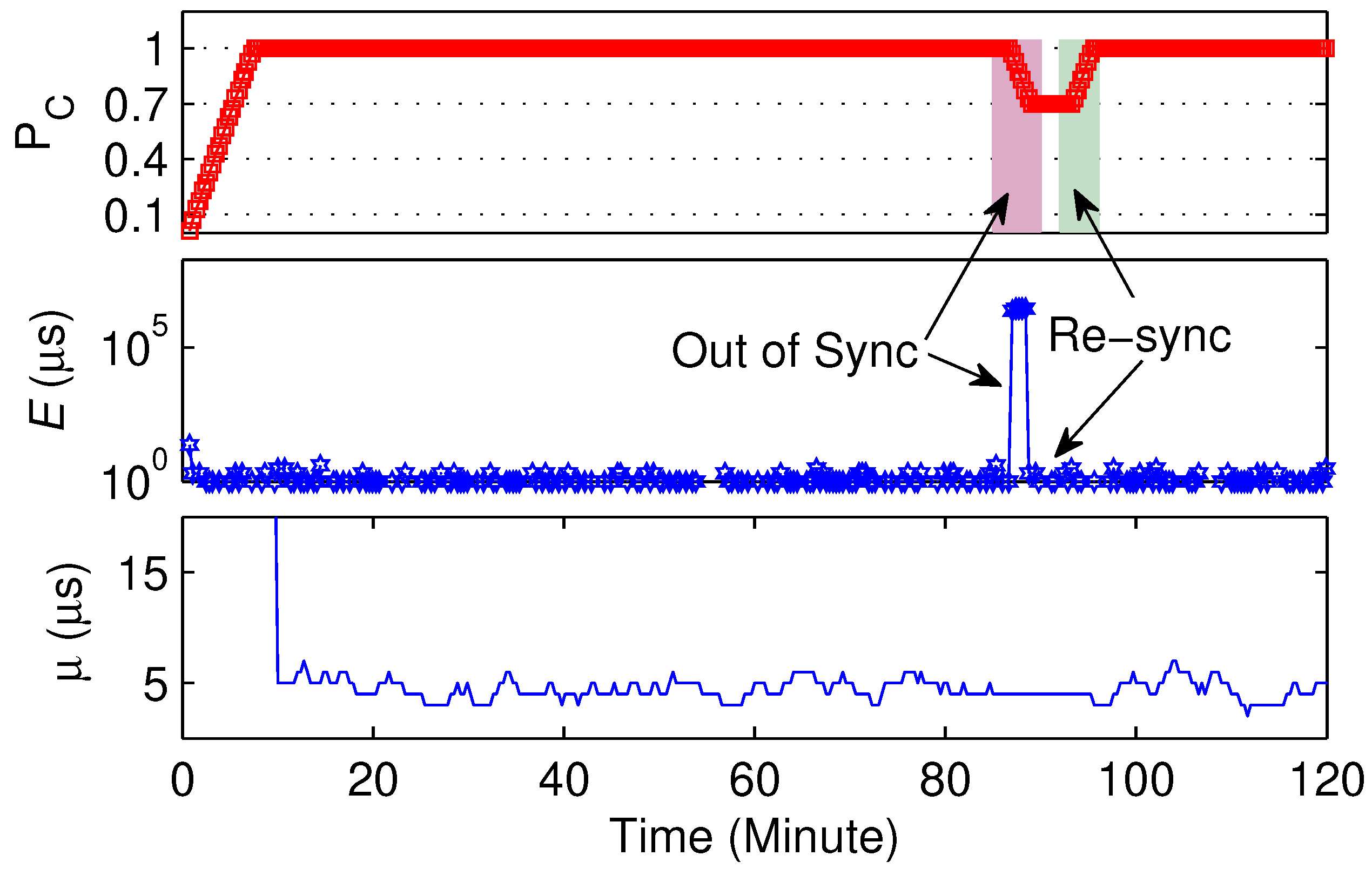
We evaluate the on-line ARCE based on RMTS and restart a node ($v_i$) at 87 min. The experimental results in Figure 7 are calculated with $v_j(j\in {\mathcal{N}}_i)$. As shown in the middle panel of Figure 7, the $E_l$ suddenly increases at the moment that $v_i$ restarts, then the $P_C$ of $v_j$ is reduced and indicates the out-of-synchronization situation (upper panel of Figure 7). In addition, ARCE also indicates the re-synchronization of $v_i$. The lower panel of Figure 7 shows the $\widehat{\mu }$ of local synchronization error, where the samples among the region in which $v_i$ is out of synchronization are removed from the FIFO EU; thus, $\widehat{\mu }$ is a fixed value in that region.

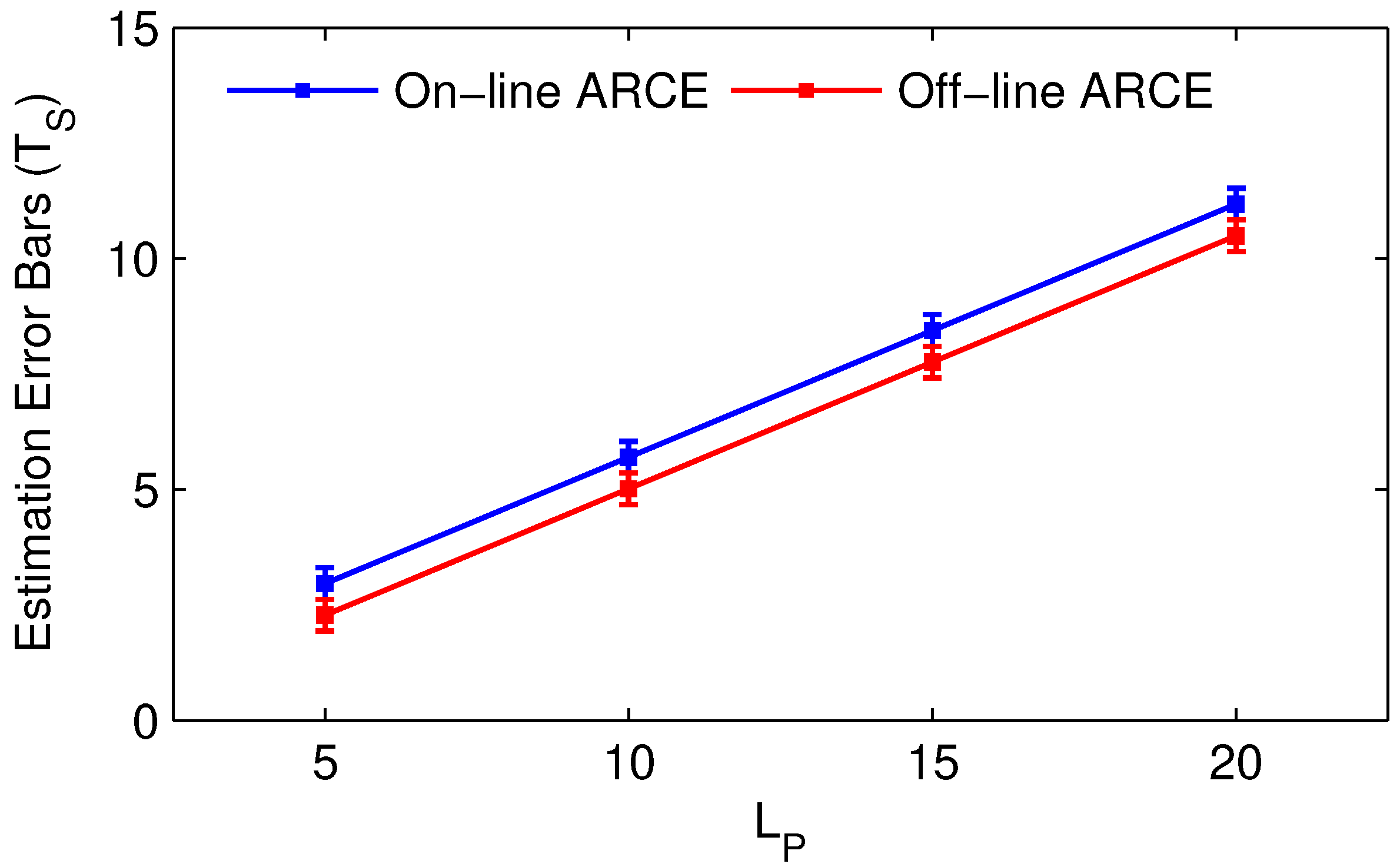
5.3. Discussion on $L_P$

According to the above-mentioned experimental results, we observe that the convergence estimation error is highly related to the width of the observation window, i.e., the length of FIFO PU $L_P$. Therefore, we evaluate ARCE based on RMTS and set the $L_P$ as 5, 10, 15, and 20, separately. From the experimental results in Figure 8, it is clear that the larger $L_p$ results in higher $E_{\mathrm{RCE}}$. Hence, (a) a smaller value of $L_P$ can be used to achieve highly sensitive convergence detection and (b) a larger $L_P$ can be used to design smoother convergence detection.

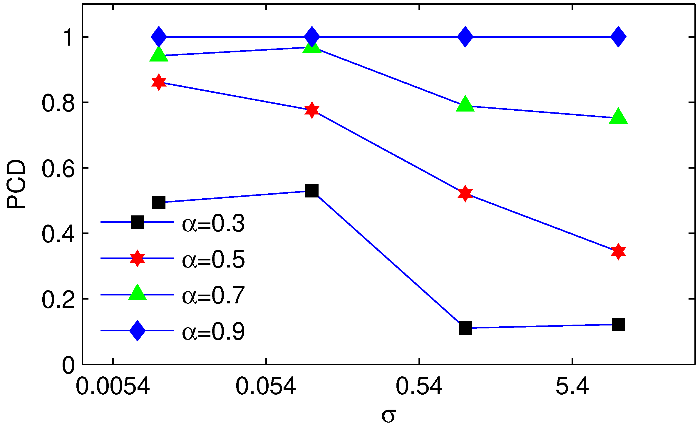
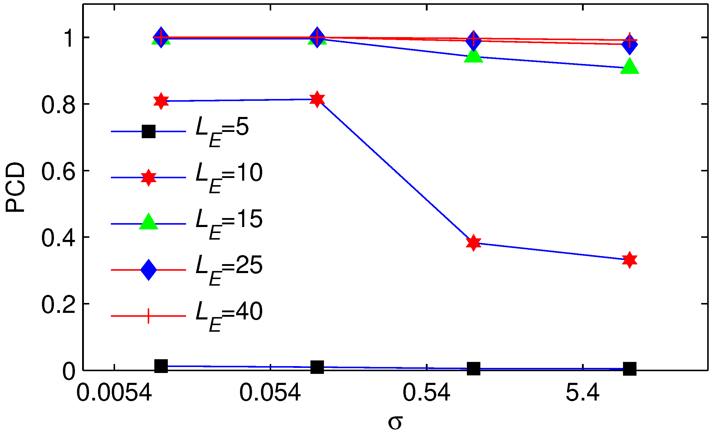
5.4. Discussion on $\alpha$ and $L_E$

To find the relationship between the parameters $L_E,a$, and the performance of ARCE, a simulation is built based on MACTS. Definition of probability of convergence detection (PCD): Considering the time synchronization as totally convergent, the PCD is the probability of ${\widehat{P}}_C>P_T$. Hence, the PCD is used to describe the possibility of ARCE successfully detecting the convergence status. We evaluate ARCE under different delay levels, where the delay is Gaussian with mean 3.3 µs with standard deviations $\sigma$ of 0.0054, 0.054, 0.54, and 5.4, separately. The experimental results for $\alpha$ and $L_E$ are shown in Figure 9 and Figure 10, respectively. We observe that a larger $\alpha$ or a deeper FIFO EU leads to the ARCE being more robust; as a result, ARCE achieves a higher PCD. Therefore, by adjusting either parameter $\alpha$ or $L_E$, ARCE can be made more stable and better handle the change in random delay.

6. Implications

Recently, self-adaptability has been considered an important feature of time synchronization algorithms. For instance, PISync uses a proportional–integral controller to compensate for the relative clock rate, and MACTS employs a multi-hop controller to reduce multi-hop communication. However, it is important and difficult to set an appropriate threshold for these controllers, e.g., the maximum synchronization error $e_{\max }$ in the adaptation algorithm of PISync and the maximum local synchronization error $\xi$ in MACTS.

Specifically, as we discussed in detail in [21,22,27,34], the synchronization error highly depends on the following factors:

(1)

The accuracy of the clock parameter estimations. The relative clock offset estimation error is a major portion of the synchronization error of a time synchronization algorithm in the setup region. In addition, the relative clock rate estimation error is an important reason for the clock skew of the algorithm in the hold-on region.

(2)

The random package variable delay. As is well known, delay poses major challenges to accurate clock parameter estimation, and suppression of transmission delay is one of the key techniques to improve the accuracy of time synchronization in existing algorithms.

(3)

The topology of wireless networks. The diameter and shape of topology severely limit the actual accuracy of time synchronization algorithms, and diameter is a major factor in the bound of time synchronization errors [35].

Therefore, both increases in delay and changes in topology will cause changes in actual synchronization error. As a result, by using the frequency difference ($\Delta f_{\max }$) between the upper and lower bounds of the oscillators to configure $e_{\max }$ in PISync, if the actual synchronization error is always larger than $e_{\max }$, the time synchronization cannot converge. Considering MACTS, a constant $\xi$ is configured based on prior experimental results; thus, the changes in actual delay may cause convergence detection failure.

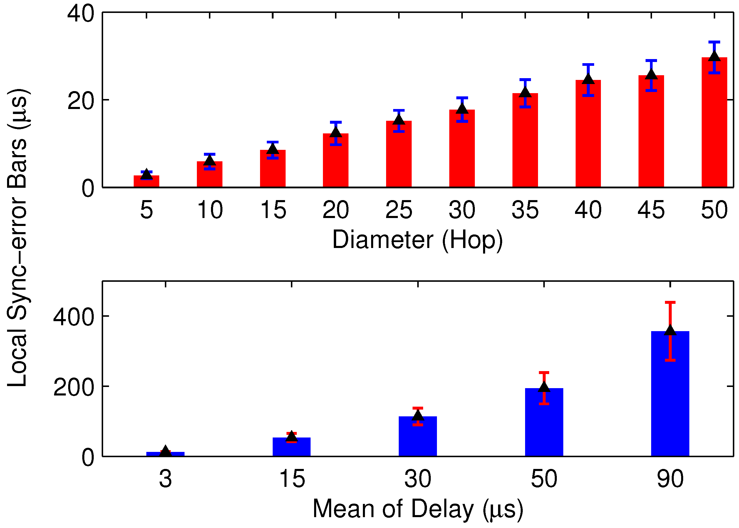
6.1. Challenges in MACTS

In this part, a simulation model is built for MACTS. The clock frequency offset is a random variable in the range of $\pm 40$ parts per million, and the delay is a random Gaussian variable. We evaluate the changes in synchronization error based on a line topology network, and the simulation of local synchronization is shown in Figure 11. It is clear that both an increase in the network diameter and delay will significantly increase local synchronization error. Thus, for a randomly deployed wireless network, the unpredictable network topology and delay pose challenges to setting a suitable $\xi$ for MACTS. Specifically, a larger value of $\xi$ may lead to slow convergence, while a smaller one may cause failure of the multi-hop controller.

6.2. ARCE-Based MACTS

The presented ARCE is considered to improve the MACTS, which is shown in Figure 12 and is named ARCE-MACTS. The main difference between MACTS and ARCE-MACTS is the multi-hop controller, where ARCE is used to replace the threshold detection. The output of ARCE is the convergence status of local synchronization error, and the controller reduces or increases the multi-hop number H based on the output.

Simulations of ARCE-MACTS and MACTS are developed, where a $10\times 10$ grid network is employed, and H is initialized as 3. The parameters are set as $a=0.3$, $P_T=0.9$, $L_P=20$, and $L_E=40$. The initial values of parameters $\widehat{\mu }$ and $\widehat{\sigma }$ are 450 (µs) and 80, respectively. The parameter $E_{\max }$ is calculated using (15). The means of Gaussian delay are set as 3, 15, 30, 50, and 90 (µs), and the corresponding standard deviations are set as 0.005, 0.05, 0.5, 5, and 15, respectively. The parameter $\xi$ of MACTS is set as 20 (µs), which was set as 5 (µs) in the above experiments with MACTS.

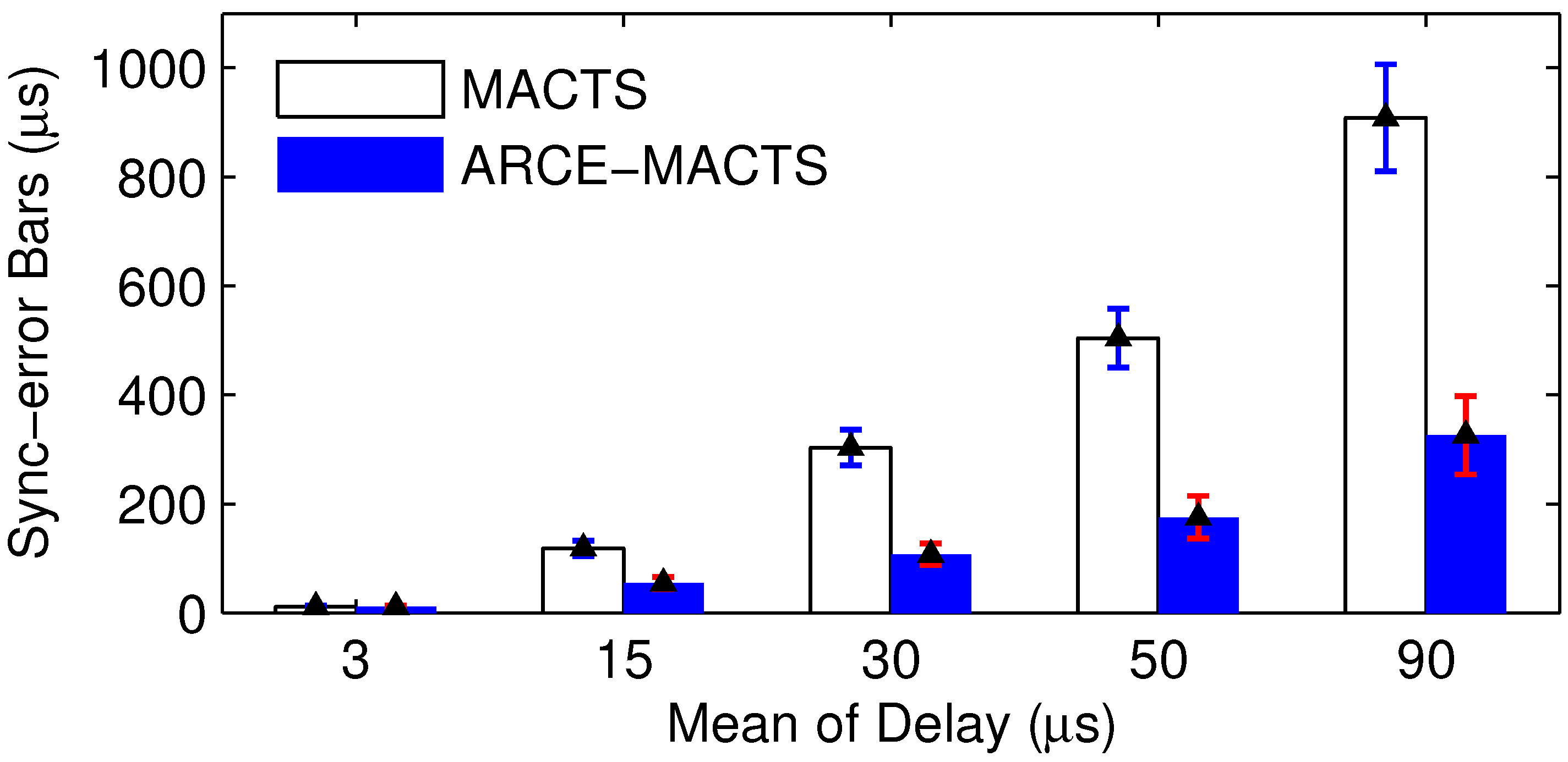
The convergence detection time (CDT) is summarized in

Table 3. The convergence detection time (CDT) of local sync error.

Mean of Delay (µs)	CDT MACTS (Min)	CDT ARCE-MACTS (Min)
3	18	15
15	False	15
30	False	15
50	False	15
90	False	15

, and the maximal global synchronization error bars of simulations are shown in Figure 13. The results show that MACTS fails to detect the convergence time at a larger delay level. From the results, we see that the multi-hop number H is always equal to 3 and MACTS never converges to one-hop communication. In addition, the global synchronization error of MACTS is significantly larger than that of ARCE-MACTS. Note that the drawbacks of multi-hop communications for time synchronization, e.g., increased communication collision, by-hop error accumulation, and energy consumption, are studied in [21,27].

6.3. Discussion

However, the synchronization error highly depends on the hardware of the implementation, e.g., the granularity of the clock system and the computational accuracy of the processor. In our latest work, we designed a testbed based on FGPA and CC2538, in which the clock system was designed based on FPGA, and the clock granularity was set to 10 ns, i.e., the clock frequency was 100 MHz. Moreover, we extended the GNSS to synchronize mutually independent WSN systems. In this testbed, a reference node of the local network synchronizes itself to the GNSS, and then the network nodes synchronize to this reference. Commonly, the synchronization error of reference nodes to the GNSS is as low as 100 ns; therefore, the synchronization error for different WSNs is much lower. In our existing experimental results, the averaging synchronization error (or synchronization accuracy) for two different WSNs is as low as 0.34 µs, and the average synchronization error (or synchronization accuracy) for the reference (host node) and its neighbor (slave node) is as low as 0.05 µs.

In the current ARCE method, the focus is primarily on a single synchronization source. However, in real-world applications, especially in distributed systems, multiple data sinks or nodes with varying computational and communication capabilities may exist. The ARCE method can be adapted to address these challenges. In multi-sink networks, the method could be extended by enhancing the synchronization algorithm to minimize the time synchronization errors between sinks, ensuring consistency across the entire network. Additionally, in heterogeneous networks, the synchronization strategy can be adjusted based on the capabilities of the nodes. Higher-precision synchronization could be applied to nodes with stronger computational capabilities, while simplified synchronization approaches could be used for nodes with lower capabilities. In this way, the ARCE method can maintain high synchronization accuracy and network efficiency across diverse network environments.

In practice, the ARCE method could also have significant applications in real-world scenarios that require precise synchronization, such as in distributed energy systems like solar panel monitoring. For example, in our experimental setup, we extended the GNSS to synchronize the WSNs, where the synchronization error for reference nodes to the GNSS was as low as 100 ns. With the ARCE method, such high-precision synchronization could ensure synchronized fault detection across multiple devices, thus improving the overall efficiency and reliability of energy management systems. This can be particularly valuable in applications such as distributed solar panel monitoring, where precise synchronization is crucial for detecting and responding to faults across a large, geographically distributed network.

7. Conclusions

In this paper, we have proposed ARCE to detect the convergence status of a time synchronization algorithm in real time, which can be used to develop an adaptive time synchronization algorithm. By using a sync-error discrimination unit and a sync-error characteristic estimator, ARCE generates the convergence probability and the statistical characteristic of synchronization error, respectively. The output of the characteristic estimator is fed back to update the detection condition of synchronization convergence. As a result, ARCE can adapt to changes in delay and be easily deployed without any prior experimental results.

Evaluations are designed for ARCE based on flooding and average consensus time synchronization algorithms, separately, where both synchronous and asynchronous time synchronization approaches are employed. Additionally, the parameter settings and the implications of ARCE are discussed in detail. According to the experimental results and simulations, ARCE can effectively detect the convergence state for all the comparisons. Therefore, ARCE can be used to develop an adaptive time synchronization protocol, which could be robust and scalable for a large-scale and randomly deployed wireless network.