Article

High-Resolution Building Indicator Mapping Using Airborne LiDAR Data

1
School of Surveying and Built Environment, University of Southern Queensland, Springfield Campus, Springfield, QLD 4300, Australia
2
Institute of Geodesy and Civil Engineering, Faculty of Geoengineering, University of Warmia and Mazury in Olsztyn, 10-719 Olsztyn, Poland
3
School of Civil Engineering, Purdue University, West Lafayette, IN 47907, USA
*
Author to whom correspondence should be addressed.
Electronics 2025, 14(9), 1821; https://doi.org/10.3390/electronics14091821
Submission received: 25 February 2025 / Revised: 24 April 2025 / Accepted: 27 April 2025 / Published: 29 April 2025
(This article belongs to the Special Issue Point Cloud Data Processing and Applications)

Abstract

:
Urban indicators established in spatial development plans should ensure the preservation of spatial order when introducing new construction investments. They should also harmonize with the existing urban structure and even modernize it toward sustainable development. When determining these indicators, the surrounding space is analyzed. Conventionally, building indicators in the existing space are determined based on available documents, which usually comprise 2D spatial data such as large-scale maps or cadastral maps. This study aims to investigate the method of calculating building indicators using 3D urban building models that will be created from airborne Light Detection and Ranging (LiDAR) measurements. In the discussion of the results, indicators calculated based on LiDAR data are compared with the ones calculated from 2D cadastral data. The calculated 3D indicators correlate with the classically calculated indicators. The accuracy of the computed building area, volume, and other indicators depends on the LiDAR point cloud density and accuracy. The indicators calculated from the 3D data align with the new trends in defining Building Morphology Indicators (BMIs).

1. Introduction

In the era of creating digital twins of the real world, we should more frequently utilize available 3D spatial data in daily tasks to support the development of smart cities and sustainable urban growth. Three-dimensional (3D) data enable the calculation of urban [1,2,3], environmental [4], ecological [5], social, economic, and institutional indicators [6,7], as well as of programming indicators [8]. In urban spaces, recommended transport indicators (ISO) [9], accessibility indicators for various urban services [10], public green spaces, public utility facilities, and many others [11,12] are assessed. Multiple analyses are also conducted, aimed at identifying specific areas in urban spaces, such as heat islands [13].
In urban planning and spatial development, to better understand the environment and built structures, solutions based on 3D city models should be widely implemented [12,14,15]. This is essential when making decisions regarding new investments [16,17] based on necessary indicators that ensure not only sustainable development but also the preservation of landscape values, such as those related to shading in urban spaces [9], visibility of the sky [18], and the perception of buildings by people [19].
It is recommended that the construction of virtual cities be conducted using the City Geography Markup Language (CityGML3.0) standard [20,21]. This is recommended by the Open Geospatial Consortium (OGC), the standard building organization that organizes data models and forms of their exchange [22,23]. Buildings are the basis of city 3D models. Vector models of buildings linked to semantic data are required. The CityGML3.0 standard defines the Levels of Detail (LODs) of building models from LOD0 to LOD 4. In [24], an extension is proposed that contains a total of 16 subdivided LODs, which are presented in Figure 1.

1.1. Cadastral Data in Spatial Planning

Spatial planning uses available spatial data at different levels of detail: 2D and 3D. For the calculation of urban indicators of built-up areas, 2D cadastral data with the detail of building models at the LOD0 level are often used [25,26]. Cadastral attribute data, indicating the number of stories, allow models to be generated at the LOD1 level (Figure 1) [24,26]. The development of 3D technology has created new possibilities for the automatic generation of urban space development. Despite this, the creation of spatial planning is performed by traditional methods using 2D data and the calculation of indicators is based on this data [25,27,28].

1.2. Three-Dimensional (3D) Data in Spatial Planning

The systems created based on the CityGML standard are dedicated to various users, including architects creating spatial development plans for cities based on 3D data [29]. Available cloud platforms for spatial visualization and analysis, such as Google Earth Studio, Urban Sim, Unreal Engine, and many others, enable 3D space visualization and advanced analyses. Both commercial and open GIS systems are rapidly advancing their 3D analysis tools. The availability of data and modern tools has driven the development of local solutions for presenting and analyzing 2D and 3D data. This is achievable, provided we have 3D vector data and appropriate processing algorithms. Digital data sets, such as those from LiDAR, offer a new perspective on space by enabling the automatic generation of 3D object–vector representations and analyses of urban spaces. An example of this is the capability to create digital models of individual buildings [30,31,32,33,34] and to generate 3D models of entire cities at the LOD2 level [34,35,36]. These proposed solutions are becoming increasingly advanced [37,38,39,40,41,42] through the integration of LiDAR data with remote sensing datasets and the use of machine learning and deep learning techniques [43,44,45].
In the process of automatic model generation and building indicator calculation, there are problems related to poor point cloud quality [46], the density of the point cloud, classification of the point cloud into thematic subsets, segmentation of the point cloud [31], and the incomplete covering of building roofs and walls [47]. To improve the quality of the LiDAR point cloud, additional activities are undertaken through a two-step registration method with trajectory correction [46] by the internal matching of scan blocks in combination with inertial measurements and Global Navigation Satellite System (GNSS) measurements [48].

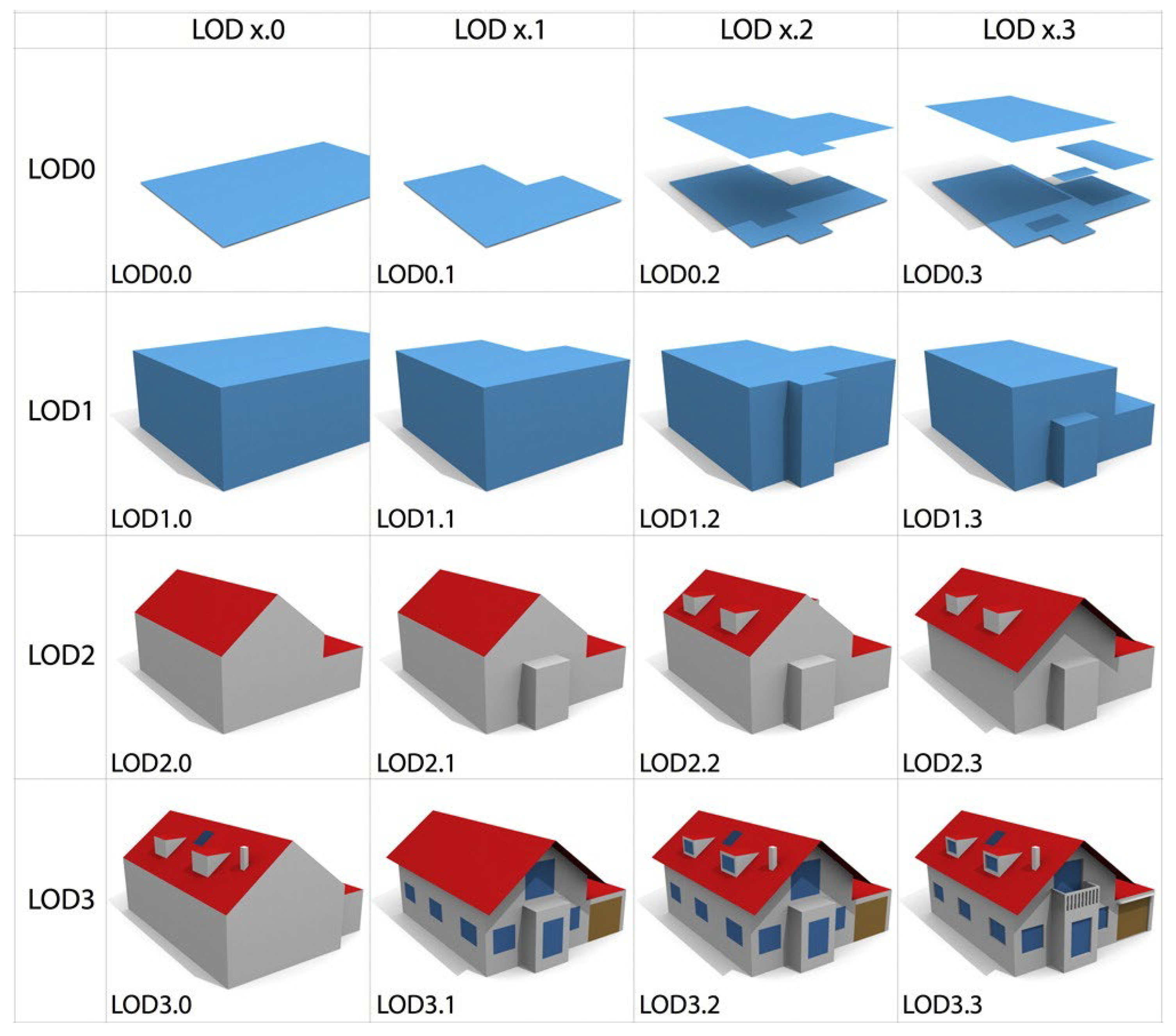
1.3. Quality of 3D Models

Despite increasingly better LiDAR datasets and algorithms for modeling buildings, there are irregularities in the generated contours of buildings and holes in the roof surfaces of buildings [49]. The presented building models are in 2.5D mesh [50] as shells of triangles, called triangles of the building envelope and a mash of triangles [35,51]. These models allow us not only to visualize building models but also to perform analyses related to the shadow estimation of a building’s thermal load [35]. When modeling buildings, there are still problems with the precise mapping of roofs due to the complexity of the slope and the existence of chimneys. The original solution was demonstrated by analyzing elevation jumps at adjacent points of the LiDAR cloud. From the detected subsets of points without height jumps, roof slope fragments are generated [52]. Based on the built roof slopes in the form of 3D planes, a model of the building body is generated at the LOD2 level. They are pulled down from the roof shells and placed on the ground based on the selected height point. The emerging models present buildings without eaves. The size of the roof affects the size of the building mass model. The generated building can be larger than the real one due to the size of the eaves. As we have cadastral outlines of buildings, we usually create models at the LOD1 level. These contours are used for automatic modeling at the LOD2 level based on LiDAR data. This time, the size of the building mass model depends on the outline of the building.
In addition to algorithms for modeling entire cities’ buildings, there are also algorithms available for the automatic creation of urban greenery models, including the generation of individual tree models, green complexes, and the calculation of biomass in biologically active areas [53,54,55,56,57,58] The use of deep learning methods for 3D object recognition and vectorization of other urban space elements will, in the future, enable the widespread use of 3D, and even 4D, digital data for monitoring urban spaces and for calculating indicators that better describe spatial structures using existing [20,44,53,54,59] and new parameters [60].

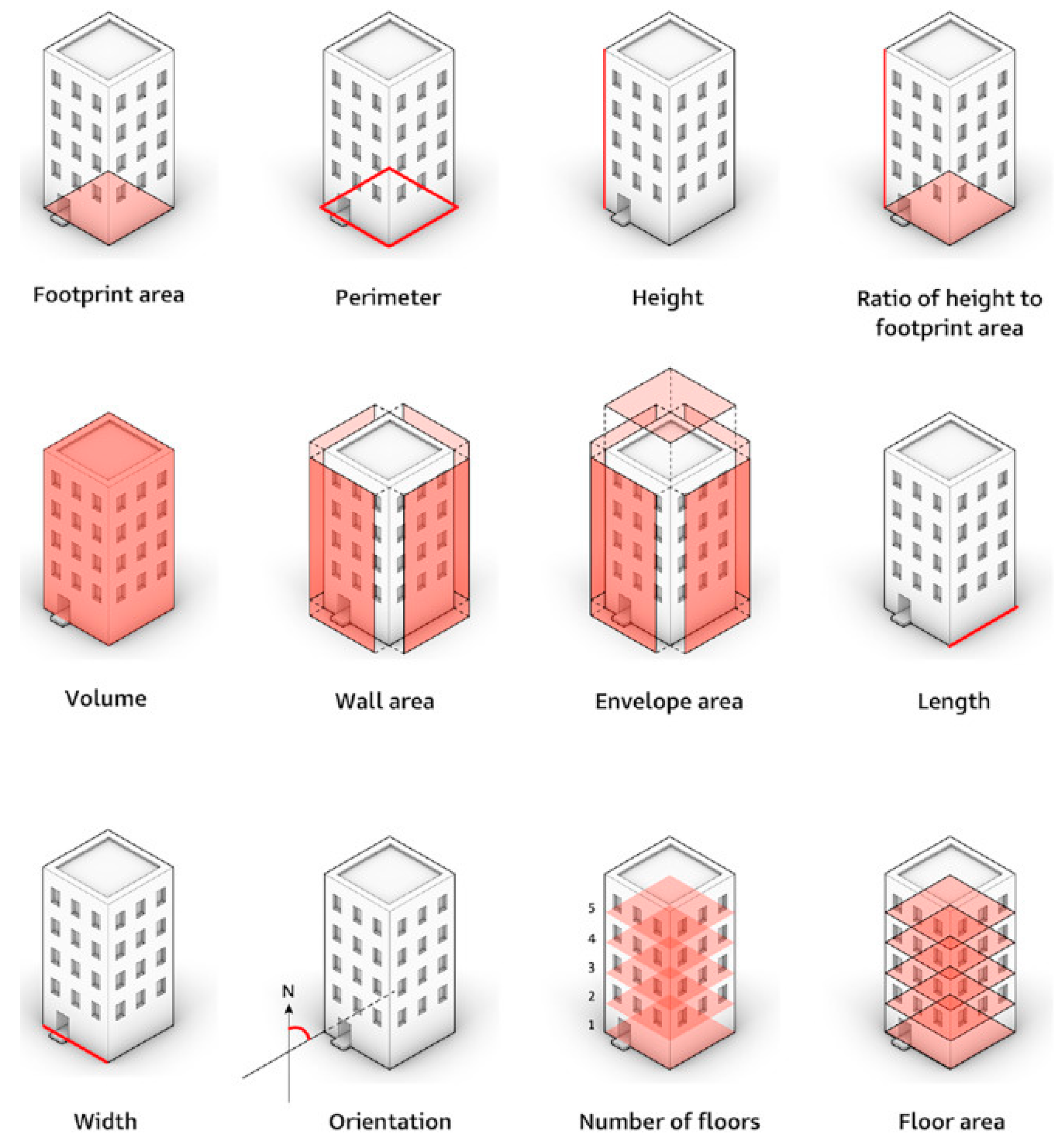
1.4. Three-Dimensional (3D) Urban Space Indicators

Urban areas, both existing and planned, are described in urban planning using indicators that define land use and building parameters [2,61]. These indicators include, among others, the building height, maximum and minimum number of floors, building coverage, and floor area ratio. Other indicators relate to the distance between buildings, the number of parking spaces, recreational areas, and biologically active areas [20]. The methods for calculating these indicators are widely known and documented in standards and local legal documents [62,63] primarily related to spatial planning. Currently, the calculation of indicator values for existing urban areas is based on data from cadastral and topographic maps. The set of indicators in local spatial development plans (MPZP) for areas designated for development are the result of separate analyses of urban spaces based on large-scale 2D maps and other data sets from thematic portals and remote sensing results, such as LiDAR, orthophotos, street views [64], and many others.
New solutions [65,66] are being promoted [67] that introduce global Building Morphology Indicators (BMIs) [60] (Figure 2). Such indicators should be obtained from Building Information Modeling (BIM). In the absence of these, algorithms should be created to obtain them from alternative data.
The presented independent building indicators are used to calculate the development indicators for planning areas (parcel). One of them is the building intensity index. The calculations of this index are based on the sum of the area of all the stories in the building (Floor area; Figure 2) [25,27,63]. In practice, the cadastral area of buildings is used to calculate the sum of the area of all the floors in the buildings. We multiply two numbers: the cadastral area (surface of the model on LOD0) and the number of stories [25,27,63]. Story heights and types of roofing are not included in the 2D cadastral data. Figure 3 shows a 3D visualization of a fragment of a housing estate with different LOD details. Figure 3b,c do not adequately show 3D building models according to their size. The models were created using the cadastral database, the height from LiDAR data (Figure 3b), and the number of stories and the assumed story height (Figure 3c). However, the building intensity index should take into account 3D buildings in LOD3 models (Figure 3a), which are becoming increasingly available. They can also be largely calculated based on a cloud of LiDAR points imaging buildings. This can be expected to be widely adopted when a 3D cadaster is implemented [68,69].
The data presented in Figure 3 show how different 3D models of buildings can be depending on the data adopted and the method of their generation. In the absence of 3D models at the LOD2 level, LiDAR data are a reliable source for detailed research related to planning indicators.
Figure 3 shows only typical simple buildings in a housing estate. Contemporary buildings in urban centers cannot be reliably visualized on the basis of cadastral data. The ground floors of buildings do not coincide with the vertical projection of building blocks, and, in addition, they have numerous superstructures, overhangs, passages or decorative elements, which are often not recorded in the 2D cadaster. Mass-market digital solutions related to Building Information Modeling (BIM) will allow for the creation of 3D models of new buildings in the future. Existing buildings must be modeled on LiDAR measurement data. Already today, technologies based on LiDAR data allow for the precise mapping of urban space. The development of techniques of classification of the LiDAR measurement set, the extraction of subsets describing individual field objects, and their automatic modeling mean that, in the future, we will be able to achieve better and better precision in the created 3D models of buildings and cities.
Finally, it is necessary to highlight the relationship between BIM (airborne, mobile terrestrial, static, and Simultaneous Localization and Mapping (SLAM) laser scanning) and building indicators. One building can have two BIM models: design BIM, which is provided by the building designer before constructing the building, and as-built BIM. However, the basic of any BIM should be a real 3D model outside and inside the building. Old buildings do not have design BIM, but it is possible to construct as-built BIM where both terrestrial (for inside building and facades) and airborne (for the building roof) LiDAR data are the main data sources for this purpose. When the BIM model or updated cadastral maps are available for all city buildings, the building indicators can be calculated automatically. Unfortunately, in general, BIM models are not available for most city buildings and cadastral maps may need updating. Indeed, there is a need to have a new approach that allows building indicators to be calculated quickly when as-built BIM models are not available (data acquisition and calculation). This paper represents the required approach for realizing this task.

1.5. Aim of the Research

This study aims to assess the possibility of using airborne LiDAR measurements to calculate building indicators without the need for 3D modeling of buildings. For urban planning purposes, this study suggests a new approach for determining 3D indicators, namely the multi-story building area, building intensity index, and 3D building intensity index. This requires calculating the volume and area of the building and then comparing them with indicators calculated based on the 2D spatial data from cadastral maps. This research addresses part of the BIM issue.
At this point, we want to highlight the novelty and the contribution of this paper, which can be summarized as follows:
  • The automatic creation of 2D and 3D building indicators from the LiDAR point cloud.
  • Timesaving in smart city management and monitoring.
  • Evaluation of the building area and volume calculated using LiDAR data.
  • Opening the door to calculating most of a building’s 2D and 3D indicators automatically from LiDAR data.
  • Accuracy assessment and formulation of target indicators.
  • Advancements in 3D urban indicator calculations using LiDAR data.

2. Datasets

For this study, fragments of housing estates with single-family buildings are used. The first dataset comprises buildings built in 1970 in the form of cuboids with flat roofs (Figure 3). Most of the examined buildings were modernized and expanded in the subsequent years. Out of the 10 surveyed buildings, only 4 retained their original shape of flat roofs. The second dataset presents single-story buildings built in 2010 (Figure 4).
The data in Figure 4 and Figure 5 are presented based on the Polish Spatial Data Infrastructure (SDI). LiDAR measurement data were obtained at a density of 12 points per m2 (12 p/m2). The data, in addition to the coordinates of the points, include information on the class of a given point and the intensity of the signal reflection. The points are assigned RGB values obtained from aerial images. The visualization of the point cloud (Figure 4c,d) was performed in the Potree browser [71]. In the Potree app, the desired LiDAR data can also be selected and downloaded.
In Figure 4, however, the cadastral data may not always be the ground truth because there is already some discrepancy when the orthophoto and cadastral map are compared in the case of roof overlap. The cadaster takes the intersection of the building with the ground level, whereas the orthophoto considers the roof. Moreover, in the case of LiDAR data, which are used in this paper, these depend on the density of the points.
The 2D cadastral data (Figure 6a) were used to present the research object in 2D and to calculate the building indicators of the parcels. The presentation of the geometry of the buildings includes blocks of buildings with different uses and different numbers of stories. The building intensity indexes of the parcels were calculated as the quotients of the sum of the areas of individual floors of buildings on a parcel to the area of the parcels.
The presented data (Figure 4, Figure 5 and Figure 6) and Table 1 are taken as the reference data for the accepted studies. They will allow for verification of the results obtained from the LiDAR data processing.

3. Suggested Approach

Buildings may be located in urban or rural areas. The density of buildings is incomparable between cities and outside city zones. Furthermore, within cities, a complicated texture of urban typologies is expected, where a great variance of building architectural and geometrical forms can be noticed, e.g., single, connected, multi-storied, skyscrapers, houses, and administration, religious, and historical buildings. To calculate the volume of a building, several kinds of measurements can be carried out for this purpose, such as direct dimensional measurements using a building plan, a Geographic Information System (GIS) database, Building Information Modeling (BIM), photogrammetry data acquisition, terrestrial laser scanning, or airborne LiDAR data. Each one of these methods has advantages and disadvantages regarding their applicability, speed of data acquisition and processing, resultant accuracy, availability of data or data acquisition technologies, and measurement cost.
To calculate the building volume in urban areas, airborne laser scanning is an efficient data acquisition tool due to its high speed and accuracy. For this purpose, two kinds of airborne LiDAR tools can be used depending on the project scale and the domestic civil aviation safety authority rules [70], i.e., scanning by an Unmanned Aerial Vehicle (UAV) (drone) and the use of manned aircraft (plane or helicopter). Despite the difference between the point clouds obtained by manned and unmanned aircraft regarding the point density, accuracy, speed, flying height, and privacy-respecting, scanning using aerial planes is still employed more frequently in urban areas. Unfortunately, when an aerial plane is used to carry out the scanning, the building facades may only be partially covered and have a lower point density than that of the roofs [65,72].
In this context, once the target area is scanned, the measured point cloud should be classified to extract the building class. This procedure will not only help to recognize the building mask, but it is also helpful to detect the individual building point clouds. Once the single-building LiDAR point cloud is available, calculation of the building volume can be carried out.
Three assumptions are applied in calculating the building volume using the LiDAR point cloud. First, one building represents a mass based on a plane base. Of course, it is impossible to guess the geometric form of the ground located directly under the building because it is covered by the building itself. Moreover, the area surrounding the building may be obstructed by objects, such as trees and other attachments. Hence, to simplify the problem of building volume calculation, the building mass above the ground plane is considered. The second assumption is that the building ground plane is horizontal, and the building volume is calculated as the building located on this horizontal plane. Although this hypothesis may not always reflect the truth, it is accurate enough to represent the actual building volume for most scenarios. Also, the hardship of determining the ground-plane equation due to the presence of obstacles of different heights surrounding the buildings, such as trees, cars, and other miscellaneous objects, represents a great challenge to estimating the accurate ground plane boundary [49]. The third assumption concerns the building facades and considers the general case of airborne laser scanning, where the building facades are not covered completely and regularly by LiDAR points. This assumption assumes that the building facades are vertical planes.
Considering the above three assumptions, two approaches are suggested. Figure 7 contains three different colored arrows. The blue arrows belong to both approaches, whereas the orange arrows and green arrows are for the first and second approaches, respectively.
At this stage, it is important to note that to determine the ground level Zg, the lowest point in the building’s neighborhood is detected, and its Z-coordinate is assigned to the ground level. For this purpose, a double band of pixels directly surrounding the building DSM are analyzed, and then the lowest point in these two bands is considered as the ground level. Moreover, it must be emphasized that the suggested approach in Figure 7 does not aim to achieve three-dimensional building modeling; rather, it focuses on the urban indicator calculation starting from LiDAR point cloud. Hence, all the steps presented in Figure 7 will be detailed in Section 3.1, Section 3.2, Section 3.3, Section 3.4 and Section 3.5, where all the required details to reinitiate the algorithm, such as how parameters are defined, what algorithms are used, etc., will be provided.

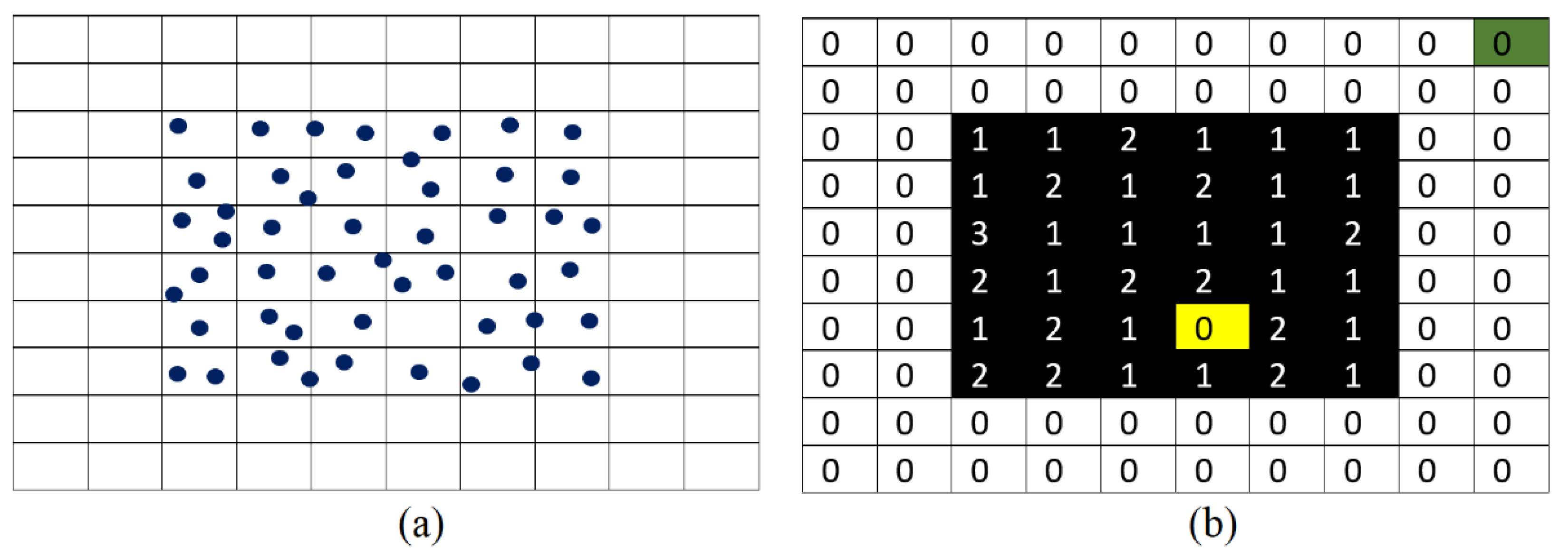
3.1. DSM Resolution Calculation

These approaches start with projecting the building point cloud onto a grid defined in the horizontal plane OXY. This grid consists of n rows and m columns and, consequently, of n × m pixels. To calculate the grid resolution (pixel size), the point density should be calculated. For this purpose, using the Theoretical Point Density (TD) provided by the scanning company, the Theoretical Mean Distance (TMD) between two neighboring points is calculated (Equation (1)) [73], where it is assumed that the distribution of points is regular and that one pixel should include at least one point; thus, the mean point density may be derived from Equation (1).
T M D = 1 T D
Assuming that the pixel size equals TMD, the building Digital Surface Model (DSM) can be calculated. From this model, the values of empty pixels inside the building body are calculated using a gradient filter. Thereafter, the number of building LiDAR points is divided by the building area to calculate the actual point density.

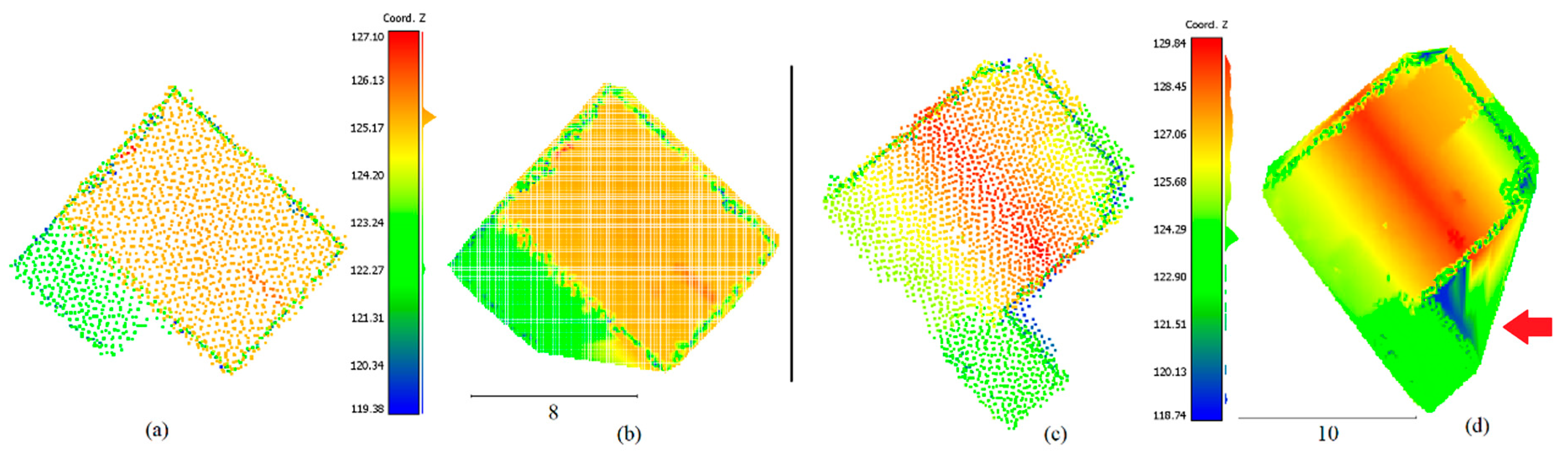
3.2. Calculation of the Building DSM

Once the resolution of the building DSM is calculated, the building point cloud is superimposed on the constructed grid, and the pixel values are assigned according to the presence of LiDAR points inside or surrounding the pixel. In this context, the pixel value is calculated depending on the Z-coordinates of points within the pixel. We take the maximum Z-coordinate values of the LiDAR points located inside the pixel. This choice has been adopted to conserve the Z-coordinate from interpolation; then, the LiDAR points will keep expressing the roof geometry.
At this stage, four kinds of empty pixels can be distinguished: first, the empty pixels located outside the building boundaries, e.g., the green cell in Figure 8b; second, empty pixels located inside the building boundaries, e.g., the yellow cell in Figure 8b; third, pixels belonging to the building body and containing only one LiDAR point; and, finally, pixels belonging to the building body and containing more than one LiDAR point (Figure 8b). Indeed, the irregular distribution of LiDAR points on the building roof regarding the LiDAR point accuracy, the roof texture, and the presence of vertical surfaces such as building facades and noisy points may produce a variant number of LiDAR points located inside each pixel.
Hence, the application of a gradient filter allows the recognition of the last type of empty pixels. If an empty pixel is located inside the building boundary, the mean Z-coordinate value of the LiDAR points located in the neighborhood of the pixel boundaries is assigned to this pixel.
Figure 9 visualizes the DSM of two buildings calculated using two different methods. In the first method, the empty pixels inside the building body are kept empty (Figure 9a,c). In contrast, in the second method, the empty pixels inside the building body are filled using a gradient filter (see the last paragraph and Figure 9b,d). It can be noted in Figure 9a,c that the empty pixels can reduce the building area, especially when the DSM resolution used is small. Also, filling the empty pixel inside the building body carries the risk of filling non-building pixels in the neighborhood of the building boundary (red arrow in Figure 9d). The last added pixel will increase the building area. Unfortunately, in the last two cases, the building area will not be correct. Finally, the colors in Figure 9 are calculated as a function of the pixel values, which were calculated using the Z-coordinate values. Indeed, the color scale is divided into three intervals represented by RGB colors, where the red color expresses the highest Z-coordinate values, and the blue color represents the lowest Z-coordinate values. However, this color scale selection allows us to understand the building geometry description.
The calculation of the building DSM permits the elimination of vertical surface points such as building facades, which may have a low point density and whose role in the building volume calculation is negligible. Also, it allows us to compensate for the missing points on the roof as well as to eliminate extra points regarding the mean point density. Moreover, the DSM matrixial form not only lightens the data volume, but it helps save the topological relationships between the neighboring points, which facilitates the modeling step. On the other hand, during the calculation of the building DSM and when filling in the missing points inside the building body, extra pixels outside the building body and adjacent to the building boundaries will be added (see red arrow in Figure 9d). Indeed, boundary pixels have similar topological values to the empty pixels inside the building’s body (see red arrow in Figure 9d). These added extra pixels outside a building’s body will increase the area of the building (Table 2). Also, the DSM resolution value (pixel size) affects the building area (Table 2). One boundary pixel will be considered to be completely covered by a building body, but the truth is that it can be partially covered by a building body. Such boundary errors will increase when the DSM resolution decreases (Table 2). In addition to the last listed factors that affect the calculated building area, classification uncertainty may also be considered. When some non-building points connected to the building body are classified as building points, these misclassified points will increase the calculated building area.
From Table 2, it can be noted that the area values, in the case of non-filling the empty pixels inside the building body, greatly increase when the DSM pixel size increases. Also, when the resolution value is smaller than the resolution calculated from the point density (0.1 m), the difference will be very large, because the voids will occupy a large area inside the building body DSM. To clarify this idea, let us compare the number of building pixels containing LiDAR points to the number of building empty pixels when different pixel sizes are considered (Table 1). It can be noted in building number 0 that when the pixel size is very small (0.1 m), the number of empty pixels equals 86% of the total number of building pixels. Whereas for the same building, when the pixel size becomes larger (0.6 m), the number of empty pixels equals 3.6% of the total number of building pixels. This huge difference in the percentage of empty pixels inside the building body DSM is mainly responsible for the great building area value difference when the empty pixels are filled or not. Also, when the DSM pixel size becomes smaller, the missing-point influence will decrease, but, unfortunately, the boundary error influence will continue to increase. Conversely, in the case of filling the empty pixels inside a building body, only the boundary-error influence will continue to be added.

3.3. Building Area Calculation and Accuracy Estimation

At this stage, one question arises: is the building DSM a better choice for calculating the building area and volume, or is the direct use of the building point cloud preferable? To calculate the building area, the direct use of the building point cloud will, of course, provide accurate results because boundary errors and empty-pixel issues will not be present. In this context, convex-hull and alpha-shape algorithms can be used to calculate the building area, starting from the LiDAR building point cloud. On the other hand, the missing building ground part due to the roof and facade presence, in addition to the low point density or/and missing facade sections in the building point cloud, means that the building point cloud will not be sufficient to directly calculate the building volume. To conclude, the direct use of the point cloud will provide an accurate result when calculating the building area starting from the LiDAR building point cloud. Conversely, to calculate the building volume starting from the LiDAR building point cloud, the direct use of the point cloud will not provide an accurate result because of the heterogeneous distribution of LiDAR points; that is why the use of the building DSM is unavoidable.
First, the point cloud is projected onto the horizontal plane OXY to calculate the building footprint area, starting from the LiDAR building point cloud. This operation allows the conversion of the 3D point cloud into a 2D point cloud. Second, the polygon boundary of the 2D building point cloud is detected using convex-hull or alpha-shape algorithms. The area of this polygon represents the building’s footprint area. This approach does not only provide an accurate result, but it also guarantees the stability of the area value.
At this stage, it is important to highlight the different concepts of building areas. Two kinds of building areas can be distinguished. The first is the building footprint area, where the underhung and overhung parts are considered simultaneously. Second is the underhung area, where the overhung parts are not considered. The calculation of the building intensity index uses the underhung area, whereas the LiDAR building point cloud allows the calculation of the building footprint area. That is why it is understandable that if the allowed overhung parts percentage is known, then the LiDAR building point cloud can provide an accurate value of the intensity index.
To estimate the accuracy of the calculated area of the target building, several kinds of errors are defined. First, errors due to the point density and errors due to the point planimetric accuracy can be estimated. On a 2D LiDAR point inside one pixel, even though it is assumed that this point is situated in the pixel center, it can exist anywhere inside this pixel boundary. The distance between the pixel center and the extreme location of the LiDAR point inside the target pixel equals d L d = 0.5 × T M D , where TMD is the mean distance between two neighboring points. The second error to be considered is the error related to the LiDAR points’ planimetric accuracy ( d L a ) . The third source of error in the building area calculation is the point cloud Classification Error (CE). If we suppose that Ar is the building footprint area, the building’s footprint geometrical form is square, and that this square side length equals L, then A r = L 2 . According to the error propagation law, the total building area error (dAr) can be described by Equation (2).
d A r = 4 × A r × d L d 2 + d L a 2 + A r × C E 2
As an example, for T M D = 0.25   m ,   d L a = 0.15   m ,   A r = 150   m 2 ,   a n d   C E = 3 % , it can be found that d L d = 0.5 × 0.25 = ± 0.125   m ; then, d A r = ± 6.57   m 2 .

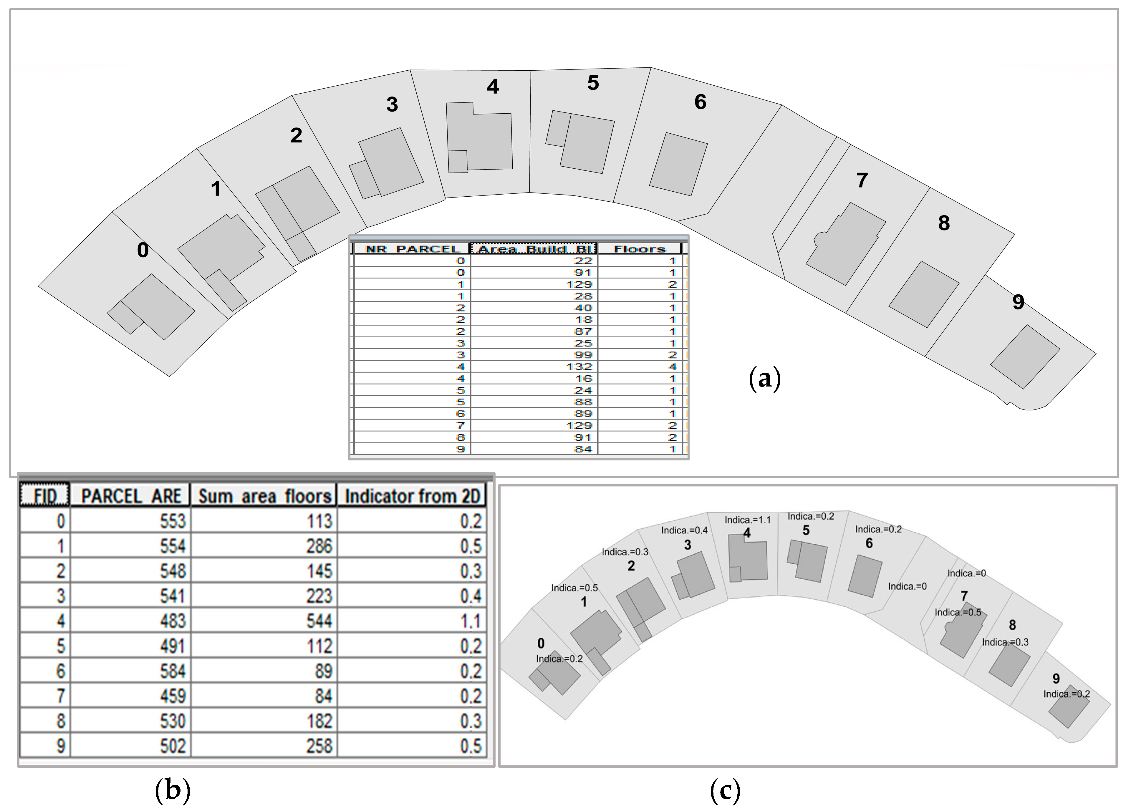
3.4. Multi-Story Building Area and Building Intensity Index

To calculate the building intensity index, the summation of all the building level areas is divided by the parcel area. For this purpose, the building’s Multi-Level Area (MLA) should be calculated. In this context, the building point cloud is segmented according to the number of levels. As the ground level has already been calculated (see Section 3), the subtraction of the ground level value from the Z-coordinate of the LiDAR points will provide the height of the LiDAR point above the ground level. This value can help to determine the number of building levels related to the LiDAR point concerned. Unfortunately, noise may generate considerable errors when the LiDAR points are processed point by point. That is why it is advisable to carry out this procedure by considering the roof facets (see Section 3.5). The average building level height can be made into an input, and then the number of levels can be calculated for each roof plane, where one building can be composed of several different masses of levels.

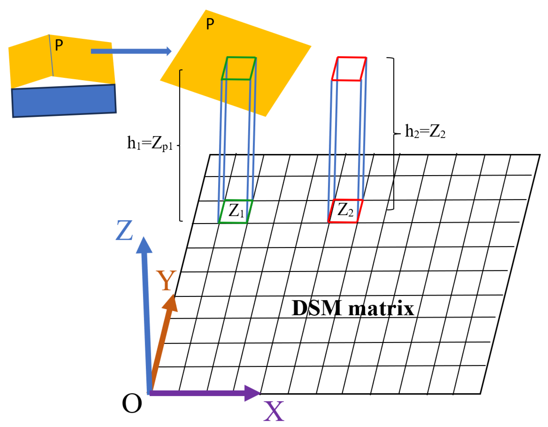
3.5. Building Volume Calculation and 3D Building Intensity Index

At this stage, the building DSM is calculated from the LiDAR point cloud in addition to the ground level, which was estimated in Section 3. These two elements are the input data for this operation. At this point, the two approaches for the building volume calculation shown in Figure 6 will be presented and discussed. The first suggested approach to calculating the building volume (see green and blue arrows in Figure 6) is based on a hypothesis that the building roof is composed of a list of planar surfaces. However, this algorithm will still be efficient despite the obtained roof deformations when no planar surfaces are present. Indeed, a non-planar surface will be detected as several neighboring patches, where each one will present a local plane. Therefore, this method can be adopted for calculating the volumes of generic buildings.
To segment the building roof according to the planar elements, the extended RANdom SAmple Consensus (RANSAC) paradigm is consecutively applied to the building DSM points within a loop to detect all roof planar facets. This algorithm selects three points randomly and fits the plane containing the selected points. Thereafter, it detects all points behaving at a minimal distance (inferior to the given threshold) to the fitted plane. This operation is iterative, where in each iteration, the number of points and the standard deviation of the newly detected plane are compared to the saved plane. If the new plane is better than the saved one regarding the two criteria used, the new plane will replace the previously saved plane. The number of iterations is calculated using a chi-square ( χ 2) distribution density function, which is a continuous probability distribution. Furthermore, the extended RANSAC algorithm loop will be stopped when the number of remaining points becomes smaller than a given threshold (3% of the building point cloud) or when the algorithm fails to detect any more planes. In each loop iteration, the detected plane will be assessed if some plane points do not belong to the main detected plane body. Hence, these points will be eliminated and reassigned to the building point cloud.
Once the roof planes are detected, the building DSM pixel values are recalculated (adjusted) according to the plane equation to which they belong. In the last step, considering the ground level, each pixel in the adjusted building DSM forms a rectangular parallelepiped, whose height equals the value of the ground level value subtracted from the pixel value, and the base area equals the square of the pixel length, which was calculated in Section 3.1. In Figure 9, the pixel of the green boundary illustrates the calculation approach. Finally, summation of all the rectangular parallelepipeds formed by the building body pixels will produce the building volume.
In this context, to obtain an accurate building volume, three additional rules will be applied as follows:
  • All building DSM pixels located outside the building boundary polygon, which was calculated in Section 3.3, will be eliminated.
  • For building boundary pixels located on the boundary polygon, only the parts situated inside that polygon will be considered.
  • Pixels belonging to the building body and having values smaller than a given threshold will be neglected. This threshold is related to the level height, i.e., the threshold will equal the ground level + l e v e l   h e i g h t 2 . Indeed, these kinds of pixels can be in connection with the building boundary, and they may represent a confusing noise. That is why they are kept at the classification stage.
One building may consist of several parts, where the number of levels for each part is different from other parts. In fact, the building roof segmentation allows for the recognition of the number of levels for different roof patches. If two neighboring patches have the same number of levels, they can be merged. This operation helps calculate a new matrix, named a different-level building map.
If we intend to calculate the building volume regardless of the number of levels, the second approach shown in Figure 7 can be applied. According to Figure 6 (blue and orange arrows), it is similar to the first approach for the building volume calculation, except that the building roof planes will not be detected, and the building DSM pixel values will not be adjusted. To calculate the building volume, the building DSM calculated in Section 3.2 will be used as the input. By considering the ground level, each pixel in the building DSM forms a rectangular parallelepiped, whose height equals the ground level value subtracted from the pixel value, and the base area equals the square of the pixel length, which was calculated in Section 3.1. In Figure 10, the pixel of the red boundary illustrates the calculation approach. Finally, summation of all the rectangular parallelepipeds formed by the building body pixels will produce the building volume.
Concerning the accuracy of the building volume calculated from the LiDAR point cloud, it is assumed that the building’s geometrical form is cubic, and that the cube side length equals L, such that the building volume V = L 3 . Similar to the building area accuracy calculation, three errors are envisaged: the error caused by the point density, the error due to the accuracy of the LiDAR points, and the error due to the LiDAR data classification accuracy.
d V = 9 × V 4 3 × d L d 2 + d L a 2 + V × C E 2
To understand Equation (3) better, let T M D = 0.25   m ,   d L a = 0.15   m ,   A r = 500   m 3 ,   a n d   C E = 3 % . Then, it can then be found that d L d = 0.5 × 0.25 = ± 0.125   m and d V = ± 36.5   m 3 .

4. Results and Discussion

In urban indicator calculations using LiDAR data, it is useful to underline the requirements for data handling and any required preprocessing steps to make such 3D data usable for urban indicator calculations. After acquiring the LiDAR point cloud of the scanned scene, it is necessary to classify the measured point cloud into two main classes: building and non-building classes; in this case, the building class represents the project focus. For this purpose, automatic classification tools based on machine learning and rule-based algorithms can be used. Additional automatic or manual enhancement tools should be used to enhance the classification results. Once a building mask is available, a region-growing algorithm is applied to detect each building point cloud individually.
Figure 11 shows the visualization of the study site point cloud using Red, Green, and Blue (RGB) colors in addition to the target building plans representing the ground truth. Ten target buildings in the study area are enumerated from zero to nine. Also, the same figure illustrates the results of the building roof point cloud segmentation. These results will be used to calculate the building volumes using the two proposed approaches presented in Figure 7.
Table 3, Table 4, Table 5 and Table 6 and Figure 12 show the obtained results for building numbers zero to six in Figure 10, and the second data sample is shown in Figure 5, where the 2D intensity index (II) is calculated by dividing the Multi-Level Area (MLA) on the parcel area. Moreover, the 3D building intensity index (3D II) is calculated by dividing the building volume on the parcel area multiplied by the mean building height. The underhung reference data (ground truth) are measured directly from architectural building plans (Figure 5). The footprint reference data (ground truth) are measured by directly digitizing the point clouds. From Table 3 and Table 5 and Figure 12, it can be noted that the obtained building footprint areas are accurate enough regarding the ground-truth reference values. Also, the great differences between the footprint and the underhung areas can be explained by the fact that the LiDAR data was measured from above, and then all the underhung parts were considered for the area calculation. At this stage, it is important to note that the area errors are considerable because the point cloud has a sparse point density (12 p/m2) and the point cloud planimetric accuracy is about ±0.15 m, in addition to the classification uncertainty of 3%. These factors also affect the volume accuracy shown in Table 4 and Table 6. Of course, to improve the accuracy of the obtained area and volume results, more accurate and dense LiDAR data should be used.
As underhung building areas cannot be measured from the LiDAR building point clouds, the building intensity indexes are estimated using the building footprint areas (Table 3), where the results are rounded to the nearest ten centimeters. It can be noted that, despite the considerable size differences between the underhung and footprint areas, some intensity index values match the ground-truth reference values, and others increase slightly (about 0.1 more than the reference value). However, if the allowed overhung parts percentage is given as the input, then the LiDAR building point cloud can provide an accurate value of the intensity index.
Regarding the building volume results in Table 4 and Table 6 and Figure 13, negligible differences can be noted between the volume values obtained by the two suggested approaches. Indeed, fitting the mean plane equation will not be able to reduce the influence of LiDAR point errors. Nevertheless, applying the extended RANSAC algorithm to segment the building roofs will be essential to calculate one building MLA. The number of building levels can be determined accurately for each roof patch, and the noisy points will be adjusted. Also, the comparison between the building Volume 2 values and the reference volume values (ground truth) (∆Vol 2 = volume 2 − Vol Ref) (Table 4) confirms the accuracy of the suggested approach. Indeed, the volume deviation values are very close to the volume accuracy values presented in the same table. Moreover, to calculate the Volume Relative Accuracy (VRA), Volume 2 of the buildings is used. The high value of the VRA may be explained by the low point density and accuracy value. To improve the volume accuracy, the LiDAR point density and accuracy should be improved, as well as the classification accuracy. Finally, the 3D building intensity index (3D II) is calculated two times using both building volume values: Volume 1 and Volume 2. It can be noted that both results are practically identical because the building volume values obtained by the two proposed approaches are very similar.
At this stage, it is important to examine the three assumptions applied in this paper (see Section 3). They concern the planar geometric form of the building ground and the building facade planar form, and how these might influence the accuracy of the indicators. Indeed, a discussion on the limitations of these assumptions in practical urban planning scenarios could provide a more balanced view. Regardless of the presence of indoor construction elements such as walls, ceilings, and floors, the building volume and height measured from indoors may not be equal to the volume measured from outdoors, especially in the case of the presence of underground parts or basements. Moreover, building facades may contain 3D elements such as decorations and terraces. The assumption of a building having vertical planar facades will not help to accurately calculate the building volume. However, the availability of extra information about buildings such as the presence of underground elements or terraces, will make LiDAR data more efficient in providing accurate building indicators.
At this stage, it is necessary to discuss the required input data accuracy for calculating the building indicators. The input data for the automatic calculation of building indicators, as mentioned in Section 1.4, are the design BIM, as-built BIM, and LiDAR data. First, the accuracy tolerance between design BIM and as-built BIM is empirically about 10 cm if high accuracy scanning is used for as-built BIM. This tolerance value is produced from four main sources: scanning accuracy, registration accuracy, georeferencing accuracy, and the anomaly of construction elements, such as walls, floors, and ceilings, from their geometrical definition used in design BIM. Also, the accuracy of airborne LiDAR data is very close to the tolerance value. In Table 3, Table 4, Table 5 and Table 6, the values of the last two columns are rounded to one decimal place, which confirms the sufficient accuracy of LiDAR data as well as as-built BIM for calculating the building indicators.
In summary, the calculated 3D indicators correlate with the classically calculated indicators and with the point-based indicators using the two methods. The buildings with classic solutions presented for the research do not take into account modern buildings created with new technologies or of various shapes and different story heights. Traditional calculations of indicators consider the sum of the areas of each story of the buildings, but they do not consider the height. This can be confusing. In contrast, the two proposed solutions for calculating the development intensity in the examined cases are consistent.

5. Conclusions

The presented research shows that in the absence of reference data, e.g., BIM data, cadastral data, and data from remote measurements, we can still calculate development intensity indicators. The simplicity of the calculations, based on remote sensing measurements, can replace cumbersome classic measurements.
Regardless of the LiDAR data acquisition cost in urban areas, which can be interpreted as being due to the high speed of measurement in addition to the high automation level of data processing, the calculated 3D building intensity indexes show a high correlation with classical indexes calculated from 2D data. This result indicates the possibility of using 3D indicators, as they more accurately reflect the built-up space. The 3D approach should be used when calculating other suggested indicators related to, e.g., the insolation of buildings and sky visibility. However, the question that still arises for discussion is this: Is it common to be able to cover a building with thousands of points from LiDAR to calculate the building indexes? Definitely, yes, and the high density of points ensures the result accuracy, which can be considered a great gain in addition to the high speed of data updating for making decisions.
Of course, if the cadastral map is available and it is faithful to the as-built city data, the cadastral map will be used for calculating the intensity indexes. Unfortunately, when the as-built city data do not match with the cadastral map, then the cadastral map needs a fast update. However, when the LiDAR data are used to calculate the intensity indicators, calculation of the building area directly from the LiDAR point cloud provides more accurate results than by using the building DSM. On the other hand, using the DSM matrixial representation of the building point cloud is essential to calculating the building volume because of the irregular distribution of LiDAR points covering the facades. However, the accuracy of the computed building area, volume, and other indicators depends on the LiDAR point cloud density and accuracy. Also, the accuracy of the building class extraction from the scanned scene plays a major role in the calculation. The adopted research activities are aimed at enabling the construction of a spatial planning portal in the future, in which it will be possible, based on the available data and tools, to visualize the planning space and to perform the necessary planning analyses. We believe that this is the future in urban planning. Airborne LiDAR data will be of vital importance in these activities.
In future research, other building indicators, such as the footprint perimeter, ratio of building height to footprint area, wall areas, envelope area, and orientation, will be investigated. Furthermore, new data from different urban typologies, in addition to other laser scanning data acquisition techniques such as UAV scanning and terrestrial mobile scanning, will also be tested with the suggested algorithm to assess its performance on various urban typologies and point cloud resolutions. Finally, future research could examine automatic updates of urban datasets using AI-based LiDAR processing.

Author Contributions

Conceptualization, F.T.K., E.L., J.S. and Z.G.; methodology, F.T.K. and E.L.; software, F.T.K.; validation, F.T.K., formal analysis, F.T.K.; resources, E.L., data curation, F.T.K. and E.L.; writing—original draft preparation, F.T.K. and E.L.; writing—review and editing, Z.G. and J.S.; visualization, F.T.K. and E.L. All authors have read and agreed to the published version of the manuscript.

Funding

This research received no external funding.

Data Availability Statement

The publication uses LAS measurement data obtained from a Polish SDI—portal run by the Central Office of Geodesy and Cartography and data from the Spatial Information Systems of Olsztyn.

Acknowledgments

We would like to thank the Central Office of Geodesy and Cartography (GUGiK) in Poland for providing LiDAR measurement data and for making data from the 3D portal available.

Conflicts of Interest

The authors declare no conflicts of interest.

References

  1. Huang, L.; Wu, J.; Yan, L. Defining and Measuring Urban Sustainability: A Review of Indicators. Landscape Ecol. 2015, 30, 1175–1193. [Google Scholar] [CrossRef]
  2. Pira, M. A Novel Taxonomy of Smart Sustainable City Indicators. Humanit. Soc. Sci. Commun. 2021, 8, 197. [Google Scholar] [CrossRef]
  3. Angelakoglou, K.; Nikolopoulos, N.; Giourka, P.; Svensson, I.-L.; Tsarchopoulos, P.; Tryferidis, A.; Tzovaras, D. A Methodological Framework for the Selection of Key Performance Indicators to Assess Smart City Solutions. Smart Cities 2019, 2, 269–306. [Google Scholar] [CrossRef]
  4. Olewiler, N. Environmental Sustainability for Urban Areas: The Role of Natural Capital Indicators. Cities 2006, 23, 184–195. [Google Scholar] [CrossRef]
  5. Nassauer, J.I.; Wu, J.G.; Xiang, W.-N. Actionable Urban Ecology in China and the World: Integrating Ecology and Planning for Sustainable Cities. Landsc. Urban Plan. 2014, 125, 207–208. [Google Scholar] [CrossRef]
  6. Jorge-Ortiz, A.; Braulio-Gonzalo, M.; Bovea, M.D. Assessing Urban Sustainability: A Proposal for Indicators, Metrics and Scoring—A Case Study in Colombia. Environ. Dev. Sustain. 2023, 25, 11789–11822. [Google Scholar] [CrossRef]
  7. Garcia, C.; López-Jiménez, P.A.; Sánchez-Romero, F.-J.; Pérez-Sánchez, M. Assessing Water Urban Systems to the Compliance of SDGs through Sustainability Indicators. Implementation in the Valencian Community. Sustain. Cities Soc. 2023, 96, 104704. [Google Scholar] [CrossRef]
  8. Gavaldà, O.; Gibbs, C.; Eicker, U. A Review of Current Evaluation Urban Sustainability Indicator Frameworks and a Proposal for Improvement. Sustainability 2023, 15, 15425. [Google Scholar] [CrossRef]
  9. Boeing, G.; Higgs, C.; Liu, S.; Giles-Corti, B.; Sallis, J.F.; Cerin, E.; Lowe, M.; Adlakha, D.; Hinckson, E.; Moudon, A.V.; et al. Using open data and open-source software to develop spatial indicators of urban design and transport features for achieving healthy and sustainable cities. Lancet Glob. Health 2022, 10, E907–E918. [Google Scholar] [CrossRef]
  10. Tan, S.; Hu, B.; Kuang, B.; Zhou, M. Regional differences and dynamic evolution of urban land green use efficiency within the Yangtze River Delta, China. Land Use Policy 2021, 106, 105449. [Google Scholar] [CrossRef]
  11. Pozoukidou, G.; Angelidou, M. Urban Planning in the 15-Minute City: Revisited under Sustainable and Smart City Developments until 2030. Smart Cities 2022, 5, 1356–1375. [Google Scholar] [CrossRef]
  12. Krüger, A.; Kolbe, T.H. Building Analysis for Urban Energy Planning Using Key Indicators on Virtual 3D City Models—The Energy Atlas Of Berlin. Int. Arch. Photogramm. Remote Sens. Spatial Inf. Sci. 2012, XXXIX-B2, 145–150. [Google Scholar] [CrossRef]
  13. Liu, B.; Guo, X.; Jiang, J. How Urban Morphology Relates to the Urban Heat Island Effect: A Multi-Indicator Study. Sustainability 2023, 15, 10787. [Google Scholar] [CrossRef]
  14. Hu, Y.; Dai, Z.; Guldmann, J.-M. Modeling the Impact of 2D/3D Urban Indicators on the Urban Heat Island over Different Seasons: A Boosted Regression Tree Approach. J. Environ. Manag. 2020, 266, 110424. [Google Scholar] [CrossRef]
  15. Biljecki, F.; Stoter, J.; Ledoux, H.; Zlatanova, S.; Çöltekin, A. Applications of 3D City Models: State of the Art Review. ISPRS Int. J. Geo-Inf. 2015, 4, 2842–2889. [Google Scholar] [CrossRef]
  16. Willenborg, B.; Sindram, M.; H. Kolbe, T. Applications of 3D City Models for a Better Understanding of the Built Environment. In Understanding of the Built Environment; Behnisch, M., Meinel, G., Eds.; Trends in Spatial Analysis and Modelling; Geotechnologies and the Environment; Springer: Cham, Switzerland, 2017; Volume 19. [Google Scholar] [CrossRef]
  17. Kang, Y. Visualization analysis of urban planning assistant decision network 3D system based on intelligent computing. Heliyon 2024, 10, e31321. [Google Scholar] [CrossRef]
  18. Brasebin, M.; Perret, J.; Mustière, S.; Weber, C. Measuring the impact of 3D data geometric modeling on spatial analysis: Illustration with Skyview factor. Usage Usability Util. 3D City Models 2012, 02001. [Google Scholar] [CrossRef]
  19. Liang, X.; Chang, J.H.; Gao, S.; Zhao, T.; Biljecki, F. Evaluating human perception of building exteriors using street view imagery. Build. Environ. 2024, 263, 111875. [Google Scholar] [CrossRef]
  20. Biljecki, F.; Lim, J.; Crawford, J.; Moraru, D.; Tauscher, H.; Konde, A.; Adouane, K.; Lawrence, S.; Janssen, P.; Stouffs, R. Extending CityGML for IFC-sourced 3D city models. Autom. Constr. 2021, 121, 103440. [Google Scholar] [CrossRef]
  21. Kutzner, T.; Chaturvedi, K.; Kolbe, T.H. CityGML 3.0: New functions open up new applications. PFG J. Photogramm. Remote Sens. Geoinf. Sci. 2020, 88, 43–61. [Google Scholar] [CrossRef]
  22. Kolbe, T.H.; Kutzner, T.; Smyth, C.S.; Nagel, C.; Roensdorf, C.; Heazel, C. OGC City Geography Markup Language (CityGML) Part 1: Conceptual Model Standard, 2021. Available online: https://www.opengis.net/doc/IS/CityGML-1/3.0 (accessed on 26 April 2025).
  23. Kutzner, T.; Smyth, C.S.; Nagel, C.; Coors, V.; Vinasco-Alvarez, D.; Ishi, N. OGC City Geography Markup Language (CityGML) Part 2: GML Encoding Standard, 2023. Available online: http://www.opengis.net/doc/IS/CityGML-2/3.0 (accessed on 26 April 2025).
  24. Biljecki, F.; Ledoux, H.; Stoter, J. An improved LOD specification for 3D building models. Computers. Environ. Urban Syst. 2016, 59, 25–37. [Google Scholar] [CrossRef]
  25. Domińczak, M. Metodyka regulacji intensywności zabudowy w ujęciu historycznym–zarys problematyki. Methodology of building density regulation—Historical aspects. Builder 2021, 294, 12–15. [Google Scholar] [CrossRef]
  26. Bansal, V.K. Use of geographic information systems in spatial planning: A case study of an institute campus. J. Comput. Civ. Eng. 2014, 28, 05014002. [Google Scholar] [CrossRef]
  27. Michalik, A.; Załuski, D.; Zwirowicz-Rutkowska, A. Rozważania nad intensywnością zabudowy w kontekście praktyki urbanistycznej oraz potencjału technologii GIS (Considerations on the intensity of development in the context of urban practice and the potential of GIS technology). Rocz. Geomatyki 2015, 13, 133–145. [Google Scholar]
  28. Michalik, A.; Zwirowicz-Rutkowska, A. Geoportal Supporting Spatial Planning in Poland: Concept and Pilot Version. Geomat. Environ. Eng. 2023, 17, 2. [Google Scholar] [CrossRef]
  29. Guler, D. Implementation of 3D spatial planning through the integration of the standards. Trans. GIS 2023, 27, 2252–2277. [Google Scholar] [CrossRef]
  30. Gui, S.; Qin, R. Automated LoD-2 model reconstruction from very-high-resolution satellite-derived digital surface model and orthophoto. ISPRS J. Photogramm. Remote Sens. 2021, 181, 1–19. [Google Scholar] [CrossRef]
  31. Lewandowicz, E.; Tarsha Kurdi, F.; Gharineiat, Z. 3D LoD2 and LoD3 Modeling of Buildings with Ornamental Towers and Turrets Based on LiDAR Data. Remote Sens. 2022, 14, 4687. [Google Scholar] [CrossRef]
  32. Tarsha Kurdi, F.; Lewandowicz, E.; Gharineiat, Z.; Shan, J. Modeling Multi-Rotunda Buildings at LoD3 Level from LiDAR Data. Remote Sens. 2023, 15, 3324. [Google Scholar] [CrossRef]
  33. Tarsha Kurdi, F.; Gharineiat, Z.; Campbell, G.; Dey, E.K.; Awrangjeb, M. Full Series Algorithm of Automatic Building Extraction and Modelling from LiDAR Data. In Proceedings of the 2021 Digital Image Computing: Techniques and Applications (DICTA), Gold Coast, Australia, 29 November–1 December 2021; pp. 1–8. [Google Scholar]
  34. Peters, R.; Dukai, B.; Vitalis, S.; Van Liempt, J.; Stoter, J. Automated 3D Reconstruction of LoD2 and LoD1 Models for All 10 Million Buildings of the Netherlands. Photogramm. Eng. Remote Sens. 2022, 88, 165–170. [Google Scholar] [CrossRef]
  35. Bizjak, M.; Žalik, B.; Štumberger, G.; Lukač, N. Large-scale estimation of buildings’ thermal load using LiDAR data. Energy Build. 2021, 231, 110626. [Google Scholar] [CrossRef]
  36. Zhang, Z.; Qian, Z.; Zhong, T.; Chen, M.; Zhang, K.; Yang, Y.; Zhu, R.; Zhang, F.; Zhang, H.; Zhou, F.; et al. Vectorized rooftop area data for 90 cities in China. Sci. Data 2022, 9, 66. [Google Scholar] [CrossRef] [PubMed]
  37. Wang, X.; Luo, Y.P.; Jiang, T.; Gong, H.; Luo, S.; Zhang, X.W. A new classification method for LIDAR data based on unbalanced support vector machine. In Proceedings of the 2011 International Symposium on Image and Data Fusion, Tengchong, China, 9–11 August 2011; pp. 1–4. [Google Scholar] [CrossRef]
  38. Wen, C.; Yang, L.; Li, X.; Peng, L.; Chi, T. Directionally constrained fully convolutional neural network for airborne LiDAR point cloud classification. ISPRS J. Photogramm. Remote Sens. 2020, 162, 50–62. [Google Scholar] [CrossRef]
  39. Maltezos, E.; Doulamis, A.; Doulamis, N.; Ioannidis, C. Building extraction from LiDAR data applying deep convolutional neural networks. IEEE Geosci. Remote Sens. Lett. 2018, 16, 155–159. [Google Scholar] [CrossRef]
  40. Yuan, J. Learning building extraction in aerial scenes with convolutional networks. IEEE Trans. Pattern Anal. Mach. Intell. 2017, 40, 2793–2798. [Google Scholar] [CrossRef]
  41. Kuras, A.; Brell, M.; Rizzi, J.; Burud, I. Hyperspectral and Lidar Data Applied to the Urban Land Cover Machine Learning and Neural-Network-Based Classification: A Review. Remote Sens. 2021, 13, 3393. [Google Scholar] [CrossRef]
  42. Zhou, L.; Geng, J.; Jiang, W. Joint Classification of Hyperspectral and LiDAR Data Based on Position-Channel Cooperative Attention Network. Remote Sens. 2022, 14, 3247. [Google Scholar] [CrossRef]
  43. Pang, H.E.; Biljecki, F. 3D building reconstruction from single street view images using deep learning. Int. J. Appl. Earth Obs. Geoinf. 2022, 112, 102859. [Google Scholar] [CrossRef]
  44. Xu, Y.; Stilla, U. Towards Building and Civil Infrastructure Reconstruction from Point Clouds: A Review on Data and KeyTechniques. IEEE J. Sel. Top. Appl. Earth Obs. Remote Sens. 2021, 14, 2857–2885. [Google Scholar] [CrossRef]
  45. Zhuang, J.; Li, G.; Xu, H.; Xu, J.; Tian, R. TEXT-TO-CITY Controllable 3D Urban Block Generation with Latent Diffusion Model. In Proceedings of the 29th International Conference of the Association for Computer-Aided Architectural Design Research in Asia (CAADRIA), Singapore, 20–26 April 2024; Volume 2, pp. 169–178. Available online: https://www.researchgate.net/publication/380124047_TEXT-TO-ITYControlla-ble_3D_Urban_Block_Generation_with_Latent_Diffusion_Model (accessed on 14 August 2024).
  46. Li, J.; Yang, B.; Chen, C.; Habib, A. NRLI-UAV: Non-rigid registration of sequential raw laser scans and images for low-cost UAV LiDAR point cloud quality improvement. ISPRS J. Photogramm. Remote Sens. 2019, 158, 123–145. [Google Scholar] [CrossRef]
  47. Mongus, D.; Lukač, N.; Žalik, B. Ground and building extraction from LiDAR data based on differential mor-phological profiles and locally fitted surfaces. ISPRS J. Photogramm. Remote Sens. 2014, 93, 145–156. [Google Scholar] [CrossRef]
  48. Yang, B.; Li, J. A hierarchical approach for refining point cloud quality of a low cost UAV LiDAR system in the urban environment. ISPRS J. Photogramm. Remote Sens. 2022, 183, 403–421. [Google Scholar] [CrossRef]
  49. Gilani, S.A.N.; Awrangjeb, M.; Lu, G. An Automatic Building Extraction and Regularisation Technique Using LiDAR Point Cloud Data and Orthoimage. Remote Sens. 2016, 8, 258. [Google Scholar] [CrossRef]
  50. Lukač, N.; Mongus, D.; Žalik, B.; Štumberger, G.; Bizjak, M. Novel GPU-accelerated high-resolution solar potential estimation in urban areas by using a modified diffuse irradiance model. Appl. Energy 2024, 353 Pt A, 122129. [Google Scholar] [CrossRef]
  51. Orthuber, E.; Avbelj, J. 3D Building Reconstruction from Lidar Point Clouds by Adaptive Dual Contouring. ISPRS Ann. Photogramm. Remote Sens. Spatial Inf. Sci. 2015, II-3/W4, 157–164. [Google Scholar] [CrossRef]
  52. Bizjak, M.; Mongus, D.; Žalik, B.; Lukač, N. Novel Half-Spaces Based 3D Building Reconstruction Using Airborne LiDAR Data. Remote Sens. 2023, 15, 1269. [Google Scholar] [CrossRef]
  53. Tarsha Kurdi, F.; Lewandowicz, E.; Shan, J.; Gharineiat, Z. 3D modeling and visualization of single tree Lidar point cloud using matrixial form. IEEE J. Sel. Top. Appl. Earth Obs. Remote Sens. 2024, 17, 2024. [Google Scholar] [CrossRef]
  54. Tarsha Kurdi, F.; Amakhchan, W.; Gharineiat, Z. Random Forest machine learning technique for automatic vegetation detection and modeling in LiDAR data. Int. J. Environ. Sci. Nat. Resour. 2021, 28, 556234. [Google Scholar]
  55. Tarsha Kurdi, F.; Lewandowicz, E.; Gharineiat, Z.; Shan, J. Accurate Calculation of Upper Biomass Volume of Single Trees Using Matrixial Representation of LiDAR Data. Remote Sens. 2024, 16, 2220. [Google Scholar] [CrossRef]
  56. Dong, L.; Du, H.; Han, N.; Li, X.; Zhu, D.; Mao, F.; Zhang, M.; Zheng, J.; Liu, H.; Huang, Z.; et al. Application of Convolutional Neural Network on Lei Bamboo Above-Ground-Biomass (AGB) Estimation Using Worldview-2. Remote Sens. 2020, 12, 958. [Google Scholar] [CrossRef]
  57. Zhou, L.; Xuejian, L.; Bo, Z.; Jie, X.; Yulin, G.; Cheng, T.; Huaguo, H.; Huaqiang, D. Estimating 3D Green Volume and Aboveground Biomass of Urban Forest Trees by UAV-Lidar. Remote Sens. 2022, 14, 5211. [Google Scholar] [CrossRef]
  58. Lucchi, E.; Buda, A. Urban green rating systems: Insights for balancing sustainable principles and heritage conservation for neighbourhood and cities renovation planning. Renew. Sustain. Energy Rev. 2022, 161, 112324. [Google Scholar] [CrossRef]
  59. Richa, J.P.; Deschaud, J.-E.; Goulette, F.; Dalmasso, N. AdaSplats: Adaptive Splatting of Point Clouds for Accurate 3D Modeling and Real-Time High-Fidelity LiDAR Simulation. Remote Sens. 2022, 14, 6262. [Google Scholar] [CrossRef]
  60. Biljecki, F.; Shin Chow, Y. Global Building Morphology Indicators. Comput. Environ. Urban Syst. 2022, 95, 101809. [Google Scholar] [CrossRef]
  61. Bibri, S.E. A novel model for data-driven smart sustainable cities of the future: The institutional transformations required for balancing and advancing the three goals of sustainability. Energy Inform. 2021, 4, 1. [Google Scholar] [CrossRef]
  62. USTAWA z dnia 27 marca 2003 r. o Planowaniu i Zagospodarowaniu Przestrzennym. Tekst jednolity z 2023 r. t.j. Dz. U. z 2023 Nr. 80 poz. 717, s. 20-21. (ACT of 27 March 2003 on Spatial Planning and Development. Consolidated Text of 2023, i.e., Journal of Laws of 2023, No. 80 Items 717, s 20-21). Available online: https://isap.sejm.gov.pl/isap.nsf/download.xsp/WDU20030800717/U/D20030717Lj.pdf (accessed on 26 April 2025).
  63. Rozporządzenie Ministra Rozwoju I Technologii z dnia 15 lipca 2024 r. w Sprawie Sposobu Ustalania Wymagań Dotyczących Nowej Zabudowy i Zagospodarowania Terenu w Przypadku Braku Miejscowego Planu Zagospodarowania Przestrzennego. Dziennik Ustaw 2024 poz. 1116, s. 1-2. (Regulation of the Minister of Development and Technology of 15 July 2024 on the Method of Determining the Requirements for New Development and Land Development in the Absence of a Local Spatial Development Plan). Journal of Laws of 2024, Items 1116, s. 1-2. Available online: https://isap.sejm.gov.pl/isap.nsf/download.xsp/WDU20240001116/O/D20241116.pdf (accessed on 26 April 2025).
  64. Chen, J.; Chuanbin, Z.; Feng, L. Quantifying the green view indicator for assessing urban greening quality: An analysis based on Internet-crawling street view data. Ecol. Indic. 2020, 113, 106192. [Google Scholar] [CrossRef]
  65. Sargent, I.; Holland, D.; Harding, J. The Building Blocks of User-Focused 3D City Models. ISPRS Int. J. Geo-Inf. 2015, 4, 2890–2904. [Google Scholar] [CrossRef]
  66. Jjumba, A.; Dragićević, S. Sppatial indices for measuring three-dimensional patterns in a voxel-based space. J. Geogr. Syst. 2016, 18, 183–204. [Google Scholar] [CrossRef]
  67. McTegg, S.J.; Tarsha Kurdi, F.; Simmons, S.; Gharineiat, Z. Comparative approach of unmanned aerial vehicle restrictions in controlled airspaces. Remote Sens. 2022, 14, 822. [Google Scholar] [CrossRef]
  68. Bydłosz, J.; Bieda, A.; Parzych, P. The Implementation of Spatial Planning Objects in a 3D Cadastral Model. ISPRS Int. J. Geo-Inf. 2018, 7, 153. [Google Scholar] [CrossRef]
  69. Indrajit, A.; van Loenen, B.; Ploeger, H.; van Oosterom, P. Developing a spatial planning information package in ISO 19152 land administration domain model. Land Use Policy 2020, 98, 104111. [Google Scholar] [CrossRef]
  70. Wolak, P. Topographic Data as a Basis for 3D Visualization Using Object Models Available in the GIS Program and Other Libraries. Engineering Diploma Thesis, University of Warmia and Mazury in Olsztyn, Olsztyn, Poland, 2025. [Google Scholar]
  71. Schutz, M.; Porte, L. FreeBSD (2-Clause BSD). Available online: https://github.com/potree/potree (accessed on 26 April 2025).
  72. Tarsha Kurdi, F.; Awrangjeb, M.; Munir, N. Automatic filtering and 2D modelling of LiDAR building point cloud. Trans. GIS J. 2021, 25, 164–188. [Google Scholar] [CrossRef]
  73. Tarsha Kurdi, F.; Landes, T.; Grussenmeyer, P.; Smigiel, E. New approach for automatic detection of buildings in airborne laser scanner data using first echo only. In Proceedings of the ISPRS Commission III Symposium, Photogrammetric Computer Vision, Bonn, Germany, 20–22 September 2006; International Archives of Photogrammetry and Remote Sensing and Spatial Information Sciences; International Society of Photogrammetry and Remote Sensing (ISPRS): Hannover, Germany, 2006; Volume XXXVI, Part 3, pp. 25–30. [Google Scholar]
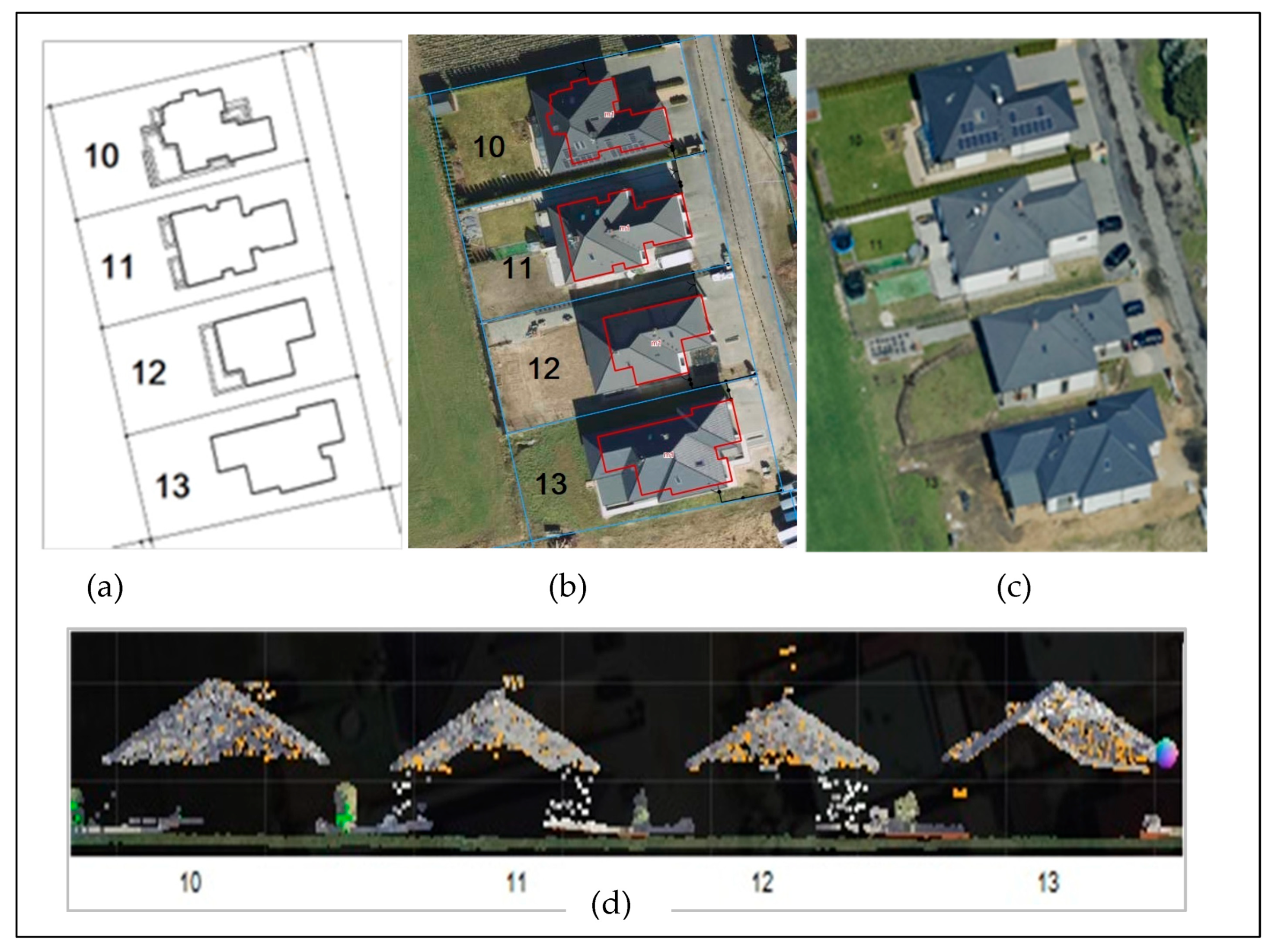
Figure 1. Visual example of the refined LODs for a residential building. Reprinted with permission from Ref. [24]. 2025, Elsevier.
Electronics 14 01821 g001
Figure 2. Illustration of independent indicators at the building level [60].
Electronics 14 01821 g002
Figure 3. Building models generated based on (a) point cloud LiDAR; (b) cadastral data and with modification H from LiDAR data; and (c) cadastral data and the number of stories with an assumed story height of 3 m [70].
Electronics 14 01821 g003
Figure 4. Selected buildings for this research study: (a) Orthophoto map, (b) Cadastral data (ground truth); (c,d) LiDAR data.
Electronics 14 01821 g004
Figure 5. Selected buildings in the second dataset: (a) Cadastral data with building and objects related to the building (terraces, stairs) (ground truth); (b) Cadastral data of buildings with orthophoto image; (c) Orthophoto map; (d) LiDAR data.
Electronics 14 01821 g005
Figure 6. Cadastral data (ground truth). Buildings are presented as blocks of buildings with different functions, often with varying numbers of stories. (a) Graphical and attribute data; (b) Data for the calculation of plot building intensity indicators, where the indicator from the 2D data is the 2D building intensity index; (c) Visualization of the calculated indicators.
Electronics 14 01821 g006
Figure 7. Two workflows for the building volume calculation using the LiDAR point cloud; the blue arrows belong to both approaches; the orange arrows and green arrows are for the first and second approaches, respectively.
Electronics 14 01821 g007
Figure 8. Building DSM calculation: (a) Superimposition of the LiDAR point cloud on the 2D grid; blue circles represent LiDAR points; (b) Black pixels represent the building body, and the numbers represent the number of LiDAR points inside the pixel; the yellow pixel is an example of an empty pixel inside the building body, while the green pixel is an empty pixel outside the building body.
Electronics 14 01821 g008
Figure 9. Building DSM: (a,b) are for Building 0; (c,d) are for Building 1; (a,c) without filling empty pixels inside the building body; (b,d) with filling empty pixels inside the building body. Red arrow points to extra pixels adjacent to the building boundaries from the outside.
Electronics 14 01821 g009
Figure 10. Calculation of the roof height for two building DSM pixels using two proposed approaches. Z1 and Z2 are DSM pixel values for the green and red pixels; h1 is the roof height calculated from the roof plane equation; h2 is the roof height considered directly from the DSM; and P is a roof plane.
Electronics 14 01821 g010
Figure 11. Results of building roof segmentation. (a) Orthophoto visualization with enumerated buildings and enumerated building plans (ground truth); (bk) Visualization of the roof segmentation results for building numbers zero to nine (as in Figure 6).
Electronics 14 01821 g011
Figure 12. Comparison of building footprint areas with ground-truth values.
Electronics 14 01821 g012
Figure 13. Comparison of building volume with ground-truth values.
Electronics 14 01821 g013
Table 1. Cadastral data from the second dataset (ground truth).
Parcel Area m2Building Area m2FloorIndicator
1083617510.2
1181721510.3
1281616810.2
1381823210.3
Table 2. Areas of Buildings 0, 1, 5, and 6 at different DSM resolutions for two cases with and without filling empty pixels inside the building body.
Building
ID
Number
of Points
DSM
Pixel Size (m)
Number of Building Pixels Containing LiDAR PointsNumber of Empty Building PixelsArea Without Filling
Empty Pixels (m2)
Area with Filling
Empty Pixels (m2)
Reference
Area (Ground Truth) (m2)
020940.1019771210219.77140.79113
0.25147081591.88142.81
0.4086149137.76145.6
0.6040015144149.4
132720.10305520,25230.55233.07157
0.2523201431145234.44
0.401334150213.38237.44
0.6062057223.2243.72
526740.1025731617125.73187.44112
0.2520351014127.19190.56
0.40116736186.72192.48
0.605437.44195.48198.00
616640.10160010,84616.00124.4689
0.25125775678.56125.81
0.4073858118.08127.36
0.6035015126.00131.40
Table 3. Calculation of building areas and the 2D intensity index; the building numbering is taken from Figure 3 and Figure 10. Ref: Reference (ground truth); MLA: Multi-Level Area; II: building intensity index.
Building IDFootprint Area (m2)Footprint Ref Area (Ground Truth) (m2)Underhung Ref Area (Ground Truth) (m2)Footprint MLA (m2)Underhung MLA Ref (Ground Truth) (m2)Area Error (m2)Parcel Area (Ground Truth) (m2)II %II Ref (Ground Truth) %
0131.35129.99113131.3511314.285530.20.2
1205.26200.53157339.5228620.315540.60.5
2218.71221.97145218.7114520.525480.40.3
3163.08162.62124263.0922312.865410.50.4
4196.78193.67148602.3154423.324831.21.1
5175.1171.51112175.111219.914910.40.2
6112.6108.5289112.60898.615840.20.2
Table 4. Calculation of building volumes and the 3D building intensity index. Building numbering is taken from Figure 4; Vol1 is calculated according to the first suggested approach, while Vol 2 is calculated according to the second suggested approach (see Figure 6); VRA is the Volume Relative Accuracy; 3D II is the 3D building intensity index.
Building
ID
Vol 1 (m3)Vol 2 (m3)Vol Ref (m3) (Ground Truth)∆Vol 2Vol
Error (m3)
VRA (%)3D II 13D II 2
0860.56860.32818.2942.0358.956.90.30.3
11454.251454.351378.3775.9886.936.00.50.5
21371.751371.251283.6787.5883.216.10.50.5
3914.82914.671015.79−101.1261.656.70.30.3
41621.711623.821522.85100.9794.365.80.70.7
51423.811429.361316.87112.4985.566.00.60.6
6619.46618.01618.29−0.2846.457.50.20.2
Table 5. Calculation of building areas and the 2D intensity index for the second dataset sample.
Building
ID
Vol 1 (m3)Vol 2 (m3)Vol
Error (m3)
VRA (%)3D II 13D II 2
101332.181312.6386.426.50.30.3
11862.55869.4467.357.80.20.2
12905.57896.2470.427.80.20.2
131450.341441.8092.526.40.40.4
Table 6. Calculation of building volumes and the 3D building intensity index for the second dataset sample (Figure 4); Vol 1 is calculated according to the first suggested approach, while Vol 2 is calculated according to the second suggested approach (see Figure 6); VRA is the Volume Relative Accuracy; 3D II is the 3D building intensity index.
Building IDFootprint Area (m2)Footprint Ref Area (Ground Truth) (m2)Underhung Ref Area (Ground Truth) (m2)Footprint MLA (m2)Underhung MLA Ref (Ground Truth) (m2)Area Error (m2)Parcel Area (Ground Truth) (m2)II %II Ref (Ground Truth) %
10250.65248.34175.00250.65175.0030.268360.30.2
11244.42245.86215.00244.42215.0022.838170.30.3
12229.56230.05168.50229.56168.5023.658160.30.2
13306.19305.47233.5306.19233.532.638180.40.3
Disclaimer/Publisher’s Note: The statements, opinions and data contained in all publications are solely those of the individual author(s) and contributor(s) and not of MDPI and/or the editor(s). MDPI and/or the editor(s) disclaim responsibility for any injury to people or property resulting from any ideas, methods, instructions or products referred to in the content.

