Abstract
The advancement of autonomous vehicles has shifted from modular pipeline architectures to end-to-end frameworks, enabling direct learning of control policies from sensory inputs. While frame-based RGB cameras are commonly utilized, they face challenges in dynamic environments, such as motion blur and varying illumination. Alternatively, event-based cameras, with their high temporal resolution and wide dynamic range, offer a promising solution. However, existing end-to-end models for event camera inputs are primarily constructed using traditional convolutional networks and time-sequence models (e.g., Recurrent Neural Networks, RNNs), which suffer from large parameter counts and excessive redundant computations. To address this gap, we propose LiS-Net, a novel framework that incorporates brain-inspired neural networks to construct the overall architecture, applying it to the task of end-to-end steering prediction. The core of LiS-Net is a liquid neural network, which is designed to simulate the behavior of C. elegans neurons for modeling purposes. By leveraging the strengths of event cameras and brain-inspired computation, LiS-Net achieves superior accuracy, smoothness, and efficiency. Specifically, LiS-Net outperforms existing models with the lowest RMSE and MAE, indicating better accuracy, while also maintaining the fewest number of neurons and achieving competitive FLOPs results, showcasing its computational efficiency. Experiments on the simulated EventScape dataset demonstrate its robustness, while validation on our self-collected dataset showcases its generalization capability. We also release the collected dataset comprising synchronized event cameras, RGB cameras, and GPS and CAN data. LiS-Net lays the foundation for scalable and efficient autonomous driving solutions by integrating bio-inspired sensors with brain-inspired computation.
1. Introduction
The development of autonomous vehicles has gradually evolved from modular pipelines to end-to-end approaches, primarily to address the high costs associated with handling corner cases in rule-based modular methods. In modular pipelines [1], standalone components for localization, perception, planning, and control work collaboratively to generate feasible actions for autonomous vehicles. This approach emphasizes the integration of various modules to ensure reliability and performance. However, end-to-end approaches [2], which aim to directly learn a mapping function between sensory inputs and vehicle actuators using neural networks, eliminate the need for explicit modular segmentation. This paradigm, often categorized under imitation learning, relies on collecting expert datasets and training neural networks to mimic expert behavior for longitudinal or lateral control.
Within end-to-end frameworks, frame-based RGB cameras have been a predominant input modality, demonstrating impressive results in learning the mapping from visual inputs to actions. These systems excel in structured environments but face challenges in capturing reliable and comprehensive scene information in unstructured or dynamic scenarios. The primary limitation of frame-based cameras lies in their inability to capture fast-moving objects or sudden scene changes with high fidelity. Since they rely on capturing frames at fixed intervals, there is a delay between frames that can lead to motion blur, particularly in high-speed environments. This results in a loss of temporal information and can hinder the vehicle’s ability to respond to quick or unpredictable changes in the environment, such as a pedestrian suddenly crossing the road or a rapidly changing traffic light.
In recent years, event-based sensors have emerged as a promising alternative for autonomous driving. Unlike traditional frame-based cameras, event cameras capture per-pixel brightness changes as asynchronous events, offering higher temporal resolution, wider dynamic range, and reduced susceptibility to motion blur. This mechanism is more analogous to the human eye’s triggering process, which responds to dynamic changes in the scene rather than capturing static frames at fixed intervals. These characteristics make event cameras well-suited for dynamic and challenging driving environments, providing low-latency and low-bandwidth advantages. Specifically, event cameras achieve sub-microsecond latency, with pixel-level events being transmitted as soon as changes are detected. On the lab bench, latency is around 10 μs, and in real-world conditions, it can be as low as sub-millisecond [3]. This rapid response enables event cameras to capture fast-moving objects with minimal delay, making them ideal for real-time applications in autonomous driving.
As for static information, event-based cameras can still capture it by integrating mechanisms that track background changes over time. While event cameras focus on detecting dynamic events, they can also record static elements through continuous monitoring of the scene. Some designs, such as the Asynchronous Time-Based Image Sensor (ATIS) [4], and Dynamic and Active Pixel Vision Sensor (DAVIS) [5], incorporate additional subpixels to measure absolute intensity, allowing the camera to capture static brightness information alongside dynamic events. This enables event-based cameras to provide a more comprehensive view of the environment, processing both dynamic and static elements efficiently.
Humans achieve robust movements and accomplish tasks by perceiving geometric features and dynamic information in their environment through visual observation and interactive evaluation. Emulating this human perception-control mechanism provides a viable framework for designing end-to-end algorithms. However, most current end-to-end models output control actions with event camera input are constructed using standard convolutional neural networks (CNNs), such as ResNet [6]. Lacking a neural basis, these networks struggle to effectively capture the complex perception-control processes required for autonomous driving, making it difficult to achieve high levels of generalizability and robustness. Moreover, these networks often contain a large number of parameters, leading to redundant computations and repeated processing of unnecessary events, which reduces their efficiency and practicality.
Inspired by Neural Circuit Policies (NCPs) [7], designing network models from a brain-inspired perspective could be a promising direction. NCPs draw inspiration from the neural computations observed in biological brains, incorporating increased computational capabilities per neuron to create sparse, interpretable networks. These models have demonstrated exceptional performance in tasks like lane-keeping, where small networks with only a few neurons have outperformed state-of-the-art methods in directly learning to steer a vehicle from high-dimensional visual RGB inputs.
We believe that brain-inspired networks are a choice for constructing end-to-end models with event camera input. On the one hand, event cameras, designed to mimic the way biological eyes perceive changes in brightness, naturally align with the computational principles of brain-inspired networks like NCPs. On the other hand, brain-inspired networks have been shown to capture more effective causal relationships with fewer neurons, which aligns well with the current needs for processing event camera data. To address this gap, our work investigates the capability of brain-inspired networks to learn end-to-end steering predictions using event-based inputs in autonomous driving scenarios.
To achieve this goal, we propose LiS-Net, a novel framework that combines the strengths of event cameras and brain-inspired neural networks. By leveraging the unique properties of event-based data, LiS-Net can learn robust, efficient, and interpretable control policies for end-to-end steering prediction. By combining bio-inspired sensors with brain-inspired computation, LiS-Net demonstrates the potential to pave the way for robust, scalable, and efficient autonomous driving solutions.
The architecture of LiS-Net introduces a novel integration of event camera data with brain-inspired neural networks to predict steering angles in an end-to-end manner. This framework incorporates four key components: tensorization, a convolutional feature extractor, a brain-inspired liquid neural network, and a smooth adjustment module. The process begins with the preprocessing of raw event data, which are converted into a structured tensor format, suitable for downstream processing. The preprocessed tensors are then passed into a convolutional feature extractor that learns spatial representations from the input data. These features are subsequently fed into the brain-inspired liquid neural network, which is designed to capture the temporal dependencies and dynamic patterns inherent in event-based data. The final step involves a smooth adjustment module that refines the predictions, ensuring both accuracy and temporal smoothness in the steering angle output. To thoroughly assess the robustness and generalizability of LiS-Net, we conducted experiments using the Carla simulation dataset EventScape for training and testing, and we further validated the trained model on a self-collected dataset that includes multiple sensors, such as event cameras, frame-based RGB cameras, GPS, and Controller Area Network (CAN) data. The deployment of the model on real-world data not only extends its validation beyond simulated environments but also provides a comprehensive evaluation of its performance in diverse conditions.
The main contributions of this work are as follows:
- Integration of brain-inspired sensor inputs with brain-inspired neural networks: We first introduce event camera inputs combined with brain-inspired Neural Circuit Policies (NCP) for end-to-end steering prediction, setting a new baseline and highlighting the potential of bio-inspired sensors and computation.
- Continuous Dynamic Modeling and Performance Analysis of LiS-Net: Inspired by the continuous state transitions of biological neurons, LiS-Net preprocesses event-based data and uses a differentiable approach to model neurons with continuous dynamics. This enables more accurate temporal information capture and better environmental modeling. By continuously modeling neuron transitions, LiS-Net ensures temporal accuracy and smoothness in end-to-end steering prediction. Trained and tested on simulated datasets, LiS-Net outperforms traditional networks in RMSE and MAE. Validation on real-world data shows LiS-Net’s efficiency with fewer neurons and relatively fewer FLOPs, demonstrating generalization for autonomous driving.
- Dataset contribution: This work also contributes to the research community by providing a self-collected dataset that includes synchronized recordings from multiple sensors, including an RGB camera, event camera, and Controller Area Network (CAN) data. This dataset enables the evaluation of model generalization to different real-world driving environments and provides valuable resources for future research.
The dataset and codes are released at https://github.com/CocoYi-Claire/LiS-Net, accessed on 25 April 2025.
2. Related Work and Key Elements
2.1. End-to-End Control Learning for Autonomous Driving
2.1.1. Architectural Paradigms: Modular vs. End-to-End
The modular architecture decomposes the autonomous driving pipeline into a series of discrete subtasks, as illustrated in the upper part of Figure 1. It links sensory inputs to control outputs through a structured sequence of components. The primary modules typically include perception, localization, mapping, planning, and control [8]. Raw sensor data are first processed by the perception module to detect obstacles [9], while the localization module estimates the vehicle’s position [10]. Based on this information, the planning and prediction modules compute an optimal and safe driving trajectory [11]. Finally, the motion control module generates low-level control commands to follow the planned trajectory and ensure safe navigation.
In contrast, the end-to-end architecture directly maps raw sensory data to driving commands, bypassing traditional sub-modules such as perception and planning, thereby simplifying the driving pipeline (as shown in the lower part of Figure 1). This approach enables continuous learning from data, allowing the system to perceive its environment and make decisions in a manner similar to human drivers. A pioneering example of this approach is Pomerleau’s Alvinn system [12], which trained a three-layer neural network to predict steering angles directly from sensory input. Modern end-to-end models can take a wide range of sensor inputs, including camera images [13,14,15], LiDAR scans [16,17,18], navigation instructions [14,19], and vehicle dynamics data such as speed. These inputs are processed by a backbone network that outputs driving commands, such as acceleration, steering, and braking, along with optional auxiliary outputs such as cost maps, interpretable features, and other supportive signals for enhanced safety and transparency.
In summary, modular architectures offer high interpretability and ease of debugging, as each module operates independently. This structure allows for systematic analysis, fault isolation, and modular upgrades or replacements, which improve the scalability and flexibility of the system. On the other hand, end-to-end architectures reduce the complexity of inter-module communication, enabling faster response times and higher computational efficiency. Since the entire system is trained holistically, it benefits from data-driven optimization and can continuously adapt to complex and dynamic environments. Considering these trade-offs, this study adopts an end-to-end approach for the design of the proposed driving network.
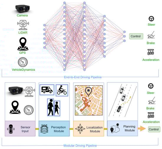
Figure 1.
Comparison between end-to-end and modular pipelines [20]. Reprinted with permission from Ref. [20]. Copyright © 2025, IEEE.
2.1.2. Network Policy for End-to-End Control Learning
End-to-end learning for lateral control in autonomous driving, which directly predicts steering angles from visual observations, offers a contrast to the traditional modular approach that includes perception, localization, and motion planning. There are two primary approaches to implementing end-to-end driving: imitation learning (IL) [16,17] and reinforcement learning (RL) [21]. IL is typically formulated as a supervised learning problem, where a model is trained to imitate expert human driving behavior based on demonstration data. However, IL suffers from limited generalizability, as training data often fail to cover the full diversity of real-world scenarios. In contrast, RL enables an agent to learn driving behavior through interaction with the environment, with the objective of maximizing cumulative rewards [22]. Although RL allows for online adaptation and exploration, it is generally less data-efficient compared to IL.
ALVINN [12], introduced in 1998, was the first visuomotor network to learn steering based on images using a simple 3-layer neural network. Following this, NVIDIA developed a convolutional neural network (CNN) that predicted steering angles for highway driving by processing images from a front-facing camera [23]. This was extended by Karsli, who proposed a CNN architecture for steering angle prediction from camera images [24]. Other studies, like [25], integrated CNNs with LSTMs to model vehicle motion and predict steering based on camera data and vehicle states. Kim and Canny [26] utilized attention heat maps to interpret frame-based RGB data for steering prediction. Additionally, Azam [27] applied behavioral cloning to train a neural network that predicts steering, throttle, brake, and torque commands from visual data, further refining control predictions using deep neural networks.
While these approaches demonstrate the feasibility of learning steering policies directly from visual inputs, several limitations persist. First, frame-based RGB cameras struggle with motion blur and extreme lighting variations, necessitating heavy data augmentation. Second, the reliance on supervised learning requires costly human demonstration datasets, potentially inheriting biases from expert drivers. Recent attempts to address these issues include self-supervised depth estimation and hybrid sensor fusion, though real-time deployment remains challenging due to computational constraints.
2.1.3. End-to-End Learning: From Monocular to Multimodal Perception
Autonomous driving requires robust mapping of perception to control in dynamic environments. Early end-to-end approaches predominantly relied on monocular RGB cameras due to their simplicity and low cost, but recent advances explore multimodal sensing to overcome inherent limitations. For example, binocular systems [28,29] can leverage stereo disparity for 3D perception, achieving 30FPS obstacle detection at 15W. These studies collectively demonstrate binocular vision’s dual competence in dynamic obstacle localization and infrastructure sensing, advancing smart mobility through hardware–algorithm co-design.
Focusing on multimodality, Sobh et al. [30] employed CARLA to design a continual imitation learning (CIL) approach that integrates camera and LiDAR data using a mid-level fusion strategy. Specifically, semantic segmentation derived from RGB images is fused with two LiDAR-based representations: a bird’s-eye view and a polar grid. Similarly, Khan et al. [31] proposed an end-to-end CNN model using CARLA, which first learns steering prediction from depth (Z-buffer) alone, then refines this with mid-level fusion of depth features and semantic segmentation extracted from RGB images. This two-stage design allows semantic segmentation to be conditioned on depth via backpropagation, highlighting the role of structured fusion in multimodal learning.
While monocular vision remains attractive due to its low cost and system simplicity, it suffers from inherent depth ambiguity and limited robustness in complex environments. In contrast, multimodal perception—though more computationally demanding—offers richer, complementary information that enhances driving policy learning and generalization, especially under challenging conditions. Balancing efficiency and performance remains a key challenge in advancing end-to-end autonomous driving systems.
2.2. Event Cameras for Autonomous Driving
2.2.1. Sensor Characteristics and Advantages
Event cameras, also known as Dynamic Vision Sensors (DVSs) [32,33,34], have revolutionized the way visual data are captured, moving away from traditional frame-based systems. Unlike conventional cameras that capture static images at fixed intervals, event cameras detect and record changes in the scene, producing a continuous stream of events. Each event corresponds to a significant change in light intensity at a specific pixel, including its timestamp and polarity. This asynchronous operation enables event cameras to achieve high temporal resolution, low latency, and reduced power consumption by processing only dynamic information, eliminating redundancy. Furthermore, event cameras offer a high dynamic range, making them effective in a variety of lighting conditions, including very bright or low-light environments. The technology has been widely explored for its advantages in real-time applications, such as high-speed motion tracking [35,36] and robotics [37,38], where fast decision-making and efficient data handling are crucial. Research has also highlighted its potential in low-power and high-throughput scenarios, making it suitable for battery-powered devices and long-term monitoring applications [39]. Despite its benefits, challenges remain in data processing and integration with traditional systems, but ongoing advancements continue to expand the utility and applicability of event cameras.
2.2.2. End-to-End Learning with Event Data
Early efforts in end-to-end learning for lateral control of autonomous vehicles primarily relied on visual data from frame-based cameras. While effective to some extent, these cameras are prone to challenges such as illumination variation, motion blur, and sun glare. To overcome these limitations, researchers have proposed integrating event cameras, which operate asynchronously and capture pixel-level brightness changes. Unlike frame-based cameras, event cameras produce sparse, high-temporal-resolution signals with low latency and a wide dynamic range, making them well-suited for handling dynamic scenes [3].
The complementary nature of event data and frame-based RGB data has driven extensive research on fusing these modalities. Recent studies leveraging large-scale datasets—including DDD17 [40] and its extended version DDD20 [6]—have demonstrated that combining event camera streams with RGB frame data enables robust steering angle prediction under diverse conditions, as evidenced by [6,41]. Their ResNet-32-based model, using a two-channel tensor of event and RGB frames, demonstrated the potential of multimodal fusion. Later advancements, such as DRFuser by Munir [42], introduced self-attention mechanisms to fuse features from event-based and RGB cameras, improving steering prediction accuracy. Similarly, Pascarella’s GEFU model [43] combined event-based vision with grayscale inputs to enhance performance in both dynamic and static driving conditions, achieving reduced error rates and robust steering direction predictions.
2.3. Brain-Inspired Networks
Brain-inspired neural networks aim to replicate the complex processes of biological brains, focusing on three key mechanisms: (1) continuous neural dynamics, (2) nonlinear synaptic transmission, and (3) feedback-driven information propagation.
First, neural activity in the brain happens continuously over time and is often described using differential equations (DEs) [44] that capture how the activity changes. Second, synaptic communication is more than just simple weight adjustments; it is a complex process that includes how neurotransmitters are released, how likely they are to activate receptors, and how much neurotransmitter is available, among other factors [45]. Finally, neurons communicate with each other not just through direct signals but also by using feedback and memory systems that help the brain adjust and learn over time. These natural processes inspire the design of neural networks that are more flexible and capable of processing information in a way that mimics the brain’s efficiency, such as L = liquid time-constant networks (LTCs) [46].
One such network design is neural circuit policies (NCPs) [7], which are inspired by the neural wiring of the C. elegans nematode [47]. NCPs feature a four-layer hierarchical structure where sensory neurons receive environmental inputs, which are passed to interneurons, command neurons, and finally motor neurons to generate control decisions. This sparse, feedforward, and recurrent wiring topology allows for efficient control with fewer neurons.
3. Methodology
This section provides a detailed discussion of our proposed framework for learning end-to-end steering angles from event-based data, as illustrated in Figure 2. The framework consists of several key components, and these components are designed to capture long-range dependencies between the encoded features and enable accurate steering angle predictions.
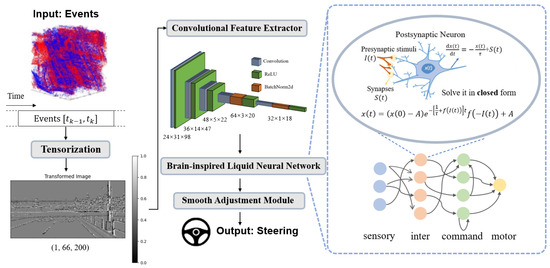
Figure 2.
Overall framework of the proposed LiS-Net. The model includes tensorization, a convolutional feature extractor, a brain-inspired liquid neural network, and a smooth adjustment module. The LiS-Net uses event data as input and predicts the steering angle.
The first step in the framework is tensorization, converting the event streams into tensor form, followed by the use of a convolutional feature extractor to extract meaningful spatial feature representations. Next, the brain-inspired liquid neural network processes the sequential dynamics of the data, focusing on time-series modeling to extract causal relationships. Finally, by incorporating loss design, the framework performs smooth adjustments to produce more stable and refined steering control outputs.
To facilitate understanding of the proposed model and its derivations, we summarize the key symbols and notations used throughout the paper in Table 1.

Table 1.
Summary of key notations used in this paper.
3.1. Data Distribution
The primary objective of this study is to investigate the robustness of brain-inspired networks in processing event-based sensor inputs, with a specific focus on predicting the steering angle for autonomous vehicles. Event-based cameras are particularly appealing for real-time autonomous driving applications due to their high temporal resolution and low latency. However, the availability of real-world autonomous driving datasets incorporating event-based cameras remains limited. To address this challenge, as depicted in Figure 3, the study utilizes EventScape [48], a simulated dataset generated using the CARLA simulator, which provides event camera data for training, validation, and testing purposes. It is important to highlight that the EventScape dataset does not account for variations in weather conditions, with all data collected under clear weather scenarios. Moreover, we qualitatively assess the feasibility and generalization capability of our model using a real-world dataset collected under realistic driving conditions.
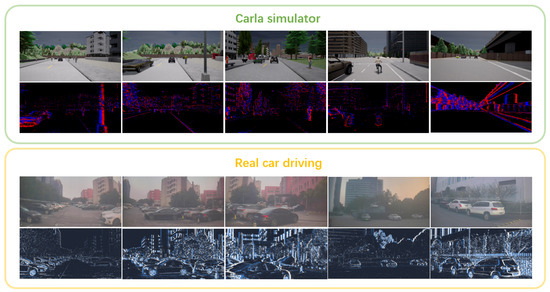
Figure 3.
This figure illustrates the overall data distribution in our study. The model undergoes a complete training, validation, and testing process using the EventScape dataset [48], which is collected using the Carla simulator. In the upper part of the figure, the left three columns show examples selected from the training set, while the right columns display examples from the validation and test sets, respectively. Additionally, our model is validated on a real-world dataset collected during driving experiments with event cameras mounted on a real car. The bottom part of the figure showcases examples selected from sequences in the real-world driving data. Adapted with permission from Ref. [48]. © 2021, the EventScape Dataset authors, released under the GNU General Public License v3.0.
As shown in Figure 4, the real-world dataset in this study consists of data collected from a forward-facing event camera mounted on the roof rack of a vehicle. The vehicle was driven manually by a professional driver, ensuring precise control during data collection. During the data acquisition process, both the environmental data captured by the event camera and the corresponding control signals (e.g., steering angles and vehicle speed) were recorded concurrently. The control signals, obtained from the vehicle’s control system, serve as the ground truth for evaluating the accuracy of the model’s predictions. Similar to the EventScape dataset, the real-world data used for testing was also recorded under clear weather conditions, ensuring consistency with the simulated training data. This approach allows for a thorough assessment of the model’s robustness and its ability to generalize from simulated environments to real-world scenarios.
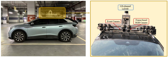
Figure 4.
This figure shows the data collection platform used in this study. As depicted in the diagram, the vehicle is equipped with multiple sensors mounted on the roof rack, including a 128-channel LiDAR, event cameras, and frame-based RGB cameras.
Both the simulated data (EventScape) and real-world data were collected in urban environments, containing typical urban features such as vehicles, pedestrians, and roads. However, the real-world data were specifically captured in a parking lot, ensuring controlled conditions during data collection. To ensure the quality and consistency of the data, the vehicle followed a predefined route, and the data were collected over multiple passes. Additionally, to verify the accuracy and reliability of the collected data, we cross-referenced the event camera data with visual data captured by an RGB camera at corresponding time points. The steering angles at these time points were also manually confirmed to ensure the authenticity and reliability of the data.
3.2. Brain-Inspired Liquid Neural Network
Our approach leverages a brain-inspired liquid neural network to process features extracted from the convolutional layer for autonomous vehicle steering angle prediction. A brain-inspired liquid neural network can be divided into two components: the neuron model and the hierarchical network topology. The neuron model defines the internal structure and mathematical principles for modeling and solving individual neurons, and the hierarchical network topology determines how neurons are organized and connected, including the layering structure and specialized connection mechanisms between different layers. The design of these two components aims to achieve a more sparse and efficient model.
3.2.1. Neuron Model
As is defined by [46], the Liquid Time Constant (LTC) network models the behavior of neurons and synapses as a continuous-time differentiable dynamical system. The dynamics of each neuron i in the LTC network are governed by the following Ordinary Differential Equation (ODE):
where represents the hidden state of neuron i at time t, represents the time constant of neuron i, controlling the rate of state decay, and represents the synaptic input from neuron j to neuron i, given by a nonlinear synaptic function.
To provide a more specific formulation, consider a set of LTC neurons, each with state dynamics , connected through an input synapse to a neuron j:
where represents the time constant of neuron i, where is the leakage conductance and is the membrane capacitance; represents the synaptic weight from neuron i to j; represents the nonlinear activation function; represents the resting potential of neuron i; and represents the reversal synaptic potential defining the polarity of the synapse.
The overall coupling sensitivity (time constant) of the LTC neuron is defined as follows:
Although the Liquid Time Constant (LTC) model effectively simulates the mechanisms of a neuron, it suffers from the excessive computational time required to solve an ordinary differential equation (ODE). To address this issue, closed-form continuous-time (CfC) models [49] are derived from the scalar closed-form solution of the Liquid Time Constant (LTC) system. The hidden state of an LTC network is determined by the solution of the following initial value problem (IVP):
where represents the hidden state of the LTC layer with D cells at time t, represents the exogenous input with m features, represents the time-constant parameter vector, represents the bias vector, f represents a neural network parameterized by , and ⊙ represents the Hadamard (element-wise) product.
The dependence of on allows for the presence of recurrent connections in the system. CfCs address continuous-time dynamics explicitly while maintaining trainability and integration into modern neural network frameworks. The closed-form solution provides a theoretical foundation for solving scalar ordinary differential equation (ODE) systems and ensures well-behaved gradients during optimization.
Given an LTC system defined by an initial value problem (IVP) receiving a single-dimensional time-series input with no self-connections, the approximate closed-form solution is as follows:
Here, represents the initial state of the system, A represents a bias-like parameter, represents the weighted time constant of the neuron, and represents the input-dependent nonlinearity parameterized by .
Since the CfC model is inherently a time-sequence model, one can perform predictions based on an entire sequence of observations. As shown in Table 2, when comparing CfC with other state-of-the-art time-sequence models in terms of time complexity, for a given sequence of length n and a neural network with k hidden units (p being the order of the ODE solver), we observe that the complexity of the ODE-based networks and transformer is at least an order of magnitude higher than that of discrete RNNs and CfCs in both sequence prediction and auto-regressive modeling (time-step prediction) frameworks [49]. This indicates that using CfC as our neuron model can significantly enhance the computational efficiency of the overall network.
Table 2.
Computational complexity of different models.
Considering both computational efficiency and accuracy, we adopt the approximate closed-form solution, as shown in Equation (5), as the neuron model in our brain-inspired liquid neural network.
3.2.2. Hierarchical Network Topology
Neural Circuit Policies (NCPs) [7] are inspired by the wiring diagram of the C. elegans nematode, which features a four-layer hierarchical network topology: sensory neurons, interneurons, command neurons, and motor neurons. As illustrated in the right block of Figure 2, this structure allows for sparse, efficient, and distributed control with hierarchical temporal dynamics. NCPs leverage the specific connectivity patterns found in C. elegans, including feedforward connections (from sensory to intermediate neurons and command to motor neurons) and recurrent connections (within interneurons and command neurons). This topology results in compact networks with around 90% sparsity.
3.2.3. Module Implementation
In the final LiS-Net, we adopt the CfC neuron model and connect it in the form of NCP, thus implementing the module as a brain-inspired liquid neural network. Therefore, this module constructs a recurrent neural network using brain-like ODEs, sequentially introducing the input of sequential environmental dynamics into the CfC model. NCPs are used to sparsify the CfC model, enhancing the network’s efficiency and outputting sequence-controlled actions.
In our hierarchical network topology, the final layer, referred to as the motor layer, includes one neuron that outputs the final prediction for the steering angle. This neuron generates the steering angle prediction based on the processed sequential dynamics, effectively linking the network’s decision-making process to the control action of the vehicle. The detailed network topology parameters are as follows:
- inter_neurons: 22 (Number of interneurons in the network)
- command_neurons: 12 (Number of command neurons used for decision-making)
- motor_neurons: 1 (Number of motor neurons, responsible for outputting the final action)
3.3. Loss Module
The training process uses a custom loss function, which combines two components: an imitation loss and a smoothness loss. The total loss ensures accurate prediction of the steering angle while encouraging smooth transitions between consecutive predictions. The total loss is defined as:
where represents the imitation loss that measures the error between the predicted steering angle and the expert steering angle , represents the smoothness loss that encourages gradual changes in the steering angles over time, and w represents a hyperparameter (smooth_weight) that controls the relative importance of the smoothness loss. The value of w is determined by ablation experiments, which show that a value of w = 1 typically yields the best performance based on our current experiments.
3.3.1. Imitation Loss
The imitation loss is implemented as the Mean Squared Error (MSE) between the predicted steering angle and the expert steering angle. It ensures that the model accurately mimics the expert’s behavior. The imitation loss is given as follows:
where N is the total number of samples in the batch.
3.3.2. Smoothness Loss
The smoothness loss penalizes large changes in the steering angles between consecutive time steps to ensure gradual and smooth transitions. It is calculated as the mean squared difference between consecutive predictions along the time sequence:
where T is the total number of time steps in the sequence.
4. Experiments and Results
4.1. Datasets
As introduced in Section 3.1, our task involves training and testing the model on a simulated dataset and deploying it on real-world data to evaluate its performance. This section focuses on the data-related work.
4.1.1. Our Self-Collected Dataset
We used the experimental vehicle platform developed by Volkswagen (Volkswagen AG, Wolfsburg, Germany), equipped with multiple modality and surround sensors, including a 128-channel Ouster LiDAR sensor, RGB frame sensors, and Prophesee event cameras. The experiments were conducted in Shanghai, China. The proposed method used CAN bus data and event data in this study. We utilized only a single forward-facing event camera with a resolution of 1280 × 720 pixels. The vehicle was also equipped with a drive-by-wire system to collect real CAN bus data, which include torque, speed, throttle, brake, and steering angle. Both the sensor data and CAN data were timestamped during collection, and time synchronization between the two data streams was performed based on absolute time.
Since the event camera has an extremely high temporal resolution, allowing for a very high sampling frequency, we aligned the data to the CAN data’s sampling frequency, which was set to 50 Hz. The entire process of data collection, temporal and spatial synchronization, and data decoding was managed by dedicated built-in software, with specific details omitted here for brevity. In this experiment, to validate the performance of our model, we collected 2 min of data for verification. We will release the processed dataset, ready for deployment, to the research community.
4.1.2. Simulated Dataset
EventScape [48] is a large-scale synthetic dataset designed for multimodal learning tasks, recorded using the CARLA simulator [50]. It contains a total of 743 driving sequences with 171,000 labeled frames, equivalent to approximately 2 h of driving data. EventScape includes diverse automotive scenarios, featuring dynamic actors such as pedestrians and vehicles, making it suitable for developing pedestrian-aware perception algorithms.
The dataset provides a variety of modalities, including events, RGB frames, semantic labels, depth maps, and vehicle signals (e.g., position, orientation, velocity, steering angle, throttle, and brake). Events are generated at 500 Hz using the ESIM simulator, while frames, depth, and semantic labels are synchronized and provided at 25 Hz. Vehicle control data are recorded at 1000 Hz. Events are processed to include realistic features such as a refractory period (100 µs) to resemble real event camera behavior.
Since our model uses only event inputs, we established event–control pairs at 500 Hz by matching each steering angle to its temporally nearest event using timestamp-based nearest-neighbor interpolation. This approach preserves the high temporal resolution of event data while maintaining synchronization with control signals.
EventScape is originally split into training (536 sequences, 71 GB), validation (103 sequences, 12 GB), and test sets (119 sequences, 14 GB). This corresponds approximately to a 70%/15%/15% split, which is commonly adopted in deep learning tasks based on this dataset [48]. Training data are drawn from CARLA towns 1, 2, and 3, while validation and test data come from geographically distinct areas in town 5, ensuring no overlap. In our task, we also followed this split to conduct training, validation, and testing accordingly.
4.1.3. Preprocessing of Event Data
When working with event-based data, one of the key challenges is how to structure and represent the data in a format suitable for training neural networks, particularly in the context of sequential data. In this process, tensorization is a critical step. Specifically, histogram-based tensorization is a widely used method to efficiently convert event streams into structured data formats that can be processed by neural networks, including Convolutional Neural Networks (CNNs) and Recurrent Neural Networks (RNNs).
The histogram method involves discretizing event data into cells based on the spatial coordinates (x,y) of the events, with each cell representing a pixel or region in the spatial grid. Events are then assigned to specific time bins according to their timestamp t. For each time bin, the number of events in each spatial cell is counted, with separate counts for each polarity (ON and OFF), resulting in two distinct channels in the final tensor. The histogram values represent the number of events in each spatial cell for a given time bin, categorized by their polarity. Let H be a tensor of four dimensions . For each event , we update the histogram of the corresponding time bin accordingly:
where is the time interval in microseconds.
After tensorization, the simulated dataset can be directly cropped to the required size and fed into the network for training, as it typically has lower resolution and minimal noise. However, for our collected dataset, the event camera sensor features a higher pixel resolution, requiring additional preprocessing steps to adapt to the network model. As shown in the Figure 5, the resolution is first downsampled from 1280 × 720 pixels to 640 × 360 pixels. Due to noise and an excessive number of event points during data collection, further filtering is applied to filter outliers. This process involves calculating the mean () and standard deviation () of the data and defining thresholds based on a specified number of standard deviations ().
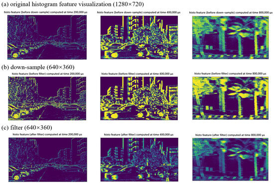
Figure 5.
Preprocess of our collected dataset. (a) Visualization of the original tensor. (b) Visualization of the tensor after down-sampling. (c) Visualization of the tensor after filtering out outliers. From left to right, the images represent different time points: the leftmost shows the car moving straight at a slow speed, the middle shows the car making a slow turn, and the rightmost shows the car making a sharp turn at a high speed.
The number of standard deviations (num_std) used in the Hampel filter was empirically selected based on the distribution of data in our collected dataset. In our experiments, we found that using num_std = 3 yielded optimal performance, effectively filtering outliers without removing valid data points. Specifically, values outside the range
were considered outliers. These outliers were then clipped, resulting in a normalized dataset free of extreme values, ensuring improved data quality for further processing.
It is important to note that the tensorization and preprocessing procedures were consistent across both our model and all baseline models. This uniformity ensures a fair and unbiased comparison of model performance.
4.2. Baseline
To explore the suitability of brain-inspired networks for event-based inputs, we conducted experiments to evaluate the impact of incorporating brain-inspired architectures. Specifically, we compared traditional networks with brain-inspired networks to analyze their performance in the context of event-based data processing for end-to-end steering prediction.
For traditional networks, we selected several traditional neural networks for comparison, including:
(1) CNN (Convolutional Neural Network): A classical convolutional architecture for spatial feature extraction. (2) LSTM (Long Short-Term Memory): A recurrent network capable of capturing temporal dependencies in sequential data. (3) CT-RNN (Continuous-Time Recurrent Neural Network): A model that incorporates ODE (ordinary differential equation) computations to handle irregular observations. CT-RNN achieves this by continuously evolving hidden states between observations, using neural ODEs or neural flow layers.
For brain-inspired networks, we selected (4) NCP (Neural Circuit Policies), a model originally designed for frame-based RGB inputs. To adapt it for event-based data, we first tensorized the event camera input and then fed it into the NCP model, using it as one of our baselines.
By comparing the performance of traditional networks (CNN, LSTM, CT-RNN) with the brain-inspired network, we aim to gain insights into the effectiveness of brain-inspired architectures for event-based end-to-end lateral control tasks. The quantitative and qualitative results of this comparison are provided in subsequent sections.
4.3. Training Details
We implemented the proposed LiS-Net network using PyTorch 2.0.0 with CUDA 12.2. The network was trained on a server equipped with two NVIDIA RTX A6000 GPUs (NVIDIA Corporation, Santa Clara, CA, USA) graphics cards. The batch size during training was set to 128. The input to the network, after tensorization of all event camera data, was resized to the same dimensions (1,66,200) before being fed into the network.
The optimizer used for training was the Adam optimizer, configured with a learning rate of , , , , and no weight decay (). The network was trained for 35 epochs.
Two evaluation metrics, the root mean square error (RMSE) and mean absolute error (MAE), were used to evaluate the effectiveness of the proposed network.
Here, k represents the total number of predictions, is the ground truth value, and is the predicted value. These metrics were used to quantitatively assess the performance of the network.
4.4. Results
4.4.1. Model Efficiency
Quantitative and qualitative analyses were performed to evaluate both the predictive performance and computational efficiency of the proposed method, particularly on the CARLA-based EventScape dataset. As a first step, we examined the loss curves for all models during both the training and validation phases to visually assess their behavior. As illustrated in Figure 6, the loss curves for all models are presented. To ensure a fair comparison, only the MSE loss is considered. From the figure, it can be seen that LiS-Net reaches the minimum loss during the final stage of stabilization, suggesting its efficient training and prediction performance.
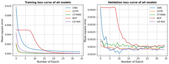
Figure 6.
Loss comparison of different models. Since all baseline models use MSE as their loss function, and LiS-Net additionally incorporates a smooth loss, for the sake of a fair comparison, only the MSE loss is calculated and reported here.
In the context of steering angle prediction, two key metrics were used: Root Mean Square Error (RMSE) and Mean Absolute Error (MAE). Higher RMSE values indicate the presence of large, infrequent deviations in steering angle predictions, potentially leading to instability in vehicle control. MAE reflects the average magnitude of prediction errors and provides insight into overall prediction accuracy. As shown in Table 3, we report RMSE, MAE, the number of model neurons (as a proxy for parameter count), and floating-point operations (FLOPs), which offer a direct measure of computational complexity during inference.
Table 3.
Metric comparison of different models for the EventScape dataset.
To provide a more comprehensive perspective on model efficiency, we additionally calculate the FLOPs required by each network at different sequence lengths (Seq = 1 and Seq = 16). The results indicate that brain-inspired models such as NCP and LiS-Net exhibit lower FLOPs compared to conventional architectures like CNN and LSTM. Among them, NCP achieves the lowest computational cost, while LiS-Net remains highly competitive, achieving comparable efficiency with only a marginal increase in FLOPs. Notably, LiS-Net attains the best overall predictive accuracy, with the lowest RMSE and MAE scores across all evaluated models.
These results highlight the strength of LiS-Net in balancing accuracy and efficiency. By leveraging the compact structure of neural circuit policies and the dynamic temporal modeling capability of CfC neurons, LiS-Net demonstrates strong potential for real-time deployment in resource-constrained autonomous systems.
To further evaluate the performance of different models on event data, a qualitative comparison of steering angle prediction using various frameworks, including CNN, NCP, and LiS-Net, was performed. The results are illustrated in Figure 7, where the left graph shows a comparison of predictions across the entire test dataset, the middle graph presents a zoomed-in segment for closer analysis, and the right graph illustrates the deployment results on our collected dataset.
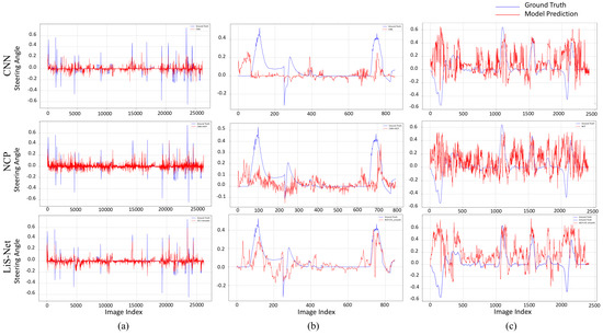
Figure 7.
A qualitative comparison among different models. (a) Steering angle prediction with all EventSacpe test dataset. (b) Steering angle prediction with selected EventSacpe test dataset. (c) Steering angle prediction with our collected dataset.
As shown in Figure 7, the brain-inspired networks outperformed the CNN in terms of fitting the amplitude of the steering angles more accurately. However, the predictions from the NCP model exhibited noticeable oscillations, which can affect stability. In contrast, LiS-Net, with its incorporation of a smooth adjustment mechanism, achieved significantly better overall smoothness in the predictions while maintaining a high degree of accuracy in amplitude fitting. This demonstrates the advantage of LiS-Net in achieving both precise and stable steering predictions, making it a robust choice for event-based steering tasks.
4.4.2. Model Generalization
When deploying the above models on an unfamiliar dataset, namely our collected dataset, it is evident from Figure 7 that the accuracy and smoothness of the predictions were not as strong as the results observed during testing on the simulation dataset. However, comparing the models horizontally, our proposed LiS-Net demonstrates superior performance, particularly in terms of maintaining smooth predictions. To quantify smoothness, we computed the total variation () of the steering angle predictions. The total variation was 105.42 for the CNN, 130.08 for NCP, and 94.93 for LiS-Net. Clearly, LiS-Net achieved the lowest total variation, indicating significantly smoother predictions compared to the other models. This highlights the robustness and generalizability of LiS-Net, making it better suited for real-world deployment and diverse scenarios.
In discussing Figure 7c, we note the two downfacing spikes in the ground truth data (in blue). Actually, these spikes occur at intersections where both left and right turns are feasible. However, the overall route design specifies right turns at these locations, meaning the ground truth reflects right-turn trajectories. The observed downfacing spikes may result from a mismatch between the simulated training data, which likely contained more left-turn intersections, and the real-world route, which requires right turns. Consequently, the models predict left turns at these points, not due to model failure but to the data distribution in the simulation. This suggests that the discrepancy is rooted in the nature of the training data rather than the model’s generalization capability.
4.5. Ablation Studies
To further investigate the efficacy of the proposed method, we conducted ablation studies focusing on the design of the loss function and the contribution of individual model components. As shown in Figure 8, we designed two sets of ablation experiments to support our findings.
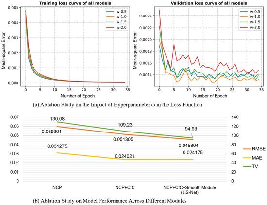
Figure 8.
Ablation studies on the proposed method. (a) Effect of varying the smoothness weight w in the loss function. Setting achieves the best trade-off between imitation accuracy and output smoothness. (b) Evaluation of the effectiveness of different components in LiS-Net compared to the NCP baseline, using RMSE and MAE (for accuracy) and TV (for smoothness). Both the CfC-based neuron model and the smooth adjustment module contribute significantly to overall performance improvement.
4.5.1. Ablation Study on the Impact of Hyperparameter w in the Loss Function
As previously mentioned, our loss function consists of two components: imitation loss and smoothness loss. The hyperparameter w determines the relative weight between these two terms, and choosing an appropriate value for w is crucial to achieving a balance between prediction accuracy and output smoothness.
This experiment visualizes the training and validation performance under different values of the weight w assigned to the smoothness term. The results show that setting achieves the best trade-off between the imitation loss and the smoothness loss, leading to optimal overall performance. This demonstrates the importance of carefully balancing accuracy and smoothness during training.
4.5.2. Ablation Study on Model Performance Across Different Modules
This analysis evaluates the contribution of different components within our LiS-Net architecture by comparing it against the baseline NCP model using three metrics: RMSE and MAE for accuracy, and Total Variation (TV) for smoothness. The experimental results confirm that integrating the CfC-based neuron model and the proposed smooth adjustment module significantly improves both accuracy and smoothness. These components are thus essential for achieving the overall performance gains observed in LiS-Net.
5. Discussion
5.1. Advantages of Brain-Inspired Networks over Traditional Models
While our experimental results demonstrate that LiS-Net outperforms traditional CNN and LSTM models in steering angle prediction, it is crucial to further explain the underlying reasons. Brain-inspired networks, such as the NCP-based architecture employed in LiS-Net, exhibit several properties that contribute to this superior performance:
- Temporal dynamics and causal representation: Unlike traditional models that often rely on static or fixed-window temporal features, the neuron models used in NCPs (and extended in LiS-Net) are capable of capturing fine-grained temporal dependencies and causal relationships. This allows the model to better understand and predict driving behaviors, especially in continuous control tasks.
- Compactness and interpretability: LiS-Net inherits the structural compactness and sparsity of NCPs, which help reduce overfitting and improve generalization to unseen roads. The internal dynamics are often more interpretable compared to black-box CNN–LSTM hybrids.
- Task specificity and modularity: LiS-Net is designed as a task-specific controller, allowing it to focus computational resources on learning relevant features for steering control. This modularity also supports better integration into full-stack autonomous systems.
Compared to conventional neural architectures, these properties make brain-inspired networks particularly suitable for real-time control tasks in dynamic, uncertain environments.
5.2. Limitations in Smoothness and Practical Control Applications
Although LiS-Net demonstrates improved prediction smoothness through the proposed smooth adjustment module, we acknowledge that prediction smoothness alone does not guarantee smooth control in practical deployment scenarios. In real-world driving, control systems must consider system latency, actuation dynamics, and environmental disturbances. Therefore, integrating post-processing techniques, such as low-pass filtering or control-oriented trajectory smoothing modules, may still be necessary to ensure stable and safe control under dynamic conditions. This highlights the gap between perception-level prediction smoothness and actual control robustness.
5.3. Challenges and Opportunities in Brain-Inspired Models
LiS-Net builds upon the NCP framework by introducing a more computationally efficient neuron model (CfC) and a smooth adjustment module, enhancing both inference speed and output quality. However, brain-inspired networks still face several practical challenges:
- Lack of mature toolchains: Unlike transformer-based models that benefit from well-optimized libraries and hardware-accelerated deployment stacks, brain-inspired architectures lack standardized quantization, acceleration, and deployment tools.
- Hardware compatibility: Current deep learning hardware, especially GPUs, is optimized for dense matrix operations and transformer-style parallelism. Brain-inspired models often have sparse, time-dependent structures that are less compatible with existing hardware, leading to suboptimal runtime performance.
- Need for specialized hardware: To fully realize the theoretical advantages of brain-inspired computation, it may be necessary to co-develop hardware architectures (e.g., neuromorphic chips) that align with these models’ computational paradigms. While this is still in early stages, it represents a promising direction for future research and deployment.
Despite these limitations, we believe brain-inspired models offer an exciting alternative to conventional deep learning in safety-critical and real-time decision-making scenarios, such as autonomous driving. Continued research on optimization, hardware support, and scalable training techniques will be crucial to unlocking their full potential.
6. Conclusions
This paper explores the integration of event cameras with brain-inspired neural networks and proposes a novel architecture called LiS-Net for end-to-end steering angle prediction. By leveraging event cameras as input and combining them with brain-inspired neural networks, LiS-Net shows promising results when compared to traditional networks. Specifically, our approach reduces the number of neurons while achieving improved performance in terms of RMSE and MAE metrics. To evaluate its effectiveness, we trained and tested LiS-Net on a simulated dataset and further validated its performance on a real-world dataset collected using an experimental vehicle equipped with event cameras. The qualitative and quantitative evaluation indicates that LiS-Net consistently outperforms traditional methods, demonstrating reliable and accurate steering angle predictions. These findings suggest that combining bio-inspired sensors with brain-inspired computation could be a viable direction for more scalable and efficient autonomous driving solutions.
However, this work is limited to steering angle prediction, and further research is needed to extend the application of brain-inspired networks to longitudinal control tasks, such as velocity prediction or braking control. Additionally, our current study uses event cameras as the sole input modality. Event cameras offer significant advantages, such as high temporal resolution and robustness to dynamic lighting conditions, which are particularly useful for handling high-speed motion and fast-changing environments. However, event cameras also have certain limitations, such as the lack of detailed intensity information and lower spatial resolution compared to frame-based cameras.
Given these strengths and limitations, future research could explore the fusion of event cameras with frame-based cameras to capitalize on their complementary advantages. While event cameras excel at capturing fast-moving objects and providing detailed temporal information, frame-based cameras can offer rich spatial details and color information. By combining these modalities, future systems could achieve a more comprehensive understanding of the environment, leading to improved perception and decision-making capabilities for autonomous driving applications.
Author Contributions
Conceptualization, K.X., E.C., F.Z. and M.L.; Methodology, K.X., J.L., S.W. and E.C.; Software, K.X.; Validation, K.X. and J.L.; Investigation, K.X., J.L. and S.W.; Resources, F.Z. and M.L.; Data curation, J.L.; Writing—original draft, K.X.; Writing—review & editing, J.L. and M.L.; Supervision, M.L.; Project administration, M.L.; Funding acquisition, F.Z. and M.L. All authors have read and agreed to the published version of the manuscript.
Funding
The following funding sources provided to M.L. are acknowledged: the National Natural Science Foundation of China (32371083) and the National Key Research and Development Program of China (2021YFF1200700 & 2021YFC2501500). The funders had no role in study design, data collection, analysis, decision to publish, or preparation of the manuscript.
Data Availability Statement
The data presented in this study are openly available in LiS-Net at https://github.com/CocoYi-Claire/LiS-Net, accessed on 25 April 2025.
Conflicts of Interest
Author Erkang Cheng was employed by the company NullMax. Author Fang Zhao was employed by the company DiFint Technology and INSIDE Institute for Biological and Artificial Intelligence. The remaining authors declare that the research was conducted in the absence of any commercial or financial relationships that could be construed as a potential conflict of interest.
Appendix A
Table A1.
Convolutional head used in LiS-Net. Size of the convolutional kernels.
Table A1.
Convolutional head used in LiS-Net. Size of the convolutional kernels.
| Layer | Filter | Kernel Size | Stride |
|---|---|---|---|
| 1 | 24 | 5 | 2 |
| 2 | 36 | 5 | 2 |
| 3 | 48 | 3 | 2 |
| 4 | 64 | 3 | 1 |
| 5 | 8 | 3 | 1 |
Table A2.
Model architecture overview.
Table A2.
Model architecture overview.
| Model | Layers | Loss | Train Time per Epoch (min) |
|---|---|---|---|
| CNN | Conv2d ×5, ReLU ×5, Linear ×4, Dropout ×3 | MSELoss | 5.93 |
| LSTM | Conv2d ×5, ReLU ×5, LSTM, Linear ×1 | MSELoss | 93.39 |
| CT-RNN | Conv2d ×5, ReLU ×5, Linear ×35, Softmax ×2, Tanh ×1 | MSELoss | 116.92 |
| NCP | Conv2d ×5, ReLU ×5, Linear ×1, LTCCell ×3 | MSELoss | 87.84 |
| LiS-Net | Conv2d ×5, ReLU ×5, Linear ×1, WiredCfCCell ×3 | MSELoss + SmoothLoss | 72.71 |
Table A3.
CNN model architecture.
Table A3.
CNN model architecture.
| Layer Name | Type | Input Shape | Output Shape |
|---|---|---|---|
| Conv1 | Conv2d | ||
| ReLU | |||
| Conv2 | Conv2d | ||
| ReLU | |||
| Conv3 | Conv2d | ||
| ReLU | |||
| Conv4 | Conv2d | ||
| ReLU | |||
| Conv5 | Conv2d | ||
| ReLU | |||
| Dropout1 | Dropout | ||
| Dropout2 | Dropout | ||
| Dropout3 | Dropout | ||
| Linear1 | Linear | ||
| Linear2 | Linear | ||
| Linear3 | Linear | ||
| Linear4 | Linear |
Table A4.
LSTM model architecture.
Table A4.
LSTM model architecture.
| Layer Name | Type | Input Shape | Output Shape |
|---|---|---|---|
| Convolutional Head | Conv2d | ||
| ReLU | |||
| Conv2d | |||
| ReLU | |||
| Conv2d | |||
| ReLU | |||
| Conv2d | |||
| BatchNorm2d | |||
| ReLU | |||
| Conv2d | |||
| BatchNorm2d | |||
| ReLU | |||
| Linear layers (1 to 32) | Linear | (4416) | (128) |
| LSTM Output Layer | LSTM | ||
| Linear |
Table A5.
CT-RNN model architecture.
Table A5.
CT-RNN model architecture.
| Layer Name | Type | Input Shape | Output Shape |
|---|---|---|---|
| Conv1 | Conv2d | ||
| ReLU | |||
| Conv2 | Conv2d | ||
| ReLU | |||
| Conv3 | Conv2d | ||
| ReLU | |||
| Conv4 | Conv2d | ||
| ReLU | |||
| Conv5 | Conv2d | ||
| ReLU | |||
| BatchNorm1 | BatchNorm2d | ||
| Dropout1 | Dropout | ||
| Linear Layers (1 to 32) | Linear | (608) | (144) |
| Linear_r | Linear | ||
| Linear_q | Linear | ||
| Linear_s | Linear | ||
| Softmax_r | Softmax | ||
| Softmax_s | Softmax | ||
| Tanh | Tanh |
Table A6.
NCP model architecture.
Table A6.
NCP model architecture.
| Layer Name | Type | Input Shape | Output Shape |
|---|---|---|---|
| Conv1 | Conv2d | (1, 66, 200) | (24, 31, 98) |
| ReLU | (24, 31, 98) | (24, 31, 98) | |
| Conv2 | Conv2d | (24, 31, 98) | (36, 14, 47) |
| ReLU | (36, 14, 47) | (36, 14, 47) | |
| Conv3 | Conv2d | (36, 14, 47) | (48, 5, 22) |
| ReLU | (48, 5, 22) | (48, 5, 22) | |
| Conv4 | Conv2d | (48, 5, 22) | (64, 3, 20) |
| BatchNorm2d | (64, 3, 20) | (64, 3, 20) | |
| ReLU | (64, 3, 20) | (64, 3, 20) | |
| Conv5 | Conv2d | (64, 3, 20) | (32, 1, 18) |
| BatchNorm2d | (32, 1, 18) | (32, 1, 18) | |
| ReLU | (32, 1, 18) | (32, 1, 18) | |
| Linear Layers (1 to 32) | Linear | (576) | (32) |
| LTCCell Layers | LTCCell | (32) | (22) |
| LTCCell | (22) | (12) | |
| LTCCell | (12) | (1) |
Table A7.
LiS-Net architecture.
Table A7.
LiS-Net architecture.
| Layer Name | Type | Input Shape | Output Shape |
|---|---|---|---|
| Conv1 | Conv2d | (1, 66, 200) | (24, 31, 98) |
| ReLU | (24, 31, 98) | (24, 31, 98) | |
| Conv2 | Conv2d | (24, 31, 98) | (36, 14, 47) |
| ReLU | (36, 14, 47) | (36, 14, 47) | |
| Conv3 | Conv2d | (36, 14, 47) | (48, 5, 22) |
| ReLU | (48, 5, 22) | (48, 5, 22) | |
| Conv4 | Conv2d | (48, 5, 22) | (64, 3, 20) |
| BatchNorm2d | (64, 3, 20) | (64, 3, 20) | |
| ReLU | (64, 3, 20) | (64, 3, 20) | |
| Conv5 | Conv2d | (64, 3, 20) | (32, 1, 18) |
| BatchNorm2d | (32, 1, 18) | (32, 1, 18) | |
| ReLU | (32, 1, 18) | (32, 1, 18) | |
| Linear Layers (1 to 32) | Linear | (576) | (32) |
| WiredCfCCell1 | Layer 0 (ff1) | (32) | (22) |
| Layer 0 (ff2) | (22) | (22) | |
| Layer 0 (time_a) | (22) | (22) | |
| Layer 0 (time_b) | (22) | (22) | |
| WiredCfCCell2 | Layer 1 (ff1) | (22) | (12) |
| Layer 1 (ff2) | (12) | (12) | |
| Layer 1 (time_a) | (12) | (12) | |
| Layer 1 (time_b) | (12) | (12) | |
| WiredCfCCell3 | Layer 2 (ff1) | (12) | (1) |
| Layer 2 (ff2) | (1) | (1) | |
| Layer 2 (time_a) | (1) | (1) | |
| Layer 2 (time_b) | (1) | (1) |
References
- Azam, S.; Munir, F.; Sheri, A.M.; Kim, J.; Jeon, M. System, design and experimental validation of autonomous vehicle in an unconstrained environment. Sensors 2020, 20, 5999. [Google Scholar] [CrossRef]
- Saleem, H.; Riaz, F.; Mostarda, L.; Niazi, M.A.; Rafiq, A.; Saeed, S. Steering angle prediction techniques for autonomous ground vehicles: A review. IEEE Access 2021, 9, 78567–78585. [Google Scholar] [CrossRef]
- Gallego, G.; Delbrück, T.; Orchard, G.; Bartolozzi, C.; Taba, B.; Censi, A.; Leutenegger, S.; Davison, A.J.; Conradt, J.; Daniilidis, K.; et al. Event-based vision: A survey. IEEE Trans. Pattern Anal. Mach. Intell. 2020, 44, 154–180. [Google Scholar] [CrossRef]
- Posch, C.; Matolin, D.; Wohlgenannt, R. A QVGA 143dB dynamic range asynchronous address-event PWM dynamic image sensor with lossless pixel-level video compression. In Proceedings of the 2010 IEEE International Solid-State Circuits Conference-(ISSCC), San Francisco, CA, USA, 7–11 February 2010; pp. 400–401. [Google Scholar]
- Berner, R.; Brandli, C.; Yang, M.; Liu, S.C.; Delbruck, T. A 240x180 10mW 12us latency sparse-output vision sensor for mobile applications. In Proceedings of the 2013 Symposium on VLSI Circuits, Kyoto, Japan, 12–14 June 2013; pp. C186–C187. [Google Scholar]
- Hu, Y.; Binas, J.; Neil, D.; Liu, S.C.; Delbruck, T. Ddd20 end-to-end event camera driving dataset: Fusing frames and events with deep learning for improved steering prediction. In Proceedings of the 2020 IEEE 23rd International Conference on Intelligent Transportation Systems (ITSC), Rhodes, Greece, 20–23 September 2020; pp. 1–6. [Google Scholar]
- Lechner, M.; Hasani, R.; Amini, A.; Henzinger, T.A.; Rus, D.; Grosu, R. Neural circuit policies enabling auditable autonomy. Nat. Mach. Intell. 2020, 2, 642–652. [Google Scholar] [CrossRef]
- Chen, C.; Seff, A.; Kornhauser, A.; Xiao, J. Deepdriving: Learning affordance for direct perception in autonomous driving. In Proceedings of the IEEE International Conference on Computer Vision, Santiago, Chile, 7–13 December 2015; pp. 2722–2730. [Google Scholar]
- Patil, A.; Malla, S.; Gang, H.; Chen, Y.T. The h3d dataset for full-surround 3d multi-object detection and tracking in crowded urban scenes. In Proceedings of the 2019 International Conference on Robotics and Automation ICRA, Montreal, QC, Canada, 20–24 May 2019; pp. 9552–9557. [Google Scholar]
- Akai, N.; Morales, L.Y.; Yamaguchi, T.; Takeuchi, E.; Yoshihara, Y.; Okuda, H.; Suzuki, T.; Ninomiya, Y. Autonomous driving based on accurate localization using multilayer LiDAR and dead reckoning. In Proceedings of the 2017 IEEE 20th International Conference on Intelligent Transportation Systems (ITSC), Kanagawa, Japan, 16–19 October 2017; pp. 1–6. [Google Scholar]
- Song, H.; Luan, D.; Ding, W.; Wang, M.Y.; Chen, Q. Learning to predict vehicle trajectories with model-based planning. In Proceedings of the Conference on Robot Learning, CoRL, London, UK, 8–11 November 2021; pp. 1035–1045. [Google Scholar]
- Pomerleau, D.A. Alvinn: An autonomous land vehicle in a neural network. Adv. Neural Inf. Process. Syst. 1988, 305–313. [Google Scholar]
- Chen, D.; Zhou, B.; Koltun, V.; Krähenbühl, P. Learning by cheating. In Proceedings of the Conference on Robot Learning, PMLR, London, UK, 16–18 November 2020; pp. 66–75. [Google Scholar]
- Ohn-Bar, E.; Prakash, A.; Behl, A.; Chitta, K.; Geiger, A. Learning situational driving. In Proceedings of the IEEE/CVF Conference on Computer Vision and Pattern Recognition, Seattle, WA, USA, 16–18 June 2020; pp. 11296–11305. [Google Scholar]
- Zhao, A.; He, T.; Liang, Y.; Huang, H.; Van den Broeck, G.; Soatto, S. Sam: Squeeze-and-mimic networks for conditional visual driving policy learning. In Proceedings of the 2020 Conference on Robot Learning, CoRL, London, UK, 16–18 November 2020; pp. 156–175. [Google Scholar]
- Hanselmann, N.; Renz, K.; Chitta, K.; Bhattacharyya, A.; Geiger, A. King: Generating safety-critical driving scenarios for robust imitation via kinematics gradients. In Proceedings of the European Conference on Computer Vision, Tel Aviv, Israel, 23–24 October 2022; Springer: Cham, Switzerland, 2022; pp. 335–352. [Google Scholar]
- Chitta, K.; Prakash, A.; Jaeger, B.; Yu, Z.; Renz, K.; Geiger, A. Transfuser: Imitation with transformer-based sensor fusion for autonomous driving. IEEE Trans. Pattern Anal. Mach. Intell. 2022, 45, 12878–12895. [Google Scholar] [CrossRef]
- Chen, D.; Krähenbühl, P. Learning from all vehicles. In Proceedings of the IEEE/CVF Conference on Computer Vision and Pattern Recognition, New Orleans, LA, USA, 18–24 June 2022; pp. 17222–17231. [Google Scholar]
- Codevilla, F.; Santana, E.; López, A.M.; Gaidon, A. Exploring the limitations of behavior cloning for autonomous driving. In Proceedings of the IEEE/CVF International Conference on Computer Vision, Seoul, Republic of Korea, 27 October–2 November 2019; pp. 9329–9338. [Google Scholar]
- Chib, P.S.; Singh, P. Recent advancements in end-to-end autonomous driving using deep learning: A survey. IEEE Trans. Intell. Veh. 2023, 9, 103–118. [Google Scholar] [CrossRef]
- Toromanoff, M.; Wirbel, E.; Moutarde, F. End-to-end model-free reinforcement learning for urban driving using implicit affordances. In Proceedings of the IEEE/CVF Conference on Computer Vision and Pattern Recognition, Seattle, WA, USA, 16–18 June 2020; pp. 7153–7162. [Google Scholar]
- Li, Q.; Peng, Z.; Zhou, B. Efficient learning of safe driving policy via human-ai copilot optimization. arXiv 2022, arXiv:2202.10341. [Google Scholar]
- Bojarski, M.; Choromanska, A.; Choromanski, K.; Firner, B.; Jackel, L.; Muller, U.; Zieba, K. Visualbackprop: Visualizing cnns for autonomous driving. arXiv 2016, arXiv:1611.05418. [Google Scholar]
- Karsli, M.; Satilmiş, Y.; Şara, M.; Tufan, F.; Eken, S.; Sayar, A. End-to-end learning model design for steering autonomous vehicle. In Proceedings of the 2018 26th Signal processing and communications applications conference (SIU), Izmir, Turkey, 2–5 May 2018; pp. 1–4. [Google Scholar]
- Xu, H.; Gao, Y.; Yu, F.; Darrell, T. End-to-end learning of driving models from large-scale video datasets. In Proceedings of the IEEE Conference on Computer Vision and Pattern Recognition, Honolulu, HI, USA, 21–26 July 2017; pp. 2174–2182. [Google Scholar]
- Kim, J.; Canny, J. Interpretable learning for self-driving cars by visualizing causal attention. In Proceedings of the IEEE International Conference on Computer Vision, Venice, Italy, 22–29 October 2017; pp. 2942–2950. [Google Scholar]
- Azam, S.; Munir, F.; Rafique, M.A.; Sheri, A.M.; Hussain, M.I.; Jeon, M. N 2 C: Neural network controller design using behavioral cloning. IEEE Trans. Intell. Transp. Syst. 2021, 22, 4744–4756. [Google Scholar] [CrossRef]
- Xie, Q.; Long, Q.; Li, J.; Zhang, L.; Hu, X. Application of intelligence binocular vision sensor: Mobility solutions for automotive perception system. IEEE Sens. J. 2023, 24, 5578–5592. [Google Scholar] [CrossRef]
- Xie, Q.; Hu, X.; Ren, L.; Qi, L.; Sun, Z. A binocular vision application in IoT: Realtime trustworthy road condition detection system in passable area. IEEE Trans. Ind. Inform. 2022, 19, 973–983. [Google Scholar] [CrossRef]
- Sobh, I.; Amin, L.; Abdelkarim, S.; Elmadawy, K.; Saeed, M.; Abdeltawab, O.; Gamal, M.; El Sallab, A. End-to-End Multi-Modal Sensors Fusion System for Urban Automated Driving. 2018. Available online: https://openreview.net/pdf?id=Byx4Xkqjcm (accessed on 25 April 2025).
- Khan, Q.; Schön, T.; Wenzel, P. Towards self-supervised high level sensor fusion. arXiv 2019, arXiv:1902.04272. [Google Scholar]
- Lichtsteiner, P.; Delbruck, T. A 64x64 AER logarithmic temporal derivative silicon retina. In Proceedings of the Research in Microelectronics and Electronics, 2005 PhD, Lausanne, Switzerland, 28 July 2005; Volume 2, pp. 202–205. [Google Scholar]
- Lichtsteiner, P.; Posch, C.; Delbruck, T. A 128 × 128 120db 30mw asynchronous vision sensor that responds to relative intensity change. In Proceedings of the 2006 IEEE International Solid State Circuits Conference-Digest of Technical Papers, San Francisco, CA, USA, 6–9 February 2006; pp. 2060–2069. [Google Scholar]
- Serrano-Gotarredona, T.; Linares-Barranco, B. A 128×128 1.5% Contrast Sensitivity 0.9% FPN 3 μs Latency 4 mW Asynchronous Frame-Free Dynamic Vision Sensor Using Transimpedance Preamplifiers. IEEE J. Solid-State Circuits 2013, 48, 827–838. [Google Scholar] [CrossRef]
- Ramesh, B.; Zhang, S.; Lee, Z.W.; Gao, Z.; Orchard, G.; Xiang, C. Long-term object tracking with a moving event camera. In Proceedings of the Bmvc, Newcastle, UK, 3–6 September 2018; p. 241. [Google Scholar]
- Zhang, J.; Dong, B.; Zhang, H.; Ding, J.; Heide, F.; Yin, B.; Yang, X. Spiking transformers for event-based single object tracking. In Proceedings of the IEEE/CVF Conference on Computer Vision and Pattern Recognition, New Orleans, LA, USA, 18–24 June 2022; pp. 8801–8810. [Google Scholar]
- Delbruck, T.; Lang, M. Robotic goalie with 3 ms reaction time at 4% CPU load using event-based dynamic vision sensor. Front. Neurosci. 2013, 7, 223. [Google Scholar] [CrossRef]
- Falanga, D.; Kleber, K.; Scaramuzza, D. Dynamic obstacle avoidance for quadrotors with event cameras. Sci. Robot. 2020, 5, eaaz9712. [Google Scholar] [CrossRef]
- Andreopoulos, A.; Kashyap, H.J.; Nayak, T.K.; Amir, A.; Flickner, M.D. A low power, high throughput, fully event-based stereo system. In Proceedings of the IEEE Conference on Computer Vision and Pattern Recognition, Salt Lake City, UT, USA, 18–22 June 2018; pp. 7532–7542. [Google Scholar]
- Binas, J.; Neil, D.; Liu, S.C.; Delbruck, T. DDD17: End-to-end DAVIS driving dataset. arXiv 2017, arXiv:1711.01458. [Google Scholar]
- Maqueda, A.I.; Loquercio, A.; Gallego, G.; García, N.; Scaramuzza, D. Event-based vision meets deep learning on steering prediction for self-driving cars. In Proceedings of the IEEE Conference on Computer Vision and Pattern Recognition, Salt Lake City, UT, USA, 18–22 June 2018; pp. 5419–5427. [Google Scholar]
- Munir, F.; Azam, S.; Yow, K.C.; Lee, B.G.; Jeon, M. Multimodal fusion for sensorimotor control in steering angle prediction. Eng. Appl. Artif. Intell. 2023, 126, 107087. [Google Scholar] [CrossRef]
- Pascarella, L.; Magno, M. Grayscale and event-based sensor fusion for robust steering prediction for self-driving cars. In Proceedings of the 2023 IEEE Sensors Applications Symposium (SAS), Ottawa, ON, Canada, 18–20 July 2023; pp. 01–06. [Google Scholar]
- Koch, C.; Segev, I. Methods in Neuronal Modeling: From Ions to Networks; MIT Press: Cambridge, MA, USA, 1998. [Google Scholar]
- Kandel, E.R.; Schwartz, J.H.; Jessell, T.M.; Siegelbaum, S.; Hudspeth, A.J.; Mack, S. Principles of Neural Science; McGraw-Hill: New York, NY, USA, 2000; Volume 4. [Google Scholar]
- Hasani, R.; Lechner, M.; Amini, A.; Rus, D.; Grosu, R. Liquid time-constant networks. In Proceedings of the AAAI Conference on Artificial Intelligence, Virtual, 2–9 February 2021; Volume 35, pp. 7657–7666. [Google Scholar]
- Wicks, S.R.; Roehrig, C.J.; Rankin, C.H. A dynamic network simulation of the nematode tap withdrawal circuit: Predictions concerning synaptic function using behavioral criteria. J. Neurosci. 1996, 16, 4017–4031. [Google Scholar] [CrossRef]
- Gehrig, D.; Rüegg, M.; Gehrig, M.; Hidalgo-Carrió, J.; Scaramuzza, D. Combining events and frames using recurrent asynchronous multimodal networks for monocular depth prediction. IEEE Robot. Autom. Lett. 2021, 6, 2822–2829. [Google Scholar] [CrossRef]
- Hasani, R.; Lechner, M.; Amini, A.; Liebenwein, L.; Ray, A.; Tschaikowski, M.; Teschl, G.; Rus, D. Closed-form continuous-time neural networks. Nat. Mach. Intell. 2022, 4, 992–1003. [Google Scholar] [CrossRef]
- Dosovitskiy, A.; Ros, G.; Codevilla, F.; Lopez, A.; Koltun, V. CARLA: An open urban driving simulator. In Proceedings of the Conference on Robot Learning, PMLR, California, CA, USA, 13–15 November 2017; pp. 1–16. [Google Scholar]
Disclaimer/Publisher’s Note: The statements, opinions and data contained in all publications are solely those of the individual author(s) and contributor(s) and not of MDPI and/or the editor(s). MDPI and/or the editor(s) disclaim responsibility for any injury to people or property resulting from any ideas, methods, instructions or products referred to in the content. |
© 2025 by the authors. Licensee MDPI, Basel, Switzerland. This article is an open access article distributed under the terms and conditions of the Creative Commons Attribution (CC BY) license (https://creativecommons.org/licenses/by/4.0/).