Disease Monitoring and Characterization of Feeder Road Network Based on Improved YOLOv11

Abstract

In response to the challenges of the low accuracy and high misdetection and omission rate of disease detection on feeder roads, an improved Rural-YOLO (SAConv-C2f+C2PSA_CAA+MCSAttention+WIOU) disease detection algorithm is proposed in this paper, which is an enhanced target detection framework based on the YOLOv11 architecture, for the identification of common diseases in the complex feeder road environment. The proposed methodology introduces four key innovations: (1) Switchable Atrous Convolution (SAConv) is introduced into the backbone network to enhance multiscale disease feature extraction under occlusion conditions; (2) Multi-Channel and Spatial Attention (MCSAttention) is constructed in the feature fusion process, and the weight distribution of multiscale diseases is adjusted through adaptive weight redistribution. By adjusting the weight distribution, the model’s sensitivity to subtle disease features is improved. To enhance its ability to discriminate between different disease types, Cross Stage Partial with Parallel Spatial Attention and Channel Adaptive Aggregation (C2PSA_CAA) is constructed at the end of the backbone network. (3) To mitigate category imbalance issues, Weighted Intersection over Union loss (WIoU_loss) is introduced, which helps optimize the bounding box regression process in disease detection and improve the detection of relevant diseases. Based on experimental validation, Rural-YOLO demonstrated superior performance with minimal computational overhead. Only 0.7 M additional parameters is required, and an 8.4% improvement in recall and a 7.8% increase in mAP₅₀ were achieved compared to the initial models. The optimized architecture also reduced the model size by 21%. The test results showed that the proposed model achieved 3.28 M parameters with a computational complexity of 5.0 GFLOPs, meeting the requirements for lightweight deployment scenarios. Cross-validation on multi-scenario public datasets was carried out, and the model’s robustness across diverse road conditions. In the quantitative experiments, the center skeleton method and the maximum internal tangent circle method were used to calculate crack width, and the pixel occupancy ratio method was used to assess the area damage degree of potholes and other diseases. The measurements were converted to actual physical dimensions using a calibrated scale of 0.081:1.

1. Introduction

The extensive mileage and widespread distribution of feeder roads necessitate the detection of regular pavement distress. Regular pavement distress detection improves infrastructure longevity and regional economic development. As outlined in the Development Outline for Highway Maintenance and Management During the 14th Five-Year Plan Period, highways in China’s road network, classified as fourth-grade, constitute over 70% of the total road mileage. However, they are disproportionately under-maintained despite their vital role in rural connectivity [1]. This maintenance disparity underscores the urgent need to develop applicable disease detection techniques for lower-tier roads, which is a core objective of this study. The unique challenges associated with pavement disease detection on low-grade feeder roads are illustrated in Figure 1, including multiscale disease variability, occlusion of disease surfaces by shadows or disturbances (e.g., vegetation encroachment and seasonal debris), and the coexistence of multiple diseases, etc. Traditional inspection methods are inadequate to address these multifaceted challenges, especially given the limitations of typical inspection scenarios for feeder roadway distresses.

As illustrated in Figure 1, the surface of the feeder road is affected by light and obscured by the shadows of objects such as leaves on the roadside, which lead to difficulties in recognizing the detection model in detecting pavement distress when faced with a complex image background [2]. It is challenging to detect roadway damage when the roadway surface is complex and uneven. In addition, there are finer disturbances on the surface of feeder roads, such as weeds, tree branches, and soil, which have textures similar to those of the disease, causing the model to miss or misrecognize them when detecting feeder road diseases. Moreover, in the rural road disease detection task, different scales and types of diseases may coexist in the same image, adding complexity to the recognition task. Therefore, a pavement disease detection algorithm with strong anti-interference and multiscale detection ability is essential for feeder road detection.

Traditional pavement inspection methods, exemplified by crack detection frames utilizing multiscale topological representations, primarily focus on describing cracks through manually processed features. This process is inherently time-consuming and cost-intensive. In recent years, intelligent road distress detection has become increasingly prevalent, with manual characterization techniques being progressively supplanted by automated approaches due to their superior timeliness and accuracy. The rapid advancements in deep learning have demonstrated its efficacy in feature extraction, fusion, and classification within target detection frameworks, establishing it as a mainstream methodology for road distress analysis. Wang [3] employed the Mask R-CNN algorithm to achieve automated pavement crack recognition, enhancing model training outcomes through dataset optimization, image pixel refinement, and annotation improvements, thereby achieving higher crack detection accuracy. However, this framework fails to fully account for complex environmental variables, resulting in limited generalization capability under varying lighting conditions and occlusion scenarios. Similarly, Lin et al. [4] developed the DA-RDD model based on Faster R-CNN for cross-domain road distress detection, which exhibits high detection accuracy but remains unoptimized for diverse detection scenarios and incurs significant computational complexity. Two-stage target detection algorithms have historically dominated the field, exemplified by R-CNN, Fast R-CNN, Mask R-CNN, and RetinaNet [5,6,7]. While these architectures demonstrate robust detection performance, their network architectures are inherently complex, resulting in slower inference speeds and reduced computational efficiency. Currently, semantic segmentation-based algorithms and target detection-based algorithms are emerging as key areas of research. Peigen Li et al. [8] proposed a semantic-segmentation-based network model, SoUNet. This model outputs the semantic segmentation results of crack images and the detection results at different scales by adding a side-output module. Finally, the two results are fused to improve the accuracy of crack detection. However, compared with its relatively good performance in segmentation results, the model needs to improve in terms of disease classification and detection efficiency. Algorithms for disease detection based on semantic segmentation are more accurate in extracting disease texture features. Nevertheless, the inference efficiency of these models is low. As a result, they are more suitable for detecting national and provincial road surfaces. They do not apply to the detection of feeder road surfaces. Therefore, reliable accuracy and efficient detection are essential for disease detection in feeder roads. Han Zhong et al. [9] proposed the YOLOv8-PD model for road damage detection. This model can detect a variety of pavement diseases. Moreover, the detection accuracy is improved while reducing the number of parameters and the computational volume. However, the model suffers from leakage in detecting small targets and multiscale scenarios on feeder roads and has low accuracy in detecting diseases such as D40 (potholes), which has small targets and few samples. Han Zhibin et al. [10] proposed a road disease detection algorithm based on YOLOv8. This algorithm introduces (Deformable Large Kernel Attention) DLKA (Multi-Scale Dilated Attention) SDA, and (Large Separable Kernel Attention) LSKA mechanisms to enhance the detection capability of complex background diseases; however, its performance is suboptimal in terms of detection accuracy and practical engineering applications. Min Zhao [11] proposed an improved disease detection algorithm based on YOLOv7-Tiny-DBB. This algorithm enhances detection accuracy and speed by establishing a dataset and improving the model structure and loss function. However, the model categorizes multiple diseases into a single class, which affects detection accuracy. Moreover, it does not account for the effects of multiscale and concurrent diseases, and the detection accuracy is low for low-grade pavement diseases. Wu et al. [12] proposed YOLO-LWNet, a lightweight road disease detection network for mobile devices, and the improved algorithm achieves a better balance between detection accuracy and computational complexity, but there is still room for optimization in the detection of low-grade road diseases. Liu et al. [13] used non-destructive ground penetrating radar (GPR) to collect road crack images and processed the data in combination with the optimized YOLOv3 model to achieve high recognition accuracy in road crack detection; however, the high cost of GPR equipment makes it difficult to equip it on a large scale, and the complexity of its operation in practical application scenarios restricts the wide application of this technology. Shihao Han [14] proposed a lightweight road disease detection model based on RTMDet by reconstructing the detection head to reduce computational complexity and model size. However, it performs poorly in terms of detection accuracy and robustness.

In recent years, numerous studies have demonstrated that deep learning algorithms play a crucial role in image recognition and target detection [15,16]. Although the road disease detection algorithm based on deep learning has made progress, current research in this area primarily focuses on national and provincial trunk highways, which have good pavement quality, minimal interference, and more convenient data collection. At the same time, the feeder roads are mostly non-machine-mixed roads with more road surface interference. Therefore, to address the above problems, this study selected the YOLOv11 detection model [17], which is suitable for complex scenarios such as small target detection.

To bridge these research gaps, an improved method based on YOLOv11 was proposed in this study, which included the following contributions:

Firstly, to address the challenge posed by the shadows of weeds, trees, and fallen leaves that can hinder disease detection as temperatures rise, we incorporated Switchable Atrous Convolution (SAConv) into the backbone network. In the feature fusion and inference phase, Multi-Channel and Spatial Attention (MCSAttention) module was proposed in this paper.

Additionally, to address the challenges posed by concurrent diseases and significant size variations resulting from low temperatures in the fall and winter, the Cross Stage Partial with Parallel Spatial Attention and Channel Adaptive Aggregation (C2PSA_CAA module) was constructed as an extension of the backbone network.

Afterwards, the Weighted Intersection over Union loss (WIoU) loss function was introduced to balance the penalty weights of high- and low-quality samples, thereby optimizing the accuracy of bounding box regression.

Lastly, since the model has not been validated on public datasets that encompass diverse scenarios and road conditions in practical applications, we evaluated the effectiveness of the improvements presented in this paper using several RDD2020 (https://github.com/sekilab/RoadDamageDetector (accessed on 25 April 2025)) datasets and Shanghai Open Data Application competition(SODA) datasets. In addition, the quantitative experiments analyzed the error results of crack width and pothole area calculation as a reference basis for further assessing the damage to feeder roads.

2. Algorithm Improvement

The accurate detection of subtle disease characteristics in feeder road maintenance scenarios demands enhanced model sensitivity to fine-grained visual patterns. To address this challenge, Rural-YOLO, a novel detection framework based on YOLOv11, was proposed in this study. As a newer version of the YOLO series of single-stage detection models, it strikes a good balance between real-time performance and accuracy. It primarily exhibits superior performance in small target detection and complex scene navigation. As illustrated in Figure 2, the proposed framework incorporates four key innovations:

(1) SAConv (Switchable Atrous Convolution): standard convolutional layers in the backbone network were replaced to amplify sensitivity to disease features in shaded or low-contrast environments through spatially adaptive receptive fields.

(2) C2PSA_CAA (Cross Stage Partial with Parallel Spatial Attention and Channel Adaptive Aggregation): integrated into the terminal stage of the backbone to dynamically regulate channel-wise feature contributions via dual attention mechanisms.

(3) MCSAttention (Multi-Scale Convolutional Spatial Attention): a hybrid attention module was deployed in the feature fusion and inference stages, leveraging multiscale convolutional kernels to refine disease feature representation.

(4) WIoU (Weighted Intersection over Union) Loss: bounding box regression was optimized by prioritizing critical disease regions during training, replacing the conventional loss function.

The SAConv module enhances the robustness of feature extraction under illumination variations, whereas the C2PSA_CAA mechanism ensures balanced channel-wise feature aggregation. The MCSAttention module improves multiscale feature discriminability through hierarchical spatial context modeling, and the WIoU loss mitigates localization errors for irregular disease patterns. Collectively, these innovations establish Rural-YOLO as even more suitable for low-grade highway detection.

2.1. Introduction of the Switchable Atrous Convolution

Conventional convolution operations involve calculating the weights of convolution kernels, Batch Normalization (BN), and activation functions, which traditionally weaken the ability to express weak features, such as disease edges. In contrast, the superposition of multiple layers of convolutions leads to an increase in the number of parameters. Conventional convolution faces significant limitations in detecting subtle lesions on feeder roads, significantly when these defects are occluded by vegetation, soil, or shaded areas. Additionally, standard convolutional operations are challenging to adaptively focus on critical information in different regions and locations within the input feature map due to their fixed receptive fields and static parameter configurations [18]. In the feeder road disease detection task, these limitations are prone to triggering feature distribution bias, which leads to the loss of detailed features, such as edges and textures of the disease target, during feature extraction, thereby reducing the accuracy of subsequent disease identification.

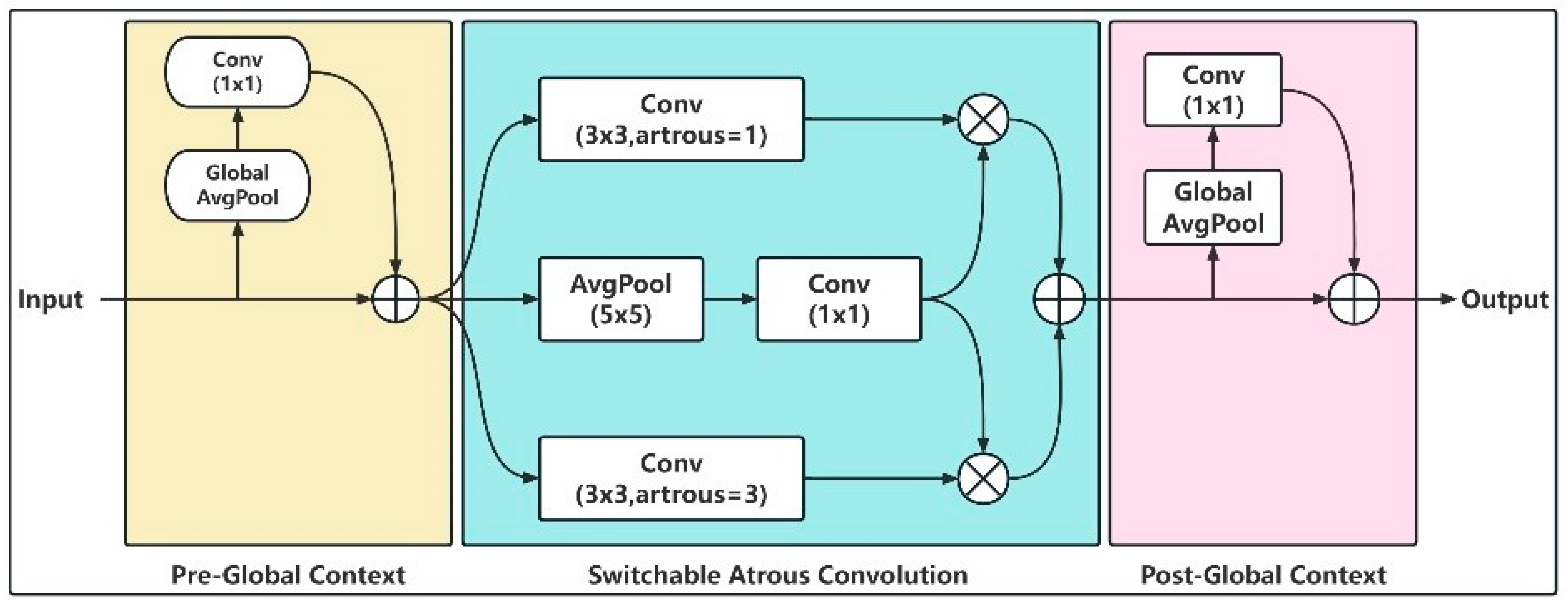
To address the issue of low recognition accuracy caused by shadow occlusion in spur road disease detection, this study introduces the SAConv module into the feature extraction process. This module integrates the cavity convolution’s multiscale receptive field property with the dynamic switching mechanism. The multiscale receptive field property can expand the receptive field by adapting the convolution kernel expansion rate according to changes in object scale and pose, thereby capturing a broader range of contextual information without increasing the convolution kernel’s size or the network’s depth. It enables the model to capture a broader range of spatial features. It is not limited to the local pixels of the disease. On the other hand, the dynamic switching mechanism enables the network to utilize multiple parallel dilated convolutional layers simultaneously with varying expansion rates. It dynamically fuses the results using the Switch Function (SF) to enhance the perceptual range and resolution of the feature map. As shown in Figure 3, its structure consists of three parts: the SAC module (Switchable Atrons Convolution) and two global context modules (Pre-Global Context) [19], attached before and after the SAC module. As the core part, its SCA involves a weighted combination of two convolutional operations with different dilation rates. SAC consists of a switchable dilated convolution and a Switch Function, which first observes the input features with varying dilation rates and then selects the fusion to generate the final output features. The operations share the same weight, reducing the computational effort of the model. The two lightweight global context modules extract image-level semantic information through global average pooling, enhancing the Switch Function’s stability and the sensing field’s global sensing ability. The proposed architecture is conceptually similar to the Squeeze Excitation Network (SENet) [20]. However, SAConv relies entirely on convolutional layers and omits the linear transformations in SENet.

SAConv enhances traditional convolution to improve feature extraction performance through the synergy of multiple components. The global context module extracts image-level semantic information using global average pooling and 1 × 1 convolution, fusing with the input features to enhance the initial perception. The SAC module consists of three branches: two 3 × 3 convolutions with dilation rates of 1 and 3, a 5 × 5 average pooling layer, and a 1 × 1 convolution. Adaptively adjusting the convolution kernel expansion rate expands the sensory field without increasing network depth, allowing for the effective capture of subtle disease features in shadow-obscured regions. Two learnable parameters, γ and β, are introduced in the weighted combination link of different dilation rates’ convolution operations, and when fusing the outputs of two 3 × 3 convolutions with dilation rates of 1 and 3, the weight share of the convolution results with different dilation rates is dynamically adjusted by γ and β to balance the contribution of multiscale features [21] adaptively. The SAConv expression formula is as follows:

$$y=Conv\left( x,w,1\right)\times S\left(x\right)+Conv\left( x,w+\Delta w,r\right)\times \left(1-S\left(x\right)\right)$$

(1)

As shown in Equation (2), x denotes the input feature map, and y represents the output of the convolutional operation. Conv(x,w,r) corresponds to the convolution operation with weight w, r is the hyperparameter, Δw is the trainable weights, and S(x) is the switching function, which can be adaptively adjusted to handle different objects [22]. The weights are dynamically assigned by the trainable parameter Δw and the switching function to enhance the edge feature response to low-contrast lesions, thereby addressing the problem of weak feature loss caused by the traditional ReLU activation function.

SAConv integrates multiscale sensory field characteristics with a dynamic switching mechanism to overcome the challenge of learning small target feature information in traditional convolution, thereby improving the efficiency of feature extraction. SAC module operations share the exact weights, improving the model’s efficiency. Overall, SAConv demonstrates superior adaptability and learning capabilities in addressing the small target detection task, thereby enhancing the network’s effectiveness in handling occlusion and multiscale disease features.

2.2. Building the C2PSA_CAA Module

The latest research results: YOLOv11 by Khanam et al. [17] is an advanced object detection framework that integrates the C2PSA module and spatial attention mechanism; this innovation utilizes the self-attention mechanism to capture long-range dependencies and adaptively weights the features of the target region through a two-branch attention pathway, which significantly enhances the spatial focusing ability of the feature map. The C2PSA module primarily relies on the self-attention block mechanism, specifically the Position-Sensitive Attention Block (PSABlock). However, its capture of local spatial relationships between features is more limited [17]. When dealing with branch-line road diseases susceptible to interference from neighboring targets, especially when there are multiscale diseases in the detection area, C2PSA cannot adequately adapt to the diversity of disease types and the complexity of the background interference. The computational complexity is high, which may affect the efficiency of branch-line road disease detection.

The Context Anchor Attention (CAA) mechanism, as illustrated in Figure 4, is introduced to incorporate long-range contextual information and address the challenges posed by the concurrent occurrence of branch road diseases. CAA module is an efficient spatial attention mechanism designed to enhance the model’s contextual awareness and spatial localization of road disease features [23]. The mechanism is a crucial component in the Progressive Kernel Interaction Network (PKINet), which utilizes average pooling and convolutional operations to capture long-range contextual information and enhance features in the central region [24].

$$F_{l-1,n}^{\mathrm{pool}}=Con{v}_{1\times 1}({\rho }_{avg}(X_{l-1,n}^{(2)}))$$

(2)

As shown in Equation (2), applying a global average pooling operation ${\rho }_{avg}$ to the input features $X_{l-1,n}^{(2)}$ compresses the spatial dimension, allowing for the extraction of global semantic information. This is followed by a 1 × 1 convolution to generate the preliminary features $F_{l-1,n}^{\mathrm{pool}}$. Depth-Separable Stripe Convolution [25] (DWConv) features transformation $F_{l-1,n}^{\mathrm{pool}}$ in the horizontal (1 × k_b) and vertical (k_b × 1) directions, respectively, obtaining $F_{l-1,n}^{\mathrm{w}}$ and $F_{l-1,n}^{\mathrm{h}}$, as shown in Equation (3). The two depth-separable strip convolutions function similarly to a large kernel depth convolution by setting the kernel size k_b = 11 + 2 × l and dynamically expanding the sensory field with the increase in the depth of the network to enhance the long-distance context modeling capability while maintaining computational efficiency [23]. The directional features are convolved 1 × 1 and a Sigmoid activation functions to generate an attention map $A_{l-1,n}$, as shown in Equation (4), which adaptively recalibrates the feature contributions regarding channels [26].

$$\left\{\begin{array}{c}{F}_{l-1,n}^{\mathrm{w}}=DWCon{v}_{1\times k_b}(F_{l-1,n}^{pool})\\ F_{l-1,n}^{\mathrm{h}}=DWCon{v}_{k_b\times 1}(F_{l-1,n}^{\mathrm{w}})\end{array}\right.$$

(3)

$$A_{l-1,n}=Sigmioid(Con{v}_{1\times 1}(F_{l-1,n}^{\mathrm{h}}))$$

(4)

The module effectively enhances the model’s ability to detect targets in complex backgrounds without significantly increasing the computational complexity through lightweight strip convolution (parameter reduction by k_b/2) with dynamic kernel size design.

The CAA module dynamically generates direction-sensitive attention weights through global average pooling with depth-separable bar convolution, effectively capturing the target’s heading features and enhancing features through Sigmoid activation. Combining CAA with the Cross Stage Partial with Parallel Spatial Attention (C2PSA) module and constructing the C2PSA_CAA module at the end of the backbone network can play to the advantage of CAA spatial feature extraction while maintaining the multi-level feature fusion capability of C2PSA. The structure is illustrated in Figure 5. This fusion design enhances the extraction of local spatial details while preserving the C2PSA multiscale feature integration capability, thereby improving the model’s recognition accuracy in multiscale disease scenarios.

2.3. Constructing MCS Hybrid Attention Mechanism

In the feeder road disease detection task, the SAConv module effectively expands the receptive field of the convolutional kernel by dynamically switching the dilation rate (e.g., r = 1 and r = 3), thereby enhancing the multiscale feature extraction capability. A significant expansion rate (r = 5) may over-smooth the edge details when detecting delicate lesions. In contrast, a small expansion rate (r = 1) overlooks the global structure. The attention weights of different regions are assigned by adjusting the field of view of the convolutional kernel. However, this approach makes it difficult to determine which features are more critical to the detection results when facing lesions with significant size differences. This may lead to the missed detection of small targets or feature confusion. Moreover, C2PSA_CAA strengthens the perception of the global context by strip convolution. However, its attentional weight mainly relies on the global average pooling, and its ability to suppress local noise needs to be improved.

To further solve the problems of minor target omission and limited expression of weak features occurring when detecting disease concurrency in feeder roads, this paper constructs the MCSAttention mechanism in the feature fusion and inference stage, mixing multiscale convolution to build the spatial attention, extracting the horizontal, vertical, and global features, respectively, and realizing multi-directional detail retention, with the structure as shown in Figure 6. Its two fully connected layers process the input feature maps by channel attention and derive the weight coefficients of each channel. Moreover, the Sigmoid activation function is applied to generate the interval’s weight values (0,1). It was found that weighting the channel features reduced the effect of redundant information while emphasizing the more critical features related to the disease.

By employing 1 × 3 and 3 × 1 convolution, spatial attention extracts horizontal and vertical spatial information, respectively, and combines it with dilation convolution to enhance the sensitivity of the target at different scale features. Meanwhile, spatial attention utilizes 1 × 5 and 5 × 1 convolutions to adapt to spatial features at different scales. It considers local and global information to generate multiscale feature maps [27]. MCSAttention employs a two-branch pyramid structure to address feature interactions in both the channel and spatial dimensions. In the channel dimension, channel weights are generated by global average pooling (GAP) and maximum pooling (GMP) to suppress disease-independent low-response channels [28,29]. Finally, the inter-channel dependencies are learned through a fully connected layer (FC). Specifically, the input feature map $X\in {\mathrm{R}}^{C\times H\times W}$ (C is the number of channels, and H and W are the height and width) [30] is firstly subjected to global average pooling and global maximum pooling to extract the global information of the channel dimensions, respectively, as shown in Equation (5).

$$\left\{\begin{array}{l}{F}_{avg}^c ={\displaystyle \frac{1}{H\times W}} {\displaystyle \sum _{h=1}^H{\displaystyle \sum _{\omega =1}^W F_{c,h,w}}}\hfill \\ F_{\max }^c ={\max }_{h=1,\cdots ,H;w=1,\cdots ,W} F_{c,h,w}\hfill \end{array}\right.$$

(5)

For global average pooling $F_{\mathrm{avg}}^c$, the pooling results are entered separately by the weighting matrix $W_0\in R^{{\displaystyle \frac{\mathrm{C}}{\mathrm{r}}}\times c}$, bias, $b_0\in R^{{\displaystyle \frac{\mathrm{C}}{r}}}$, $b_0\in R^{{\displaystyle \frac{\mathrm{C}}{r}}}$, and the composition of the multilayer perceptron (MLP) [31,32]. The result after the first fully connected layer [33] is $F{C}_{avg1} =W_0 F_{avgc} +b_0$. After the ReLU activation function [34], we can obtain $\mathrm{ReLU}(F{C}_{avg1})=\max (0,F{C}_{avg1})$. Finally, after passing through the second fully connected layer, we can obtain $F{C}_{avg2} =W_1 ReLU(F{C}_{avg1 })+b_1$. This is the same for global maximum pooling $F_{\max }^c$, as shown in Equation (6).

$$\left\{\begin{array}{l}F{C}_{\max 1}=W_0{F}_{\max }^c+b_0\hfill \\ \mathrm{Re}LU(F{C}_{\max 1})=\max (0,F{C}_{\max 1})\hfill \\ F{C}_{\max 2}=W_{1}ReLU\left(F{C}_{\max 1}\right)+b_1\hfill \end{array}\right.$$

(6)

The final channel attention formula is obtained as shown in Equation (7), where $\sigma$ denotes the Sigmoid activation function [35], c represents the number of neurons, and W₀ and W₁ denote the weight matrices in the multilayer perceptron (MLP) [36].

$$M_c (F)=\sigma (W_1 ReLU(W_0 F_{avgc} +b_0)+b_{1 }+W_1 ReLU(W_0 F_{maxc} +b_0)+b_1)$$

(7)

Similar to the approach in channel attention, two pooling methods are applied to generate feature maps along the channel dimension, as shown in Equation (8).

$$\begin{array}{l} \\ \left\{\begin{array}{l}{F}_{avg}^s ={\displaystyle \frac{1}{C}} {\displaystyle \sum _{C=1}^C{F}_{c,h,w}}\hfill \\ F_{max}^s =ma{x}_{c=1,\cdots ,C} F_{c,h,w}\hfill \end{array}\right. \end{array}$$

(8)

Given that the formula for spatial attention is Equation (9), Norm₁ and Norm₂ is a normalization operation and $f_{conv}$ is a convolution operation [37]. This mechanism focuses the spatial location of the disease and suppresses the background noise interference.

$$M_s (F)=\sigma (Nor{m}_2 (Nor{m}_1 (f_{conv} (f_{3\times 1(v)} (f_{1\times 3(h)} ([F_{avg}^s ;F_{max}^s]))+f_{5\times 1} (f_{1\times 5} ([F_{avg}^s ;F_{max}^s]))))))$$

(9)

As shown in Equation (10), the final augmented feature map, Y, is obtained in the following manner. In Equation (10), ⊙ denotes elemental multiplication and ⊗ denotes channel multiplication or spatial multiplication, depending on the broadcast mechanism and dimension of the attention graph [38].

$$Y=X\odot (M_c (F) \otimes M_s (F))$$

(10)

The k_size = 3 and k_size = 17 reflect the equivalent receptive field design of the multiscale convolutional kernel rather than directly corresponding to the physical size of a single convolutional kernel. k_size = 3 refers to an equivalent receptive field of 3 × 3, which is actually achieved by combining 1 × 3 and 3 × 1 strip convolutions. A 1 × 3 convolution is responsible for the horizontal operation and focuses on extracting the horizontal disease features. A 3 × 1 convolution is responsible for vertical operation, capturing vertical disease features. While traditional 3 × 3 convolution introduces redundant edge information, the strip convolution kernel reduces noise interference by constraining the direction of convolution while reducing the number of parameters [39]. k_size = 17 represents the equivalent sensory field extension achieved by stacking multiple levels of strip convolution kernels (5 × 1 and 1 × 5) instead of a single convolution of 17 × 1 or 1 × 17 for capturing the long-range context of the disease and background relationship. Moreover, 17 is an odd size, facilitating symmetric filling and avoiding feature map bias [40]. A 1 × 5 bar convolution associates the diseased area with its surrounding environment, and a 5 × 1 convolution models semantic associations between longitudinal targets and neighboring areas. Combining the two subsequent operations approximates the global coverage capability of 17 × 1 with fewer parameters. Spur road diseases are often intertwined with complex backgrounds, and traditional small-kernel convolution is prone to fall into localized noise. With multilevel strip convolution stacking, the model captures the long-range dependencies of the disease about the background. A 17 × 1 convolution may introduce noise in irrelevant directions.

In contrast, 5 × 1 with 1 × 5 convolution fits the geometric properties of the target better by constraining the perceived directions. Traditional 3 × 3 convolution introduces redundant oblique information interference. In contrast, 3 × 1- and 1 × 3-oriented bar convolution reduces noise interference by constraining the direction of convolution while lowering the computation. k_size = 3 bar convolution kernels capture the extension characteristics of the cracks, respectively, to strengthen the model’s ability to perceive the geometrical shape of the disease. Focusing on the spatial relationship between local pixels helps avoid blurring details caused by large kernel convolutions. k_size = 17 convolution complements k_size = 3 convolution, with the former focusing on fine-grained local features and the latter integrating global semantic information, thereby realizing adaptive balancing of multiscale features through feature map weighted fusion (e.g., Sigmoid activation) [41]. In summary, MCSAttention optimizes multilevel features through channel and spatial attention synergy with multiscale convolutional adaptive weighting. The mechanism utilizes 1 × 3 and 3 × 1 convolutions to extract target heading features directionally, combined with 5 × 1 and 1 × 5 convolutions to capture global semantic information. It reduces the false detection rate by suppressing irrelevant backgrounds through channel and spatial attention, dynamically augmenting the weights of diseased regions.

2.4. Optimization of the Loss Function

While YOLOv11’s bounding box regression loss conventionally employs Complete Intersection over Union (CIoU) [42], this approach exhibits limitations in pavement distress detection due to heterogeneous target significance across spatial regions, morphological diversity of defects (e.g., cracks, potholes), and complex background interference. CIoU prioritizes geometric shape matching by penalizing centroid misalignment and aspect ratio discrepancies. However, pixel-wise weight distribution and regional class imbalance are neglected by CIoU, which particularly degrades the detection accuracy of edge-localized defects. Furthermore, penalties for low-quality training samples (e.g., inaccurately annotated bounding boxes) are amplified by CIoU’s reliance on geometric metrics, and the risk of overfitting is increased when handling imperfect datasets [43]. This issue is particularly exacerbated in feeder road applications, where labeled datasets are scarce and often contain human-induced annotation inaccuracies resulting from manual data collection. CIoU is replaced with Weighted Intersection over Union version 3 (WIoU v3) to address these challenges as this study’s bounding box regression loss. Dynamic weighting based on target complexity and annotation quality is introduced by WIoU v3, adaptively balancing penalties for high-quality and low-quality samples. By incorporating spatial importance maps and annotation confidence scores, the adverse effects of label noise are mitigated by WIoU v3. At the same time, the focus on critical regions (e.g., crack edges, partially obscured potholes) is enhanced, thereby improving robustness and detection precision in real-world pavement maintenance scenarios. The traditional IoU-based loss is enhanced in WIoU v3 through the incorporation of a dynamic weighting tensor [44], where pixel-wise contributions are adaptively modulated according to spatial coordinates or target significance, enabling critical regions (e.g., crack nuclei and repair zones) to be systematically prioritized. This mechanism mitigated detection imbalances by adaptively refining bounding box regression for diverse pathologies while improving sensitivity to small-scale defects.

$$\left\{\begin{array}{l}r={\displaystyle \frac{\beta }{\delta {\alpha }^{\beta -\delta }}}\hfill \\ \beta ={\displaystyle \frac{{L^{*}}_{IoU}}{L_{IoU}}}\in [0,+\infty )\hfill \end{array}\right.$$

(11)

As shown in Equation (11), r is a key parameter in the dynamic nonmonotonic focusing mechanism (FM), which is used to adjust the gradient contribution of different quality anchor frames, and it is calculated from the anomaly β of the anchor frames. δ and α are hyperparameters, and when β = δ, r = 1; when β deviates from δ, r is dynamically adjusted so that the medium-quality anchor frames obtain higher gradient gain, while the gradient gain of the high-quality and low-quality anchor frames is suppressed, thus enhancing the model’s focus on ordinary quality samples.

The final loss function integrates a normalized Wasserstein distance, computed via exponential terms. It is presented in Equations (12) and (13), where W_g and H_g denote the width and height of the minimal enclosing bounding box, (x,y) and (x_gt,y_gt) represent the predicted and ground-truth bounding box centroids, respectively [45]. To prevent R_WIoU from hindering convergence gradients, W_g and H_g are separated from the computational graphs to eliminate impediments to convergence effectively, and no new metrics have been introduced, such as aspect ratio [2].

$$R_{\mathrm{WIoU} \mathrm{v}3}=\exp [{\displaystyle \frac{{(x-x_{gt})}^2+{(y-y_{gt})}^2}{({W_{\mathrm{g}}}^2+{H_{\mathrm{g}}}^2)}}]$$

(12)

$$L_{\mathrm{WIoU} \mathrm{v}3}=r\times R_{\mathrm{WIoU}}\left(1-\mathrm{IoU}\right)$$

(13)

3. Test Results and Analysis

3.1. Dataset Preparation

3.1.1. Processing and Analysis of Datasets

At this stage, open-source road disease datasets (e.g., RDD, UAV-PDD2023 (https://www.kaggle.com/c/uav-pdd2023 (accessed on 25 April 2025))) primarily focus on urban road images, whereas dataset images for feeder road diseases are scarce. Therefore, feeder road disease images are collected by field shooting and open dataset screening, for each acquired image contains at least one disease type. The road disease data collection include manually taking pictures of feeder roads around Wanbailin District, Taiyuan City, and selecting sample pictures of feeder road diseases from the open dataset RDD-2022 (published by the University of Tokyo) [46]. The data organization and calibration methodology draw on the framework proposed in the literature [47] to ensure annotation quality and consistency in spatial alignment. Disease categories are categorized according to the Technical Condition Assessment Standard (JTG5210-2018) [48], and annotations are generated using Labelimg to delineate bounding boxes and disease types, as shown in Figure 7. The dataset comprises various scenarios, including light changes, partial shading by vegetation, and multiscale disease coexistence.

To solve the problem of unbalanced distribution of disease categories in the dataset, extremely rare or pathologically unclear annotations are excluded, and five typical disease types commonly found on feeder roads are retained: transverse cracks (D00), longitudinal cracks (D10), reticulation cracks (D20), potholes (D40), and repairs (Repair). The photos of potholes and repair types of diseases are relatively few in the dataset RDD-2022, and the scenarios are relatively homogeneous, which limits their application in real scenarios. To ensure the test’s feasibility and improve the network model’s generalization ability for various diseases across different external environments and light intensities, the Deep Convolutional Generative Adversarial Network (DCGAN) is employed for data enhancement. In addition to expanding the samples using DCGANs, we performed geometric transformations on the raw data (e.g., random rotations and flips to simulate different shooting angles).

After rigorous data organization, the final dataset includes 13,063 high-resolution images of feeder road diseases. To ensure the validity of the experiment, the dataset is divided into a training set (10,449 images), a validation set (1307 images), and a test set (1307 images) by stratified random sampling in a ratio of 8:1:1, and a proportional representation of lesion categories is maintained among the subsets. This hierarchical approach reduces the risk of overfitting while maintaining sufficient sample diversity for a robust evaluation of the model under real-world conditions.

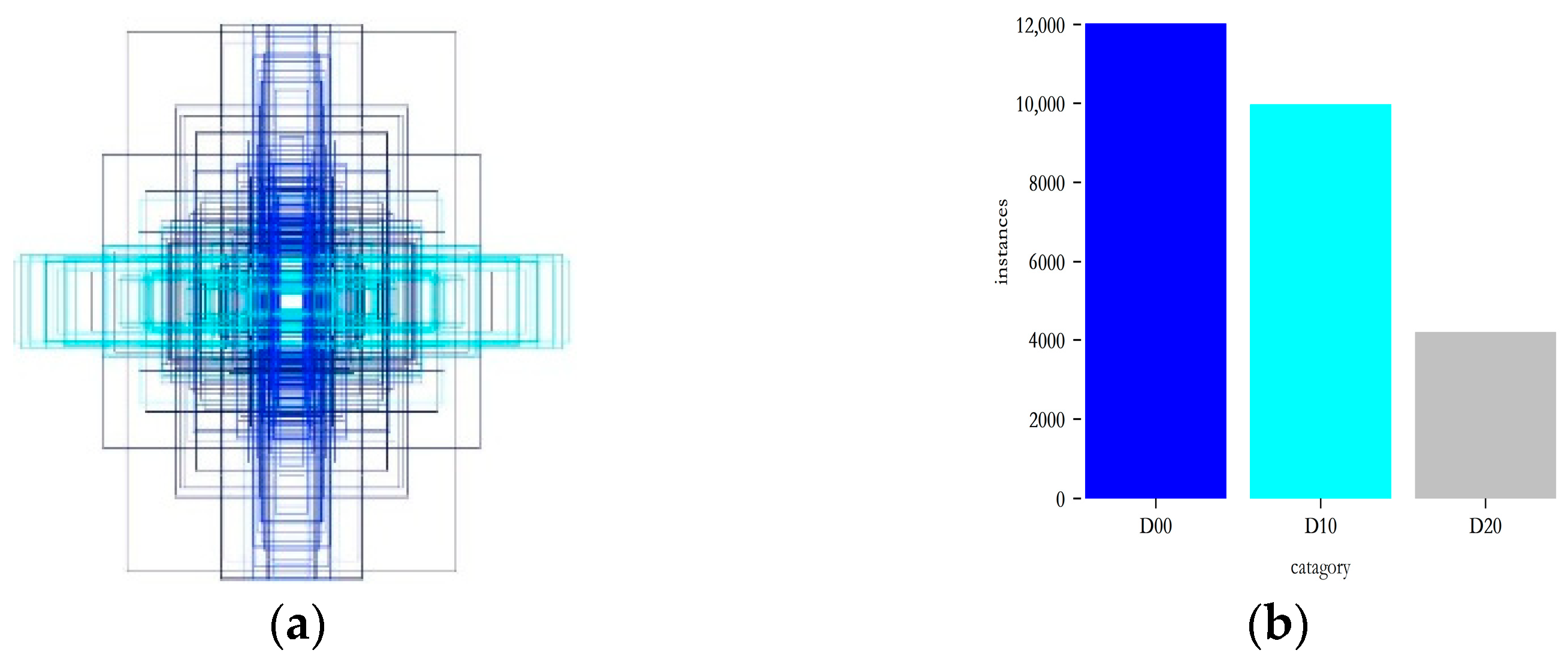
Figure 8 illustrates the size and number of labeling boxes and number of cracks in the dataset, which shows that the size of the labeling boxes varies greatly, and most of them are small-size labeling boxes, indicating that there are more small target samples. The size of the labeling box varies greatly, and most of them are small-sized, indicating that there are more small target samples, which increases the difficulty of detection and identification of the model. The number of samples in each category indicates that the crack category includes samples with transverse cracks, longitudinal cracks, mesh cracks, and other types of cracks. Cracks are the more common feeder road diseases; hence, they are more numerous, and most patching category samples are concentrated on national and provincial highways, resulting in a relatively small number of disease types. Diseases are mainly focused on national and provincial highways. Hence, the number of repair-type diseases is relatively small, but the number of disease-type samples is balanced, which can meet the test demand.

3.1.2. Data Augmentation for Few-Shot Images

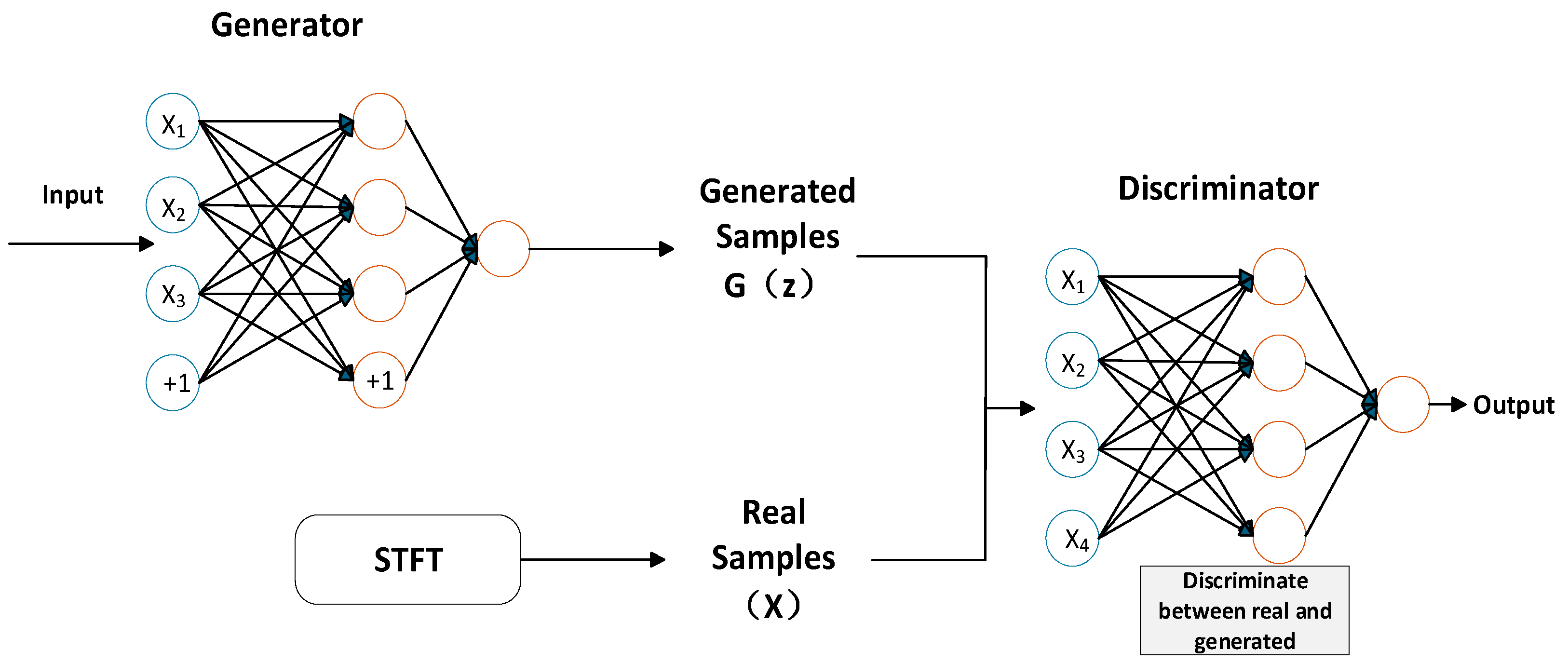
DCGAN is a specialized variant of Generative Adversarial Networks (GANs) designed for image enhancement tasks under limited-sample conditions, such as scenarios involving mesh cracks or patch reconstruction. As depicted in Figure 9, the adversarial framework comprises two neural networks: generator G and discriminator D. Generator G receives input samples from a latent noise distribution and synthesizes enhanced images, while discriminator D is trained to distinguish between actual samples (derived from Short-Time Fourier Transform (STFT)-processed data X) and generated outputs from G [49]. During training, G aims to approximate the real data distribution by minimizing the divergence between the synthesized and authentic samples, whereas D optimizes its ability to classify the source of inputs. This adversarial process is formalized as a minimax optimization problem:

$$\min \max V(D,G)=E_{x~P_{data}}(x)[\log D(x)]+E_{z~P_{G(z)}}[\log (1-D(G(z))]$$

(14)

As shown in Equation (14), p_data denotes the real data distribution, p_z represents the latent noise distribution, x follows the real distribution, and z is drawn from the simulated G, as assumed in $x~P_{\mathrm{data}}(x)$, $z~P_{G\left(\mathrm{z}\right)}$ [50]. The iterative training continues until D achieves an equilibrium state where it can no longer reliably differentiate between actual and generated samples, indicating convergence of the model.

Therefore, to enhance model generalization, a Generative Adversarial Network performs data augmentation and generalization of the two sample-less diseases, mesh crack and repair. The original sample images of the two diseases, mesh crack and repair, are shown in Figure 10, and the images of mesh crack and repair diseases generated by DCGAN are shown in Figure 10, where the first row is the mesh crack and the second row is the repair disease.

3.2. Test Environment

A standardized experimental environment was established to ensure the reproducibility and validity of all experiments. The configuration is as follows:

Hardware: Intel Core i9-10900 CPU (Intel Corporation, Santa Clara, CA, USA), NVIDIA Quadro RTX 5000 GPU (1638MiB; NVIDIA Corporation, Santa Clara, CA, USA);

Software: Windows 10, PyTorch 2.0.1 framework, Python 3.9.20, CUDA 11.7 toolkit;

Training Protocol: 300 epochs, batch size of 16, Stochastic Gradient Descent (SGD) optimizer with momentum (0.937), initial learning rate of 0.01 (Cosine decay schedule), and weight decay (L2 regularization).

All hyperparameters (e.g., anchor box ratios, non-maximum suppression thresholds) remain at default configurations to isolate the impact of architectural innovations. This setup ensures consistent computational resource allocation and minimized variability across trials, and alignment with best practices for deep learning benchmarking in computer vision applications is achieved.

3.3. Evaluation of Indicators

To comprehensively evaluate the model’s performance, precision (P) and recall (R) are adopted as primary evaluation metrics, complemented by mean average precision (mAP@0.5:0.95) and F1-score to quantify accuracy improvements and class-specific detection robustness. Computational efficiency is assessed via Giga Floating Point Operations per Second (GFLOPs) and total trainable parameters (Params), where lower values indicate reductions in computational overhead and memory footprint, respectively. F1-score, the harmonic mean of precision and recall, provides a balanced measure of model efficacy under class imbalance. Meanwhile, mAP@0.5:0.95 evaluates detection accuracy across multiple Intersection over Union (IoU) thresholds (0.5 to 0.95 in 0.05 increments), reflecting robustness to localization errors. This multi-faceted evaluation framework ensures rigorous detection performance and deployment feasibility assessment in resource-constrained environments.

3.4. Analysis of Experiments

3.4.1. Tests on the Effectiveness of the MCSAttention Mechanism

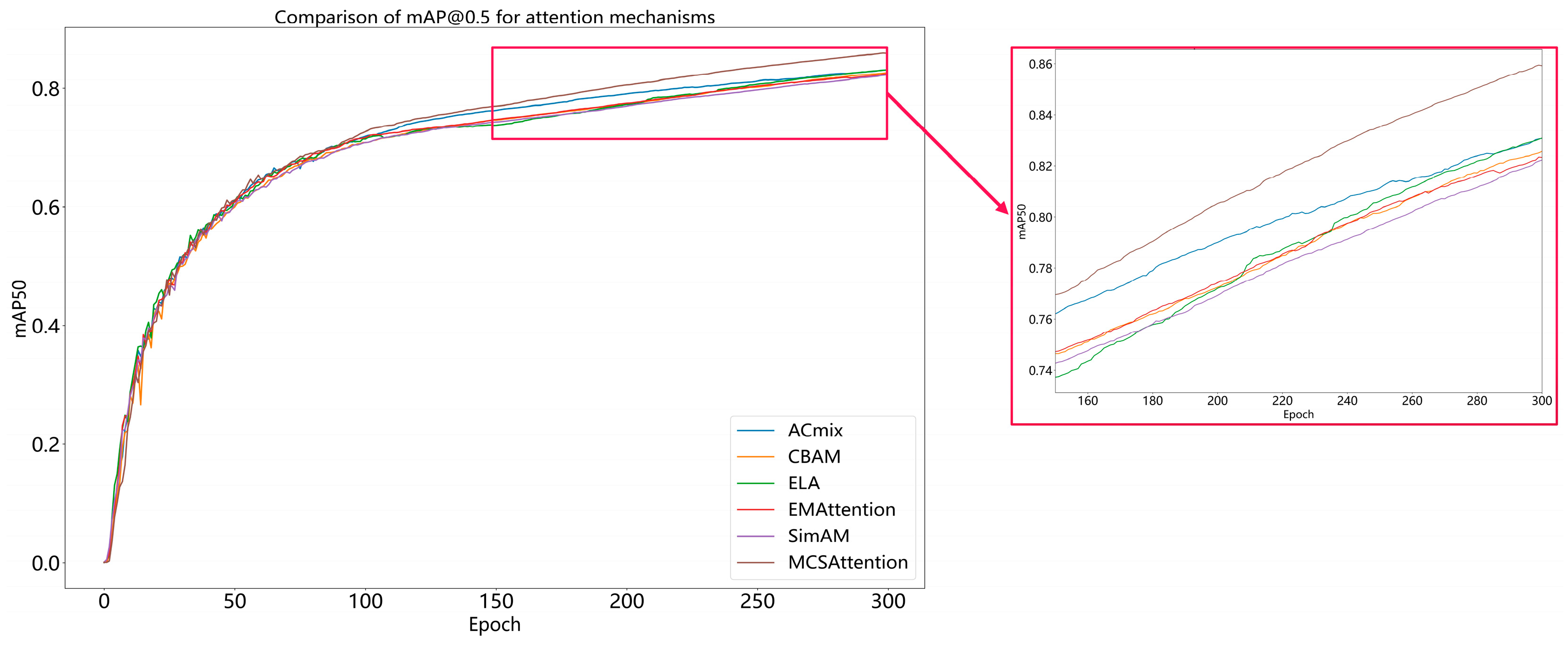
To evaluate the efficacy of the self-constructed MCSAttention module for detecting multiscale disease scenarios on feeder roads, comparative experiments are conducted against common attention mechanisms with comparable parameter counts and computational budgets, as summarized in

Table 1. Performance comparison of different attention modules.

Model Name	P/%	R/%	mAP50/%	Params/106	GFLOPs
YOLOv11	87.4	74.0	81.6	2.7	6.3
+CBAM	87.4	76.4	82.6	2.7	6.4
+ELA	87.8	75.2	83.1	2.7	6.5
+ACmix	87.8	73.6	83.1	2.9	7.0
+EMAttention	88.1	73.8	82.3	2.6	6.4
+SimAM	88.6	72.6	82.2	2.6	6.3
+MCSAttention	89.1	76.8	85.9	2.6	6.5

. MCSAttention demonstrates superior detection accuracy, achieving a 4.3% improvement in mAP@50 and a 2.8% gain in recall (R) compared with baseline models. Although SimAM exhibits the lowest computational overhead (1.2 GFLOPs), marginal performance gains (0.6% mAP@50 improvement) are yielded by it, and its limited adaptability to complex multiscale scenarios is highlighted. By contrast, a hierarchical architecture is possessed by MCSAttention. Multiscale convolutional kernels and spatial-contextual attention are integrated by it (MCSAttention), which enables robust feature discrimination across varying defect scales without significantly increasing the computational complexity (ΔGFLOPs < 0.3). These results validate the capability of MCSAttention to balance accuracy and efficiency.

A comparative analysis of recall–performance curves between the proposed MCSAttention module and existing attention mechanisms is presented in Figure 11, demonstrating the superior robustness of MCSAttention in detecting multiscale and occluded road distresses. This enhancement is attributed to the hierarchical architecture of MCSAttention. This architecture uses multiscale convolutional kernels and adaptive spatial-contextual weighting to prioritize fine-grained defect features while background interference is suppressed. The results validate the capability of MCSAttention to maintain high sensitivity across diverse disease scales and occlusion scenarios, which is a critical requirement for reliable automated inspection of feeder road infrastructure.

3.4.2. SAConv Module Effectiveness Tests

The receiver field is dynamically adjusted by SAConv in response to variations in object scale and pose, and adaptive feature extraction across diverse spatial contexts is enabled. As demonstrated in

Table 2. Performance comparison of different convolutional modules.

Model Name	P/%	R/%	mAP50/%	Params/106	GFLOPs
YOLOv11	87.4	74.0	81.6	2.7	6.3
+DSConv	86.0	74.9	83.0	2.6	4.8
+DWConv	87.0	76.1	83.5	2.1	4.9
+SPDConv	84.3	69.2	78.5	2.3	5.5
+GhostConv	85.9	74.1	82.5	2.3	5.6
+DBB	87.5	74.8	82.9	3.2	8.9
+SAConv	86.7	77.2	84.1	3.1	4.8

, when five convolutional methods used for enhancing disease feature extraction [20] are compared to verify the efficiency of the convolution proposed in this paper, it is possible to find that SAConv outperforms five established convolutional variants in disease feature extraction efficiency. After comprehensive analysis and comparison, the addition of SAConv sacrifices model precision and light weight to a lesser extent while obtaining improvements in other comprehensive indexes. The comparison reveals that the model recall and computational complexity are most significantly improved with the addition of SAConv, reaching 77.2% and 4.8, respectively. The model with the addition of SAConv also has the highest mAP₅₀ among the models compared, especially in road disease detection, where mAP₅₀ has an irreplaceable core value [21]. Dilated convolution principles are integrated by this hybrid convolution to systematically expand the receptive field through hierarchical dilation rates, and thereby, this hybrid convolution bridges spatial discontinuities in a structured manner. Long-range local features are captured while the addition of SAConv mitigates background interference (e.g., soil or vegetation occlusions), and the ability of the model to discern subtle pathologies under cluttered conditions is enhanced. In addition, SAConv improves the accuracy of disease detection by reducing the number of parameters in the model with an optimized weight calculation. SAConv has two dual advantages: enhanced spatial awareness and computational frugality.

3.4.3. Ablation Experiment

To validate the efficacy of the proposed architectural enhancements, an ablation experiment is conducted using YOLOv11 as the initial model. The results are summarized in

Table 3. Results of ablation experiment.

Initial Model.	WIoU	SAConv	C2PSA_CAA	MCSAttention	P/%	R/%	mAP50/%	Params/106	GFLOPs
√	×	×	×	×	87.4	74.0	81.6	2.6	6.3
√	√	×	×	×	88.2	74.7	83.4	2.6	6.3
√	×	√	×	×	86.7	77.2	84.1	3.2	4.8
√	×	×	√	×	88.4	76.9	84.0	2.6	6.3
√	×	×	×	√	89.1	76.8	85.9	2.7	6.5
√	×	√	√	×	87.8	78.0	85.8	3.2	4.8
√	×	√	√	√	88.0	78.1	86.7	2.7	6.5
√	√	√	√	√	89.8	82.4	89.4	3.3	5.0

, and the original YOLOv11 achieves a mAP@50 of 81.6% and a recall of 74.0% on the test set. When the WIoU v3 function is introduced, comparable computational and parametric budgets are maintained, while the mAP@50 improves by 1.8% (to 83.4%), and the precision increases by 0.8% (to 88.2%). This improvement underscores the effectiveness of WIoU v3′s dynamic weighting mechanism. In this mechanism, critical regions are prioritized during bounding box regression. SAConv introduces an adaptive context integration mechanism. This mechanism guides and fuses the contextual information of the input feature maps during the convolutional computation process. GFLOPs are reduced by 20% with the addition of SAConv, while the model parameters increase by only 0.7 M, demonstrating its efficiency in balancing complexity and performance. Concurrently, when adding SAConv, mAP@50 is improved by 2.5%, and recall is improved by 3.2%. When the MCSAttention module is further integrated, mAP@50 is boosted to 85.9% (+4.3%), and recall is boosted to 76.8% (+2.8%), demonstrating its capability to refine feature discriminability across scales. Finally, the model’s ability to recognize features is further enhanced by C2PSA_CAA through synergizing global contextual dependencies and local spatial saliency. Performance is elevated to 84% mAP@50 and 76.9% recall, while the computational overhead of the model remains unchanged. Collectively, the challenges of feeder road disease detection have been positively contributed to and solved by these innovations.

The inherent limitations of SAConv in feature localization accuracy and its propensity for missed detections are addressed by the synergistic integration of the SAConv and C2PSA_CAA modules. The mAP@50 is improved by 4.2% and the recall by 4%, significantly enhancing the model’s sensitivity to subtle disease characteristics. Combined with the multiscale MCSAttention module, this framework leverages synergistic multiscale learning mechanisms to refine feature discriminability. A 5.1% improvement in mAP@50 and a 4.1% increase in recall are achieved compared to the initial model. Notably, when all four proposed modules are fully integrated, the proposed modules collaborate and cooperate; SAConv first generates multiscale features by adaptively adjusting the expansion rate of the convolution kernel, expanding the receptive field to capture local disease features and global semantic relations. Then, C2PSA_CAA processes these features and applies horizontal and vertical strip convolutions to generate directional attention masks, dynamically enhancing critical regions while maintaining the multilevel fusion capability of C2PSA. MCSAttention employs pyramidal cross-scale attention, which combines channel importance (via GAP/GMP) with spatial directionality (1 × 3/3 × 1 for directionality, 1 × 5/5 × 1 for distant context) combined with further optimized and refined features. This combination allows the model to emphasize disease-specific patterns at different scales adaptively. Finally, WIoUv3 incorporates spatial importance maps and annotated confidence scores into the loss function, mitigating the effects of label noise while penalizing critical areas of disease features more severely. This synergy forms a closed loop where SAConv provides the underlying multiscale features, C2PSA_CAA refines the spatial attention, MCSAttention dynamically balances the feature contributions, and WIoUv3 optimizes the training stability. As validated by the ablation study, this synergistic approach increased mAP@50 from 81.6% (Initial model) to 89.4%, indicating a systematic improvement in detection performance through the interaction of complementary modules, as shown in Table 3. The test results show that the proposed model achieves 3.3 M parameters with a computational complexity of 5.0 GFLOPs. This represents a 21% reduction in computational complexity, as quantified by GFLOPs, while maintaining parameter efficiency (ΔParams < 0.8 M), meeting the requirements for lightweight deployment scenarios.

3.4.4. Comparative Experiments

The ablation studies described in the preceding sections validated the efficacy of the proposed framework. To further benchmark its performance for feeder highway disease detection, a comparative analysis is conducted against several mainstream models, including RetinaNet, Faster-RCNN, SSD [51], YOLOv8n, YOLO11n, and the model from Document 11 et al. As summarized in

Table 4. Results of ablation experiments.

Modules	P/%	R/%	mAP50/%	mAP50–95/%	Params/106	GFLOPs	FPS
RetinaNet	63.8	49.8	63.8	38.5	32.06	69.3	14.1
Faster-RCNN	79.7	82.5	66.5	39.0	43.9	101.4	11.2
SSD	28.3	61.2	40.1	22.1	12.9	7.48	41.7
YOLOv3-tiny	88.7	78.4	84.8	58.4	12.1	18.9	294.1
Document 11	78.6	64.1	79.0	52.3	6.01	13.0	122.7
YOLOv6n	79.3	63.9	72.8	48.2	4.23	11.8	312.5
YOLOv7-tiny	86.3	78.6	85.7	52.3	6.03	13.2	238.1
YOLOv8n	87.6	76.0	83.4	56.4	3.01	8.1	322.6
YOLOv9t	80.9	71.9	78.3	53.5	1.97	7.6	256.4
YOLOv10n	84.5	72.3	80.7	55.8	2.70	8.2	312.5
YOLO11n	87.4	74.0	81.6	56.0	2.58	6.3	322.6
Ours	89.8	82.4	89.4	63.8	3.28	5.0	238.1

, when the data in the table are compared, it can be seen that the two-stage model Faster-RCNN compared in this study performs better in terms of detection accuracy but seems to perform poorly in terms of model complexity and arguments. The proposed algorithm achieves 89.8% precision, 82.4% recall, and 89.4% mAP@50. Notably, compared to the efficient YOLOv9t (smallest model size), the parameters are increased by only 1.31 M by the proposed framework, while the computational complexity is reduced by 34.2% (quantified via GFLOPs). The results demonstrate efficiency trade-offs, achieving a 22.9% improvement in mAP@50 over Faster-RCNN and 7.8% over YOLO11n. However, after the YOLOv11 model is added to the SAConv module, the FPS decreases from 322.6 to 256.2. This is mainly because the core component of SAConv, the SAC module, contains multiple branches, which need to weight and combine the results of the convolution of different nulls, introduce the learnable parameters γ and β to adjust the weighting ratio in the process dynamically, and extract image-level semantic information through the global context module. These additional computational steps increase the computational effort of the model, resulting in a decrease in the number of images processed per unit of time, which leads to a decrease in FPS. However, while the SAConv module improves the model’s ability to capture subtle disease features in shaded occlusion regions, it significantly improves the detection accuracy at the expense of a certain speed, which overall helps to improve the network’s processing of occluded, multiscale disease features.

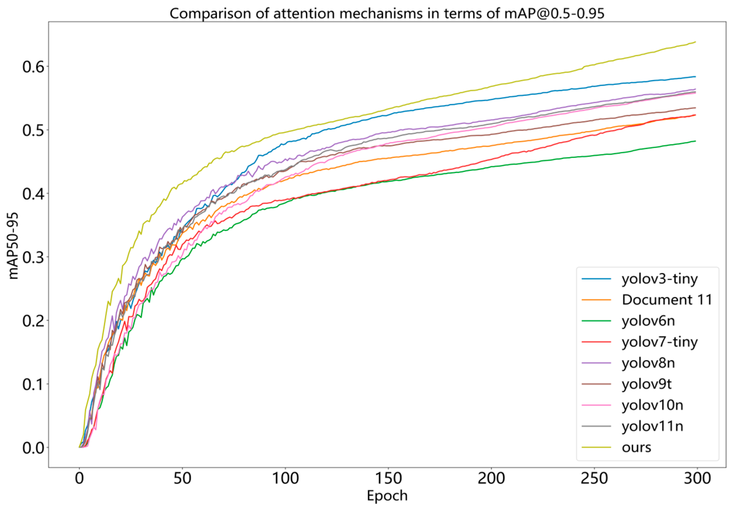
Because the two-stage inspection model possesses high computational complexity and the real-time requirements of feeder roads are not met, the single-stage inspection model described above is used for comparison. The mAP_50–95 metrics curve of the YOLOv11 algorithm compared to the algorithm presented in this paper is illustrated in Figure 12. Figure 12 shows that our model has the fastest rise in mAP_50–90 at the beginning of training. Compared to the other models, after about 40 epochs, our model curve shows a more significant rise, and it eventually maintains a higher mAP_50–90 value. On the whole, our model has higher detection accuracy and a better optimization effect.

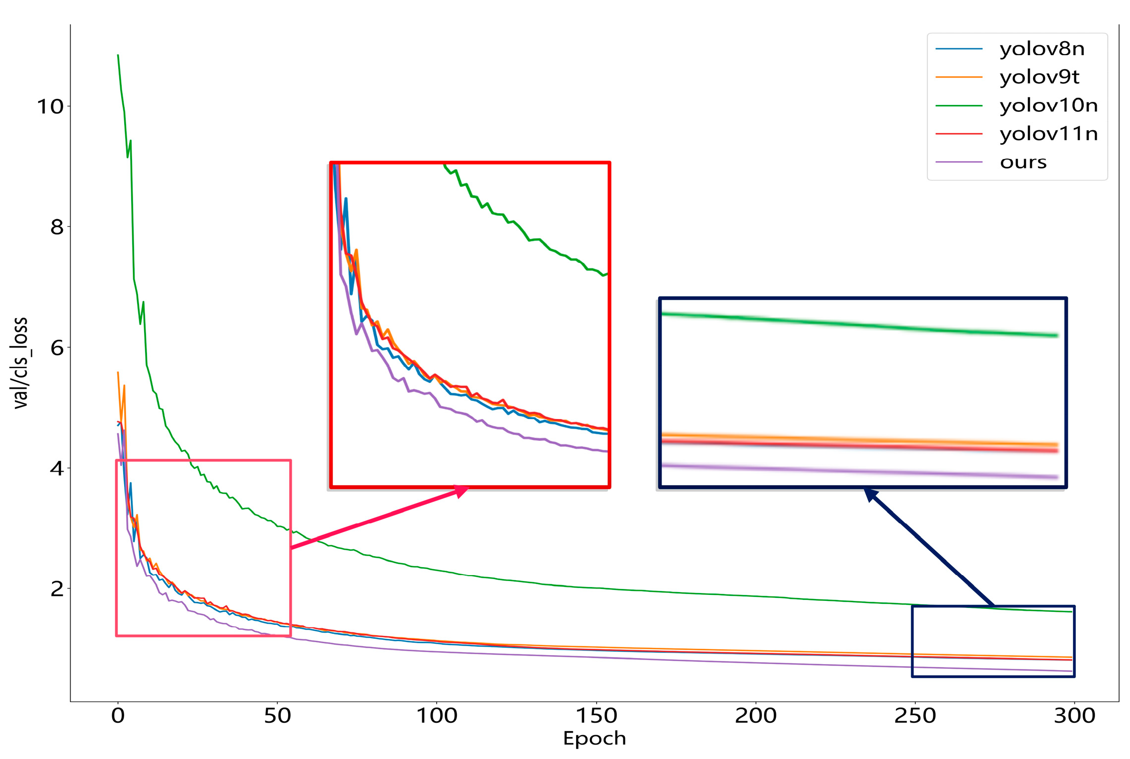
As can be seen from Table 4, the update speed of the recent YOLO models is relatively fast. For models such as YOLOv3 and YOLOv7, although their performance in terms of accuracy is not bad, in terms of model complexity and parametric quantitative indicators, it does not meet the real-time requirements of feeder road disease detection. Figure 13 shows that at the beginning of training, our model shows a slight decrease in the loss value. Also, at the beginning, the loss value is low, and after about 30 epochs, it stabilizes, and eventually, a low loss value is maintained by it. This indicates that in terms of both learning efficiency and generalization ability, our model is superior to the YOLOv8n, YOLOv9t, YOLOv10n, and YOLOv11n models, and more stable and lower loss values are exhibited by it.

3.4.5. Evaluation of Practical Application Testing

To address the challenge of detecting diseases in complex feeder road scenarios, we conducted a comparative analysis between the proposed network and YOLOv11, a newer version of the YOLO series. Figure 14 shows the comparison of disease detection in a feeder road scenario with tree shadows, Figure 15 shows the comparison of disease detection in a feeder road scenario with multiple types and scales of concurrent diseases, Figure 16 shows the comparison of disease detection in a feeder road under different geographic conditions, and Figure 17 shows the comparison of disease detection in a feeder road under different weather conditions, in which we have selected representative images and plotted the network’s heat map.

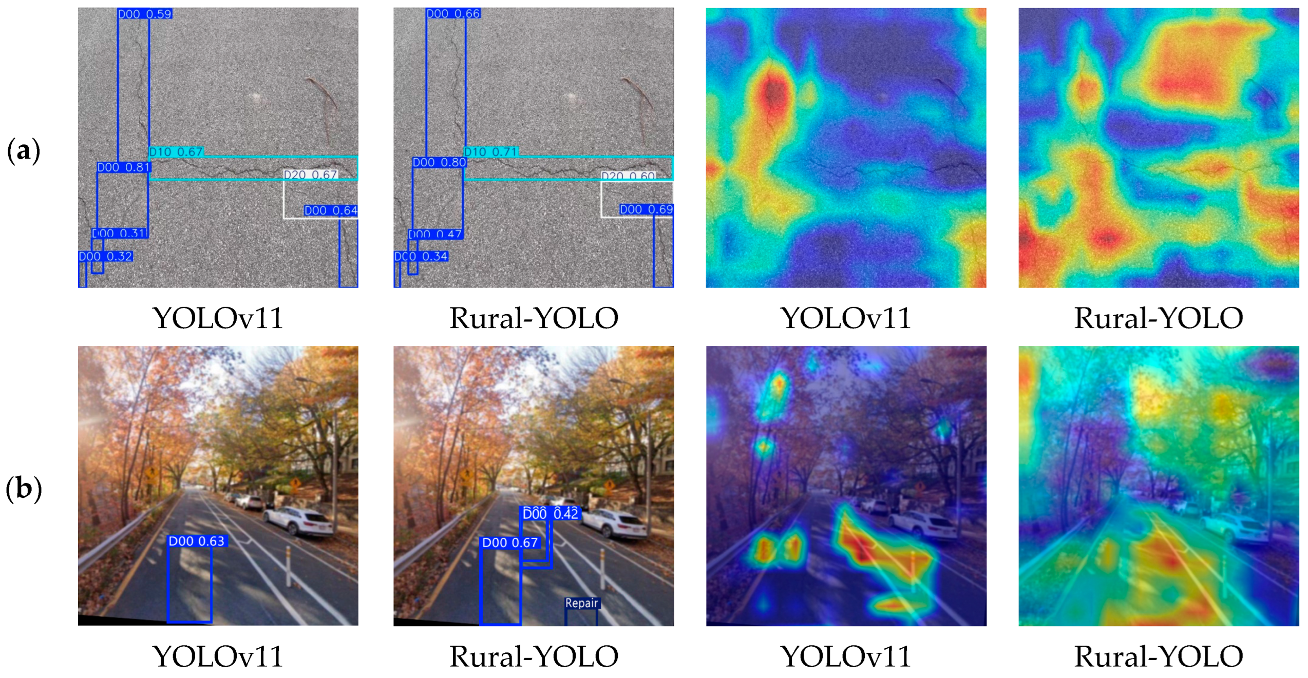
Rural-YOLO’s modules can work synergistically, and SAConv dynamically adjusts the dilation rates, adeptly handles local and global feature relationships, and guides the CAM thermogram to focus on the edge of the disease, providing high-quality bounding-box primaries for WIoUv3. C2PSA_CAA applies spatial attention to suppress shading interferences, focuses on the diseased region, and enhances the thermogram’s response to the direction of the disease through strip convolution response. MCSAttention, on the other hand, enhances feature fusion and contextual correlation to increase the model’s adaptability to different environments. Meanwhile, the synergistic optimization of heat map distribution reduces the background noise interference and lowers the false detection rate. Wiou v3 balances the penalty weights of high-quality and low-quality samples to optimize bounding box regression accuracy. SAConv provides the basis for multiscale feature extraction, and C2PSA_CAA focuses on different disease types. MCSAttention integrates contextual information and combines with WIoUv3 dynamic gradient adjustment to optimize bounding box regression accuracy.

Figure 14 and Figure 15 show that both missed and false detections occurred in the YOLOv11 detection, making it challenging to balance the responses to different sizes and types of disease features. Inter-module coordination enabled Rural-YOLO to generate more comprehensive detection frames and heat maps, thereby improving its detection accuracy. The heat maps generated by Rural-YOLO also evenly covered various disease areas, focusing more on the actual disease area.

As shown in Figure 16 and Figure 17, in the comparison diagrams of disease detection on feeder roads under different geographic and weather conditions, YOLOv11 detects frequent omissions and misjudgments. Its single feature extraction mechanism is challenging to adapt to the drastic changes in features brought about by weather variations and geographic differences, which leads to an imbalance in the model’s response to different scales and types of diseases. Rural-YOLO effectively enhances the robustness of disease features across various weather conditions and complex geographical environments. Its generated detection frames better fit the disease boundaries in scenes with changing conditions. At the same time, the heat maps more evenly cover different areas of the disease, reducing the impact of weather and geographical factors on detection performance. This verifies the model’s ability to generalize to complex real-world scenarios.

3.4.6. Analysis of Generalization Tests

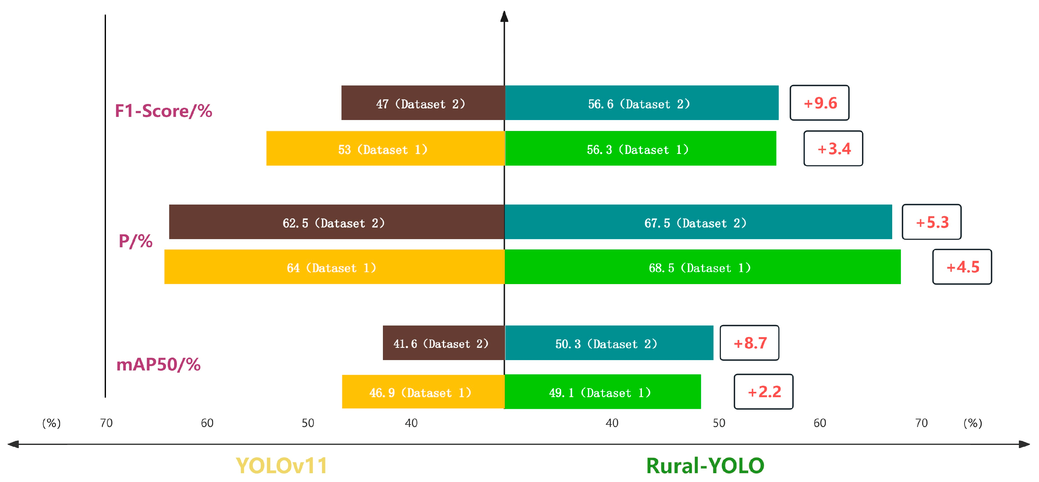
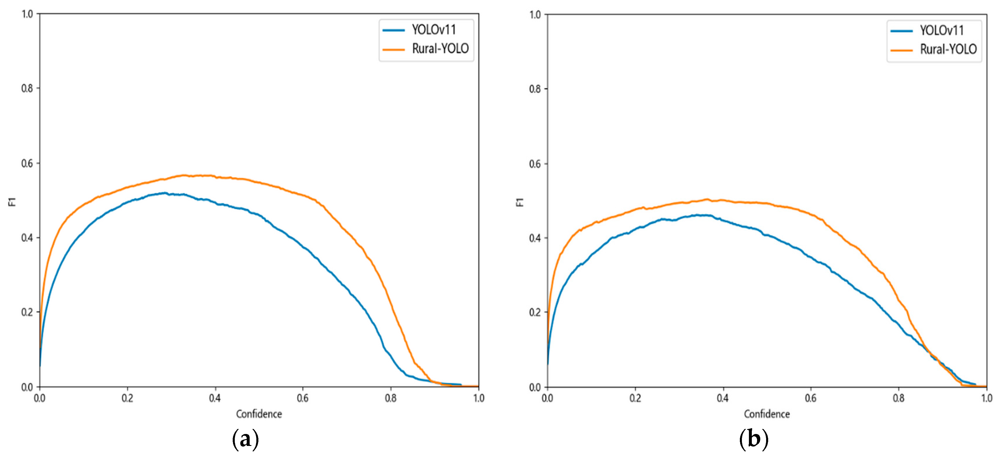
This test selects the same type of city road diseases from the RDD2020 and SODA competition datasets [46]. Some of the same kinds of disease images collected are added as the dataset used for the comparison tests (credited as dataset 1 and dataset 2), whose label classification is the same as the dataset in this paper. As shown in Figure 18, the Rural-YOLO improves the mAP₅₀ by 2.2% and the F1-score by 3.4% on SODA dataset. On RDD2020 dataset, it improves mAP₅₀ by 8.7%, and improves F1-score by 9.6%. These performance improvements are visualized in the comparative analysis of the F1-scores in Figure 13; thereby, it is confirmed that in terms of accuracy, the algorithm is more suitable for application in realistic road disease detection scenarios than the YOLOv11 algorithm.

The analysis revealed that datasets D00 and D10 contained small targets, with D10 exhibiting the highest percentage. The percentage of small targets is positively correlated with the difficulty in detecting them, which leads to increased detection challenges. In addition, the feature areas of D00 and D10 are small, affecting the detection precision. Because of this, to demonstrate that the model can perform disease detection across various scenarios in this study, the F1-score improvement for D00 and D10 in the above dataset is illustrated in Figure 19. At lower confidence levels (e.g., 0–0.2), the upward slope of Rural-YOLO is steeper, suggesting that Rural-YOLO can distinguish potential targets from the background more quickly and effectively. The F1-score for Rural-YOLO is significantly higher when the confidence level rises to the medium range (e.g., 0.4–0.6). Within this range, Rural-YOLO’s F1-score in D00 can approach a maximum of around 0.6, exceeding that of YOLOv11. This suggests that Rural-YOLO better balances precision and recall. Even at high confidence levels (e.g., 0.8–1.0), Rural-YOLO’s F1-score gradually decreases but maintains this trend of being higher than YOLOv11. This shows the effectiveness of Rural-YOLO in detecting microscopic diseases.

Although the proposed SAConv, C2PSA_CAA, and MCSAttention modules enhance the multiscale feature representation, adapting the models to scenes with different weather conditions remains challenging. The multiscale sensory field properties, dynamic switching mechanism of SAConv, and pyramidal cross-scale fusion technique of MCSAttention partially mitigate this problem. They capture both fine-grained details and global context. As shown in

Table 5. Comparison of several multiscale types of disease detection.

Type of Disease	Model	mAP50/%	P/%	F1-Score/%
D20	YOLOv11	70.9	85.1	70.8
	Rural-YOLO	81.3 (+10.4)	88.1 (+3.0)	80.3 (+9.5)
D40	YOLOv11	85.2	89.3	84.9
	Rural-YOLO	93.2 (+8.0)	89.9 (+0.6)	87.9 (+3.0)
Repair	YOLOv11	94.1	94.0	91.9
	Rural-YOLO	97.2 (+3.1)	95.7 (+1.7)	94.9 (+3.0)

, the above ablation study demonstrated that combining the proposed modules can improve the mAP₅₀ of the three multiscale disease types by 10.4%, 8.0%, and 3.1%, respectively. In addition to improving mAP₅₀ metrics, different degrees of improvement were observed in both accuracy P and F1-score metrics. However, further optimization is still needed in harsh conditions (e.g., scale-specific anchors) [52].

Because the texture of the interfering object is most similar to the mesh crack, its occlusion has the most significant impact on its mesh crack (D20). Under the occlusion of interfering objects or unfavorable illumination conditions, this problem is effectively mitigated by the dynamic weighted tensor of WIoUv3, which prioritizes the critical regions, and the context-anchored attention mechanism of C2PSA_CAA, which suppresses the background noise. As shown in the table, compared to the initial model, the F1-score of the improved Rural-YOLO model for D20 is improved by 9.5%. While the D20 model shows varying degrees of improvement in these comparison metrics, the improved model has the lowest accuracy in detecting D20, with an mAP₅₀ of only 81.3%. This is attributed to the fuzzy boundaries of D20, as well as its textural similarity to undamaged pavement. This problem is being addressed by incorporating 3D depth cues and improving the depth of feature-based anchor frames. Future work will explore adversarial training and domain adaptation to address variations in weather and lighting conditions.

3.4.7. Quantitative Experimental Analysis

In this experiment, the center skeleton method and the maximum internal tangent circle method are used to calculate crack widths for crack damage and pothole damage on feeder roads, respectively. The pixel occupancy method assesses the degree of area damage of potholes and other damage. The experiments are based on the quantitative analysis of OpenCV, combined with the camera calibration results (calibration scale 0.081:1), and the pixel-level measurements are converted to actual physical dimensions.

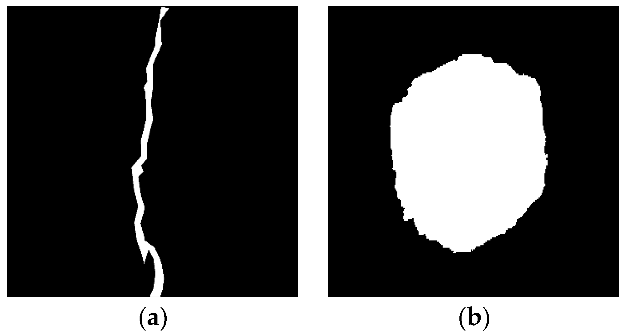
To address the complex background and noise interference of feeder road disease images, this study adopts a standardized preprocessing process: firstly, the crack and pothole images are grayscaled by the weighted average method, which weakens the background information and strengthens the disease features. Then the bilateral filtering algorithm is used to remove the noise, which improves the quality of the images while retaining the details of the crack edges and pothole contours. Finally, the diseased areas are binary-separated from the background by Otsu threshold segmentation, which obtains a binary separation between the diseased areas and the background [53]. Otsu threshold segmentation [54] is used to separate the diseased area and the background, and a clear binarized image is obtained, as shown in Figure 20. For the crack image, the morphological open operation is used to eliminate the slight noise, and the medial-axis transformation extracts the skeleton. For the pothole image, the morphological closed operation is used to fill the internal gaps to ensure the integrity of the contour of the diseased area [55], which lays the foundation for the subsequent computational analysis.

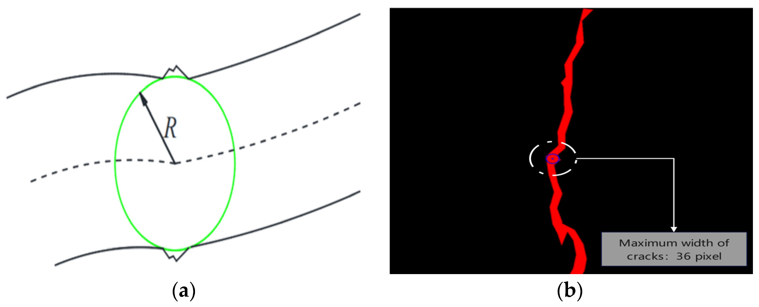
The center skeleton method measures crack width through geometric fitting and edge search. Based on the preprocessed binarized image, the crack skeleton is extracted by the medial-axis transformation, the centerline pixel coordinates are obtained, and the crack centerline is fitted based on the least-squares method. The normal vector is calculated for each point on the centerline, and the edges of the crack are searched along the direction of the normal vector; the maximum distance at the point is recorded as the local width, and the maximum value is taken as the maximum width of the crack after traversing all the points. In order to reduce the influence of edge roughness on the measurement, a geometric fitting strategy is used: based on the preprocessed binary map, the crack contour is extracted by OpenCV’s findcontours function, the maximum distance from each point to the edge within the contour is calculated by using the pointpolygontest function, the center and radius of the internal tangent circle are determined, as shown in Figure 21a, and the diameter of the circle is used as the width of the crack. As shown in Figure 21b, the maximum width measured by the center-skeleton method is 36 pixel values. The actual width is 2.916 mm after being converted using the camera calibration scale (0.081:1). With the accuracy of 0.01 mm vernier calipers on the crack width of manual measurement, in order to reduce the measurement of the error brought about by the need to repeat the measurement of the crack width of ten times, take the average value of 2.97 mm as the final width of the crack. The error mainly originates from the deviation in the normal vector estimation caused by the irregularity of the crack edge.

For potholes and other irregular diseases, the pixel occupancy method is used to quantify the area: after obtaining the outline of the complete diseased area through preprocessing, traverse all the pixels of the image, count the diseased area (white pixels) and the background area (black pixels), and calculate the degree of damage according to Equation (15).

$$Percentage of diseased area={\displaystyle \frac{Number of pixels in the disease area}{Total number of pixels in the whole image}}\times 100\%$$

(15)

As shown in

Table 6. Pothole area calculation results.

Pixel Distribution Statistical Indicators	Numerical Value
Total number of pixels	307,200
Total number of white pixels	87,908
Percentage of white pixels	28.62%
Total number of black pixels	219,292
Percentage of black pixels	71.38%

, the total number of pixel points is 30.7200, and the total number of pixel points in the diseased area is 87,908, accounting for 28.62%. The experimental results show that the proposed calculation method can effectively quantify the crack width and pothole area, and the calculation results are basically consistent with the measured data.

4. Conclusions

In response to the issue of the accuracy of feeder road disease detection being susceptible to the influence of concealment by weeds, tree shadows, and fallen leaves. Additionally, the change in disease morphology complicates identification, so an improved Rural-YOLO11 feeder disease detection algorithm is proposed. SAConv and C2PSA_CAA modules were introduced into the backbone network, the multi-channel and spatial attention (MCSAttention) was constructed during the feature fusion process, and finally, the initial loss function was replaced with WIoU v3. The proposed algorithm can extract disease information at a deeper level and adaptively adjust the weights of the feature map to suppress the influence of background features.

The proposed algorithm is effectively trained and tested using the RDD2022 dataset. The results showed that the improved Rural-YOLO model had increased precision by 2.4% and map₅₀ by 7.8% compared to the YOLOv11n model. In addition, recall increased by 8.4%, and model computation decreased by 21%. Through the testing and validation of the model in combination with the ablation experiment, comparison experiments, and generalization experiment, the results confirmed the timeliness and accuracy of the model, which also demonstrated strong generalization capabilities. Finally, quantitative experiments were conducted to calculate the percentage of crack width and pothole area, and the results were used as a reference for further damage assessment.

The detection results in the test set of images showed that compared to the YOLOv11n algorithm, the proposed Rural-YOLO disease detection algorithm showed higher confidence in various complex scenarios and had very few misdetections and omissions in the results, which effectively improved the algorithm’s adaptability in feeder disease detection.

However, road disease detection often encounters more complex environments, especially under severe weather conditions. Future research will focus on calculating information such as the depth of feeder road disease, significantly improving the system’s adaptability under adverse weather conditions, and proposing the development of intelligent detection terminals with real-time weather adaptability in response to project implementation needs. This will facilitate demonstrating the research results in highway inspection and farmland monitoring scenarios.