

Quad-Frequency Wide-Lane, Narrow-Lane and Hatch–Melbourne–Wübbena Combinations: The Beidou Case

Abstract

1. Introduction
2. Synthetic Meta-Signal Measurement Reconstruction
3. Quad-Frequency Narrow and Wide-Lane Combinations
4. Hatch–Melbourne–Wübbena Combinations
5. The Beidou Case
6. Material and Methods
7. Results
7.1. Quad-Frequency HMW Combinations
7.2. Wide-Lane Carrier Phase Combinations
8. Discussion
9. Conclusions
Author Contributions
Funding
Informed Consent Statement
Data Availability Statement
Conflicts of Interest
References
- Geng, J.; Guo, J. Beyond three frequencies: An extendable model for single-epoch decimeter-level point positioning by exploiting Galileo and BeiDou-3 signals. J. Geod. 2020, 94, 14. [Google Scholar] [CrossRef]
- Odijk, D.; Teunissen, P.J.G.; Tiberius, C.C.J.M. Triple-frequency ionosphere-free phase combinations for ambiguity resolution. In Proceedings of the European Navigation Conference ENC-GNSS, Copenhagen, Denmark, 27–30 May 2002; pp. 1–10. [Google Scholar]
- Odijk, D. Ionosphere-Free Phase Combinations for Modernized GPS. J. Surv. Eng. 2003, 129, 165–173. [Google Scholar] [CrossRef]
- Li, B. Review of triple-frequency GNSS: Ambiguity resolution, benefits and challenges. J. Glob. Position. Syst. 2018, 16, 1. [Google Scholar] [CrossRef]
- Li, B.; Li, Z.; Zhang, Z.; Tan, Y. ERTK: Extra-wide-lane RTK of triple-frequency GNSS signals. J. Geod. 2017, 91, 1031–1047. [Google Scholar] [CrossRef]
- Liu, L.; Pan, S.; Gao, W.; Ma, C.; Tao, J.; Zhao, Q. Assessment of Quad-Frequency Long-Baseline Positioning with BeiDou-3 and Galileo Observations. Remote Sens. 2021, 13, 1551. [Google Scholar] [CrossRef]
- Ji, S.; Liu, G.; Weng, D.; Wang, Z.; He, K.; Chen, W. Single-Epoch Ambiguity Resolution of a Large-Scale CORS Network with Multi-Frequency and Multi-Constellation GNSS. Remote Sens. 2022, 14, 3819. [Google Scholar] [CrossRef]
- Li, B.; Zhang, Z.; Miao, W.; Chen, G. Improved precise positioning with BDS-3 quad-frequency signals. Satell. Navig. 2020, 1, 30. [Google Scholar] [CrossRef]
- Zhang, Z.; Li, B.; He, X.; Zhang, Z.; Miao, W. Models, methods and assessment of four-frequency carrier ambiguity resolution for BeiDou-3 observations. GPS Solut. 2020, 24, 96. [Google Scholar] [CrossRef]
- Zhao, Q.; Pan, S.; Gao, W.; Wu, B. Multi-GNSS Fast Precise Point Positioning with Multi-Frequency Uncombined Model and Cascading Ambiguity Resolution. Math. Probl. Eng. 2022, 2022, 3478332. [Google Scholar] [CrossRef]
- Li, B.; Feng, Y.; Gao, W.; Li, Z. Real-time kinematic positioning over long baselines using triple-frequency BeiDou signals. IEEE Trans. Aerosp. Electron. Syst. 2015, 51, 3254–3269. [Google Scholar] [CrossRef]
- European Union. Galileo Open Service Signal-in-Space Interface Control Document (OS SIS ICD); Technical Report 2.1; European Union: Brussels, Belgium, 2023. [Google Scholar] [CrossRef]
- Lu, M.; Li, W.; Yao, Z.; Cui, X. Overview of BDS III new signals. NAVIGATION J. Inst. Navig. 2019, 66, 19–35. [Google Scholar] [CrossRef]
- Cocard, M.; Bourgon, S.; Kamali, O.; Collins, P. A systematic investigation of optimal carrier-phase combinations for modernized triple-frequency GPS. J. Geod. 2008, 82, 555–564. [Google Scholar] [CrossRef]
- Gao, W.; Liu, L.; Qiao, L.; Pan, S. Using Galileo and BDS-3 Quad-Frequency Signals for Long-Baseline Instantaneous Decimeter-Level Positioning. Math. Probl. Eng. 2021, 2021, 6558543. [Google Scholar] [CrossRef]
- Tang, W.; Deng, C.; Shi, C.; Liu, J. Triple-frequency carrier ambiguity resolution for Beidou navigation satellite system. GPS Solut. 2014, 18, 335–344. [Google Scholar] [CrossRef]
- Deng, J.; Zhang, A.; Zhu, N.; Ke, F. Extra-Wide Lane Ambiguity Resolution and Validation for a Single Epoch Based on the Triple-Frequency BeiDou Navigation Satellite System. Sensors 2020, 20, 1534. [Google Scholar] [CrossRef]
- Borio, D.; Gioia, C. Reconstructing GNSS Meta-Signal Observations Using Sideband Measurements. NAVIGATION 2023, 70, navi.558. [Google Scholar] [CrossRef]
- Borio, D.; Gioia, C. Synthetic Meta-Signal Observations: The Beidou Case. Sensors 2024, 24, 87. [Google Scholar] [CrossRef]
- Borio, D.; Susi, M.; Wezka, K. Meta-Signal Inspired Quad-Frequency GNSS Measurement Combinations. In Proceedings of the 37th International Technical Meeting of the Satellite Division of The Institute of Navigation (ION GNSS+), Baltimore, MD, USA, 16–20 September 2024; pp. 2203–2217. [Google Scholar] [CrossRef]
- Bolla, P.; Nurmi, J.; Won, J.; Lohan, E.S. Joint Tracking of Multiple Frequency Signals from the same GNSS satellite. In Proceedings of the International Conference on Localization and GNSS (ICL-GNSS), Guimaraes, Portugal, 26–28 June 2018; pp. 1–6. [Google Scholar] [CrossRef]
- Tian, Z.; Cui, X.; Liu, G.; Lu, M. LPRA-DBT: Low-Processing-Rate Asymmetrical Dual-Band Tracking Method for BDS-3 B1I and B1C Composite Signal. In Proceedings of the International Technical Meeting of The Institute of Navigation, Long Beach, CA, USA, 25–27 January 2022; pp. 1027–1038. [Google Scholar] [CrossRef]
- Yin, H.; Morton, Y.; Carroll, M. Implementation and Performance Analysis of a Multi-frequency GPS Signal Tracking Algorithm. In Proceedings of the 27th International Technical Meeting of the Satellite Division of The Institute of Navigation (ION GNSS+ 2014), Tampa, FL, USA, 8–12 September 2014; pp. 2747–2753. [Google Scholar]
- Issler, J.L.; Paonni, M.; Eissfeller, B. Toward centimetric positioning thanks to L- and S-Band GNSS and to meta-GNSS signals. In Proceedings of the ESA Workshop on Satellite Navigation Technologies and European Workshop on GNSS Signals and Signal Processing (NAVITEC), 8–10 December 2010; pp. 1–8. [Google Scholar] [CrossRef]
- Borio, D. Bicomplex Representation and Processing of GNSS Signals. NAVIGATION J. Inst. Navig. 2023, 70, navi.621. [Google Scholar] [CrossRef]
- Hatch, R. The synergism of GPS code and carrier measurements. In Proceedings of the Third International Symposium on Satellite Doppler Positioning, Las Cruces, NM, USA, 8–12 February 1982; pp. 1213–1231. [Google Scholar]
- Melbourne, W.G. The case for ranging in GPS-based geodeticsystems. In Proceedings of the First International Symposium on Precise Positioning with the Global Positioning System, Rockville, MD, USA, 15–19 April 1985; pp. 373–386. [Google Scholar]
- Wübbena, G. Software developments for geodetic positioning with GPS using TI 4100 code and carrier measurements. In Proceedings of the First International Symposium on Precise Positioning with the Global Positioning System, Rockville, MD, USA, 15–19 April 1985; pp. 403–412. [Google Scholar]
- Borio, D. A General Multi-Dimensional GNSS Signal Processing Scheme Based on Multicomplex Numbers. In Proceedings of the 37th International Technical Meeting of the Satellite Division of The Institute of Navigation (ION GNSS+), Baltimore, MD, USA, 16–20 September 2024; pp. 2904–2925. [Google Scholar] [CrossRef]
- Yarlagadda, R.K.R.; Hershey, J.E. Hadamard Matrix Analysis and Synthesis; The Springer International Series in Engineering and Computer Science; Springer: New York, NY, USA, 1997. [Google Scholar] [CrossRef]
- Zhang, X.; He, X.; Liu, W. Characteristics of systematic errors in the BDS Hatch–Melbourne–Wübbena combination and its influenceon wide-lane ambiguity resolution. GPS Solut. 2017, 21, 265–277. [Google Scholar] [CrossRef]
- de Bakker, P.F.; Tiberius, C.C.J.M.; van der Marel, H.; van Bree, R.J.P. Short and zero baseline analysis of GPS L1 C/A, L5Q, GIOVE E1B, and E5aQ signals. GPS Solut. 2011, 16, 53–64. [Google Scholar] [CrossRef]
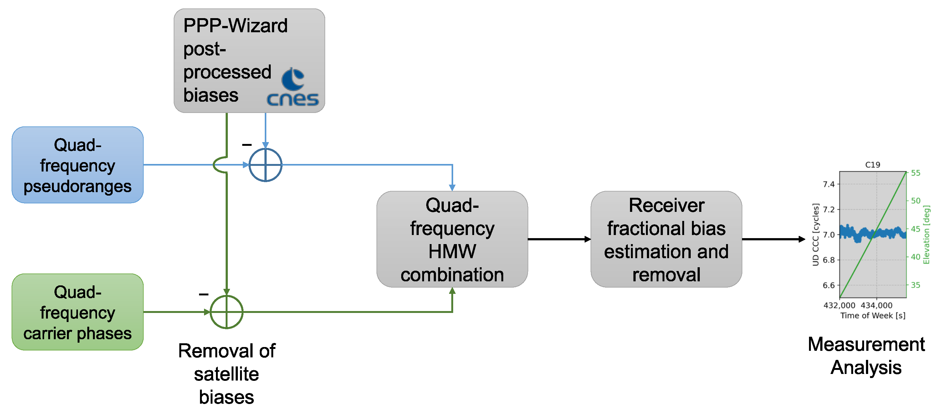
- Laurichesse, D.; Privat, A. An Open-source PPP Client Implementation for the CNES PPP-WIZARD Demonstrator. In Proceedings of the 28th International Technical Meeting of the Satellite Division of The Institute of Navigation (ION GNSS+), Tampa, FL, USA, 14–18 September 2015; pp. 2780–2789. [Google Scholar]
- Gazzino, C.; Blot, A.; Bernadotte, E.; Jayle, T.; Laymand, M.; Lelarge, N.; Lacabanne, A.; Laurichesse, D. The CNES Solutions for Improving the Positioning Accuracy with Post-Processed Phase Biases, a Snapshot Mode, and High-Frequency Doppler Measurements Embedded in Recent Advances of the PPP-WIZARD Demonstrator. Remote Sens. 2023, 15, 4231. [Google Scholar] [CrossRef]
- Gazzino, C.; Lelarge, N. A Cascading Approach for Multi-Frequency Widelanes and Extra-Widelanes Carrier Phase Integer Ambiguity Resolution. In Proceedings of the 37th International Technical Meeting of the Satellite Division of The Institute of Navigation (ION GNSS+), Baltimore, MD, USA, 16–20 September 2024; pp. 2136–2150. [Google Scholar] [CrossRef]
- Lestarquit, L.; Artaud, G.; Issler, J.L. AltBOC for Dummies or Everything You Always Wanted To Know About AltBOC. In Proceedings of the 21st International Technical Meeting of the Satellite Division of The Institute of Navigation (ION GNSS 2008), Savannah, GA, USA, 16–19 September 2008; pp. 961–970. [Google Scholar]
- Yao, Z.; Zhang, J.; Lu, M. ACE-BOC: Dual-frequency constant envelope multiplexing for satellite navigation. IEEE Trans. Aerosp. Electron. Syst. 2016, 52, 466–485. [Google Scholar] [CrossRef]
- Di Grazia, D.; Pisoni, F.; Gogliettino, G.; Gioia, C.; Borio, D. Putting the Synthetic GNSS Meta-signal Paradigm into Practice: Application to Automotive Market Devices. Eng. Proc. 2025, 88, 30. [Google Scholar] [CrossRef]
- Gao, Y.; Yao, Z.; Lu, M. High-precision unambiguous tracking technique for BDS B1 wideband composite signal. NAVIGATION 2020, 67, 633–650. [Google Scholar] [CrossRef]
- Wang, C.; Cui, X.; Ma, T.; Zhao, S.; Lu, M. Asymmetric Dual-Band Tracking Technique for Optimal Joint Processing of BDS B1I and B1C Signals. Sensors 2017, 17, 2360. [Google Scholar] [CrossRef]
- Beck, F.C.; Enneking, C.; Thölert, S.; Meurer, M. Galileo Performance Improvements Employing Meta-Signals—Robustness Analysis against Payload and Receiver Distortions. Eng. Proc. 2023, 54, 4. [Google Scholar] [CrossRef]
- de Bakker, P.F.; van der Marel, H.; Tiberius, C.C.J.M. Geometry-free undifferenced, single and double differenced analysis of single frequency GPS, EGNOS and GIOVE-A/B measurements. GPS Solut. 2009, 13, 305–314. [Google Scholar] [CrossRef]
- Schaer, S. SINEX BIAS—Solution (Software/Technique) INdependent EXchange Format for GNSS BIASes. 2016. Available online: https://files.igs.org/pub/data/format/sinex_bias_100.pdf (accessed on 1 February 2025).


| Combination | Weights | a | b | c | d |
|---|---|---|---|---|---|
| 1 | 2 | 3 | 4 | ||
| 1 | 3 | 2 | 4 | ||
| 1 | 2 | 4 | 3 |
| Signal/Combination | Frequency (MHz) | Wavelength (Meters) |
|---|---|---|
| B1C | 1575.42 | 0.19 |
| B1I | 1561.098 | 0.192 |
| B3I | 1268.52 | 0.236 |
| B2b | 1207.14 | 0.248 |
| B2a | 1176.45 | 0.255 |
| B1C − B1I | 14.322 | 20.932 |
| B2b − B2a | 30.69 | 9.768 |
| B3I − B2b | 61.38 | 4.884 |
| B3I − B2a | 92.07 | 3.256 |
| B1I − B3I | 292.578 | 1.025 |
| B1C − B3I | 306.9 | 0.977 |
| Conf. 1, B3I excluded | ||
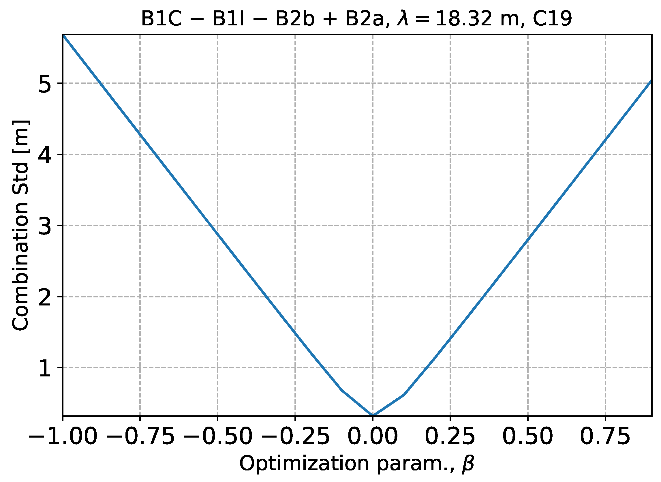
| B1C − B1I − B2b + B2a | 16.368 | 18.316 |
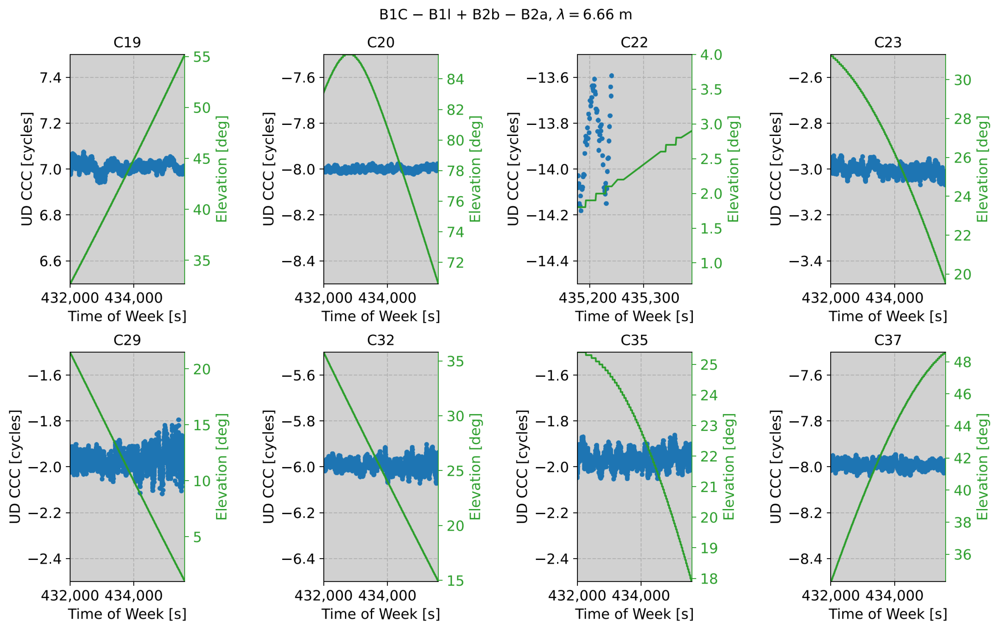
| B1C − B1I + B2b − B2a | 45.012 | 6.66 |
| B1C + B1I − B2b − B2a | 752.928 | 0.398 |
| Conf. 2, B1I excluded | ||
| B1C − B3I − B2b + B2a | 276.21 | 1.085 |
| B1C − B3I + B2b − B2a | 337.59 | 0.888 |
| B1C + B3I − B2b − B2a | 460.35 | 0.651 |
| Conf. 3, B1C excluded | ||
| B1I − B3I − B2b + B2a | 261.888 | 1.145 |
| B1I − B3I + B2b − B2a | 323.268 | 0.927 |
| B1I + B3I − B2b − B2a | 446.028 | 0.672 |
| Conf. 4, B2b excluded | ||
| B1C − B1I − B3I + B2a | 77.748 | 3.856 |
| B1C − B1I + B3I − B2a | 106.392 | 2.819 |
| B1C + B1I − B3I − B2a | 691.548 | 0.434 |
| Conf. 5, B2a excluded | ||
| B1C − B1I − B3I + B2b | 47.058 | 6.371 |
| B1C − B1I + B3I − B2b | 75.702 | 3.960 |
| B1C + B1I − B3I − B2b | 660.858 | 0.454 |
| Component | Specification |
|---|---|
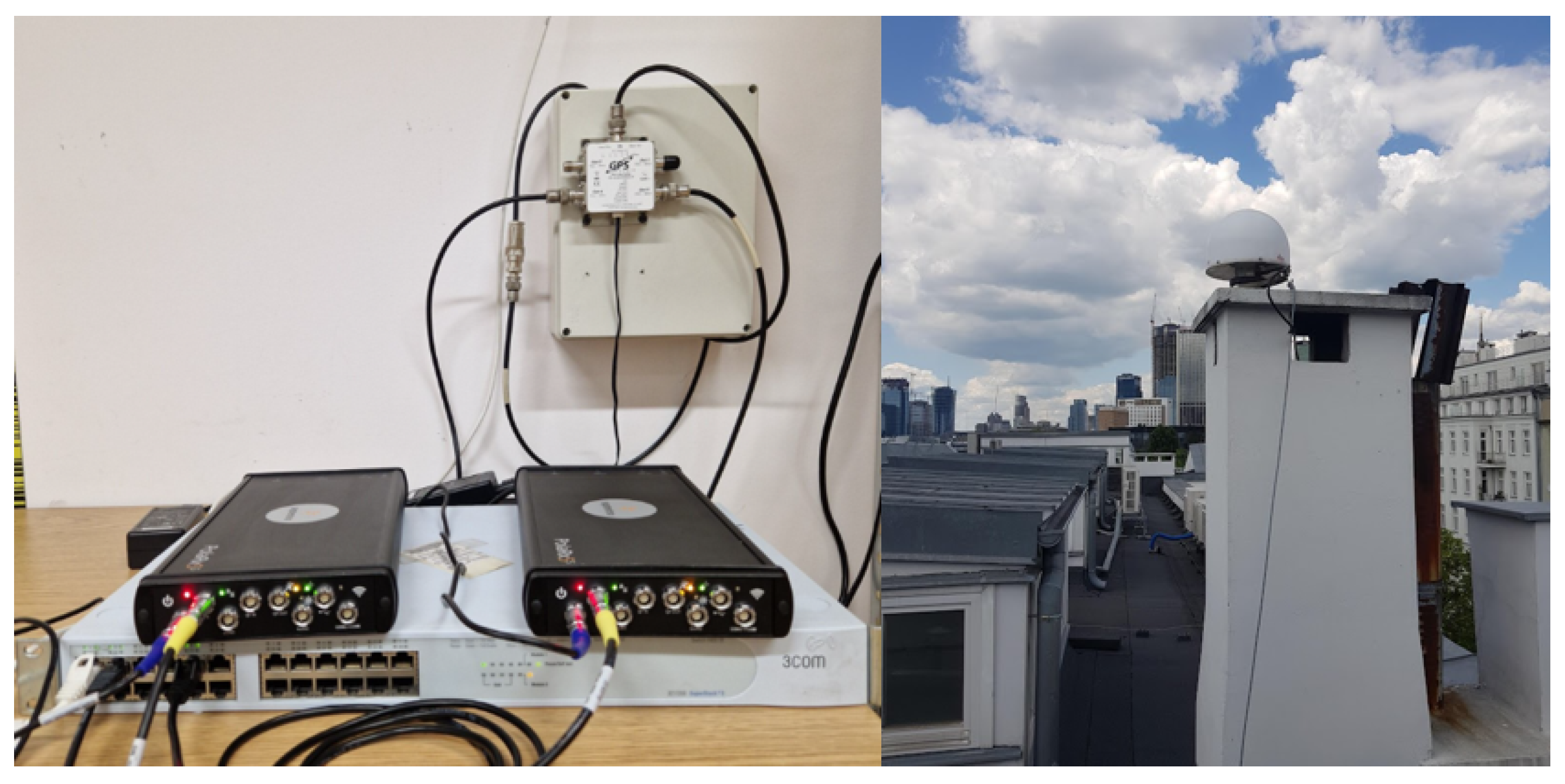
| Receiver | Septentrio PolaRx5S, (Septentrio, Leuven, Belgium) |
| Antenna | Leica AT504, (Leica Geosystems, Heerbrugg, Switzerland) |
| GNSS Spiter | GPS source (S14) |
| Antenna location | 52°13′15″ N, 21°00′37″ E |
| PRN | Fractional Mean (Cycles) | Standard Dev. (Cycles) |
|---|---|---|
| m | ||
| 19 | ||
| 20 | ||
| 22 | ||
| 23 | ||
| 29 | ||
| 32 | ||
| 35 | ||
| 37 | ||
| m | ||
| 19 | ||
| 20 | ||
| 22 | ||
| 23 | ||
| 29 | ||
| 32 | ||
| 35 | ||
| 37 | ||
| m | ||
| 19 | ||
| 20 | ||
| 22 | ||
| 23 | ||
| 29 | ||
| 32 | ||
| 35 | ||
| 37 |
| PRN | Fractional Mean (Cycles) | Standard Dev. (Cycles) |
|---|---|---|
| m | ||
| 19 | ||
| 20 | ||
| 22 | ||
| 23 | ||
| 29 | ||
| 32 | ||
| 35 | ||
| 37 |
| PRN | Fractional Mean (Cycles) | Standard Dev. (Cycles) |
|---|---|---|
| m | ||
| 19 | ||
| 20 | ||
| 22 | ||
| 23 | ||
| 29 | ||
| 32 | ||
| 35 | ||
| 37 | ||
| m | ||
| 19 | ||
| 20 | ||
| 22 | ||
| 23 | ||
| 29 | ||
| 32 | ||
| 35 | ||
| 37 | ||
| m | ||
| 19 | ||
| 20 | ||
| 22 | ||
| 23 | ||
| 29 | ||
| 32 | ||
| 35 | ||
| 37 |
| PRN | Fractional Mean (Cycles) | Standard Dev. (Cycles) |
|---|---|---|
| m | ||
| 19 | ||
| 20 | ||
| 22 | ||
| 23 | ||
| 29 | ||
| 32 | ||
| 35 | ||
| 37 |
| PRN | Fractional Mean (Cycles) | Standard Dev. (Cycles) |
|---|---|---|
| m | ||
| 20 | ||
| 22 | ||
| 23 | ||
| 29 | ||
| 32 | ||
| 35 | ||
| 37 | ||
| m | ||
| 20 | ||
| 22 | ||
| 23 | ||
| 29 | ||
| 32 | ||
| 35 | ||
| 37 | ||
| m | ||
| 20 | ||
| 22 | ||
| 23 | ||
| 29 | ||
| 32 | ||
| 35 | ||
| 37 |
Disclaimer/Publisher’s Note: The statements, opinions and data contained in all publications are solely those of the individual author(s) and contributor(s) and not of MDPI and/or the editor(s). MDPI and/or the editor(s) disclaim responsibility for any injury to people or property resulting from any ideas, methods, instructions or products referred to in the content. |
© 2025 by the authors. Licensee MDPI, Basel, Switzerland. This article is an open access article distributed under the terms and conditions of the Creative Commons Attribution (CC BY) license (https://creativecommons.org/licenses/by/4.0/).
Share and Cite
Borio, D.; Susi, M.; Wȩzka, K. Quad-Frequency Wide-Lane, Narrow-Lane and Hatch–Melbourne–Wübbena Combinations: The Beidou Case. Electronics 2025, 14, 1805. https://doi.org/10.3390/electronics14091805
Borio D, Susi M, Wȩzka K. Quad-Frequency Wide-Lane, Narrow-Lane and Hatch–Melbourne–Wübbena Combinations: The Beidou Case. Electronics. 2025; 14(9):1805. https://doi.org/10.3390/electronics14091805
Chicago/Turabian StyleBorio, Daniele, Melania Susi, and Kinga Wȩzka. 2025. "Quad-Frequency Wide-Lane, Narrow-Lane and Hatch–Melbourne–Wübbena Combinations: The Beidou Case" Electronics 14, no. 9: 1805. https://doi.org/10.3390/electronics14091805
APA StyleBorio, D., Susi, M., & Wȩzka, K. (2025). Quad-Frequency Wide-Lane, Narrow-Lane and Hatch–Melbourne–Wübbena Combinations: The Beidou Case. Electronics, 14(9), 1805. https://doi.org/10.3390/electronics14091805