Evaluating GNSS Receiver Resilience: A Study on Simulation Environment Repeatability

Abstract

Global navigation satellite systems (GNSSs), with their ubiquitous coverage, have become a cornerstone of modern position, navigation, and timing (PNT) services. While their spread spectrum communication offers inherent, albeit partial, resilience against interference, GNSSs remain a prime target for malicious actors seeking to disrupt or degrade precise location and time synchronization. Jamming mitigation has been an active research area for over three decades. Despite diverse research efforts, a key weakness in the literature is the absence of rigorous, methodologically sound testing of proposed mitigation techniques in a controlled laboratory environment. This work addresses this deficiency by exploring the challenges of evaluating GNSS receiver performance and response under interference and by proposing a more robust methodological framework for result interpretation. We present a custom simulation environment that enables repeated, controlled measurements of GNSS receiver behavior under various jamming attacks, revealing discrepancies between expected performance and real-world observations. Using three low-cost receivers as a case study, we demonstrate the inherent uncertainty in the results, the unpredictable behavior of the receivers’ embedded software, and appropriate statistical analysis practices. A key contribution of this work is a publicly available dataset of extensive GNSS receiver response measurements acquired under controlled interference conditions using an advanced signal generation and a comprehensive satellite constellation simulator.

1. Introduction

Global navigation satellite systems are deeply embedded in our world, providing seamless navigation on our phones and supporting the complex operations of maritime, aviation, and energy systems [1]. Their precise timing, derived from atomic clocks onboard satellites, enables stable time synchronization for essential services, including financial trading, broadcasting centers, and advanced decentralized networks [2,3,4].

With four major constellations now operational (GPS, Galileo, BeiDou, and GLONASS), the number of users relying on GNSSs for positioning, navigation, and timing continues to expand [5]. However, this widespread dependence also introduces vulnerabilities [6]. As early as the 1970s, when GPS was initially designed, engineers anticipated potential interference, both intentional and unintentional [7]. To mitigate this, they employed spread spectrum techniques and, for added security, a military signal alongside the civilian one with much greater bandwidth and thus resistance to narrowband interference [8]. For two decades, the system proved remarkably robust, with interference primarily limited to military conflict zones or unintentional disruptions from early mobile phone networks [9]. Despite the increased resilience provided by multiple GNSS constellations, the widespread availability of low-cost, portable jammers, thanks to rapid semiconductor development, has created a new vulnerability [10]. Even simple, low-power devices can effectively disable a receiver’s positioning and timing functions [4]. These devices can overwhelm weak satellite signals, which are often close to the receiver’s noise floor, or saturate the sensitive low-noise amplifiers of active antenna circuitry [9,11,12,13,14].

While interference can be disruptive, it is not always catastrophic, provided we recognize when a receiver’s data are compromised. Researchers have developed various methods for detecting interference, ranging from monitoring amplifier gain stages to analyzing signal patterns [5,15,16]. Modern receivers can often identify strong jamming signals and adapt accordingly, using techniques like adaptive filtering or switching to alternative GNSS systems [17]. More subtle forms of interference, however, pose a greater challenge. These low-level jamming signals, which might originate from distant sources or be deliberately transmitted by malicious actors, can degrade positioning and timing accuracy without triggering automatic jamming detection mechanisms [18,19,20]. This allows them to disrupt operations without causing a complete system failure.

The escalating threat of GNSS jamming has seen a dramatic surge, with a staggering increase of over 500% in reported incidents during the second quarter of 2024 [21]. This spike, particularly prevalent among aircraft operators near conflict zones experiencing widespread GPS jamming, has yet again propelled studies of interference impacts on GNSS receivers to the forefront of research. While some investigations employ partial simulations, the majority of researchers opt for real-world observations [9,10,12,14,22]. However, these field studies are inherently limited by the dynamic nature of the environment. Factors such as fluctuating satellite positions, varying atmospheric conditions, and unpredictable ionospheric activity make repeatable measurements exceedingly difficult [23]. Consequently, the conclusions drawn from these observations often lack generalizability, as they are confined to specific scenarios and cannot be independently verified [24]. Furthermore, the variability in receiver software responses adds another layer of uncertainty to the analysis [25,26].

This research addresses the critical need to quantify the uncertainty in GNSS receiver software behavior under interference, particularly when operating near critical thresholds. By utilizing physical GNSS simulators under controlled laboratory conditions, we aim to overcome the limitations of real-world observations [27]. This methodology enables repeatable experiments, allowing for a rigorous assessment of the receiver software’s response to various interference types and power levels. Our findings reveal that, even within a controlled environment, the evaluation of interference effects presents significant challenges. We demonstrate that accurate assessments require a statistical approach, highlighting the inherent variability in receiver responses. This work aims to shift the paradigm in GNSS interference research, advocating for a more systematic and statistically robust methodology. By providing a controlled environment and repeatable measurements, this study sets a foundation for a more standardized approach to assessing GNSS receiver vulnerability [28].

The main contribution of this work lies in the proposed method for a statistically sound assessment of GNSS module response to disturbances. By applying this method to an extensive dataset acquired through statistically sound testing in a controlled environment, we clearly demonstrate the inherent unpredictability of GNSS receiver software’s responses, particularly when operating within the power limits of jamming signals. The publicly available dataset further supports this finding and is anticipated to be an invaluable resource for researchers developing and validating jamming detection and mitigation techniques, ultimately fostering a more statistically robust framework for evaluating GNSS receiver vulnerability to interference.

The article is structured in six sections. The Section 2 lays the groundwork by discussing the fundamentals of interference and its detection in GNSS receivers. The Section 3 details the methodology for statistically evaluating receiver responses. The Section 4 describes our laboratory setup, including its requirements and limitations. The Section 5 presents key measurement results that illustrate the challenges of interference assessment. Finally, the Section 6 discusses our findings and offers recommendations for future research in this area.

2. GNSS Jamming and Detection Mechanisms

2.1. Interference in GNSS Reception

The challenge of receiving signals from the global network of orbiting satellites is fundamentally rooted in an extremely poor signal-to-noise ratio. This degradation is primarily caused by the scattering of radio signals as they interact with water molecules in the Earth’s atmosphere. While directional antennas can significantly improve this ratio by focusing their main beam on a specific transmitter, as seen in satellite internet, or by maintaining a fixed orientation toward geostationary satellites, as in satellite television, these solutions are not universally applicable [4].

A major hurdle emerges when a system requires hemispherical Earth coverage while simultaneously managing signals from numerous satellites positioned at diverse angles relative to multiple ground users [29]. In such scenarios, directional antennas, which would normally enhance the signal-to-noise ratio, become impractical. To overcome the resulting signal degradation, GNSS designers implemented spread spectrum code [30]. This technique broadens the signal’s bandwidth far beyond the data’s minimum requirement, effectively spreading it. By employing code multiplexing and de-spreading at the receiver, the system gains inherent resistance to narrowband interference. This interference is transformed into benign noise during demodulation, provided it lacks substantial correlation with the authentic satellite signals [31].

Modern receiver architecture allows for the reliable reception of navigation data from all four major GNSS constellations—Galileo, BeiDou, GLONASS, and GPS—even in the presence of relatively strong unintentional interference [32]. Such interference often originates from the suboptimal operation of terrestrial systems, notably the saturated output stages of mobile telephony base stations attempting to maximize their range [33]. 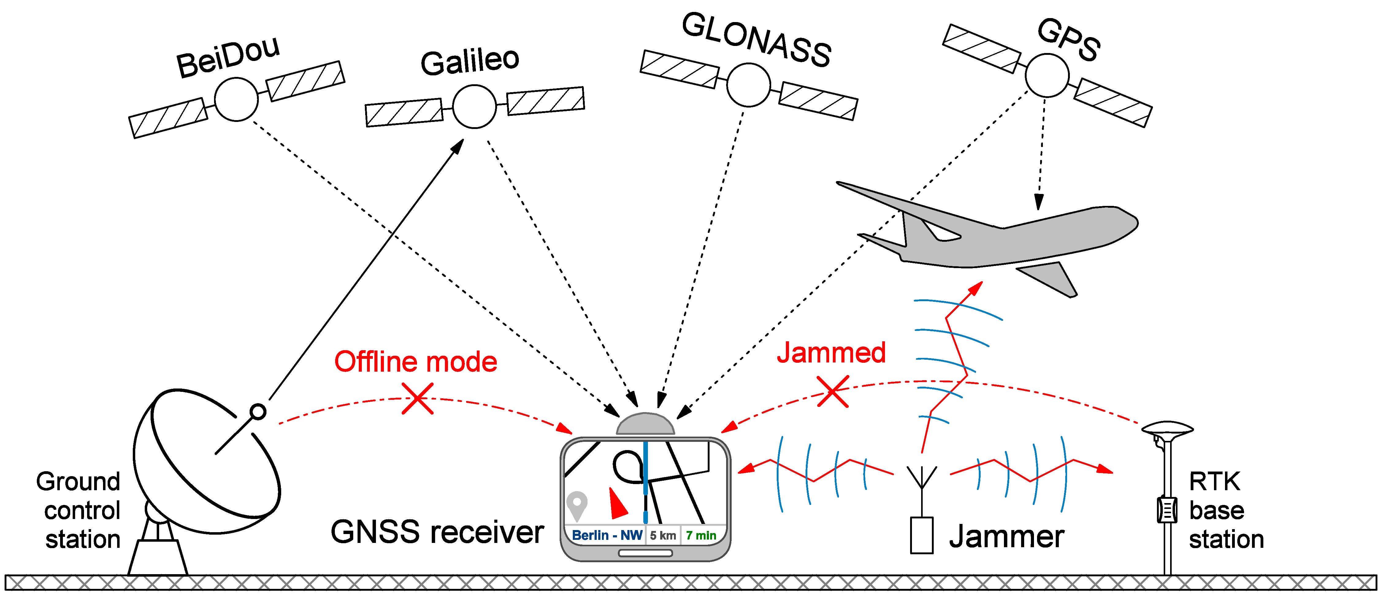However, the situation is markedly different with intentional jamming, which has become increasingly prevalent since the introduction of electronic tachographs in trucks [34]. Drivers seeking to conceal violations of driving time limits employ jammers to disrupt GNSS signal reception. A simple jammer, such as one designed for a 12 V cigarette lighter socket, can completely obscure GNSS signals within a range of tens of meters [35]. This has consequences beyond just the jammer user, endangering critical infrastructure such as airport systems and aircraft receivers (Figure 1) [36]. Intentional jamming typically involves transmitting directly at the carrier frequency of a specific GNSS system or randomly varying across the entire allocated frequency band, attempting to circumvent jamming detection systems. While GNSS receivers employ adaptive filtering and gain adjustments to counter jamming, sufficiently strong jamming signals can completely overwhelm the satellite signal during code de-spreading [37].

While a complete failure to de-spread a signal typically provides a clear indication of jamming conditions, more subtle disruptions can occur. A jammer might interfere with precise time synchronization without fully disabling signal reception, leading to inaccurate location calculations before the receiver software detects any deviations. To address these risks, researchers have developed countermeasures like ground station signal authentication and auxiliary RTK systems for precise positioning [6,38,39,40]. However, these solutions are also susceptible to disruption, as transmitting correction and authentication data over separate networks introduces additional vulnerabilities. Even kinematic auxiliary systems, such as gyroscopes and accelerometers, offer limited protection, especially during continuous motion. In such instances, the GNSS receiver, along with all of the components of its processing chain, constitutes an isolated system, relying solely on its software to interpret the situation and provide accurate positioning.

2.2. Receiver Internal Effects and Jammer Detection

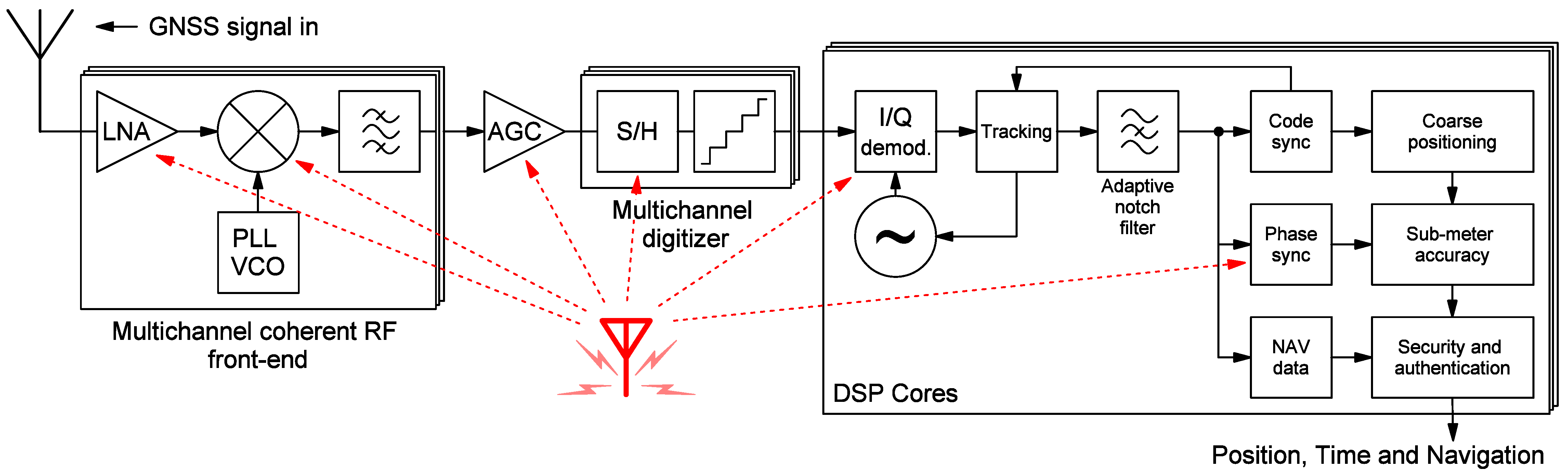
Modern GNSS receivers are designed to anticipate and adapt to interference. Figure 2 depicts a block diagram of a typical multi-frequency, multi-channel GNSS receiver, featuring an analog high-frequency front-end and digital signal processing (DSP) with associated software [41]. While adaptive notch filters within the DSP routine can effectively remove narrowband interference, they cannot prevent its initial impact on the earlier preprocessing stages.

The most critical weakness resides in the first low-noise amplifier (LNA), often built into the active antenna. This LNA, providing approximately 25 dB of gain, is vital for maximizing the receiver’s sensitivity. However, its need for an extremely low noise figure at high gain makes it only conditionally stable, easily disturbed by strong jamming signals. These signals drive the amplifier into unintended operating conditions, typically saturation, producing numerous intermodulation products [42]. These products, when combined with the subsequent mixing stage, generate unwanted responses in the output spectrum, resembling broadband noise—a noise that cannot be removed by de-spreading. Using narrowband antennas or SAW filters offers little relief, as they generally pass the entire GNSS spectrum, including the intentional jamming signals.

To address this issue, a passive antenna can be used, requiring the fixed LNA gain to be replaced with an automatic gain control (AGC) amplifier, a standard feature in modern GNSS receivers [43]. The AGC amplifier’s gain can be dynamically adjusted, enabling adaptive response to changing conditions. However, incorrect adjustments can significantly impair digital sampling before the DSP stage, especially if changes occur during the sampling process of the analog-to-digital converter’s sample and hold (S/H) circuit [44]. Furthermore, interference during I/Q demodulation, typically handled digitally, can also create problems. A substantial deviation from quadrature hinders accurate carrier phase synchronization, although this can be mitigated with appropriate countermeasures within DSP routines [45].

The receiver’s software constantly monitors these components and activates the appropriate response to interference. While the core architecture of modern GNSS receivers is largely standardized, significant differences arise in software implementation, particularly in DSP routines, calculation methods, and reactions to unexpected situations. GNSS receiver software is typically secured within the system using various cryptographic algorithms, preventing end-user modification or detailed analysis [41]. Moreover, the software’s behavior in response to identical, unforeseen interferences can fluctuate over time, leading to unpredictable adjustments to the AGC amplifier gain, adaptive filter settings, and I/Q quadrature correction. Given the absence of universal standards for interference response, manufacturers employ a wide range of proprietary solutions.

This research highlights that, even with consistent GNSS signal conditions and measurement durations, a receiver’s response to interference remains highly unpredictable due to its software. Therefore, simply observing receiver behavior in interference-rich environments is insufficient. Accurate evaluation demands repeated testing under controlled conditions, followed by thorough statistical analysis of the results.

3. Impacts of GNSS Variability

In practice, each GNSS receiver operates under unique conditions, dictated by its received signals, unless all receivers share a common antenna. Each receiver might detect different satellites from at least one of the four constellations globally available, each transmitting at varying power levels, following distinct orbital planes, and being at different stages of their operational lifespan. The signals then traverse the ionosphere (which fluctuates with solar activity) and may be reflected by natural or man-made structures before reaching the antenna. The receiver’s software must process and compensate for these variations to provide users with accurate time, position, heading, and speed information [41]. Remarkably, even when connected to a shared antenna and receiving identical signals, different GNSS receivers still yield varying results. Figure 3 illustrates this phenomenon, with measurements taken at a fixed location on June 10, 2024. Three distinct receivers, connected to a common signal source and thus operating under identical external conditions, were used. This figure shows the dispersion of position deviations around the reference location (46°02′55.6″ N 14°30′30.7″ E) over a four-hour observation period. The receivers operated in a completely offline mode, without connection to a backend network for RTK corrections or internet access for almanac downloads, and were subjected to an interference-free environment.

The results demonstrate the inherent variability of GNSS positioning. Even with a stationary receiver location, measurements fluctuate over time, and calculated positions differ significantly between receivers. As expected, newer receivers, such as the U-blox 10-Series, show considerably higher positioning accuracy compared to older models like the U-blox 6-Series. This improvement is primarily due to their ability to simultaneously receive signals from multiple systems and satellites. While deviation of the measurements from the true position cannot be entirely eliminated without auxiliary systems, the time-varying receiver position can be estimated by averaging time-based measurements and calculating the median, assuming the receiver is known to be stationary (black dots in Figure 3).

The complexity of this issue increases significantly when interference is introduced within the GNSS frequency range. Each receiver’s software will react to this interference, potentially by re-synchronizing satellites, switching to a different primary constellation, or attempting to digitally filter out the interfering signal. The exact response remains unpredictable due to the inaccessibility of the receiver’s source code. Consequently, the receiver’s unknown reaction to interference becomes an additional variable in the challenge of localization in jamming environments. An unpredictable response of a GNSS receiver to a disturbance is shown in Figure 4. To analyze this response, the problem’s complexity must first be reduced. While satellite movement and ionospheric variations are uncontrollable, the receiver can be transferred to a simulation environment. Here, a specific GNSS signal, including interference, can be precisely recreated and replayed. This eliminates the uncertainty of unpredictable environmental variables.

While a simulation allows for repeated measurements, unlike the unpredictable nature of real-world, time-varying positioning, a receiver’s response still presents uncertainties. However, if we consistently initialize the receiver to a known state and the GNSS simulator precisely replicates the signals, we can statistically analyze multiple measurements under identical conditions—an advantage impossible in live testing. Therefore, to thoroughly assess a receiver’s vulnerability to jamming, an automated system is essential. This system must feature the ability to reset the receiver to a defined initial state, a multi-frequency GNSS simulator capable of accurately reproducing all satellite constellation signals, a controllable jamming signal source, and an automated measurement processing software with statistical analysis code (the latter is detailed in Appendix A).

4. Automated Testbed

When jamming occurs, a receiver initiates procedures to mitigate its effects. However, the receiver’s response can vary slightly due to the multiple available jamming elimination methods and the receiver’s current signal processing step for position and time calculations. To characterize this response reliably, repeated measurements under jamming conditions are essential. To isolate the receiver’s behavior from dynamic real-world influences, we utilize a GNSS signal simulator.

This simulator employs mathematical models to recreate the received signal spectrum at a specified location. It simulates all relevant factors, including satellite orbital motion, ionospheric errors, signal degradation during transmission and reception, and potential transmission errors. The simulator generates a time sequence of raw I/Q samples, which are then fed to a high-frequency source with an output modulator to produce the desired simulated signals. This approach allows for repeatable testing under identical conditions, provided the source’s output power, frequency, and quadrature stability remain consistent.

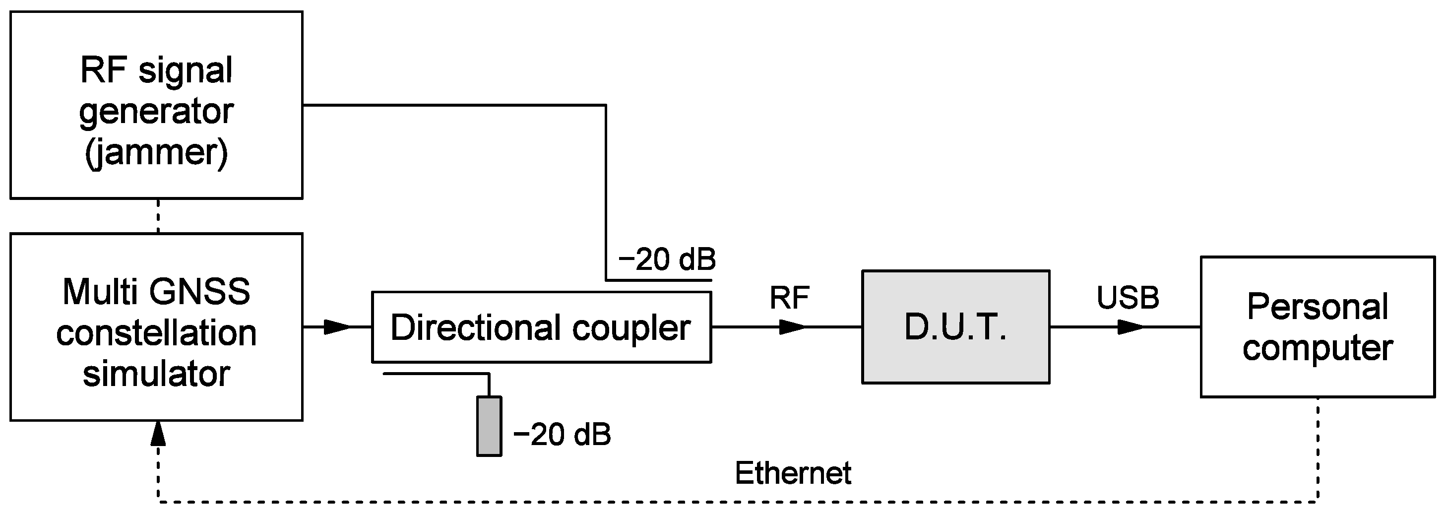
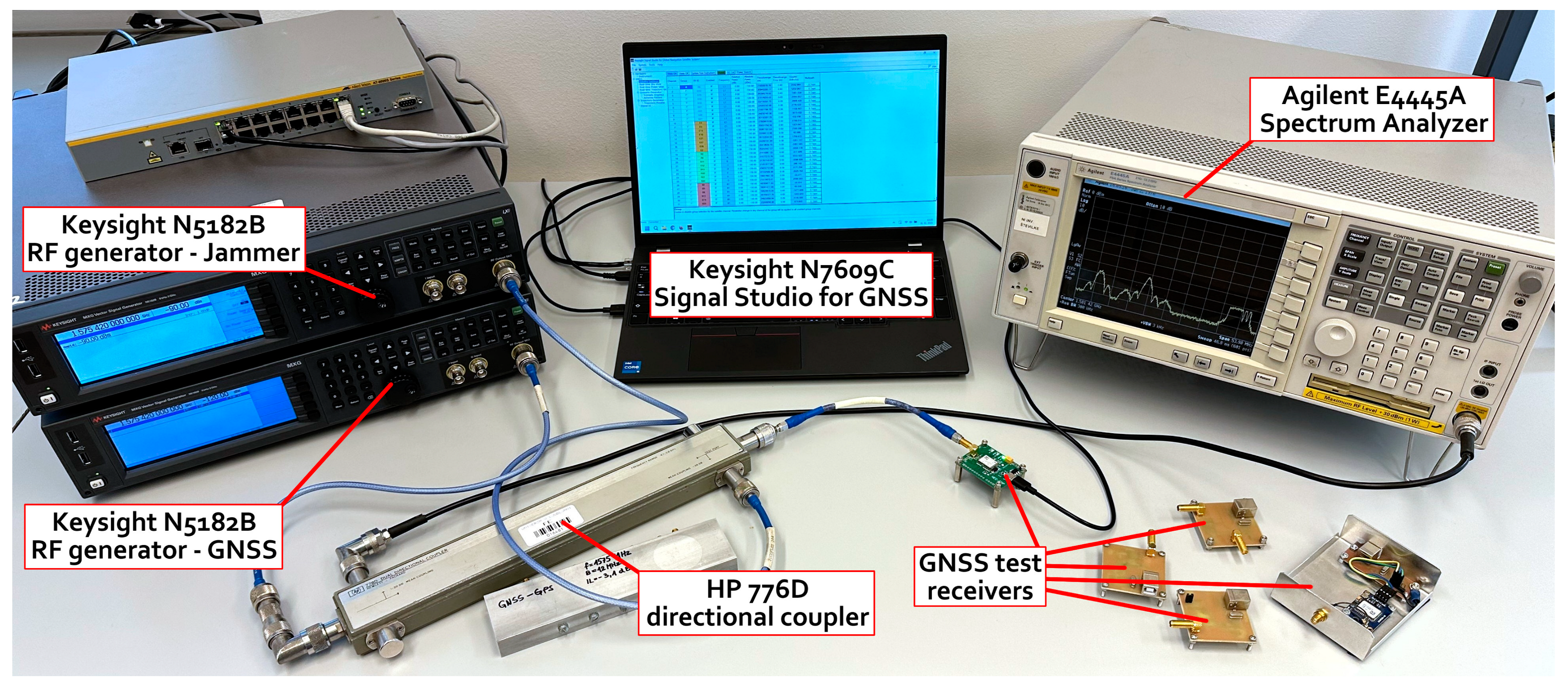
Laboratory tests have demonstrated that the setup depicted in Figure 5 provides the most reliable testing environment for receiver response assessment. The Keysight N7609C Signal Studio for Global Navigation Satellite Systems software generates the simulation waveforms, and the raw I/Q samples are then transferred to a Keysight N5182B high-frequency generator. This generator offers a wide power range (−137 dBm to 30 dBm), enabling precise control of the signal strength, thus eliminating the influence of the LNA amplifier. The GNSS signal is then routed through an HP 776D directional coupler, where an interfering signal, generated by a separate Keysight N5182B, is injected into the coupling connection. The unused port is terminated with a 50 Ω load. The combined signal is then fed to the GNSS receiver under test, and its output data are captured via USB on a personal computer. The directional coupler is crucial for preventing the interfering signal from distorting the GNSS simulator’s output spectrum, which would compromise the test’s integrity.

The personal computer software manages several concurrent tasks. It can initiate a cold start on the GNSS receiver, clearing its RAM and ensuring no residual data influence the test. Alternatively, the receiver’s power can be electronically cycled to guarantee a clean cold start. This is vital for observing the receiver’s response to sudden interference without the influence of prior data that might aid in positioning and error correction. The software also controls the GNSS simulator and jammer, executing pre-programmed scenarios with synchronized playback. This allows for precise timing of the jamming signal within the simulated environment. Finally, the software logs all received GNSS data, including NMEA sentences, along with simulation and jamming signal status information. Figure 6 shows a photograph of the measurement setup, which also includes an Ethernet switch for communication between the PC and the GNSS simulator/jammer and an Agilent E4445A Spectrum Analyzer for monitoring the output spectrum and estimating the signal-to-interference ratio.

Off-the-shelf GNSS receiver modules, specifically Ai-Thinker GP-01, U-blox NEO-6M (6-Series, GPS-only), and U-blox MAX-M10 (10-Series, multi-GNSS), were selected to validate the main research question. Testing an older generation receiver allows for a clearer illustration of the advantages of modern interference mitigation techniques and the benefits of utilizing multiple satellite navigation systems. Modules were then mounted onto custom-designed printed circuit boards to provide crucial additional functionalities not typically found in commercial products: the ability to completely remove power from the GNSS module (including disconnecting any NVRAM backup battery) and to issue a reset signal via USB commands. A USB-RS232 TTL integrated circuit facilitated serial communication and control over both the power supply and the reset signals. This setup granted the PC-based control software complete authority over the module’s state, enabling a true cold start condition for each measurement, ensuring consistent initial conditions across all repetitions. The choice of these low-cost receivers serves to demonstrate the significant impact of jamming, a factor often underestimated by researchers whose primary focus is not GNSS, leading them to consider more expensive, potentially more robust receivers as unnecessary. Furthermore, low-cost variants are prevalent in everyday consumer electronics, from drones to vehicle navigation systems. Utilizing these readily available modules allows for a direct comparison between single-frequency receivers, a comparison that would necessitate a redesign of the jamming scenarios to incorporate additional frequency bands if more expensive, often dual-frequency, receivers were used.

To evaluate the receiver response to interference, a comprehensive test involving three receivers subjected to various interference scenarios was conducted using a simulated static GNSS position (46°02′55.6″ N 14°30′30.7″ E) with satellite almanacs and ephemerides from June 10, 2024, 12:00 CET. Simulating a static location via a GNSS simulator was a deliberate choice, crucial for the clarity of this research by eliminating additional variables. In dynamic movement scenarios, GNSS modules can leverage external MEMS accelerometers to predict heading and speed, delaying the noticeable impact of jamming. This additional complexity would obscure the core interference effects that this research aims to communicate. Furthermore, static locations represent real-world critical applications, such as reference GNSS networks in geodesy for RTK correction systems and slow-moving objects like shipyard cranes, which require robust operation in jamming-free environments.

Each receiver underwent 50 repeated measurements for different interference conditions. Before measurement, the GNSS module’s power supply was cycled via program commands to ensure a consistent cold start state, devoid of almanac data, visible satellites, and code synchronization. The simulation began with the playback of the I/Q samples and simultaneous power-up of the GNSS module. The receivers were allowed 180 s to achieve their initial 3D position fix, a duration exceeding their typical acquisition time to provide a safety margin. Following this, NMEA sentences, representing the receiver’s output, were recorded at a 1 Hz frequency interval.

Subsequently, an external jammer was activated for 100 s (within 280 s of the simulation’s start) and then deactivated. The receiver’s data recording continued for an additional 80 s after the jammer was turned off. The simulation concluded, data recording ceased, and the receiver was reset to its initial state, clearing its memory before the next repetition. This cycle was repeated 50 times for each interference type and power level.

The evaluation of receiver response involved three distinct types of interference: a continuous wave (CW) jammer precisely at the GPS L1 center frequency of 1575.42 MHz; a three-frequency jammer at 1575.42 MHz with offsets of ± 735 kHz; and frequency-modulated (FM) interference centered at 1575.42 MHz, featuring an 8 MHz deviation and a 1 kHz modulation rate. Each of these interference types was tested across six power levels, spanning −70 dBm to −45 dBm. To establish a baseline, 50 measurements were also conducted without any interference, ensuring that any residual signal from the RF jammer remained below −155 dBm. The signal power level from the GNSS simulator was set to −130 dBm (representing the first lobe power of the BPSK modulation spectrum) and validated with a spectrum analyzer before any measurements were taken.

5. Results

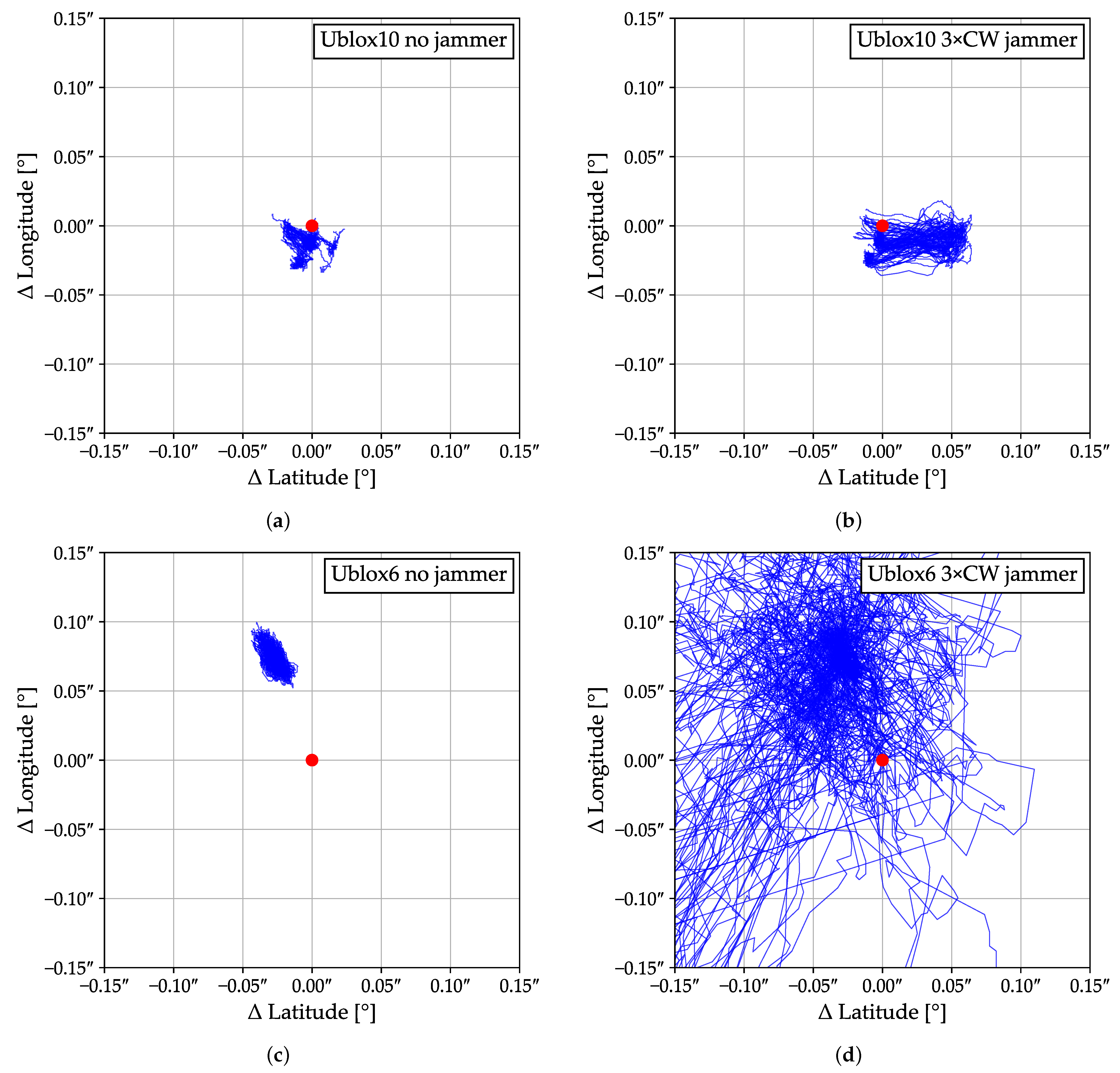
The results of the GNSS receivers’ responses to interference, in terms of position determination, can be displayed in various ways, with the events being most easily visualized using the display in Figure 7. Graphs a and b depict the U-blox 10-Series, while c and d show the U-blox 6-Series. Each graph displays all 50 measurement repetitions at once, with the red dot representing the reference position generated by the GNSS simulator software and replayed with the RF generator. The blue curve illustrates the post-processed position deviation (angular minutes for latitude and longitude). This deviation was calculated by comparing the GNSS receivers’ output to a known, simulated location (used by the RF generator), not directly computed by the receiver itself.

While the static display in Figure 7 reveals the magnitude of positional errors, it fails to capture the dynamic temporal response of the receiver, particularly its reaction to disturbances relative to its prior state. To address this, Figure 8 presents the results plotted against a time axis.

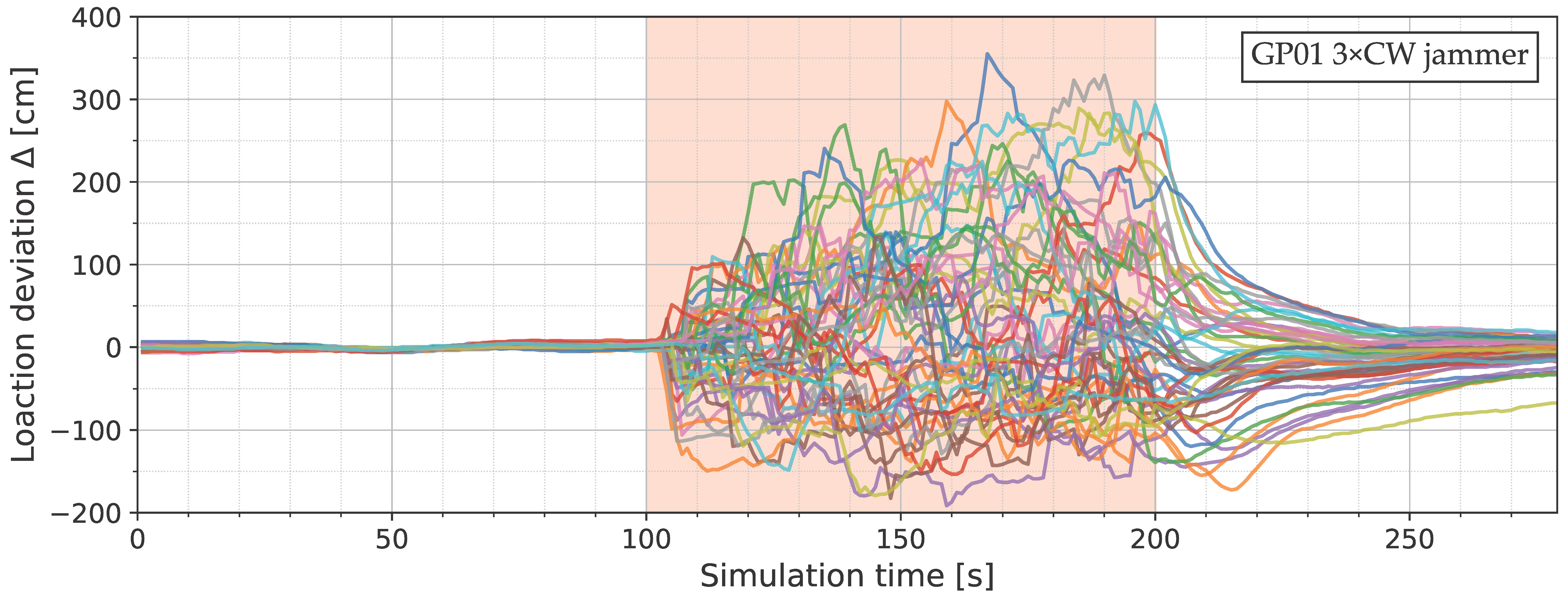
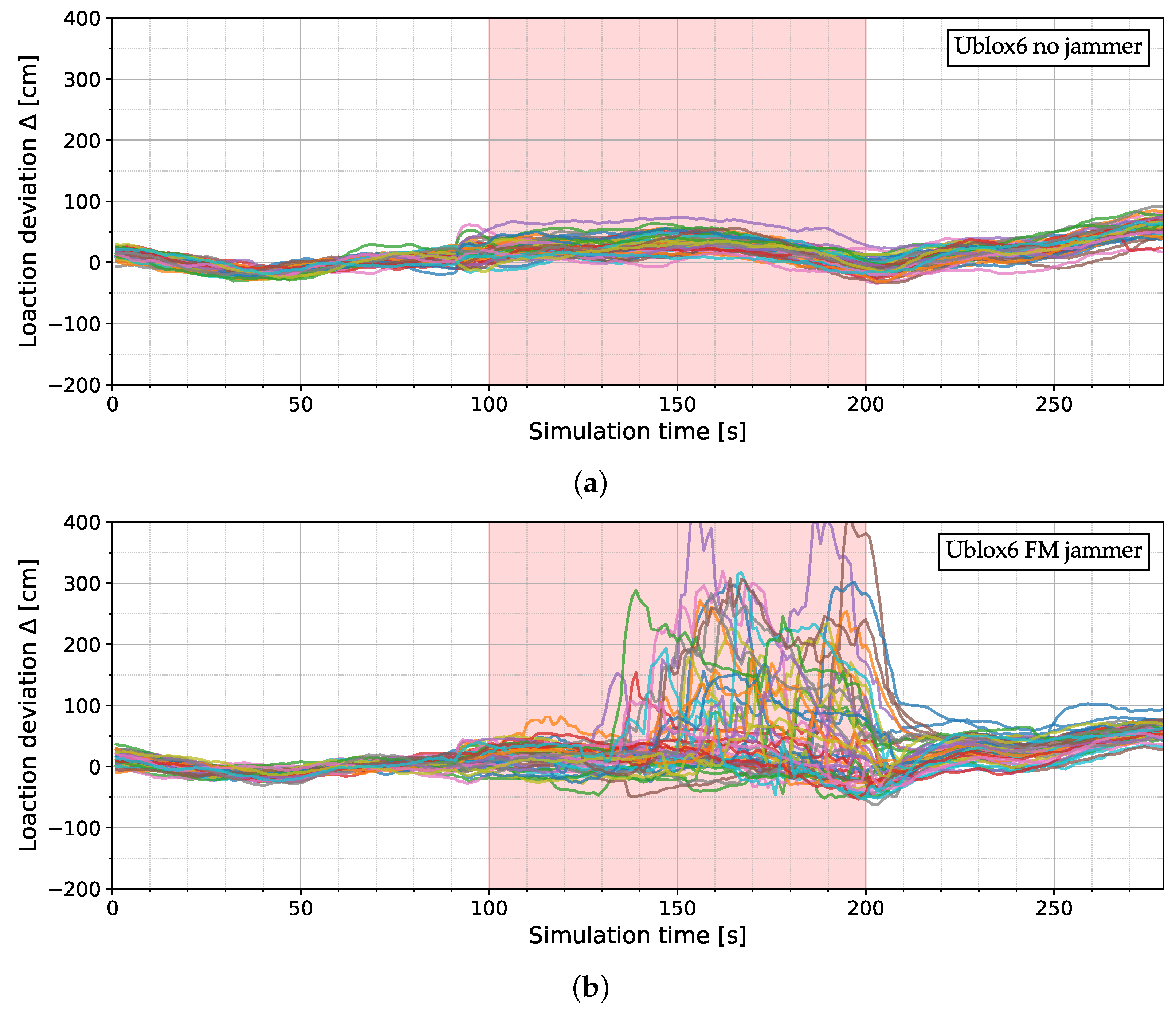
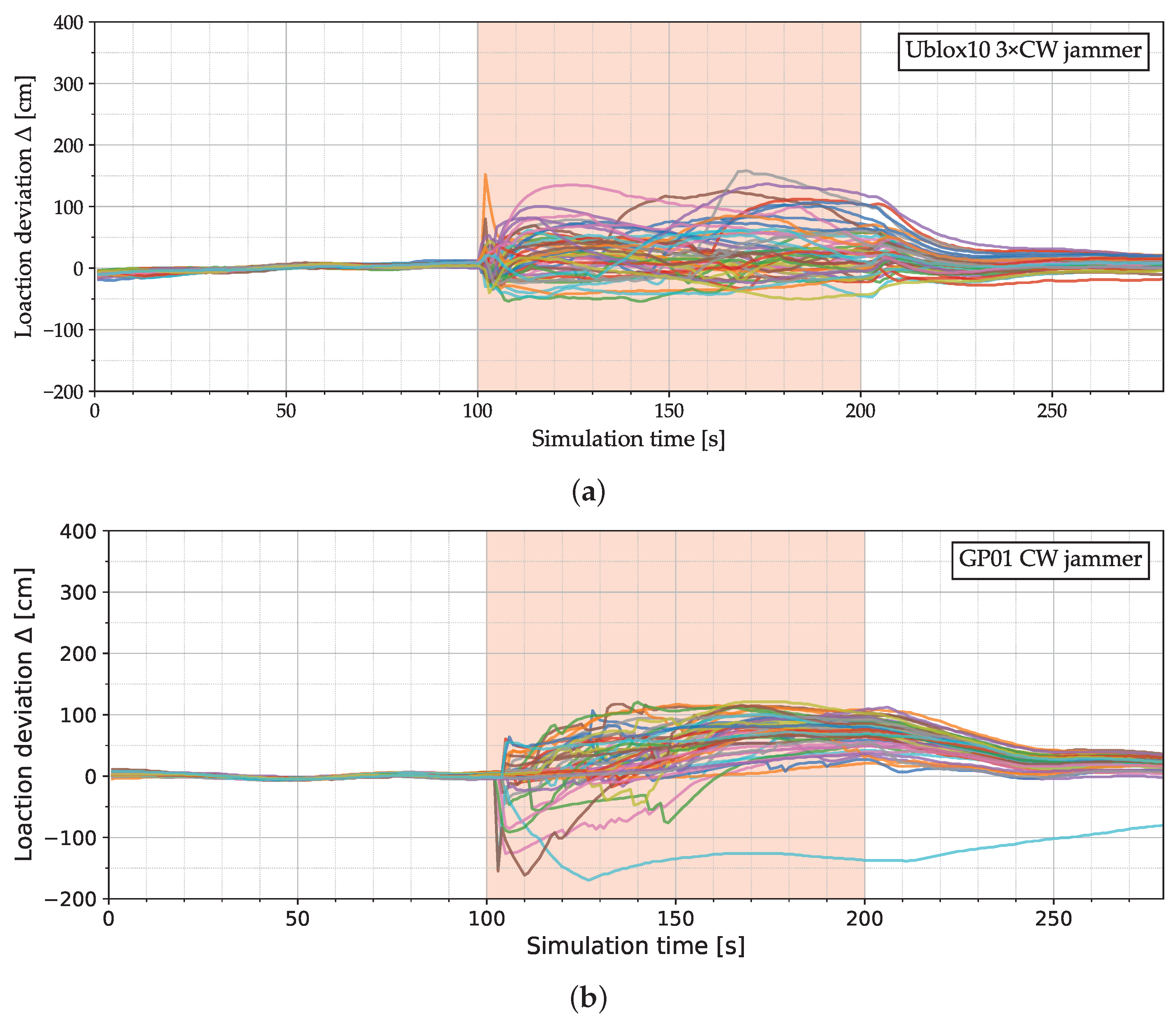
The positional deviation was calculated as the magnitude of the vector between the true position and the receiver’s reported position, representing the overall deviation without separate latitude and longitude components. A larger magnitude indicates a greater deviation from the reference. Positive values signify a north–east movement, and negative values a south–west movement from a true position. The graphs depict changes in centimeters relative to the initial stable state (the first 100 s) before any disturbances occurred, ensuring that all graphs start near Δ 0 cm. This effectively isolates the receiver’s dynamic response to disturbances by removing any fixed offset in the location’s center (as can be seen in Figure 3). Each of the 50 measurement repetitions is shown as a distinct colored curve, intentionally plotted together to highlight the complexity of interpreting the results and the substantial variability in the receiver’s behavior under jamming.

Figure 8a, a reference measurement without jamming, illustrates the baseline performance. As an older generation receiver (U-blox NEO-6M) relying solely on the GPS L1 signal, it exhibits minor positional fluctuations over time, but these remain within the expected 1 m accuracy range.

In stark contrast, the introduction of a broadband FM jamming signal, indicated by the red shaded area for 100 s, drastically alters the receiver’s behavior. Initially, the receiver shows minimal response to the relatively weak jamming. However, after 50 s, the effects become pronounced, manifesting as significant positioning errors. Notably, the severity of these errors varies considerably across repetitions. While some measurements show only moderate deviations over time, others exhibit substantial shifts, frequently exceeding 2 m and, in some instances, reaching 4 m. 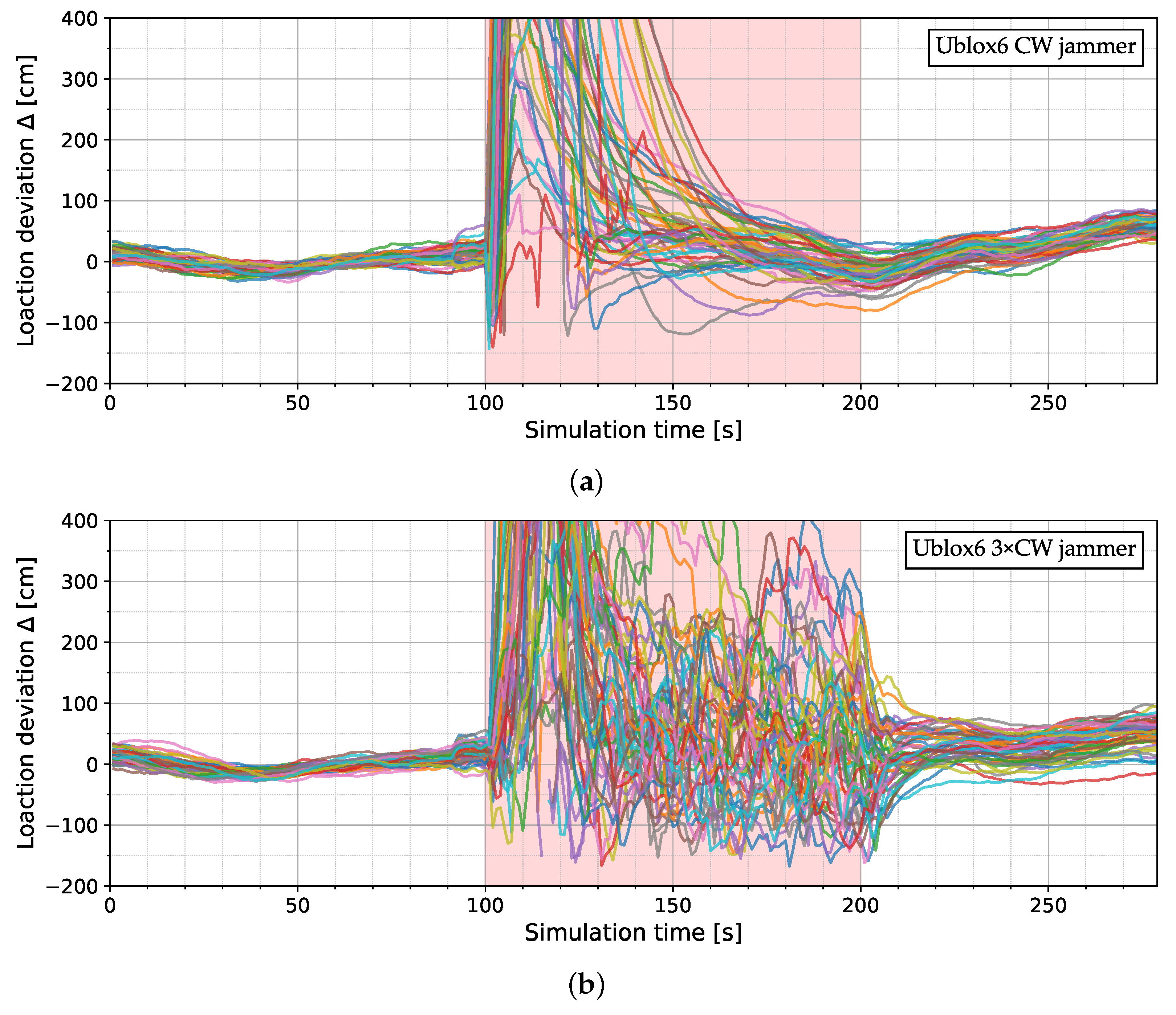Using the same receiver as in Figure 8, Figure 9 illustrates its response to single (a) and triple (b) CW interference at −70 dBm. With single-frequency interference, most repetitions show an immediate and substantial deviation from the true location, exceeding 10 m. The receiver’s internal mechanisms then work to mitigate the interference, gradually restoring positioning accuracy to within ±1 m. Triple-frequency interference, however, leads to a persistent inability to fully mitigate, resulting in continuous location fluctuations seen across all repetitions. While the errors diminish after the 100 s interference period, the receiver does not fully regain its initial location accuracy, a phenomenon more pronounced than in other interference modes.

As demonstrated in Figure 10, the U-blox 10-Series receiver showcases enhanced performance, in part due to its ability to receive signals from all four GNSS constellations (GPS, GLONASS, Galileo, BeiDou), unlike the GPS-only U-blox 6-Series (Figure 9a). This broader GNSS support, combined with internal adaptive notch filters and digitally adjustable gain amplifiers, enables effective mitigation of CW interference at −50 dBm, a level 20 dB higher (100 times more powerful) than the older generation could withstand. Despite an initial, brief accuracy loss, the position deviation remains largely within a 2 m radius, indicating robust performance under significantly stronger jamming. While evaluating individual measurement deviations over time offers some insight, it is challenging to identify overall response trends when faced with numerous curves.

Figure 8, Figure 9 and Figure 10 lack the clarity necessary to easily discern patterns in the GNSS receivers’ responses. In accordance with the statistically-driven assessment strategy proposed in this article, it is essential to process the raw measurements to reveal underlying trends. The most reliable approach identified during our measurements involved observing the median value across all repetitions and visualizing the standard deviation of the measurement set. The detailed implementation of this statistical analysis is provided in Appendix A. 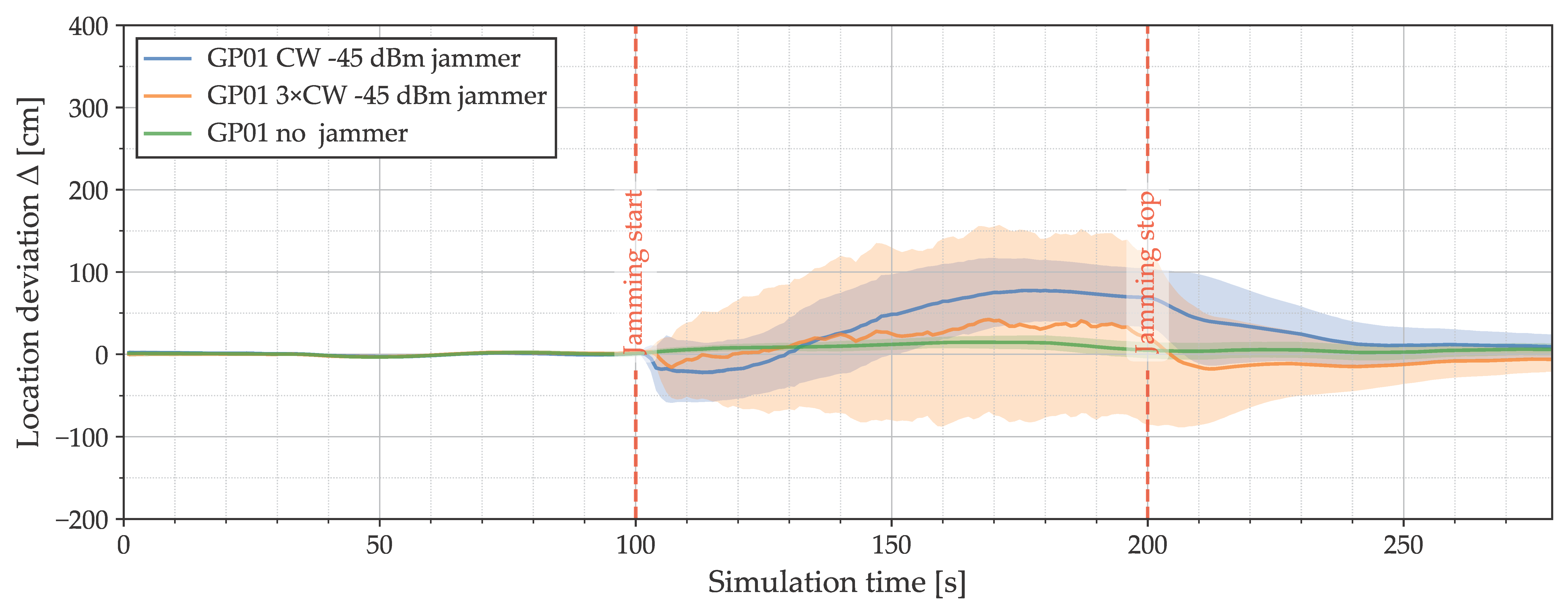Consequently, Figure 11 offers a significantly clearer perspective on the GP01 receiver’s response to a stronger jamming signal (−45 dBm) by displaying the median of all repeated measurements alongside their standard deviation. The shaded area around the median effectively represents the spread of individual measurements (which obscured patterns in the cluttered curves of earlier figures), with a wider area indicating greater variability between repetitions. The red vertical dashed lines indicate the interference period, and this consolidated view dramatically enhances readability compared to the previously cluttered plots.

As anticipated, the deviation remains minimal in the absence of interference (green curve), showing almost no increase over time. However, single-frequency (blue curve) and three-frequency (orange curve) CW jamming produce distinct patterns. Single-frequency interference results in a smaller position deviation, but the median deviates further away from the reference location. Conversely, three-frequency interference exhibits greater result dispersion (uncertainty), yet appropriate averaging allows for a closer approximation of the true position.

Figure 12 presents a compelling comparison of all three GNSS receivers studied in this research under three-frequency interference at equal power levels. Here, the GP01 receiver demonstrates superior performance, maintaining a median close to the true value despite a gradual increase in deviation over time. By contrast, the older U-blox 6-Series generation fails under such high interference levels. Its software is unable to mitigate the interference, leading to inaccurate location calculations. The receiver only regains its location fix after the interference ceases.

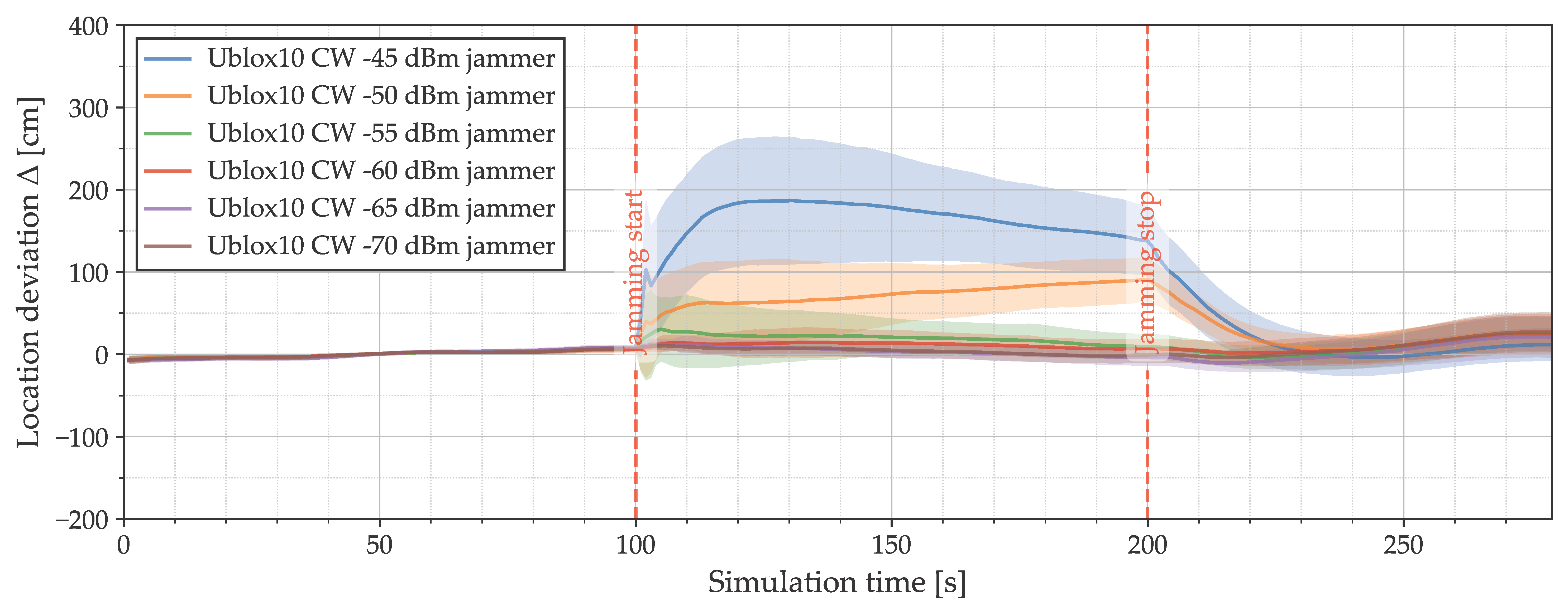
Lastly, Figure 13 addresses our core research question by illustrating receiver performance in a diverse jamming environment near its operational limits. Under these conditions, interference degrades position accuracy without a complete operational halt. Weak interference is depicted with a brown line, showing a negligible impact. By contrast, stronger interference (blue line) not only shifts the median location deviation across 50 repetitions but also introduces significant dispersion in the time series results of those repetitions. This highlights that a single measurement is insufficient for drawing conclusions about receiver response under jamming. As evidenced by the challenges in interpreting the cluttered charts of individual repetitions (like Figure 9b, indicating significant location determination problems reported by the receiver’s software under high interference), a thorough analysis using repeated measurements and appropriate visualization is crucial for truly understanding GNSS receiver behavior under jamming.

6. Discussion

A critical insight from our research is the significant and often overlooked unpredictability of GNSS receiver internal software in the context of jamming. Even when meticulous control over the input GNSS signal is achieved using calibrated sources in an attempt to isolate the receiver’s pure response, this software, as it actively tries to mitigate interference and maintain accurate fixes, introduces inconsistencies. Our GNSS simulator tests clearly demonstrate this, revealing varying responses to identical, repeated signal inputs. Consequently, traditional jamming impact assessments, often lacking in statistical depth, fail to capture the intricate temporal dynamics of receiver behavior, particularly under conditions that do not lead to immediate failure. To truly understand these effects, especially in less severe jamming scenarios, extensive measurement repetitions (around 50 in our study) coupled with statistical analysis (median and standard deviation) are essential. This necessity only intensifies under real-world conditions where constantly evolving satellite geometry, multipath, scattering, and diverse, prolonged jamming events introduce even greater variability, demanding a statistically sound approach for meaningful evaluation.

Our findings also reveal predictable trends: newer receiver generations, like the U-blox 10-series with its more sophisticated and evolved software, demonstrably handle interference far better than older models. This is evident in their ability to maintain near-full functionality even under stronger jamming levels compared to the U-blox 6-Series. Intriguingly, receiver responses still vary with interference type; for example, the 6th generation U-blox is highly susceptible to mid-L1 band CW signals but more tolerant of wider FM interference. Conversely, the multi-constellation U-blox 10th generation shows greater resilience to single-frequency CW, requiring substantially stronger interference to cause noticeable effects. While even the most advanced receivers will eventually fail under sufficiently strong interference, necessitating backup navigation, our results clearly indicate that utilizing newer generation multi-constellation and/or multi-frequency receivers offers significantly enhanced jamming mitigation capabilities compared to their predecessors. Although this work does not delve into specific mitigation strategies, the clear performance advantage of newer receivers like the U-blox 10 or Ai-Thinker GP-01 GP-01 underscores their importance in mitigating jamming effects.

So, how should the assessment of jamming responses in GNSS receivers be approached? The findings highlight the inherent uncertainty in these responses, advocating for a more systematic investigative approach. By initially focusing on the software response as the sole variable, a baseline for understanding receiver behavior can be established. Subsequent studies can then incrementally introduce real-world complexities like dynamic satellite constellations, ionospheric effects, and environmental factors. Furthermore, long-term field data collection, spanning weeks and employing multiple receivers with consistent antenna setups, is essential for comprehensive analysis.

Making the first steps in jamming assessment more accessible, we are publishing the extensive dataset generated during this research. This dataset, compiled over weeks using an automated laboratory setup, includes a multitude of receiver parameters (detailed in the linked public repository within the Data Availability Statement) and is provided as a valuable resource for the research community. The repository further offers a complete description of the data structure and illustrative examples for data manipulation, written in Python 3.13. Moreover, it contains the scripts used to generate the figures presented in this work. This comprehensive collection aims to showcase the dataset’s broad applicability and inspire further research utilizing this resource. Although this publication presents a focused analysis of the collected data, the full dataset unlocks a wide array of potential use cases, ranging from more granular response analysis and early jamming detection to the implementation of AI-driven time series algorithms for jamming mitigation.

Future investigations will expand to multi-frequency receivers and simulators, capturing more detailed receiver data, including spectrum observations and, importantly, capturing receiver responses under spoofing scenarios, similar to the dataset presented in this research. We are currently developing a receiver network for automated GNSS spectrum monitoring across a wide geographical area, with plans for long-term signal sampling at diverse locations. This will allow for the observation of region-specific variations in receiver behavior due to satellite visibility and elevation differences, contrasting with data from densely populated areas like Central Europe. Ultimately, laboratory-based interference response evaluations, as presented here, and the planned spoofing response analysis are vital for understanding and predicting receiver behavior in real-world scenarios.