A Mathematical Method of Current-Carrying Capacity for Shore Power Cables in Port Microgrids

Abstract

It is difficult to consider factors such as wind speed, water flow velocity, and solar radiation when using the IEC 60287 standard to calculate the current-carrying capacity of shore power cables in port microgrids. Therefore, based on the equivalent thermal circuit model and heat balance equation, this research takes solar radiation as the heat source of the cable used in port microgrids and proposes a mathematical calculation method for the current-carrying capacity of shore power cables based on the Newton–Raphson method. The influence of wind and water speed, environmental temperature, and solar radiation on current-carrying capacity is compared and analyzed using this mathematical calculation method and simulation calculation method. Shore power cables exhibit higher ampacity in water than air due to water’s superior thermal conductivity. Maximum ampacity difference occurs at 0.17 m/s flow (26.8 A analytically) and 0.066 m/s flow (64.4 A simulation). Air-laid cables show amplified ambient temperature effects from solar radiation, while water-laid cables demonstrate near-linear ampacity variations (Δ40 °C: 0–40 °C temperature range). This research can provide a reference for the revision of the standard for calculating the current-carrying capacity of shore power cables and optimizing renewable-energy-integrated port power systems.

1. Introduction

IEC 60287 [1] is a series of standards developed by the International Electrotechnical Commission (IEC) for the current rating, thermal performance, and loss calculation of power cables, aimed at regulating the safe operation and performance evaluation of cables under different environmental and load conditions. This standard provides a technical basis for cable design, manufacturing, laying, and operation through mathematical modeling and experimental verification, covering both AC and DC systems, and comprehensively considering factors such as laying methods, material characteristics, and environmental thermal conditions [2]. Central to its approach are assumptions about the thermal environment, including uniform soil thermal resistivity, stable ambient temperatures, and standardized burial conditions typical of land-based installations. While effective for conventional scenarios, these assumptions may not fully capture the complex thermal dynamics encountered in non-traditional settings, such as coastal environments. Shore power cables are key facilities connecting port microgrids with ships, and their increase in current-carrying capacity directly affects the power supply capacity and efficiency of microgrids. Shore power cables in port microgrids operate under markedly different conditions compared to standard land-based systems. These cables are integral to “cold ironing”, where ships docked at ports switch from onboard generators to grid-supplied electricity, reducing emissions. However, their installation environments often involves tidal zones or exposure to saltwater, which introduce unique thermal challenges. If the standard of IEC 60287 is adopted for calculating shore power cable’s current-carrying capacity, it is difficult to consider factors such as wind speed, water flow velocity, ambient temperature, and solar radiation on shore power cables in port microgrids.

Recently, the current-carrying capacity in shore power cables installed in port microgrids has been defined as the current flowing through the conductor when the temperature of the cable conductor reaches 90 °C, consequently requiring a calculation of temperature distribution [3,4]. As the calculation accuracy of the temperature field will directly affect the calculation accuracy of the cable current-carrying capacity, so the accurate calculation of the cable temperature field is the premise of the current-carrying capacity calculation. At present, the current-carrying capacity of cables is mainly obtained through experimental methods, analytical calculation methods, and numerical calculation methods. With the experimental method, it is difficult to simulate complex environmental conditions, and the construction and operation costs of the platform are high; analytical calculations have a certain degree of conservatism; numerical calculations can reflect environmental conditions in real time with high accuracy, but simulation model debugging is difficult, and the calculation cycle is long.

By measuring the surface temperature of cables using fiber optic sensors and combining it with the equivalent thermal path calculation method of cables, the conductor temperature of cables can be calculated [5]. Although this method is easy to calculate, there is still some error in calculating the conductor temperature from the surface temperature. At present, there are cables that use built-in optical fibers to directly measure the temperature of cable conductors, namely distributed optical fiber composite cables. This type of cable is manufactured by placing optical fibers along the inside of the cable [6,7]. Due to the high cost of laying distributed fiber optic cables along the route and their fragility, this type of distributed fiber optic composite cable is commonly used in submarine power transmission. As long as the temperature of the cable conductor is obtained, evaluation of the cable current-carrying capacity can be carried out. For some three-core cables, placing the optical fiber at the intersection of the three-phase conductor cores can accurately calculate the cable conductor temperature. Submarine cables typically place the optical unit inside a PET filler strip, outside the copper shielding tape or the inner sheath [6,8]. The use of a distributed built-in fiber optic temperature measurement not only enables real-time evaluation of the cable’s current-carrying capacity but also evaluates the degree of cable insulation degradation [9].

Currently, IEC standards and numerical calculations are typically used to calculate current-carrying capacity; however, the IEC standard’s calculation of current-carrying capacity is somewhat complex, with too many empirical formulas and correction coefficients, lacks a theoretical basis, makes it difficult to take complex external environment into consideration, and the calculation results are conservative [10]. The computation of the cable temperature distribution using the thermal circuit model was described in detail in [11]. In order to determine the cable’s carrying capacity, the numerical calculation approach can more accurately reflect the cable’s temperature distribution and simulate the real operating state of the cable as well as various external situations. The numerical calculation methods also include methods of finite differences, boundary elements, and finite elements [12], and the finite element approach works well for nonlinear, heterogeneous problems with complex geometric models [13]. There have been quite a lot of studies on using finite element simulation to calculate directly buried cables, trench cables, tubular cables, and tunnel cables; for reference, see [14,15,16,17]. The combination of an equivalent thermal circuit method to calculate the cable conductor temperature and a numerical method to calculate the field of soil temperature can effectively evaluate the cable current-carrying capacity [18,19]. In the literature [20], the conductor temperature is calculated by insulation layering based on the cable’s transient heat path. Research shows that the more the layering, the smaller the calculation error. In the literature [21], a dichotomous approach-based method was employed for calculating the cables’ current-carrying capacity. This method also analyzed how various factors affect this capacity, including soil thermal conductivity, ambient temperature, external heat sources, and the deep soil temperature. The literature [22] elaborated on the influence of soil water migration and closed air layer on the thermal path analytical model and proposed a method that integrates multi-physical numerical simulation with real-time environmental analysis to predict the real-time dynamic current-carrying capacity of power cables. In the literature [23], a method for calculating ampacity using the finite element method to study dynamic properties of thermal resistance is proposed, which can provide a reference for the analytical calculation method of IEC cable current-carrying capacity or modify the results. The method can also be extended to the estimation of parameters such as ambient temperature, buried depth of cable, and ventilation velocity. Cable current-carrying calculation using a multi-physics finite element method has also been applied to DC submarine cables [24].

Shore power cables in port microgrids have similarities and differences with land and sea cables; shore power cables are usually exposed to air but are sometimes submerged in water and can also be directly laid in water. The key to the calculation of the carrying capacity of shore power cables lies in the calculation of the temperature field. The calculation of the temperature field of a shore power cable in port microgrids not only needs to consider the heat production of the internal conductor of the cable but also needs to consider its special laying environment, such as the ambient temperature and the flow rate of the surrounding fluid, and also involves the physical characteristics of heat transfer, convection, and radiation. Therefore, the temperature distribution of shore power cables is studied by the method of electromagnetic-fluid-thermal-force coupling [25,26], and then the calculation method of ampacity in real time is studied.

This paper presents a mathematical model of the current-carrying capacity of shore power cables in port microgrids. Therefore, the impacts of wind speed, water flow velocity, ambient temperature, and solar radiation on the current-carrying capacity of shore power cables in port microgrids will be derived based on the equivalent thermal circuit model and heat balance equation. Then solar radiation is taken as the heat source of the cables, where it will be used to calculate of the current-carrying capacity of shore power cables. Considering the flow velocity and solar radiation, centered on solving surface temperature θ_s of shore power cables, so as to calculate the current-carrying capacity and the exterior thermal resistance T₄ of the cable, achieving the purpose of correcting the heat source and exterior thermal resistance T₄. The calculation of the exterior thermal resistance T₄ involves some empirical formulas, such as the heat dissipation coefficient h in T₄, which is the concentration of convective heat dissipation and radiative heat absorption. However, the IEC standard only provides a few typical laying methods of h calculation parameter values and does not strictly consider the impact of wind speed and water speed on shore power cables’ ampacity in port microgrids. This research addresses the disconnect between conventional IEC-based ampacity models and the dynamic thermal realities of port microgrids, which can provide a reference for the revision of the standard for calculating the ampacity of shore power cables and for the assessment of insulation ageing in port microgrids.

This article is organized into five sections. Section 1 explains the introduction and some of the previous works. Section 2 provides a short introduction of the shore power cable’s model, which includes a simulation and a physical model. Moreover, Section 2 explains the methodology for calculating the current-carrying capacity mathematically, based on a heat balance equation (HBE) using Newton–Raphson method. The results are in Section 3. Section 4 and Section 5 are conclusions and discussions.

2. Materials and Methods

2.1. Shore Power Cable Model

2.1.1. Simulation Model

In this research, we also use the electromagnetic-thermal-flow multi-physics simulation model of the shore power cable [27]. Figure 1 illustrates the construction of a 10 kV multi-physical field simulation model based on the installation of shore power lines in Foeryan Port, Chongqing, China. ANSYS 19.2 simulation software is used in the simulation. The two sections that make up the shore power cable-laying environment in this simulation are the air and the water.

2.1.2. Physical Model

The shore power cable CEU94-8.7/10 kV-3 × 120 mm² serves as the article’s research object. Figure 2 displays the cross-sectional structure, and constitutive material properties of the shore power cable are shown in

Table 1. Constitutive material properties of the shore power cable [27].

Parameter	Relative Dielectric Constant	Conductivity (S/m)	Specific Heat Capacity J/(kg·K)	Heat Conductivity W/(m·K)	Yang’s Modulus (GPa)	Poisson’s Ratio
Conductor	Tend to ∞	58 × 106	385	400	120	0.34
Insulation layer	3	Tends to 0	2300	0.2875	1.1	0.42
Conductor shied	100	6	1005	0.2875	1.7	0.41
Filler	1.6	Tends to 0	1883	0.0169	1.1	0.44
Inner sheath	3.6	Tends to 0	2100	0.2	0.64	0.41
Aluminum sheath	Tends to ∞	38 × 106	871	273	70	0.33
Outer sheath	3.5	Tends to 0	2070	0.2	0.2	0.42

.

2.2. Mathematical Algorithm for Ampacity Calculation of Shore Power Cable Using Heat Balance Equation

The heat balance equation refers to the transfer of heat between two or more systems with different temperatures until the temperature of the system is equal. In the process of heat exchange, it follows the laws of energy conversion and conservation.

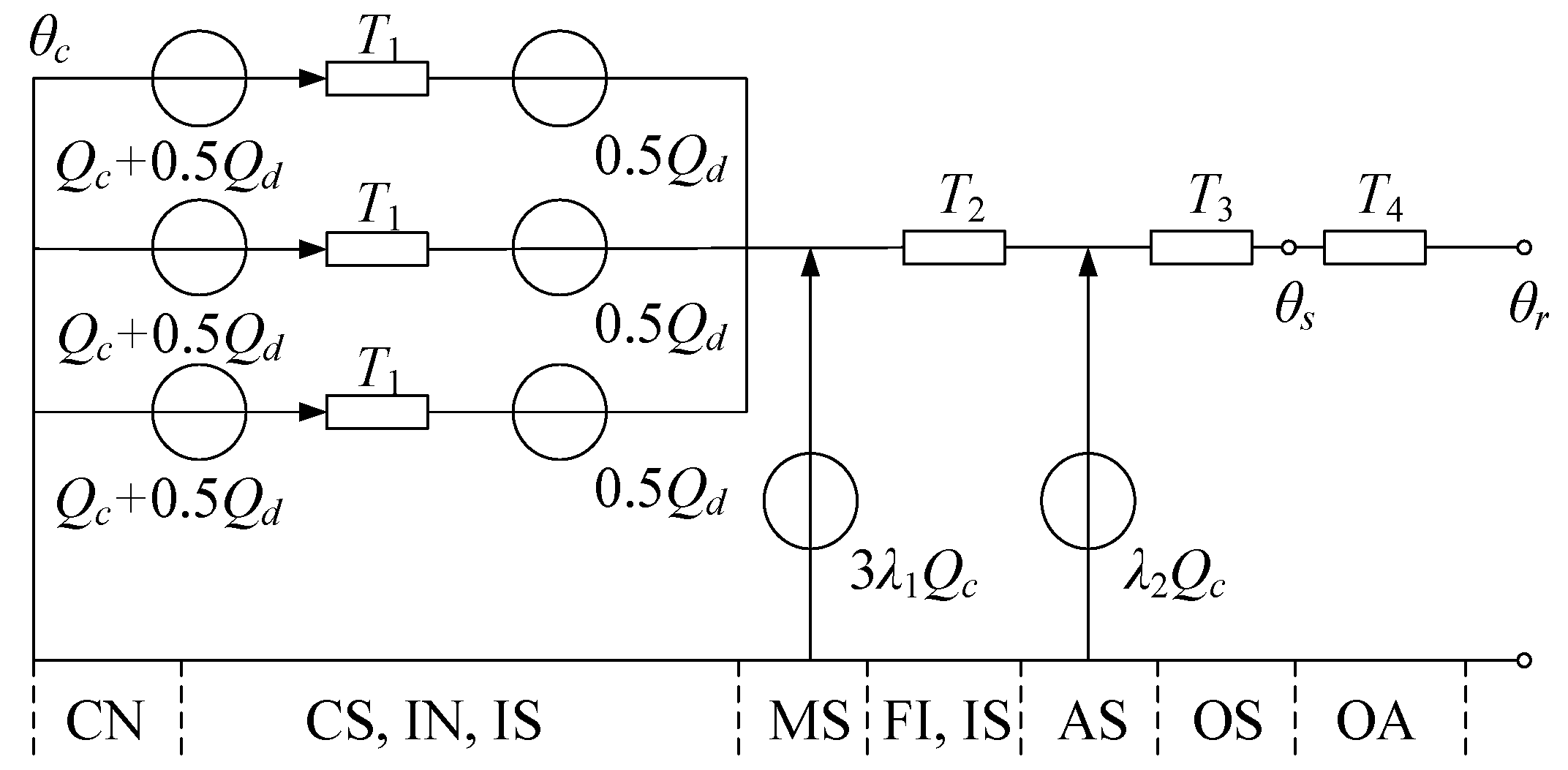
2.2.1. Thermal Circuit Model of Shore Power Cables

A thermal-circuit model provides an analogy between heat transfer phenomena and electrical circuit behavior, wherein thermal parameters are represented by corresponding electrical equivalents. In this conceptual framework, temperature differentials (ΔT) drive heat flux (Q) through thermal resistances, analogous to voltage potentials driving electrical current through resistors in Ohm’s law. This modeling approach enables the application of circuit analysis techniques—including series/parallel resistance combinations and nodal analysis—to solve complex heat transfer problems across composite materials and multi-domain thermal systems. The fundamental correspondence establishes temperature as the thermal potential, heat transfer rate as the thermal current, and material properties/geometric factors as thermal resistances, creating a powerful analytical tool for engineering thermodynamics.

Although the IEC 60287-prescribed ampacity determination method offers algorithmic simplicity and computational efficiency, the environmental dependence of the cable’s surface thermal resistance remains a critical parameter requiring careful consideration. This standard only provides some calculation methods for exterior thermal resistance under typical laying methods and is not universally applicable. Beginning with the shore power cable’s heat balance equation (HBE), the calculation technique may satisfy the requirements of calculating shore power cables’ ampacity by combining fluid mechanics and heat transfer theory. The equivalent thermal circuit approach specified in the IEC 60287 standard integrates the determination of exterior thermal resistance T₄, as depicted in the schematic diagram of Figure 3.

In Figure 3, Q_c is the conductor loss density (I²R per unit length), and Qd is the insulation and shielding loss density; the loss ratios λ₁ and λ₂ characterize the metallic shield and aluminum sheath losses relative to the total conductor losses. The thermal resistance network comprises the following: T₁ (insulation and shielding layers), T₂ (filling and inner sheath), T₃ (outer sheath), and T₄ (exterior thermal resistance).

According to Figure 3, the environmental temperature parameter can be determined through

$$\Delta \theta =(I^{2}R+0.5Q_d)T_1+[I^{2}R(1+{\lambda }_1)+Q_d]n{T}_2+[I^{2}R(1+{\lambda }_1+{\lambda }_2)+Q_d]n(T_3+T_4)$$

(1)

where I represents the conductor current; R denotes the alternating-current resistance per unit length; and n indicates the number of conductors. For the analyzed triple-core shore power cable system in this study, n = 3.

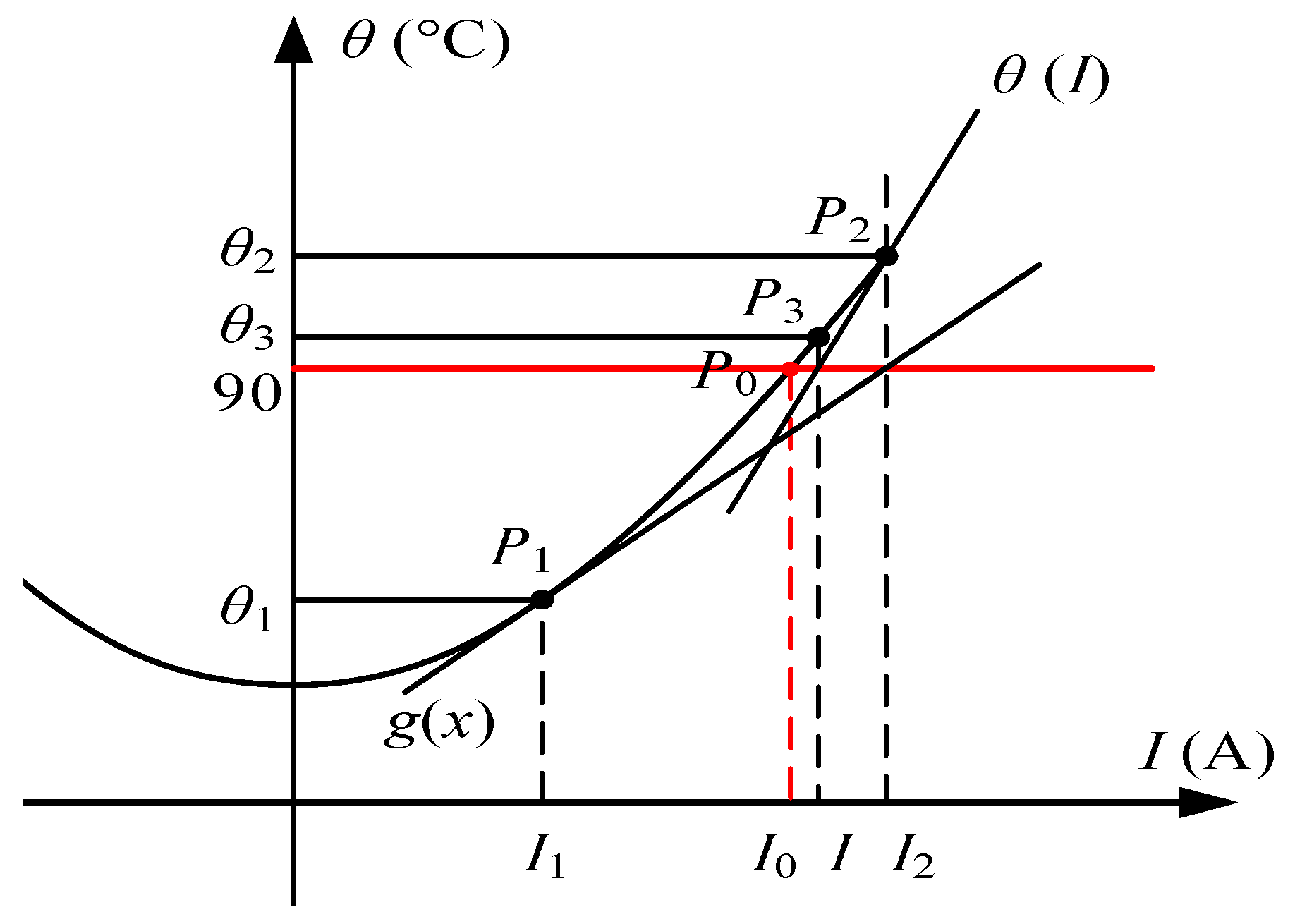
2.2.2. Newton–Raphson Method of Current-Carrying Capacity

Given the quadratic dependence of temperature on load current [4], the Newton–Raphson method is implemented for cable ampacity calculation, which based on the established functional relationship between peak insulation temperature and conductor current is

$$\mathit{\theta }\left(\mathit{I}\right)=\mathit{a}{\mathit{I}}^2+\mathit{f}({\mathit{e}}_1,{\mathit{e}}_2,{\mathit{e}}_3,\cdots ,{\mathit{e}}_{\mathit{n}})$$

(2)

where a is a system-specific constant that scales the quadratic term I², which represents the current parameter; $f(e_1,e_2,e_3,\cdots ,e_n)$ is a constant term of the $\theta \left(I\right)$ function, which is related to various environmental factors (temperature, humidity) and represented by variables $e_1$…$e_n$. The coefficient a and function f enable flexible modeling of both intrinsic nonlinearities (aI²) and extrinsic influences (f). Their definitions depend on the system’s physics, empirical data, or control objectives.

Figure 4 is a diagram of Newton–Raphson method. Let the straight line θ = 90 °C intersect with the curve $\theta \left(I\right)$ at point P₀; the value corresponding to P₀ is equal to I₀.

2.2.3. Heat Balance Equation (HBE) and Solution for Shore Power Cables

The thermal equilibrium characteristics of shore power cable systems are rigorously modeled through systematic application of the heat balance equation (HBE), incorporating both theoretical derivation and experimental validation methodologies. The cable surface temperature is determined using the Newton–Raphson method, where the total heat generation (comprising internal power losses and absorbed solar radiation) equals the combined convective and radiative heat transfer at the cable surface. The governing heat balance equation is expressed as follows:

$${\mathit{Q}}_{\mathit{i}}+{\mathit{Q}}_{\mathit{a}}={\mathit{Q}}_{\mathit{c}}+{\mathit{Q}}_{\mathit{r}}$$

(3)

where $Q_i$ represents the internal joule heating of the cable; $Q_a$ denotes the solar radiation absorption; and $Q_c$ and $Q_r$ correspond to the convective and radiative heat transfer components, respectively.

The function of cable surface temperature is

$$f\left({\theta }_s\right)=Q_r+Q_c-Q_a-Q_i$$

(4)

The derivative of the above Equation (4) with respect to θs is

$$f^{\prime }({\theta }_s)=C_0+C_1\cdot {\left({\theta }_s+273.15\right)}^3$$

(5)

In the equation, the coefficients [28] C₀ and C₁ are

$$\left\{\begin{array}{l}{C}_0=0.57\pi {N_{\mathrm{Re}}}^{0.485}\cdot {\lambda }_{air}\\ C_1=4\pi D_e{\xi }_{0}b\end{array}\right.$$

(6)

Reference [28] elaborates on the relationship between thermal radiation and temperature and derives the relationship between the derivative of heat flux and the third power of temperature.

The condition $\mathit{f}\left({\mathit{\theta }}_{\mathit{s}}\right)$ = 0 yields the cable surface temperature solution. This surface temperature enables the determination of the conductor, metallic shield, and aluminum sheath temperatures, thereby facilitating the calculation of the shore power cable’s ampacity.

The solution of Equation (4) still uses the Newton–Raphson method; the equation is

$${\theta }_s^{(n+1)}={\theta }_s^{\left(n\right)}-{\displaystyle \frac{f\left({\theta }_s^{\left(n\right)}\right)}{f^{\prime }\left({\theta }_s^{\left(n\right)}\right)}}$$

(7)

From the thermal circuit model of the cable, without considering the exterior thermal resistance T₄, taking the external surface temperature of the cable as the boundary and the radiated heat absorption as the heat generation term, the cable core temperature equation is derived as follows:

$$\begin{array}{ll}\hfill {\theta }_c(I)& =(I^{2}R+0.5Q_d+{\displaystyle \frac{Q_a}{n}})T_1+[I^{2}R(1+{\lambda }_1)+Q_d+{\displaystyle \frac{Q_a}{n}}]n{T}_2+\hfill \\ & [I^{2}R(1+{\lambda }_1+{\lambda }_2)+Q_d+{\displaystyle \frac{Q_a}{n}}]n{T}_3+{\theta }_s\hfill \end{array}$$

(8)

The derivative of the above equation with respect to the current is

$${{\theta }^{\prime }}_c(I)=2IR\left[T_1+(1+{\lambda }_1)n{T}_2+(1+{\lambda }_1+{\lambda }_2)n{T}_3\right]$$

(9)

The final iterative equation is solved as

$$I^{(n+1)}=I^{\left(n\right)}-{\displaystyle \frac{\theta \left(I^{\left(n\right)}\right)-90}{{\theta }^{\prime }\left(I^{\left(n\right)}\right)}}$$

(10)

2.3. Methodology of Mathematical Model for Current-Carrying Capacity

The methodologies of this work present the mathematical derivation of current-carrying capacity based on a heat balance equation (HBE) according to the thermal circuit model (IEC 60287). The thermal equivalent circuit model specified in IEC 60287 incorporates the computation of exterior thermal resistance T₄ as an essential component. Due to the fact that T₄ is calculated using empirical formulas, the conventional methodology faces significant challenges in satisfying the computational requirements for shore power cable ampacity under complex environmental conditions, which will lead to a decrease in the accuracy of the calculation results. Consequently, this study presents the explicit formulation of the cable’s heat balance equation (HBE), employs the Newton–Raphson method for surface temperature determination, and derives the cable’s current-carrying capacity from rigorous mathematical analysis.

Figure 5 illustrates the computational workflow for current-carrying capacity determination, with the procedural steps detailed as follows:

(1) Initialize the program. Initialize the surface temperature ${\theta }_s^{\left(0\right)}$ and current value $I^{\left(0\right)}$ of the cable, assign the monitored environmental factors to the variables, and set the conductor temperature constraints to θc = 90 °C;

(2) Calculate the conductor resistance R, determine the temperatures of both metallic shield and aluminum sheath, and calculate the loss factor, respectively. Then use Equation (8) to calculate the conductor temperature ${\theta }_c\left(I^{\left(0\right)}\right)$ and determine whether the difference between ${\theta }_c\left(I^{\left(0\right)}\right)$ and 90 satisfies the following equation:

$$\left|90-{\theta }_c\left(I^{\left(0\right)}\right)\right|\le {\epsilon }_1$$

(11)

If the convergence criterion is satisfied, the initial current value $I^{\left(0\right)}$ represents the cable’s ampacity. Otherwise, $I^{\left(1\right)}$ is calculated using Equation (10), and ${\theta }_c\left(I^{\left(1\right)}\right)$ is calculated by substituting Equation (8). Then, it is judged again whether Equation (11) is satisfied. If the convergence criterion is met, then $I^{\left(1\right)}$ is the ampacity. Otherwise, iteration is repeated until Equation (11) is satisfied, and the current-carrying capacity at surface temperature ${\theta }_s^{\left(0\right)}$ is obtained, denoted as $I^{(n, 0)}$;

(3) Calculate the values of Q_i, Q_a, Q_c, Q_r, and $f\left({\theta }_s^{\left(0\right)}\right)$ based on $I^{(n, 0)}$ and the cable temperature distribution as well as the external environment and check whether the following equation is satisfied:

$$f\left({\theta }_s^{\left(0\right)}\right)\le {\epsilon }_2$$

(12)

If the convergence criterion is met, then $I^{(n, 0)}$ is the ampacity. Otherwise, ${\theta }_s^{\left(1\right)}$ is calculated using Equation (7);

(4) Use steps (2)–(3) to recalculate the current-carrying capacity, denoted as $I^{(n, 1)}$, and judge whether $f\left({\theta }_s^{\left(1\right)}\right)$ satisfies Equation (12); if satisfied, then $I^{(n, 1)}$ is the ampacity. Otherwise, the iteration is repeated until Equation (12) is satisfied, and the final ampacity is $I^{(n, m)}$.

3. Results

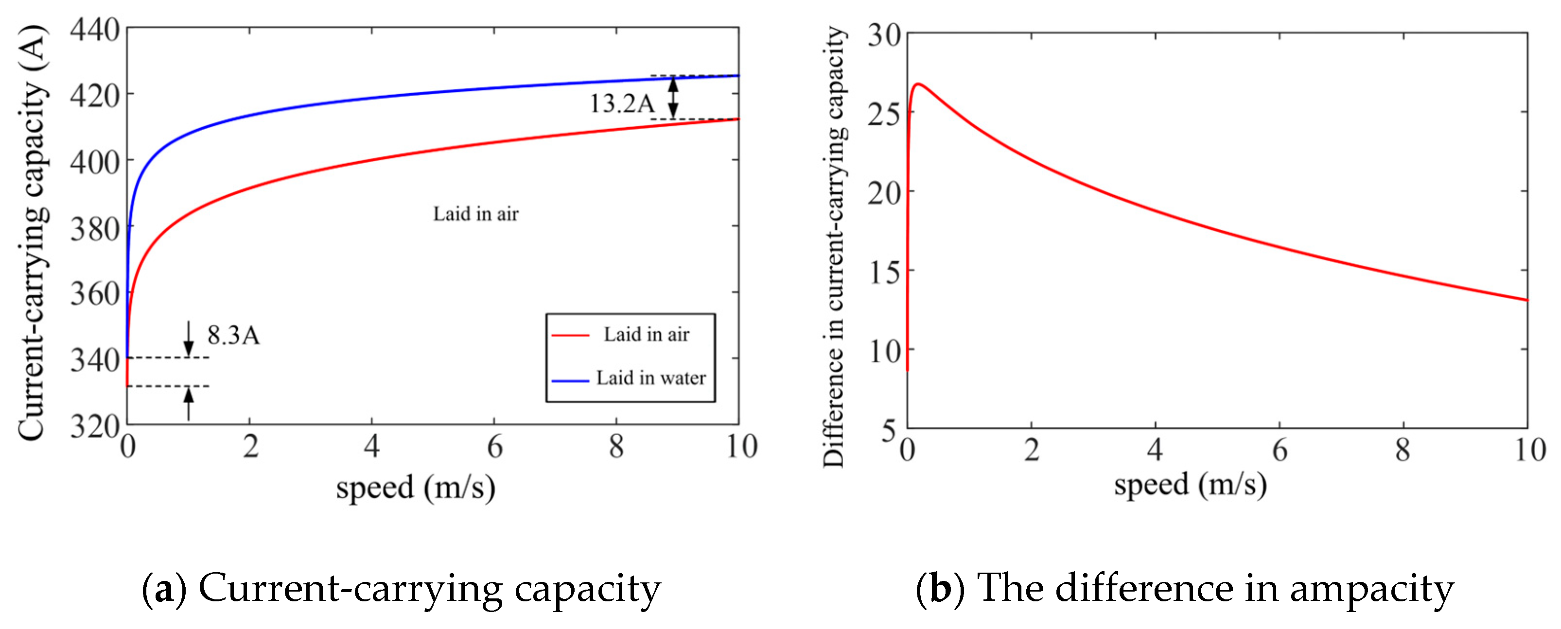
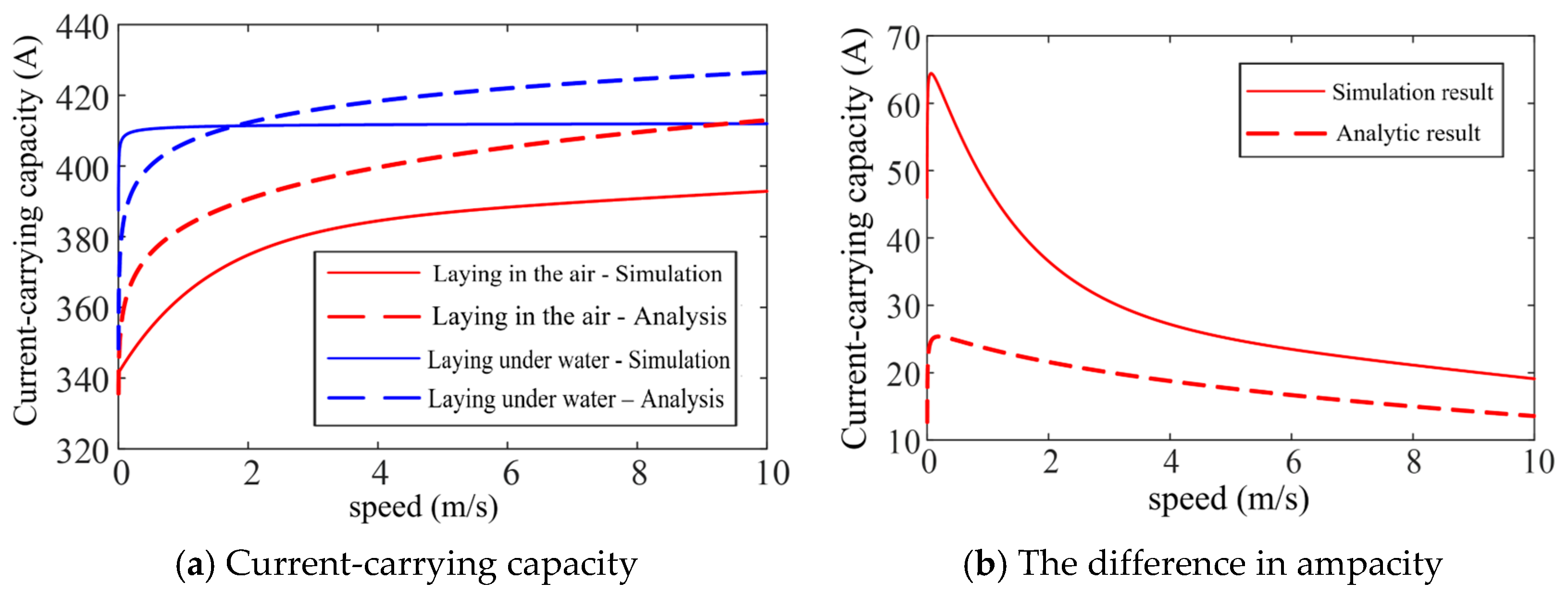
3.1. Influence of Wind and Water Speed

To integrate the effects of water and air speeds on the ampacity of shore power cables into a thermal model [29], the fluid flow velocities are typically incorporated through “convective heat transfer coefficients” in the heat balance equations. The cooling effect of wind or water flow on a cable is governed by “forced convection”. The heat dissipation from the cable surface depends on the convective heat transfer coefficient “h” [30], which is a function of fluid velocity, thermophysical properties (density, viscosity, thermal conductivity), and geometry. For air (wind), “hair” increases with wind speed due to enhanced airflow removing heat from the cable surface. For water, “hwater” is significantly higher than “hair” at the same velocity because water has higher thermal conductivity (kwater ≈ 0.6 W/m·K, kair ≈ 0.026 W/m·K) and heat capacity, leading to more efficient heat removal. In numerical simulations, when laying in the air, the wind speed increased from 0.001 m/s to 10 m/s, hair ≈ 5–250 W/m²K; when laying in water, the water flow velocity increased from 0.001 m/s to 10 m/s, and hwater ≈ 50–10,000 W/ m²K. For the same velocity, hwater ≫ hair, leading to higher ampacity in water as seen in Figure 6a.

Assuming that the shore power cable is laid in air and water, without considering the influence of solar radiation, and assuming that the solar radiation intensity H is zero and the environmental temperature is maintained at 20 °C, the influence of wind and water speed on the ampacity of shore power cables is analyzed, with results presented in Figure 6a. The cable’s current-carrying capacity exhibits a positive correlation with increasing speed; when laying in the air, the wind speed increased from 0.001 m/s to 10 m/s, and the ampacity of the shore power cable increased from 334.7 A to 409.9 A, an increase of 22.5%; when laying in water, the water flow velocity increased from 0.001 m/s to 10 m/s, and the ampacity of the shore power cable increased from 342.9 A to 423.2 A, an increase of 23.4%, but compared to air laying, it increased by 26.4%. Due to the better thermal conductivity of water compared to air, the ampacity of the shore power cable when laid in water is higher than when laid in air at the same flow rate. Figure 6b shows the variation curve of the difference of ampacity (ΔI) with wind speed and water flow velocity under the two laying methods. At 0.17 m/s, ΔI reaches its maximum, with a difference of 26.8 A.

3.2. Influence of Ambient Temperature

It is known from previous studies that the impact of environmental temperature on conductor temperature is approximately linear [27]. Does the ambient temperature demonstrate an approximately linear relationship with cable ampacity as well? The variation curve of the ampacity within the ambient temperature range [–20, 40] with the wind and water speed is numerically determined using an iterative computational algorithm, as shown in Figure 7. For example, when the ambient temperature θ_f is equal to zero, the current-carrying capacity I_max at wind velocities of 1 m/s and 10 m/s is 434.5 A and 464.1 A, respectively, with a difference of 29.6 A; under an ambient temperature of 40 °C, the maximum current-carrying capacities are determined to be 327.3 A and 347.1 A at wind velocities of 1 m/s and 10 m/s, respectively, with a difference of 19.8 A.

Figure 7 demonstrates that as the ambient temperature increases, the ampacity of the shore power cable gradually decreases, and the rate of decline increases, demonstrating an approximately linear relationship. In addition, the higher the ambient temperature, the slower the increase in current-carrying capacity with wind speed, as shown in Figure 8.

For comparative analysis with the IEC 60287-based analytical methodology, the analytical calculation and simulation calculation curves of current-carrying capacity at different flow rates are drawn, as shown in Figure 9, where the solid line represents simulation, the dashed line represents analysis, the red line represents laying in the air, and the blue line represents laying under water. When laying in the air, the simulated results are lower than the analytical results, and the error is small in the low wind speed region and slightly larger in the high wind speed region, but both are less than 10%. When laying under water, the simulated results in the low flow rate zone are higher than the analytical results, and the error is larger, while the simulated results in the high flow rate zone are lower than the analytical results, and the error is smaller, but both are less than 15%. For analytical calculation, when the flow rate is 0.17 m/s, the difference in ampacity between the two laying modes reaches the maximum, with a difference of 26.8 A. For simulation calculation, when the flow rate is 0.066 m/s, the difference in ampacity between the two laying modes reaches the maximum, with a difference of 64.4 A.

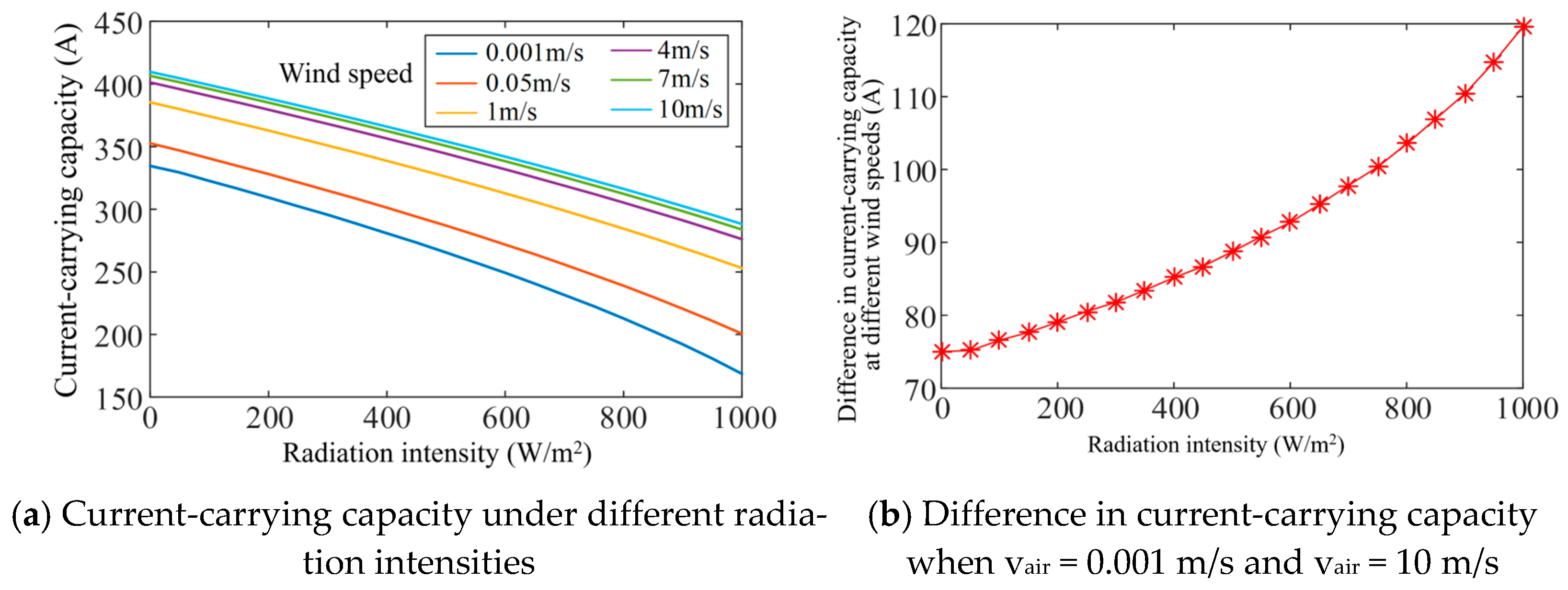
3.3. Effect of Solar Radiations

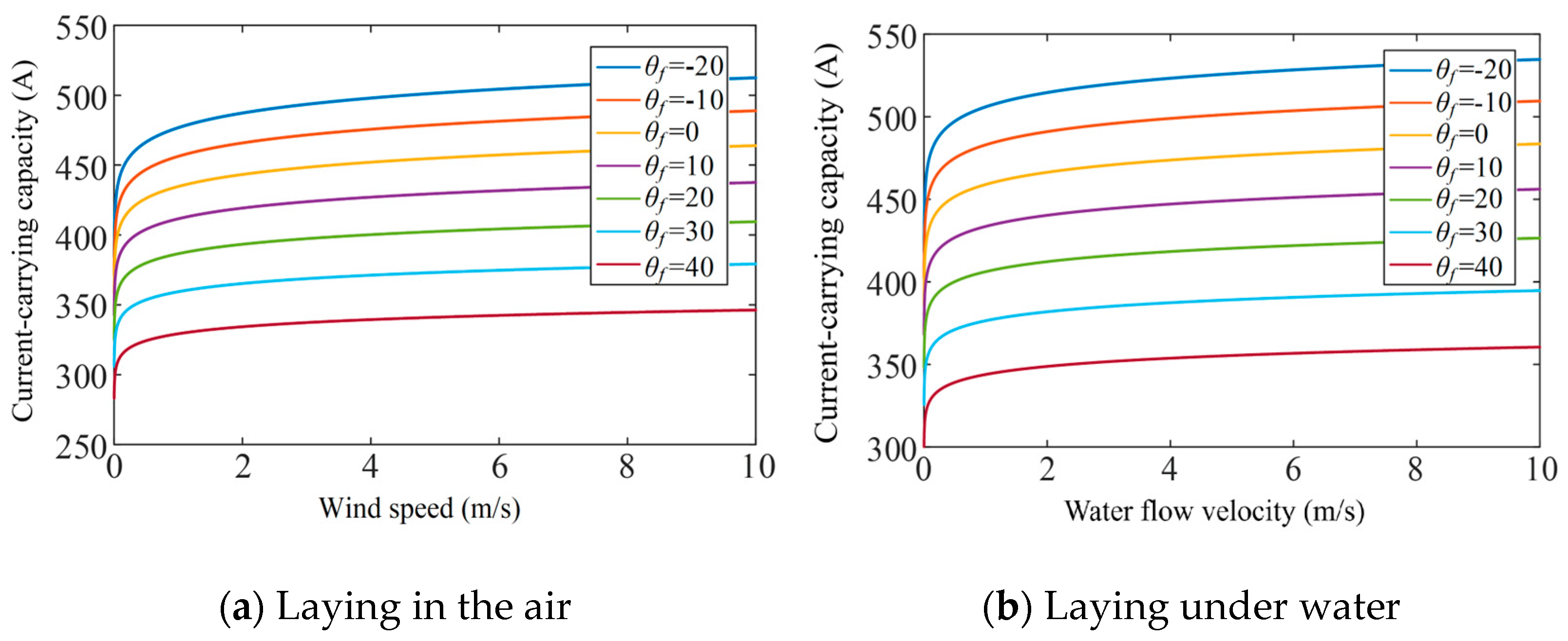
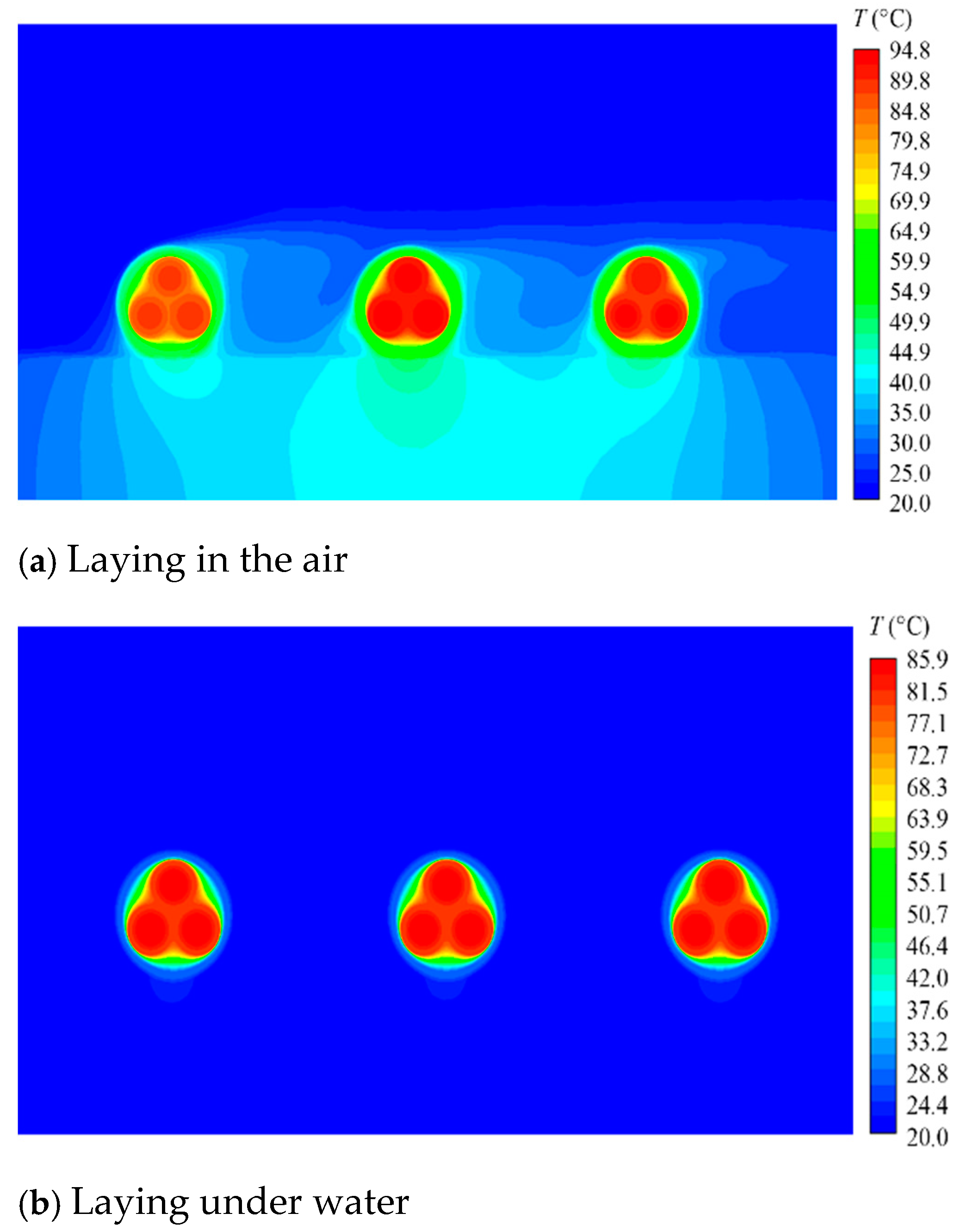
3.3.1. Laying in the Air

If there is solar radiation, the surface of the shore power cable will absorb a certain amount of radiant heat, and the temperature will further rise, causing a decrease in cable ampacity. When the shore power cable is laying in the air, considering an environmental temperature of 20 °C and a surface solar radiation absorption coefficient of 0.4, the range of solar radiation intensity is taken as [0, 1000], and the change rule of the ampacity of the shore power cable with solar radiation intensity under different wind speeds is calculated, as shown in Figure 10a. From the calculation results, it can be seen that as the radiation intensity increases, the ampacity of the shore power cable gradually decreases, and there is a nonlinear relationship between radiation intensity and current-carrying capacity. In addition, as the wind velocity increases, the linearity of the radiation intensity and the ampacity of the shore power cable improves, and the difference in ampacity at different speeds gradually increases, as shown in Figure 10b. When the radiation intensity H is 0, the current-carrying capacity at wind speeds of v_air = 0.001 m/s and 10 m/s is 334.6 A and 409.7 A, respectively, with a difference of 75.1 A; when the radiation intensity H = 1000 W/m², the current-carrying capacity at wind speeds v_air = 0.001 m/s and 10 m/s is 168.6 A and 288.2 A, respectively, with a difference of 119.6 A. That is to say, under constant ambient temperature conditions, the enhancing effect of wind speed on cable ampacity progressively intensifies with elevated solar radiation intensity, as quantitatively evidenced in

Table 2. Comparison of current-carrying capacity at v_air = 0.001 m/s and v_air = 10 m/s under different radiation intensities.

Radiation Intensity H (W/m2)	Wind Speed vair (m/s)		Current-Carrying Capacity Difference (A)
	0.001 m/s	10 m/s
0	334.6	409.7	75.1
200	309.4	388.5	79.1
400	280.8	366.0	85.2
600	249.2	342.0	92.8
800	212.7	316.3	103.6
1000	168.6	288.2	119.6

.

However, the ambient temperature also changes with the intensity of solar radiation, which directly determines the level of ambient temperature. With wind speed fixed at 1 m/s and solar radiation intensity varying within [0, 1000] W/m², the dependence of cable ampacity on solar radiation under different ambient temperatures is calculated and presented in Figure 11a. Numerical results demonstrate that reduced ambient temperatures enhance the linear correlation between solar radiation intensity and cable ampacity. Moreover, as the radiation intensity increases, the difference in current-carrying capacity at different temperatures gradually increases, as illustrated in Figure 11b.

When the radiation intensity H = 0, the current-carrying capacity at ambient temperatures T_r = 0 and T_r = 40 °C is 434.2 A and 328.0 A, respectively, with a difference of 106.2 A; when the radiation intensity H = 1000 W/m², the current-carrying capacity at ambient temperatures T_r = 0 and T_r = 40 °C is 322.6 A and 151.5 A, respectively, with a difference of 171.1 A. That is to say, under constant wind speed conditions, enhanced solar radiation intensity amplifies the impact of ambient temperature on shore power cable ampacity, with this temperature-dependent effect becoming progressively more pronounced as quantitatively demonstrated in

Table 3. Comparison of current-carrying capacity at T_r = 0 and T_r = 40 °C under different radiation intensities when laying in the air.

Radiation Intensity H (W/m2)	Ambient Temperature Tr ( °C)		Current-Carrying Capacity Difference (A)
	0 °C	40 °C
0	434.2	328.0	106.2
200	414.3	301.0	113.3
400	393.4	271.3	122.1
600	371.3	238.2	133.1
800	347.9	199.6	148.3
1000	322.6	151.5	171.1

.

In fact, ambient temperature not only exhibits dynamic variations in response to solar radiation intensity but also maintains intrinsic correlations with meteorological parameters. There exists a positive correlation between solar irradiance intensity and ambient temperature elevation. Therefore, the ampacity decreases faster with increasing solar radiation intensity, and its approximate relationship is similar to the black dashed line in Figure 11a.

3.3.2. Laying Under Water

If the shore power cable is laying under water, only part of the solar radiation reaches the cable’s external surface through the water surface because the water absorbs the solar radiation of a certain band. The transmission depends on the turbidity of the sea water and the immersion depth of the shore power cable. Turbidity levels exhibit a direct positive correlation with the degree of cloudiness in aqueous solutions, as quantified by nephelometric turbidity units.

As can be seen from Figure 12, when the laying depth is greater than 0.27 m, the ampacity of the shore power cables exhibits minimal variation with depth because the solar radiation energy is absorbed into the surface of the water, and minimal energy transfer occurs to the cable’s external surface. The ampacity of the shore power cable demonstrates a positive correlation with water turbidity levels because the solid particles in the water reflect part of the radiant energy back.

Assuming that the cable laying depth h = 0.5 m and the turbidity of water τ = 1 ntu, the impact of radiation intensity on ampacity calculated at different water velocities is shown in Figure 13a. When the radiation intensity H = 0, the current-carrying capacity at water velocities v_water = 0.001 m/s and v_water = 10 m/s is 342.9 A and 423.5 A, respectively, and the difference is 80.6 A. When the radiation intensity H = 1000 W/m², the current-carrying capacity at water velocities v_water = 0.001 m/s and v_water = 10 m/s is 309.2 A and 396.0 A, respectively, and the difference is 86.8 A. Figure 13b and

Table 4. Comparison of current-carrying capacity at v_water = 0.001 m/s and v_water = 10 m/s at different radiation intensities.

Radiation Intensity H (W/m2)	Water Flow Velocity vwater (m/s)		Current-Carrying Capacity Difference (A)
	0.001 m/s	10 m/s
0	342.9	423.5	80.6
200	336.6	418.1	81.5
400	330.1	412.7	82.6
600	323.2	407.2	84
800	316.2	401.6	85.4
1000	309.2	396.0	86.8

demonstrate that the ampacity difference between v_water = 0.001 m/s and v_water = 10 m/s exhibits an approximately linear increase.

When laying under water, the water temperature exhibits dependence on solar radiation intensity. Set water flow velocity as 1 m/s, cable laying depth h = 0.5 m, water turbidity τ = 1 ntu, and calculate the change rule of ampacity of the shore power cables with solar radiation intensity under different environmental temperatures, as illustrated in Figure 14a. The black dashed line is an approximate relationship drawn considering the impact of solar radiation on water temperature. When the radiation intensity H = 0, the current-carrying capacity at ambient temperatures T_r = 0 and T_r = 40 °C is 465.0 A and 348.0 A, respectively, with a difference of 117.0 A; when the radiation intensity H = 1000 W/m², the current-carrying capacity at ambient temperatures T_r = 0 and T_r = 40 °C is 440.3 A and 313.9 A, respectively, with a difference of 126.4 A. Figure 14b and

Table 5. Comparison of current-carrying capacity at T_r = 0 and T_r = 40 °C under different radiation intensities when laying under water.

Radiation Intensity H (W/m2)	Ambient Temperature Tr (°C)		Current-Carrying Capacity Difference (A)
	0 °C	40 °C
0	465.0	348.0	117.0
200	460.2	341.3	118.9
400	455.3	334.7	120.6
600	450.4	327.9	122.5
800	445.4	321.0	124.4
1000	440.3	313.9	126.4

show the difference in current-carrying capacity when T_r = 0 and T_r = 40 °C, which increases almost linearly.

In order to compare with the simulation, the water flow velocity was maintained at 1 m/s, the ambient temperature was set to 20 °C, the solar radiation intensity was 600 W/m², the load current for air laying was 313 A, and the load current for water laying was 394.4 A, with a laying depth of 0.5 m and a water turbidity of 1 ntu. The temperature distribution of the shore power cables for air laying and water laying was calculated through simulation, as shown in Figure 15. The air-laid conductor reaches a maximum temperature of 94.8 °C, exceeding the analytical prediction by 4 °C. The reason is that in the simulation calculation, the concrete will also be heated up by solar radiation; The maximum temperature for laying under water is 85.9 °C, which is 4.1 °C lower than the analytical calculation. This discrepancy may be attributed to the cable’s concrete interface, where the concrete structure is fully submerged in water, so its temperature distribution is almost unaffected by the shore power cable. As a whole, the shore power cable and concrete have a larger heat dissipation area, leading to a lower simulated temperature profile when compared with conventional analytical calculation.

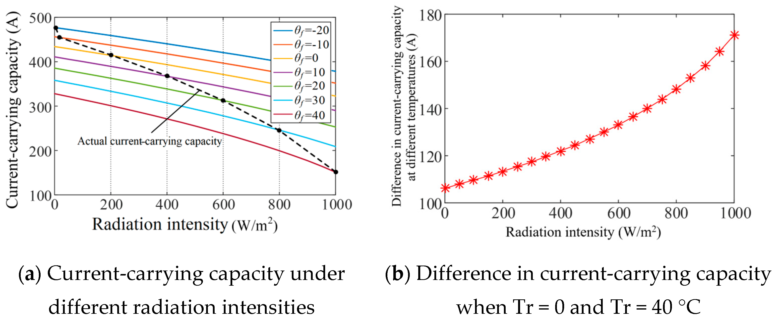
3.4. Influence of Exterior Thermal Resistance T₄

According to IEC 60287, the exterior thermal resistance T₄ quantifies the radial heat transfer characteristics per unit of cable length, serving as a critical parameter for evaluating cable-environment thermal interaction. Reduced T₄ values enhance heat dissipation, thereby increasing cable ampacity, while higher T₄ values restrict thermal transfer and decrease current-carrying capacity. In fact, the equivalent of this thermal resistance incorporates both convective and radiative heat transfer mechanisms at the cable surface. The IEC 60287 standard directly combines the two into a single coefficient T₄, making engineering calculations relatively simple but reducing accuracy.

3.4.1. Calculation of Exterior Thermal Resistance T₄ When Laying in the Air

The exterior thermal resistance coefficient T₄ exhibits functional dependence on both wind velocity and environmental temperature conditions.

Table 6. Thermal resistance coefficient T₄ at different wind speeds and ambient temperatures.

Ambient Temperature Tr (°C)	Wind Speed Vair (m/s)
	0.001	0.05	1	4	7	10
−20	0.813	0.580	0.268	0.158	0.125	0.107
−10	0.761	0.552	0.261	0.155	0.123	0.106
0	0.712	0.524	0.254	0.153	0.122	0.105
10	0.666	0.497	0.247	0.150	0.120	0.103
20	0.623	0.471	0.240	0.147	0.118	0.102
30	0.582	0.446	0.233	0.144	0.116	0.101
40	0.544	0.423	0.225	0.142	0.114	0.099

shows the thermal resistance coefficient T₄ at different wind velocities and environmental temperatures. The higher the wind velocity and environmental temperature, the smaller the exterior thermal resistance T₄, and the higher the wind velocity (such as 10 m/s), the less the thermal resistance coefficient (T₄) is affected by the ambient temperature.

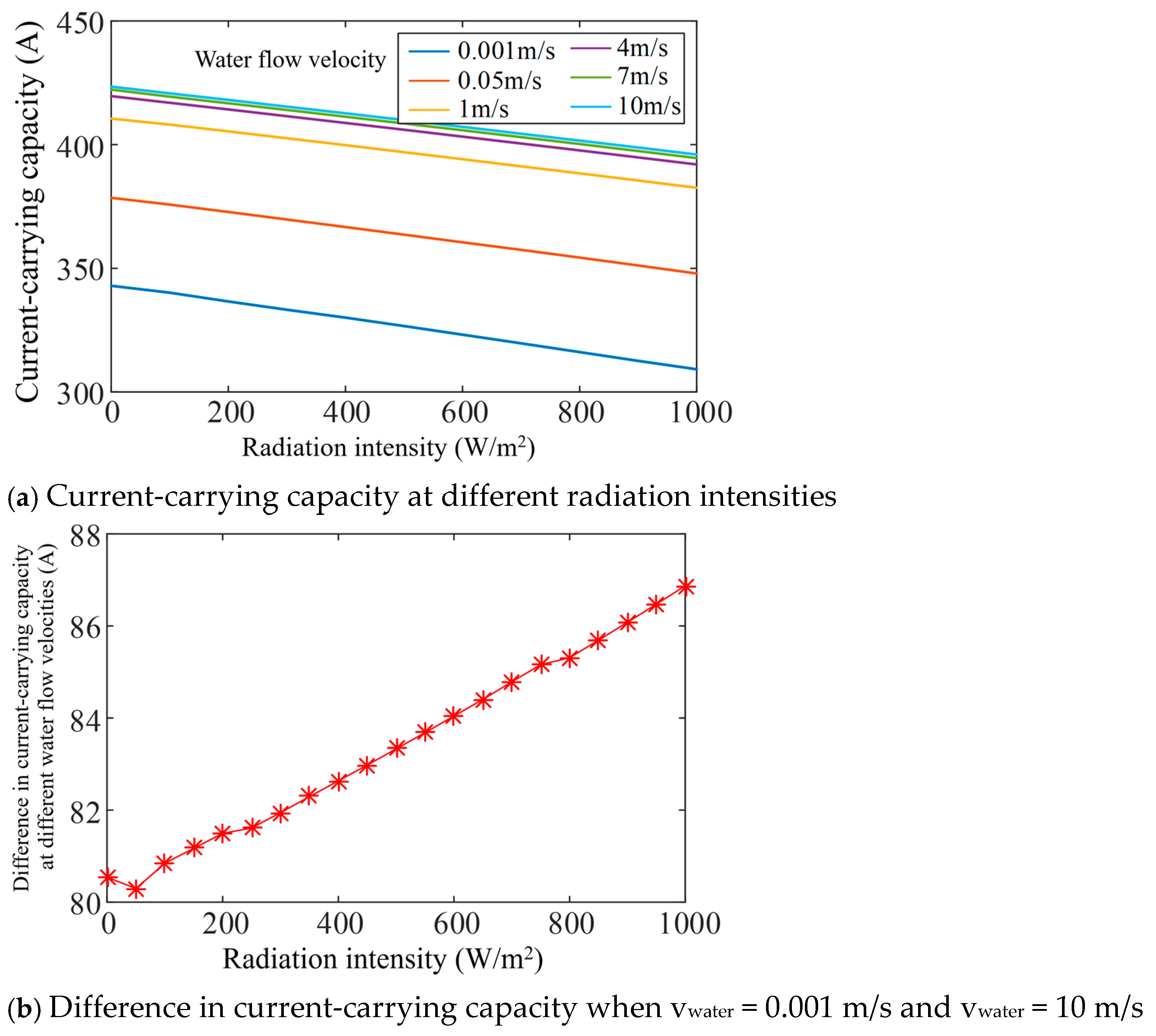
3.4.2. Calculation of Exterior Thermal Resistance T₄ When Laying Under Water

For submerged shore power cables, the thermal resistance coefficient T₄ remains functionally dependent on ambient temperature and water velocity. The thermal resistance coefficient T₄ calculated at different water flow velocities and ambient temperatures is shown in

Table 7. Thermal resistance coefficient T₄ at different ambient temperatures and water flow velocities.

Ambient Temperature Tr (°C)	Water Flow Velocity Vwater (m/s)
	0.001	0.05	1	4	7	10
−20	0.702	0.321	0.101	0.054	0.041	0.035
−10	0.662	0.312	0.099	0.053	0.041	0.035
0	0.623	0.302	0.098	0.053	0.041	0.035
10	0.587	0.292	0.097	0.053	0.041	0.035
20	0.552	0.283	0.096	0.052	0.041	0.035
30	0.519	0.273	0.095	0.052	0.040	0.034
40	0.488	0.263	0.094	0.052	0.040	0.034

. Its change rule is the same as that of laying in the air, but the heat dissipation performance of water is better than that of air, so the value of the thermal resistance T₄ is smaller than that of laying in the air. In addition, the thermal resistance T₄ is governed by the cable’s geometric surface characteristics (diameter-dependent) and radiative properties (material-dependent) of the outer sheath.

4. Conclusions

The ampacity of shore power cables is significantly influenced by environmental and operational factors, with wind/water speed, ambient temperature, solar radiation, and exterior thermal resistance (T₄) playing critical roles.

The existing IEC standards need to be upgraded from static models to dynamic environmental adaptability models, with a focus on the nonlinear effects of flow velocity, radiation, temperature gradient, and multi-factor coupling. Future research should combine intelligent monitoring and new material technology to promote the transformation of cable current-carrying capacity evaluation from “conservative design” to “precise dynamic regulation”, in order to meet the high reliability requirements of renewable energy grid connection and shore power systems.

5. Discussion

Due to the special application scenario of shore power cables, their current-carrying capacity is affected by wind and water velocity, ambient temperature, solar radiation, and exterior thermal resistance T₄.

It can be seen from the research that compared with the still state, the increase in wind and water velocity is significant for the ampacity of shore power cables, and a breeze of two to three knots can make the ampacity of the cable reach a relatively stable value. The flow velocity of water has the same effect, but the thermal conductivity of water is better than that of air, and the increase in ampacity is more significant. When laying under water, water has a certain absorption effect on solar radiation, and only part of the radiation is transmitted to the cable. The cable’s ampacity enhancement shows proportional improvement with increased burial depth and higher water turbidity levels, as these conditions reduce the amount of radiant energy reaching the cable’s surface. When laying in the air, solar radiation greatly reduces the ampacity of the shore power cable, so improvements can be made by reducing the absorption rate of solar radiation.

There are three measures to increase the ampacity of shore power cables in port microgrids:

(1) Optimize the cable’s surface properties by reducing its absorption coefficient while simultaneously enhancing emissivity and by using special materials, which can reflect electromagnetic waves in high radiation intensity bands;

(2) Optimize the laying method. The shore power cables utilized in port microgrids feature a lightweight design compared to conventional cables of equivalent voltage rating, enabling their installation through overhead suspension methods. This not only prevents direct solar radiation from shining on the cables and reduces the ampacity but also utilizes natural ventilation to increase the ampacity, increase the distance between cables when laying multiple circuits, and reduce the radiation heat transfer between each circuit;

(3) Adopt a hydrodynamic cooling approach. Shore power cables in port microgrids are generally short, and water cooling can be used if conditions permit, depending on the actual situation of the dock. For high-pile docks, shore power cables can be installed beneath the deck structure to mitigate temperature rise caused by solar exposure while leveraging the natural cooling effect of seawater or river water flow to enhance heat dissipation from the cables.

References

1. IEC 60287-1-1:2023; Electric Cables–Calculation of the Current Rating–Part 1-1: Current Rating Equations (100% Load Factor) and Calculation of Losses–General. International Electrotechnical Commission: Geneva, Switzerland, 2023.
2. Zeng, T.; Yang, G.; Yuan, M.; Chen, Y.; Fang, F.; Xu, X.; Lv, S.; Liu, G. Theoretical Modeling and Experimental Verification of AC Resistance in Large Cross-Section XLPE Single-Core Cables. In Proceedings of the 2024 The 9th International Conference on Power and Renewable Energy (ICPRE), Guangzhou, China, 20–23 September 2024; IEEE: New York, NY, USA, 2024. [Google Scholar]
3. Liu, Z.; Ouyang, B.; Liu, S.; Chu, F.; Li, T. Discussion on the Improvement of Current Carrying Capacity of AC 500 kV Submarine Cable. IOP Conf. Ser. Mater. Sci. Eng. 2019, 563, 052106. [Google Scholar] [CrossRef]
4. Zhang, L.; He, Y.; Liu, Y.; Yang, F.; He, T.; Liu, L.; Wang, S.; Liu, H. Temperature analysis based on multi-coupling field and ampacity optimization calculation of shore power cable considering tide effect. IEEE Access 2020, 8, 119785–119794. [Google Scholar] [CrossRef]
5. Chen, Y.; Wang, S.; Hao, Y.; Yao, K.; Li, H.; Jia, F.; Yue, D.; Shi, Q.; Cheng, Y.; Huang, X. Temperature Monitoring for 500 kV Oil-Filled Submarine Cable Based on BOTDA Distributed Optical Fiber Sensing Technology: Method and Application. IEEE Trans. Instrum. Meas. 2022, 71, 3504510. [Google Scholar] [CrossRef]
6. Yang, L.; Hu, Z.; Hao, Y.; Qiu, W.; Li, L. Internal temperature measurement and conductor temperature calculation of XLPE power cable based on optical fiber at different radial positions. Eng. Fail. Anal. 2021, 125, 105407. [Google Scholar] [CrossRef]
7. Cherukupalli, S.; Anders, G.J. Distributed Fiber Optic Sensing and Dynamic Rating of Power Cables; John Wiley & Sons: Hoboken, NJ, USA, 2019. [Google Scholar]
8. Zhang, Y.; Cen, Z.; Zhang, P.; Li, Q.; Hao, Y. Simulation Analysis of Burial Depth State of Optical Fiber Composite Submarine Cable Based on Temperature Field Variation. In Proceedings of the 2023 IEEE 4th International Conference on Electrical Materials and Power Equipment (ICEMPE), Shanghai, China, 7–10 May 2023; IEEE: New York, NY, USA, 2023; pp. 1–4. [Google Scholar]
9. Xu, Z.; Hu, Z.; Zhao, L.; Zhang, Y.; Yang, Z.; Hu, S.; Li, Y. Application of temperature field modeling in monitoring of optic-electric composite submarine cable with insulation degradation. Measurement 2019, 133, 479–494. [Google Scholar] [CrossRef]
10. Chen, X.; Yu, J.; Yu, L.; Zhou, H. Numerical analysis of thermo-electric field for AC XLPE cable in DC operation based on conduction current measurement. IEEE Access 2018, 7, 8226–8234. [Google Scholar] [CrossRef]
11. Henke, A.; Frei, S. Fast analytical approaches for the transient axial temperature distribution in single wire cables. IEEE Trans. Ind. Electron. 2021, 69, 4158–4166. [Google Scholar] [CrossRef]
12. Xiong, L.; Chen, Y.; Jiao, Y.; Wang, J.; Hu, X. Study on the effect of cable group laying mode on temperature field distribution and cable ampacity. Energies 2019, 12, 3397. [Google Scholar] [CrossRef]
13. Hadi, M.K. Utilization of the finite element method for the calculation and examination of underground power cable ampacity. Int. J. Appl. Power Eng. 2019, 8, 257–264. [Google Scholar] [CrossRef]
14. Zhang, Y.; Chen, X.; Zhang, H.; Liu, J.; Zhang, C.; Jiao, J. Analysis on the temperature field and the ampacity of XLPE submarine HV cable based on electro-thermal-flow multiphysics coupling simulation. Polymers 2020, 12, 952. [Google Scholar] [CrossRef] [PubMed]
15. Elsaid, A.M.; Zahran, M.S.; Abdel Moneim, S.A.; Lasheen, A.; Mohamed, I.G. A recent review on ventilation and cooling of underground high-voltage cable tunnels. J. Therm. Anal. Calorim. 2024, 149, 8927–8978. [Google Scholar] [CrossRef]
16. Che, C.; Yan, B.; Fu, C.; Li, G.; Qin, C.; Liu, L. Improvement of cable current carrying capacity using COMSOL software. Energy Rep. 2022, 8, 931–942. [Google Scholar] [CrossRef]
17. Wang, W.; Bai, X.; Si, W.; Zhao, Y.; Yao, W.; Liu, G.; Liu, H.; Yan, L.; Yang, D.; Meng, X.; et al. Review of Calculation Methods of Power Cables Temperature based on Thermal Circuit Model. In Proceedings of the 2024 IEEE 7th Advanced Information Technology, Electronic and Automation Control Conference (IAEAC), Chongqing, China, 15–17 March 2024; IEEE: New York, NY, USA, 2024; Volume 7, pp. 1711–1714. [Google Scholar]
18. Ma, A.; Zheng, M.; Zhang, S.; Qin, T. Thermal circuit model of DC submarine cable considering the influence of seawater property variations. Electr. Power Syst. Res. 2024, 230, 110268. [Google Scholar] [CrossRef]
19. Wang, X.W.; Zhao, J.P.; Zhang, Q.G.; Lv, B.; Chen, L.C.; Zhang, Y.; Yang, J.H. Real-time calculation of transient ampacity of trench laying cables based on the thermal circuit model and the temperature measurement. In Proceedings of the 2019 IEEE 8th International Conference on Advanced Power System Automation and Protection (APAP), Xi’an, China, 21–24 October 2019; IEEE: New York, NY, USA, 2019. [Google Scholar]
20. Wang, P.Y.; Ma, H.; Liu, G.; Han, Z.Z.; Guo, D.M.; Xu, T.; Kang, L.Y. Dynamic thermal analysis of high-voltage power cable insulation for cable dynamic thermal rating. IEEE Access 2019, 7, 56095–56106. [Google Scholar] [CrossRef]
21. Tang, J.; Fang, X.; Luo, X.; Qin, T.; Yang, T.; Ma, C.; Zhang, Y. Research on the Method of Improving the Current-carrying Capacity of Power Cable. J. Phys. Conf. Ser. 2022, 2247, 012042. [Google Scholar] [CrossRef]
22. Sun, D.; Dong, Q. Cable Steady-State Ampacity Correction Method based on Multi Physical Field Coupling Algorithm. Electroteh. Electron. Autom. 2022, 70, 19–27. [Google Scholar]
23. Zhang, H.; Ding, R.; Lin, P.; Zeng, Y.; Lyu, D.; Liu, G. Application of Thermal Resistance Dynamic Characteristics on High-Voltage Cable Ampacity Based on Field Circuit Coupling Method. In Proceedings of the 2022 12th International Conference on Power and Energy Systems (ICPES), Guangzhou, China, 23–25 December 2022; IEEE: New York, NY, USA, 2022; pp. 116–122. [Google Scholar]
24. Ge, J.; Wang, M.; Yang, Y.; Jing, Q.; Zhang, L.; He, J.; Zhou, Y.; Chang, Z.; Deng, J. Multi-Physics Simulation Study on Current Carrying Characteristics of High Voltage AC Submarine Cable Under Multiple Working Conditions. In Proceedings of the 2024 IEEE PES 16th Asia-Pacific Power and Energy Engineering Conference (APPEEC), Nanjing, China, 25–27 October 2024; pp. 1–5. [Google Scholar]
25. You, F.; Yusoh, M.A.T.M. A novel model to identify the performance of power cable on the offshore network by considering dynamic environmental impact. J. Phys. Conf. Ser. 2022, 2260, 012046. [Google Scholar] [CrossRef]
26. Tang, C.; Zhong, L.; Zeng, T.; Jiang, B.; Liu, D.; Cheng, R.; Yuan, C. Simulation and Analysis of Submarine Cable Based on Electro-Thermal-Flow Multi-physics Coupling. In Proceedings of the 2023 IEEE 4th International Conference on Electrical Materials and Power Equipment (ICEMPE), Shanghai, China, 7–10 May 2023; IEEE: New York, NY, USA, 2023; pp. 1–4. [Google Scholar]
27. You, F.; Yusoh, M.A.T.M.; Ali, N.H.B.N.; Yang, H. Analysis on Influencing Factors of Temperature Distribution of Shore Power Cable. IEEE Access 2024, 12, 137988–137999. [Google Scholar] [CrossRef]
28. Bergman, T.L. Fundamentals of Heat and Mass Transfer; John Wiley & Sons: Hoboken, NJ, USA, 2020. [Google Scholar]
29. Myklemyr, A. Analysis of Natural Convection and High Voltage AC Cable Rating in Naturally Ventilated Tunnels. Master’s Thesis, Norwegian University of Life Sciences, Ås, Norway, 2023. [Google Scholar]
30. Dehbani, M.; Rahimi, M.; Rahimi, Z. A review on convective heat transfer enhancement using ultrasound. Appl. Therm. Eng. 2022, 208, 118273. [Google Scholar] [CrossRef]
Figure 1. The simulation model of the shore power cable.
Electronics 14 01749 g001
Figure 2. A simplified 2D cross-sectional depiction of a shore power cable’s structure.
Electronics 14 01749 g002
Figure 3. Thermal network representation of 10 kV triple-core shore power cable system according to IEC 60287 standards.
Electronics 14 01749 g003
Figure 4. Diagram of Newton–Raphson method.
Electronics 14 01749 g004
Figure 5. The computational workflow for current-carrying capacity of shore power cables.
Electronics 14 01749 g005
Figure 6. Variation curve of ampacity of shore power cable with wind and water speed during air and water laying.
Electronics 14 01749 g006
Figure 7. Variation curve of ampacity of shore power cable with velocity at different ambient temperatures.
Electronics 14 01749 g007
Figure 8. Variation curve of ampacity of shore power cable with ambient temperature at different velocity.
Electronics 14 01749 g008
Figure 9. Comparison curve of simulation and analytical calculation of current-carrying capacity at different flow rates.
Electronics 14 01749 g009
Figure 10. Curve of current-carrying capacity under different radiation intensities and different wind speeds.
Electronics 14 01749 g010
Figure 11. Curve of current-carrying capacity under different radiation intensities and different temperatures when laying in the air.
Electronics 14 01749 g011
Figure 12. Impact of solar radiation on shore power cable ampacity when laying under water.
Electronics 14 01749 g012
Figure 13. Curve of current-carrying capacity at different radiation intensities and different water flow velocities.
Electronics 14 01749 g013
Figure 14. Curve of current-carrying capacity under different radiation intensities and different temperatures when laying under water.
Electronics 14 01749 g014
Figure 15. Temperature distribution at I = 313 A, V = 1 m/s, Tr = 20 °C, H = 600 W/m2.
Electronics 14 01749 g015