A k-Means Algorithm with Automatic Outlier Detection

Abstract

Data clustering is a fundamental machine learning task found in many real-world applications. However, real data usually contain noise or outliers. Handling outliers in a clustering algorithm can improve the clustering accuracy. In this paper, we propose a variant of the k-means algorithm to provide data clustering and outlier detection simultaneously. In the proposed algorithm, outlier detection is integrated with the clustering process and is achieved via a term added to the objective function of the k-means algorithm. The proposed algorithm generates two partition matrices: one provides cluster groups and the other can be used to detect outliers. We use both synthetic data and real data to demonstrate the effectiveness and efficiency of the proposed algorithm and show that the clustering performance of the proposed approach is better than other, similar methods.

1. Introduction

Data clustering or cluster analysis refers to the process of dividing a set of objects into groups or clusters such that objects in the same cluster are similar to each other and objects from different clusters are quite distinct [1,2,3]. Data clustering has found applications in a wide range of areas [4]. For example, data clustering is also used to sample insurance policies in order to build predictive models [5].

In the recent decades, many clustering algorithms have been developed by researchers from different fields [2,3,6]. Among these clustering algorithms, the k-means algorithm is one of the oldest and most commonly used clustering algorithms [7,8]. The k-means algorithm is also considered one of the top-ten algorithms in data mining [9]. Given a set of n data points $X=\{{\mathbf{x}}_1,{\mathbf{x}}_2,\dots ,{\mathbf{x}}_n\}$, the k-means algorithm tries to divide the dataset into k clusters by minimizing the following objective function:

$$P(U,Z)=\sum _{l=1}^k\sum _{i=1}^n{u}_{il}{\parallel {\mathbf{x}}_i-{\mathbf{z}}_l\parallel }^2,$$

(1)

where $U={\left(u_{il}\right)}_{n\times k}$ is an $n\times k$ partition matrix, $Z=\{{\mathbf{z}}_1,{\mathbf{z}}_2,\dots ,{\mathbf{z}}_k\}$ is a set of cluster centers, and $\parallel ·\parallel$ is the $L^2$ norm or Euclidean distance. The partition matrix U satisfies the following conditions

$$u_{il}\in \{0,1\},i=1,2,\dots ,n,l=1,2,\dots ,k,$$

(2)

$$\sum _{l=1}^k{u}_{il}=1,i=1,2,\dots ,n.$$

(3)

In the k-means algorithm, k is the desired number of clusters specified by the user. The optimization problem of minimizing (1) is NP-hard [10]. To minimize the objective function, the k-means algorithm starts from k initial cluster centers selected randomly from the dataset and then keeps updating the partition matrix U and updating the cluster centers Z alternately until some criterion is met.

One drawback of the k-means algorithm is that it does not have a built-in mechanism to detect outliers and its result is sensitive to outliers. Improving the k-means algorithm to handle outliers and noise data has the following benefits. First, considering outliers in the clustering process can improve the clustering accuracy of the k-means algorithm [11]. Second, outlier detection is an important data analysis task in its own right and has important applications in intrusion detection and fraud detection [12]. As a result, several clustering algorithms based on the k-means algorithm have been developed to handle outliers. See, for example, [11,12,13,14,15,16,17,18,19,20,21,22,23,24,25,26].

The existing clustering algorithms for handling outliers can be divided into two categories: multi-stage algorithms and single-stage algorithms. As its name indicates, a multi-stage algorithm performs clustering and detects outliers at multiple stages. Examples of multi-stage algorithms include [11,13,15,16,18,20]. The Outlier Removal Clustering (ORC) algorithm [11] is one of the earliest approaches proposed to enhance k-means by addressing the impact of outliers. Unlike multi-stage algorithms, single-stage algorithms integrate outlier detection into the clustering process. Examples of single-stage algorithms include [12,14,21,22,23,24,25,26,27].

Among the single-stage algorithms, the algorithms proposed in [14,27] are extensions of the fuzzy c-means algorithm. Others are variants of the well-known k-means algorithm. For example, the ODC (Outlier Detection and Clustering) algorithm [12], the NEO-k-means (non-exhaustive overlapping k-means) algorithm [22] and the k-means algorithm [21], and the KMOR (k-means clustering with outlier removal) algorithm [23] are extensions of the k-means algorithm that can provide data clustering and outlier detection simultaneously. A major difference between the KMOR algorithm and the other k-means variants (i.e., ODC, NEO-k-means and k-means) is that KMOR was based on the idea of an outlier cluster that was introduced by [28]. In KMOR, every data point in the outlier cluster has a constant distance from all data points. The constant distance is chosen to be the scaled average of the squared distances between all normal data points and their corresponding cluster centers.

However, one drawback of the KMOR algorithm is that it requires two parameters to control the number of outliers. Setting values for these parameters poses some challenges for real-world applications. In this paper, we propose the KMOD (k-means clustering with outlier detection) algorithm, which removes the drawback of the KMOR algorithm. In the proposed KMOD algorithm, the scaled average squared distance is incorporated into the objective function in an elegant way. There are two major differences between the KMOD algorithm and the KMOR algorithm:

• KMOD requires only one parameter to control the number of outliers, while KMOR requires two parameters to do this.
• In KMOD, outliers are used to update cluster centers with lower weights, while in KMOR, outliers are not used to update cluster centers.

Similarly to ODC, NEO-k-means, k-means--, and KMOR, the KMOD algorithm can also provide data clustering and outlier detection simultaneously.

The remaining part of this paper is organized as follows. In Section 2.1, we provide brief descriptions of some clustering algorithms that can conduct data clustering and outlier detection simultaneously. In Section 3, we present the KMOD algorithm in detail. In Section 4, we demonstrate the effectiveness of the KMOD algorithm using both synthetic data and real data. In Section 5, we conclude the paper with some remarks.

2. Related Work

In this section, we provide a review of the clustering methods that can detect outliers during the clustering process. In particular, we review the ODC algorithm, the NEO-k-means algorithm, the k-means-- algorithm, and the KMOR algorithm.

2.1. The ODC Algorithm

The ODC (Outlier Detection and Clustering) algorithm proposed by [12] is a modified version of the k-means algorithm. In the ODC algorithm, a data point that is at least $\gamma$ times the average distance from its centroid is considered an outlier. At each iteration, the average distance is calculated as follows:

$$d_{avg}={\displaystyle \frac{{\sum }_{l=1}^k{\sum }_{\mathbf{x}\in C_l}\parallel \mathbf{x}-{\mathbf{z}}_l\parallel }{k\left|X\right|}},$$

(4)

where k is the desired number of clusters, X is the dataset after outliers are removed, $\parallel ·\parallel$ is the Euclidean distance, and $\{{\mathbf{z}}_1,{\mathbf{z}}_2,\dots ,{\mathbf{z}}_k\}$ is a set of cluster centers.

Although the ODC algorithm is a modified version of the k-means algorithm, the ODC algorithm does not have an objective function that incorporates outliers explicitly. In fact, the ODC algorithm uses the following $SSE/SST$ ratio to measure the quality of the clustering results:

$${\displaystyle \frac{SSE}{SST}}={\displaystyle \frac{{\sum }_{l=1}^k{\sum }_{\mathbf{x}\in C_l}{\parallel \mathbf{x}-{\mathbf{z}}_l\parallel }^2}{{\sum }_{l=1}^k{\sum }_{\mathbf{x}\in C_l}{\parallel \mathbf{x}-\overline{\mathbf{x}}\parallel }^2}},$$

where $C_l$ is the lth cluster and $\overline{\mathbf{x}}$ is the mean of all the points in $C_1\cup C_2\cup \cdots \cup C_k$. For a fixed k, a lower value of the ratio indicates a better result. Note that data points that are considered as outliers are excluded from the calculation of $SSE/SST$.

In the ODC algorithm, outlier detection is not reversible in the sense that if a data point is considered an outlier at a particular iteration of the iterative process, then the data point cannot be changed back to be a normal point later.

2.2. The NEO-k-Means Algorithm

The NEO-k-means (non-exhaustive overlapping k-means) algorithm proposed by [22] can identify outliers during the clustering process. Its objective function is defined as

$$F(U,Z)=\sum _{j=1}^k\sum _{i=1}^n{u}_{ij}{\parallel {\mathbf{x}}_i-{\mathbf{z}}_j\parallel }^2,$$

(5)

where k is the desired number of clusters, $Z=\{{\mathbf{z}}_1,{\mathbf{z}}_2,\dots ,{\mathbf{z}}_k\}$ is a set of cluster centers, and $U={\left(u_{ij}\right)}_{n\times k}$ is a binary partition matrix. The matrix U satisfies the following conditions:

$$Tr\left(U^{T}U\right)=(1+\alpha )n,\sum _{i=1}^{n}I\left(\sum _{j=1}^k{u}_{ij}=0\right)\le \beta n.$$

where Tr(·) is the trace of a matrix and $I(·)$ is an indicator function.

In addition to the desired number of clusters k, NEO-k-means requires another two parameters: $\alpha$ and $\beta$. The parameter $\alpha$ controls the degree of overlap among clusters. The parameter $\beta$ controls the number of outliers. The maximum number of data points that can be considered outliers is $\beta n$. The objective function of the NEO-k-means algorithm is equivalent to that of the k-means algorithm when $\alpha =0$ and $\beta =0$.

The NEO-k-means algorithm minimizes the objective function iteratively. Given a fixed set of cluster centers, the algorithm first calculates the $nk$ distances between every data point and its center. Then, it updates the binary matrix U by assigning the first $n-\beta n$ data points to their closest centers. Then, it creates $\alpha n+\beta n$ more assignments by taking the $\alpha n+\beta n$ minimum distances from the $nk$ distances. Given the binary matrix, the algorithm updates the cluster centers to the means of the clusters. The above process is repeated until some stopping criterion is met.

2.3. The k-Means-- Algorithm

The k-means-- algorithm proposed by [21] provides data clustering and outlier detection simultaneously. The objective function of this algorithm is defined as

$$E(X,Z,L)=\sum _{\mathbf{x}\in X\setminus L}d{\left(\mathbf{x}\right|Z)}^2,$$

(6)

where X is the dataset, L is the set of outliers, Z is the set of cluster centers, and

$$d\left(\mathbf{x}\right|Z)=\underset{\mathbf{z}\in Z}{min}d(\mathbf{x},\mathbf{z}).$$

Here, $d(·,·)$ is a distance function. This algorithm requires two parameters, k and l, which specify the desired number of clusters and the desired number of top outliers, respectively.

In the k-means-- algorithm, an iterative procedure that is similar to k-means’ is used to minimize the objective function. In each iteration, the l top outliers are removed from the clusters before the cluster centers are updated. The l top outliers are defined to be the data points that have the l largest distances from their centers.

2.4. The KMOR Algorithm

Like the k-mean-- algorithm, the KMOR (k-means with outlier removal) algorithm proposed by [23] can also conduct data clustering and outlier detection simultaneously. Let k be the desired number of clusters. Motivated by the fuzzy clustering algorithm proposed by [27], the KMOR algorithm divides a dataset into $k+1$ groups, including k clusters and a group of outliers.

Mathematically, KMOR aims to minimize the following objective function:

$$P(U,Z)=\sum _{i=1}^n\left(\sum _{l=1}^k{u}_{il}{\parallel {\mathbf{x}}_i-{\mathbf{z}}_l\parallel }^2+\gamma u_{i,k+1}D(U,Z)\right)$$

(7)

subject to the following condition:

$$\sum _{i=1}^n{u}_{i,k+1}\le n_0,$$

where $0\le n_0<n$ and $\gamma \ge 0$ are parameters, $\parallel ·\parallel$ is the $L^2$ norm, $Z=\{{\mathbf{z}}_1$, ${\mathbf{z}}_2$, …, ${\mathbf{z}}_k\}$ is a set of cluster centers, and $U={\left(u_{il}\right)}_{n\times (k+1)}$ is a $n\times (k+1)$ binary partition matrix (i.e., $u_{il}\in \{0,1\}$) such that

$$\sum _{l=1}^{k+1}{u}_{il}=1,1\le i\le n,$$

and

$$D(U,Z)=\left({\displaystyle \frac{1}{n-{\sum }_{i=1}^n{u}_{i,k+1}}}\right)\sum _{l=1}^k\sum _{i=1}^n{u}_{i,l}{\parallel {\mathbf{x}}_i-{\mathbf{z}}_l\parallel }^2.$$

The two parameters $n_0$ and $\gamma$ work together to control the number of outliers. The maximum number of data points that can be considered outliers is $n_0$. When $\gamma =0$, then the number of outliers produced by the algorithm will be $n_0$. When $\gamma$ is large, then the number of outliers will be 0. As a result, the objective function of KMOR will be equivalent to that of k-means when $n_0=0$ or $\gamma \to \infty$.

The KMOR algorithm iteratively minimizes the objective function. Given a binary matrix U, the cluster centers are updated to be the means of the clusters. Given a set of cluster centers, the data points are assigned to clusters and the group of outliers as follows. If a data point’s distance to its center is greater than $\gamma D(U,Z)$, the point will be considered an outlier. If the number of such points is more than $n_0$, then the $n_0$ points that are furthest from their centers will be assigned to the group of outliers. If a data point’s distance to its center is not greater than $\gamma D(U,Z)$, then the data point will be assigned to its nearest cluster. This process is repeated until some stopping criterion is met.

3. The KMOD Algorithm

In this section, we present the KMOD (k-means with outlier detection) algorithm, which is an extension of the KMOR algorithm described in the previous section.

Let $X=\{{\mathbf{x}}_1,{\mathbf{x}}_2,\dots ,{\mathbf{x}}_n\}$ be a dataset containing n data points, each of which is described by d numerical attributes. Let k be the desired number of clusters. Let $U={\left(u_{il}\right)}_{n\times (k+1)}$ is a $n\times (k+1)$ binary partition matrix, such that

$$u_{il}\in \{0,1\},1\le i\le n,1\le l\le k+1,$$

(8)

$$\sum _{l=1}^{k+1}{u}_{il}=1,1\le i\le n.$$

(9)

The binary matrix U has $k+1$ columns. The last column of U is used to indicate whether a data point is an outlier; that is, $u_{i,k+1}=1$ if ${\mathbf{x}}_i$ is an outlier and $u_{i,k+1}=0$ if otherwise. If $u_{i,k+1}=0$, then $u_{il}=1$ for some $l\in \{1,2,\dots ,k\}$, where l is the index of the cluster to which ${\mathbf{x}}_i$ belongs. The binary matrix U divides the dataset X into $k+1$ groups, which include k clusters and one group of outliers.

Let $V={\left(v_{il}\right)}_{n\times k}$ is an $n\times k$ binary matrix such that

$$v_{il}\in \{0,1\},1\le i\le n,1\le l\le k,$$

(10)

$$\sum _{l=1}^k{v}_{il}=1,1\le i\le n.$$

(11)

Unlike U, the binary matrix V has k columns. The binary matrix V is a partition matrix that assigns all data points in X into the k clusters. If $v_{il}=1$, then the data point ${\mathbf{x}}_i$ is assigned to the lth cluster.

The objective function of the KMOD algorithm is defined as

$$\begin{array}{cc}\hfill & P(U,V,Z)\hfill \\ \hfill & =\sum _{i=1}^n\left(\sum _{l=1}^k{u}_{il}\parallel {\mathbf{x}}_i-{\mathbf{z}}_l{\parallel }^2+u_{i,k+1}{\displaystyle \frac{\gamma }{n}}\sum _{l=1}^k\sum _{j=1}^n{v}_{jl}{\parallel {\mathbf{x}}_j-{\mathbf{z}}_l\parallel }^2\right)\hfill \\ \hfill & =\sum _{i=1}^n\left(\sum _{l=1}^k{u}_{il}{\parallel {\mathbf{x}}_i-{\mathbf{z}}_l\parallel }^2+u_{i,k+1}D(V,Z)\right),\hfill \end{array}$$

(12)

where $\gamma \ge 0$ is a parameter, $Z=\{{\mathbf{z}}_1,{\mathbf{z}}_2,\dots ,{\mathbf{z}}_k\}$ is a set of cluster centers, $\parallel ·\parallel$ is the $L^2$ norm, and $D(V,Z)$ is the scaled average squared distance between all data points and their corresponding cluster centers, i.e.,

$$D(V,Z)={\displaystyle \frac{\gamma }{n}}\sum _{l=1}^k\sum _{j=1}^n{v}_{jl}{\parallel {\mathbf{x}}_j-{\mathbf{z}}_l\parallel }^2.$$

(13)

After some algebraic manipulation, we can write the objective function (12) as follows:

$$P(U,V,Z)=\sum _{i=1}^n\sum _{l=1}^k\left(u_{il}+v_{il}\gamma p_0\right){\parallel {\mathbf{x}}_i-{\mathbf{z}}_l\parallel }^2,$$

(14)

where

$$p_0={\displaystyle \frac{1}{n}}\sum _{j=1}^n{u}_{j,k+1},$$

that is, $p_0$ is the proportion of outliers. From Equation (14), we can see the following. If ${\mathbf{x}}_i$ is not an outlier, then $u_{il}=v_{il}=1$ for some $l\in \{1,2,\dots ,k\}$ and the contribution of ${\mathbf{x}}_i$ to the objective function is

$$(1+\gamma p_0){\parallel {\mathbf{x}}_i-{\mathbf{z}}_l\parallel }^2.$$

If ${\mathbf{x}}_i$ is an outlier, then $u_{il}=0$ for all $l=1,2,\dots ,k$ and $v_{il}=1$ for some $l\in \{1,2,\dots ,k\}$. In this case, the contribution of ${\mathbf{x}}_i$ to the objective function is

$$\gamma p_0{\parallel {\mathbf{x}}_i-{\mathbf{z}}_l\parallel }^2.$$

Thus, we can rewrite the objective function as

$$\begin{array}{cc}\hfill & P(U,V,Z)\hfill \\ \hfill & =\sum _{i\in I_N}(1+\gamma p_0)\parallel {\mathbf{x}}_i-{\mathbf{z}}_{m_i}{\parallel }^2+\sum _{i\in I_O}\gamma p_0{\parallel {\mathbf{x}}_i-{\mathbf{z}}_{m_i}\parallel }^2\hfill \\ \hfill & =\sum _{i\in I_N}\parallel {\mathbf{x}}_i-{\mathbf{z}}_{m_i}{\parallel }^2+\gamma p_0\sum _{i=1}^n{\parallel {\mathbf{x}}_i-{\mathbf{z}}_{m_i}\parallel }^2,\hfill \end{array}$$

(15)

where $m_i$ is the index of the center to which ${\mathbf{x}}_i$ is closest, and $I_N$ and $I_O$ are the index sets of normal points and outliers, respectively. From Equation (15), we can see that a point will be considered an outlier if the reduction in the first term is higher than the increase in the second term.

The goal of the KMOD algorithm is to find $U,V$, and Z, such that the objective function defined in Equation (12) is minimized. Like the k-means algorithm, the KMOD algorithm starts with a set of k initial cluster centers and then keeps updating U, V, and Z alternatively until some stopping criterion is met. The rules used to update U, V, and Z are summarized in the following three theorems.

Theorem 1.

Let $Z=Z^{🞶}$ and $U=U^{🞶}$ be fixed. If at least one data point is an outlier, i.e., $u_{i,k+1}^{🞶}=1$ for some i, then the binary matrix V that minimizes the objective function (12) is given as follows:

$$v_{jl}=\left\{\begin{array}{cc}1,\hfill & \mathit{if}\parallel {\mathbf{x}}_j-{\mathbf{z}}_l^{🞶}\parallel ={min}_{1\le s\le k}\parallel {\mathbf{x}}_j-{\mathbf{z}}_s^{🞶}\parallel ,\hfill \\ 0,\hfill & \mathit{otherwise},\hfill \end{array}\right.$$

(16)

for $j=1,2,\dots ,n$ and $l=1,2,\dots ,k$. If no data points are outliers, i.e., $u_{i,k+1}^{🞶}=0$ for all $i=1,2,\dots ,n$, then the objective function (12) is independent of V.

Proof. 

When $Z=Z^{🞶}$ and $U=U^{🞶}$, the objective function (12) becomes

$$\begin{array}{cc}\hfill & P(U^{🞶},V,Z^{🞶})=\hfill \\ \hfill & \sum _{i=1}^n\left(\sum _{l=1}^k{u}_{il}^{🞶}\parallel {\mathbf{x}}_i-{\mathbf{z}}_l^{🞶}{\parallel }^2+u_{i,k+1}^{🞶}{\displaystyle \frac{\gamma }{n}}\sum _{l=1}^k\sum _{j=1}^n{v}_{jl}{\parallel {\mathbf{x}}_j-{\mathbf{z}}_l^{🞶}\parallel }^2\right).\hfill \end{array}$$

If $u_{i,k+1}^{🞶}=0$ for all $i=1,2,\dots ,n$, then the objective function is independent of V. If $u_{i,k+1}^{🞶}=1$ for some i, then the objective function is minimized if the following function

$$D(V,Z^{🞶})={\displaystyle \frac{\gamma }{n}}\sum _{l=1}^k\sum _{j=1}^n{v}_{jl}{\parallel {\mathbf{x}}_j-{\mathbf{z}}_l^{🞶}\parallel }^2$$

is minimized. Since the rows of V are independent of each other, $D(V,Z^{🞶})$ is minimized if

$$\sum _{l=1}^k{v}_{jl}{\parallel {\mathbf{x}}_j-{\mathbf{z}}_l^{🞶}\parallel }^2$$

is minimized for all $j=1,2,\dots ,n$. Since $v_{jl}\in \{0,1\}$, the above equation is minimized if

$$v_{jl}=\left\{\begin{array}{cc}1,\hfill & \mathrm{if}\parallel {\mathbf{x}}_j-{\mathbf{z}}_l^{🞶}\parallel ={min}_{1\le s\le k}\parallel {\mathbf{x}}_j-{\mathbf{z}}_s^{🞶}\parallel ,\hfill \\ 0,\hfill & \mathrm{otherwise}.\hfill \end{array}\right.$$

This proves the theorem.    □

Theorem 2.

Let $V=V^{🞶}$ and $Z=Z^{🞶}$ be fixed. Then, the partition matrix U that minimizes the objective function (12) is established as follows:

$$u_{il}=\left\{\begin{array}{cc}1,\hfill & \mathit{if}\parallel {\mathbf{x}}_i-{\mathbf{z}}_l^{🞶}\parallel ={\eta }_i\hfill \\ 0,\hfill & \mathit{otherwise},\hfill \end{array}\right.$$

(17)

for $i=1,2,\dots ,n$ and $l=1,2,\dots ,k$, where

$${\eta }_i=min\left\{\parallel {\mathbf{x}}_i-{\mathbf{z}}_1^{🞶}\parallel ,\dots ,\parallel {\mathbf{x}}_i-{\mathbf{z}}_k^{🞶}\parallel ,\sqrt{D(V^{🞶},Z^{🞶})}\right\}.$$

For $l=k+1$, we have $u_{i,k+1}=1-{\sum }_{s=1}^k{u}_{is}$.

Proof. 

Since $V=V^{🞶}$ and $Z=Z^{🞶}$ are fixed and the rows of the partition matrix U are independent of each other, the objective function $P(U,V^{🞶},Z^{🞶})$ is minimized if, for each $i=1,2,\dots ,n$, the following function

$$\sum _{l=1}^k{u}_{il}{\parallel {\mathbf{x}}_i-{\mathbf{z}}_l\parallel }^2+u_{i,k+1}D(V^{🞶},Z^{🞶})$$

(18)

is minimized. Note that $u_{il}\in \{0,1\}$ for $l=1,2,\dots ,k+1$ and

$$\sum _{l=1}^{k+1}=1.$$

Equation (18) is minimized if

$$u_{il}=\left\{\begin{array}{cc}1,\hfill & \mathrm{if}\parallel {\mathbf{x}}_i-{\mathbf{z}}_l^{🞶}\parallel ={\eta }_i\hfill \\ 0,\hfill & \mathrm{otherwise},\hfill \end{array}\right.$$

for $l=1,2,\dots ,k$. This completes the proof.    □

Theorem 3.

Let $U=U^{🞶}$ and $V=V^{🞶}$ be fixed. Then, the cluster centers Z that minimize the objective function (12) are derived as follows:

$$\begin{array}{ccc}\hfill z_{ls}& =& {\displaystyle \frac{{\sum }_{i=1}^n{u}_{il}^{🞶}{x}_{is}+{\sum }_{i=1}^n{u}_{i,k+1}^{🞶}\frac{\gamma }{n}{\sum }_{j=1}^n{v}_{jl}^{🞶}{x}_{js}}{{\sum }_{i=1}^n{u}_{il}^{🞶}+{\sum }_{i=1}^n{u}_{i,k+1}^{🞶}\frac{\gamma }{n}{\sum }_{j=1}^n{v}_{jl}^{🞶}}}\hfill \\ & =& {\displaystyle \frac{{\sum }_{j=1}^n\left(u_{jl}^{🞶}+v_{jl}^{🞶}\frac{\gamma }{n}{\sum }_{i=1}^n{u}_{i,k+1}^{🞶}\right)x_{js}}{{\sum }_{j=1}^n\left(u_{jl}^{🞶}+v_{jl}^{🞶}\frac{\gamma }{n}{\sum }_{i=1}^n{u}_{i,k+1}^{🞶}\right)}}\hfill \end{array}$$

(19)

for $l=1,2,\dots ,k$ and $s=1,2,\dots ,d$.

Proof. 

When $V=V^{🞶}$ and $U=U^{🞶}$, the objective function (12) becomes

$$\begin{array}{cc}\hfill & P(U^{🞶},V^{🞶},Z)=\hfill \\ \hfill & \sum _{i=1}^n\left(\sum _{l=1}^k{u}_{il}^{🞶}\parallel {\mathbf{x}}_i-{\mathbf{z}}_l{\parallel }^2+u_{i,k+1}^{🞶}{\displaystyle \frac{\gamma }{n}}\sum _{l=1}^k\sum _{j=1}^n{v}_{jl}^{🞶}{\parallel {\mathbf{x}}_j-{\mathbf{z}}_l\parallel }^2\right).\hfill \end{array}$$

The above equation is minimized if its derivative with respect to $z_{ls}$ is equal to zero for all $l=1,2,\dots ,k$ and $s=1,2,\dots ,d$; that is,

$$\begin{array}{cc}\hfill & {\displaystyle \frac{\mathsf{\partial }P}{\mathsf{\partial }{z}_{ls}}}=\hfill \\ \hfill & \sum _{i=1}^n\left[-2u_{il}^{🞶}(x_{is}-z_{ls})-2u_{i,k+1}^{🞶}{\displaystyle \frac{\gamma }{n}}\sum _{j=1}^n{v}_{jl}^{🞶}(x_{js}-z_{ls})\right]=0,\hfill \end{array}$$

which leads to Equation (19). This completes the proof.    □

Note that we can also use Equation (14) to prove Theorem 3 and we can write Equation (19) as follows:

$$z_{ls}={\displaystyle \frac{{\sum }_{j=1}^n\left(u_{jl}^{🞶}+v_{jl}^{🞶}\gamma p_0\right)x_{js}}{{\sum }_{j=1}^n\left(u_{jl}^{🞶}+v_{jl}^{🞶}\gamma p_0\right)}},$$

where $p_0$ is the proportion of outliers found in the dataset. From the above equation, we see that the center of a cluster is calculated as the weighted average of the data points that are closest to the center of the cluster. However, a normal point has a weight of $1+\gamma p_0$ and an outlier is given a weight of $\gamma p_0$. Thus, the impact of outliers on cluster centers is also reduced in the KMOD algorithm.

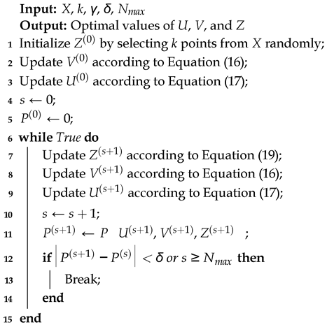
The pseudo-code of the KMOD algorithm is shown in Algorithm 1. The KMOD algorithm requires four parameters: k, $\gamma$, $\delta$, and $N_{max}$. Parameter k is the desired number of clusters for a particular dataset. Parameter $\gamma$ is a positive real number used to control the number of outliers. In general, a smaller value for $\gamma$ will result in more outliers. If $\gamma$ is close to zero, then all data points will be assigned to the outlier group. The last two parameters, $\delta$ and $N_{max}$, are used to terminate the iterative process. Some default values of $\gamma$, $\delta$, and $N_{max}$ are shown in

Table 1. Default values for some parameters required by the KMOD algorithm.

Parameter	Default Value
$\gamma$	2
$\delta$	${10}^{-6}$
$N_{max}$	100

.

The difference between KMOD and KMOR is that the former uses outliers with low weights to update the cluster centers but the latter does not use outliers to update centers. In addition, KMOD does not require users to set a maximum number of outliers. Instead, the number of outliers is controlled by parameter $\gamma$.

Algorithm 1: The KMOD Algorithm

4. Numerical Experiments

In this section, we conduct numerical experiments based on both synthetic data and real data to show the effectiveness of the KMOD algorithm. All algorithms were implemented in Java and the source code is available at https://github.com/ganml/jclust, accessed on 21 April 2025.

4.1. Validation Measures

In our experiments, we used the following validation measures to measure the accuracy of the clustering results: the adjusted Rand index (ARI) [29], the normalized mutual information (NMI) [30], and the classifier distance [12]. The first two measures are commonly used to measure the accuracy of clustering algorithms when the labels of a dataset are known. The classifier distance is used to measure the accuracy of outlier detection when outlier information is provided.

Let $\mathcal{C}=\{C_1$, $C_2$, …, $C_{k_1}\}$ be a partition found by a clustering algorithm and let $\mathcal{B}=\{B_1,B_2,\dots ,B_{k_2}\}$ be the true partition. Let $n_{ij}=|C_i\cap B_j|$, $n_{i·}=\left|C_i\right|$, $n_{·j}=\left|B_j\right|$, and n be the total number of data points. Then, the adjusted Rand index is defined as follows:

$$R={\displaystyle \frac{\left(\genfrac{}{}{0pt}{}{n}{2}\right){\displaystyle \sum _{i=1}^{k_1}}{\displaystyle \sum _{j=1}^{k_2}}\left(\genfrac{}{}{0pt}{}{n_{ij}}{2}\right)-{\displaystyle \sum _{i=1}^{k_1}}\left(\genfrac{}{}{0pt}{}{n_{i·}}{2}\right){\displaystyle \sum _{j=1}^{k_2}}\left(\genfrac{}{}{0pt}{}{n_{·j}}{2}\right)}{\frac{1}{2}\left(\genfrac{}{}{0pt}{}{n}{2}\right)\left[{\displaystyle \sum _{i=1}^{k_1}}\left(\genfrac{}{}{0pt}{}{n_{i·}}{2}\right)+{\displaystyle \sum _{j=1}^{k_2}}\left(\genfrac{}{}{0pt}{}{n_{·j}}{2}\right)\right]-{\displaystyle \sum _{i=1}^{k_1}}\left(\genfrac{}{}{0pt}{}{n_{i·}}{2}\right){\displaystyle \sum _{j=1}^{k_2}}\left(\genfrac{}{}{0pt}{}{n_{·j}}{2}\right)}}.$$

(20)

It can be seen that the value of R ranges from −1 to 1. A higher ARI value indicates a more accurate result.

The normalized mutual information is defined as follows:

$$NMI={\displaystyle \frac{2I(\mathcal{C},\mathcal{B})}{H\left(\mathcal{C}\right)+H\left(\mathcal{B}\right)}},$$

(21)

where $H(·)$ denotes the entropy of a partition and $I(·,·)$ denotes the mutual information score between two partitions. Mathematically, they are defined as

$$H\left(\mathcal{C}\right)=-\sum _{i=1}^{k_1}{\displaystyle \frac{n_{i·}}{n}}log{\displaystyle \frac{n_{i·}}{n}},$$

$$H\left(\mathcal{B}\right)=-\sum _{j=1}^{k_2}{\displaystyle \frac{n_{·j}}{n}}log{\displaystyle \frac{n_{·j}}{n}},$$

and

$$I(\mathcal{C},\mathcal{B})=H\left(\mathcal{C}\right)+H\left(\mathcal{B}\right)+\sum _{i=1}^{k_1}\sum _{j=1}^{k_2}{\displaystyle \frac{n_{ij}}{n}}log{\displaystyle \frac{n_{ij}}{n}}.$$

The NMI has a value in the range $[0,1]$. Similar to the ARI, a higher value of the NMI indicates a more accurate result.

The classifier distance is defined as the Euclidean distance between a binary classifier on the Receiver Operating Curve graph and the perfect classifier:

$$D=\sqrt{r_{FP}^2+{(1-r_{TP})}^2},$$

(22)

where

$$r_{FP}={\displaystyle \frac{n_{FP}}{n_{FP}+n_{TN}}},r_{TP}={\displaystyle \frac{n_{TP}}{n_{TP}+n_{FN}}}.$$

Here, $n_{TP}$, $n_{FP}$, $n_{FN}$, and $n_{TN}$ denote the number of data points in the categories of true positive, false positive, false negative, and true negative, respectively. The notion of true or false indicates whether a point was presented as an outlier while the notion of positive or negative indicates whether a point was found to be an outlier. A lower value for the classifier distance indicates a more accurate result.

4.2. Experimental Setup

We compared the performance of KMOD with other four similar algorithms described in Section 2.1. All of these algorithms require some major parameters, such as the number of outliers and the distance threshold, to determine outliers. For KMOD, KMOR, and ODC, the distance threshold is required. For KMOR, k-means--, and NEO-k-means, the number of outliers is required.

Table 2. Six sets of parameter configurations for the five algorithms.

Algorithm	Parameter	A	B	C	D	E	F
KMOD	$\gamma$	2	3	4	5	6	7
ODC	p	2	3	4	5	6	7
NEO-k-means	$\alpha$	0	−0.01	−0.03	−0.05	−0.1	−0.2
	$\beta$	0	0.01	0.03	0.05	0.1	0.2
KMOR	$p_0$ ($n_0=p_{0}n$)	0	0.01	0.03	0.05	0.1	0.2
	$\gamma$	2	3	4	5	6	7
k-means--	$p_0$ ($l=p_{0}n$)	0	0.01	0.03	0.05	0.1	0.2

shows six configurations of the parameters for these algorithms, denoted by bold letters from A to F. For example, the distance threshold was set to integers from 2 to 7. The number of outliers was set as a percentage of the total number of data points, which ranges from 0% to 20%. These parameter values cover a wide range, which allows us to see the performance of the algorithms in different settings. Note that, for the NEO-k-means algorithm, we set $\alpha =-\beta$ because we did not allow clusters to overlap in our experiments.

Since all the algorithms start with initial cluster centers randomly selected from the dataset, we ran each algorithm 100 times with different sets of initial cluster centers. In all runs, we set the desired number of clusters to the true number of clusters.

4.3. Results on Synthetic Data

We created two synthetic datasets to test the performance of the KMOD algorithm. The two synthetic datasets are shown in Figure 1. The first dataset has two clusters and six outliers. The two clusters in this dataset contain 40 and 60 points, respectively. The second dataset has eight clusters and sixteen outliers. Each cluster in the second dataset contains 100 data points.

Figure 2 shows the boxplots of the performance measures produced by 100 runs of the five algorithms on the first synthetic dataset. The parameter configurations are shown in Table 2. From the boxplots of the ARI and the NMI, we can see that the KMOD algorithm and the ODC algorithm produced 100% accurate clusters most of the time. The other three algorithms produced many partially accurate clusters. Looking at the boxplots of the classifier distance, we see that the KMOD algorithm performed the best among the five algorithms. In most cases, KMOD produced a classifier distance of zero. The k-means--, NEO-k-means, and ODC produced volatile results for some parameter configurations. Since this synthetic dataset contains only 106 data points, all algorithms converged pretty quickly in most cases.

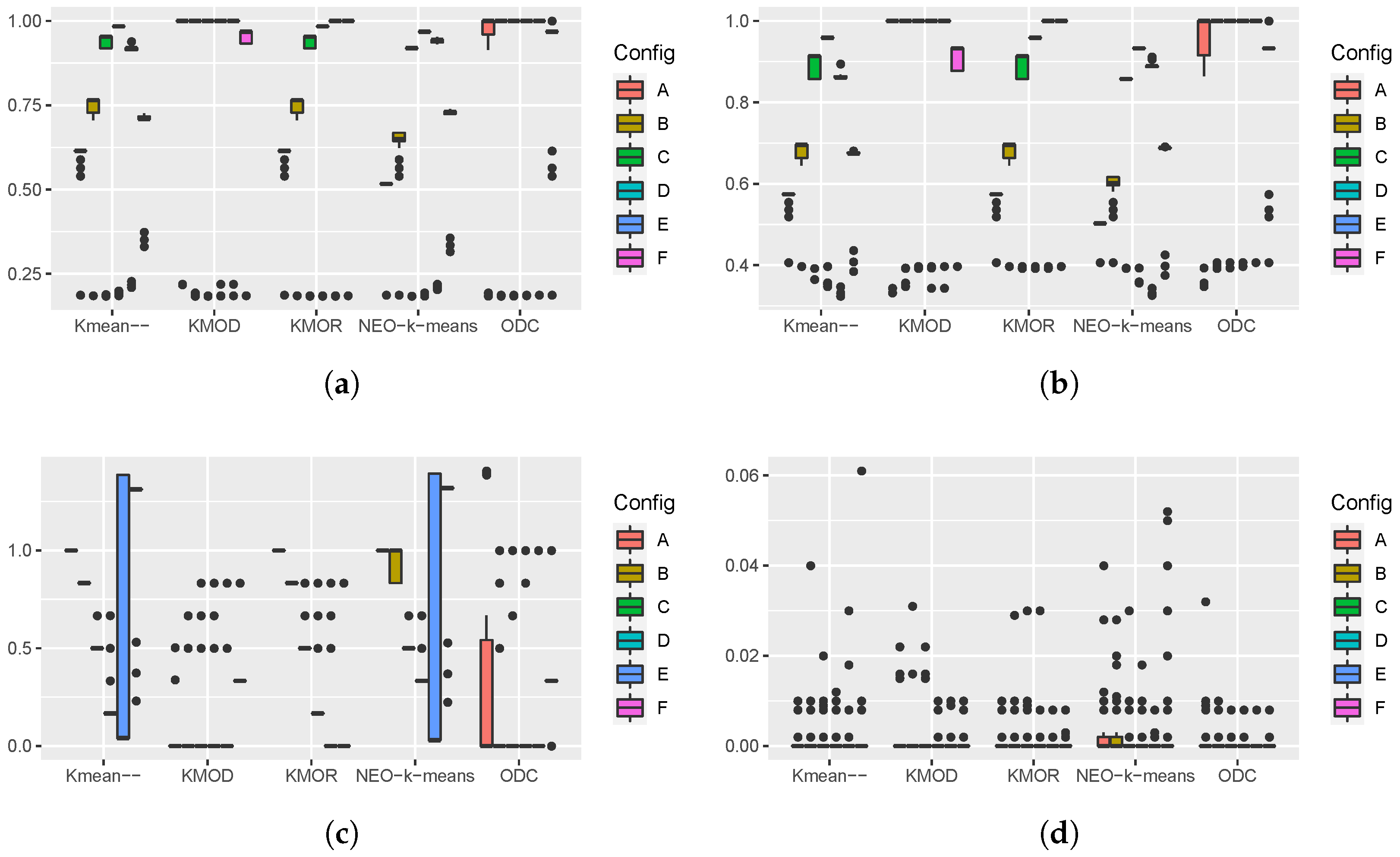
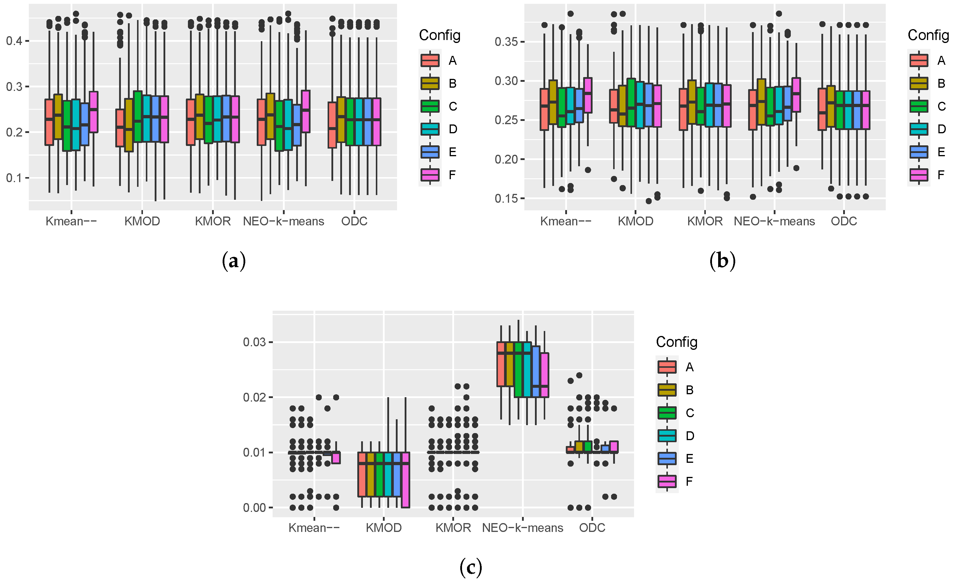
Figure 3 shows the boxplots of the performance measures obtained from 100 runs of the five algorithms on the second synthetic dataset. The boxplots of the AIR and the NMI show that the five algorithms have a similar median performance in most cases. For parameter configuration A, the KMOD algorithm obtained the best performance and the ODC had the worst performance. The boxplots of the classifier distance show that, for parameter configurations A and B, the KMOD algorithm achieved the best performance. From the boxplots of the runtime, we can see that NEO-k-means is the slowest algorithm. The other four algorithms have similar runtimes.

From the boxplots of the classifier distances shown in Figure 3c, we can see some interesting patterns regarding the performance of these algorithms in terms of outlier detection. The k-means-- algorithm and the NEO-k-means algorithm use a percentage of the total number of data points to control the number of outliers. From parameter configurations A to B, the percentage increases from 0% to 20%. We can see that the median classifier distance of k-means-- and NEO-k-means decreases from the parameter configuration A to B. This pattern indicates that a large percentage parameter value is needed to include the outliers. The pattern of KMOR is not monotonic because the number of outliers is controlled by the interaction between two parameters. The pattern of ODC shows jumps and does not change gradually because the data points identified as outliers in ODC cannot become normal points anymore. The pattern of KMOD shows gradual changes when parameter $\gamma$ increases from 2 to 7. The median classifier distance was the lowest when $\gamma$ was set to 2. The experiment on the second synthetic data shows that using $\gamma =2$ as the default parameter value is a good choice.

4.4. Results on Real Data

We obtained several real datasets from the UCI machine learning Repository [31] to compare the performance of the KMOD algorithm and the other four algorithms.

Table 3. Summaries of the real datasets. Here, n, d, and k denote the number of records, the number of attributes, and the number of classes of the corresponding dataset, respectively.

	n	d	k
Wine	178	13	3
Gesture phase	1747	18	5
Anuran calls	7195	22	10
Shuttle	43,500	9	7

presents some information about these real datasets. The real datasets have different sizes and different dimensionalities.

The wine dataset contains records from three different origins, which can be used as classes for the purpose of cluster analysis. The gesture phase dataset contains records extracted from videos of people gesticulating. The anuran calls dataset contain records created by segmenting 60 audio records that belong to four different families, eight genera, and ten species. In our experiments, we divided the dataset into 10 clusters, each of which represents a species. The shuttle dataset is a relatively large dataset that contains 58,000 records. The shuttle dataset consists of a training set and a test set. In our experiments, we used the training set that contains 43,500 records from seven classes.

Since the real datasets do not have labels for outliers, we assigned the outliers found by the clustering algorithms to their nearest cluster centers before calculating the two performance measures: the ARI and the NMI. As a result, we did not calculate the classifier distances for real datasets.

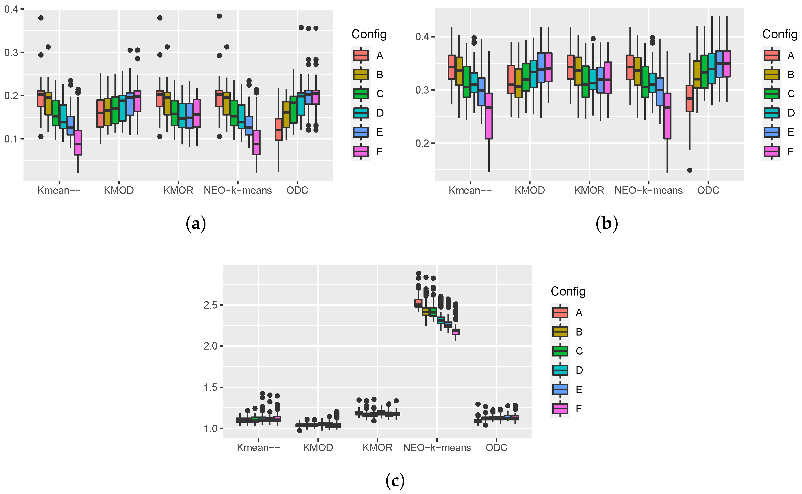
Figure 4 shows the boxplots of the performance measures produced by 100 runs of the five algorithms on the wine dataset. The boxplots of the ARI and the NMI show that the KMOD algorithm and the KMOR algorithm had a similar performance on the wine dataset. However, the KMOD algorithm outperformed the KMOR algorithm when parameter configurations A to C were used. Since the wine dataset is small, all algorithms converged quickly in most cases.

Figure 5 shows the boxplots of the performance measures obtained from 100 runs of the five algorithms on the gesture phase dataset. From the boxplots of the ARI and the NMI, we see that all five algorithms achieved a similar performance on this dataset in terms of accuracy. Since the gesture phase dataset is relatively large, we can see the runtime differences in the boxplots of the runtime. The NEO-k-means algorithm was the slowest of the five algorithms. If we look at the median runtime, we can see that the KMOD algorithm was the fastest of the five algorithms.

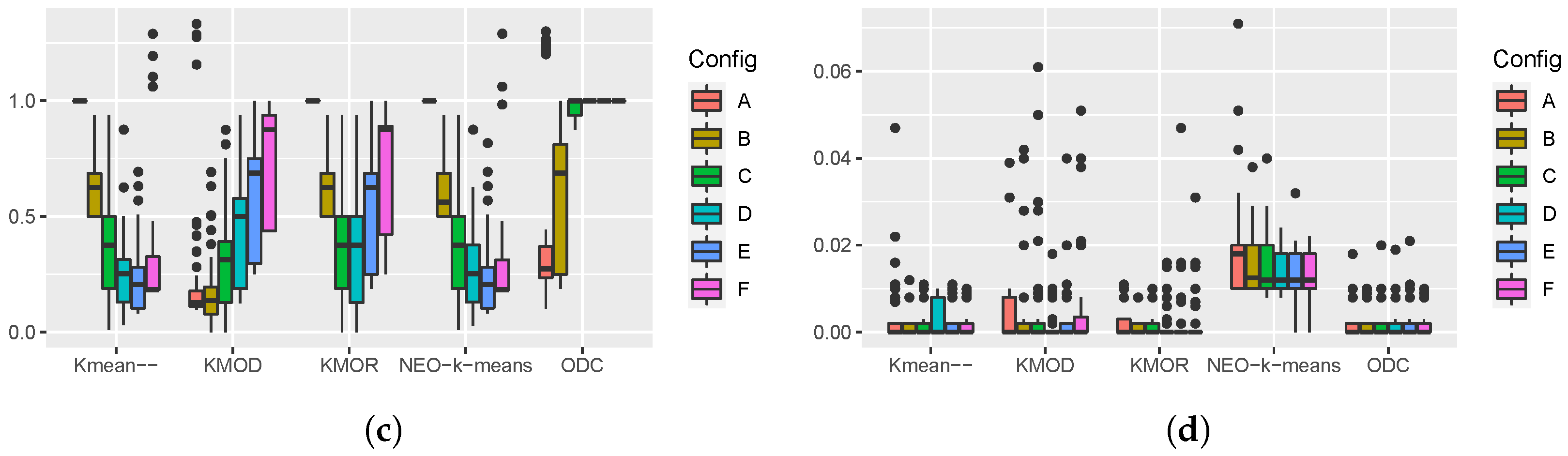
Figure 6 shows the boxplots of the performance measures produced by 100 runs of the five algorithms on the anuran calls dataset. From the boxplots of the ARI and the NMI, we see that the KMOD algorithm and the KMOR algorithm have a similar average performance. When the parameter configuration F was used, the average accuracy of the k-means-- algorithm and the NEO-k-means algorithm decreased. The boxplots of the runtime shows that the NEO-k-means algorithm was the slowest algorithm. The average runtime was similar for the other four algorithms.

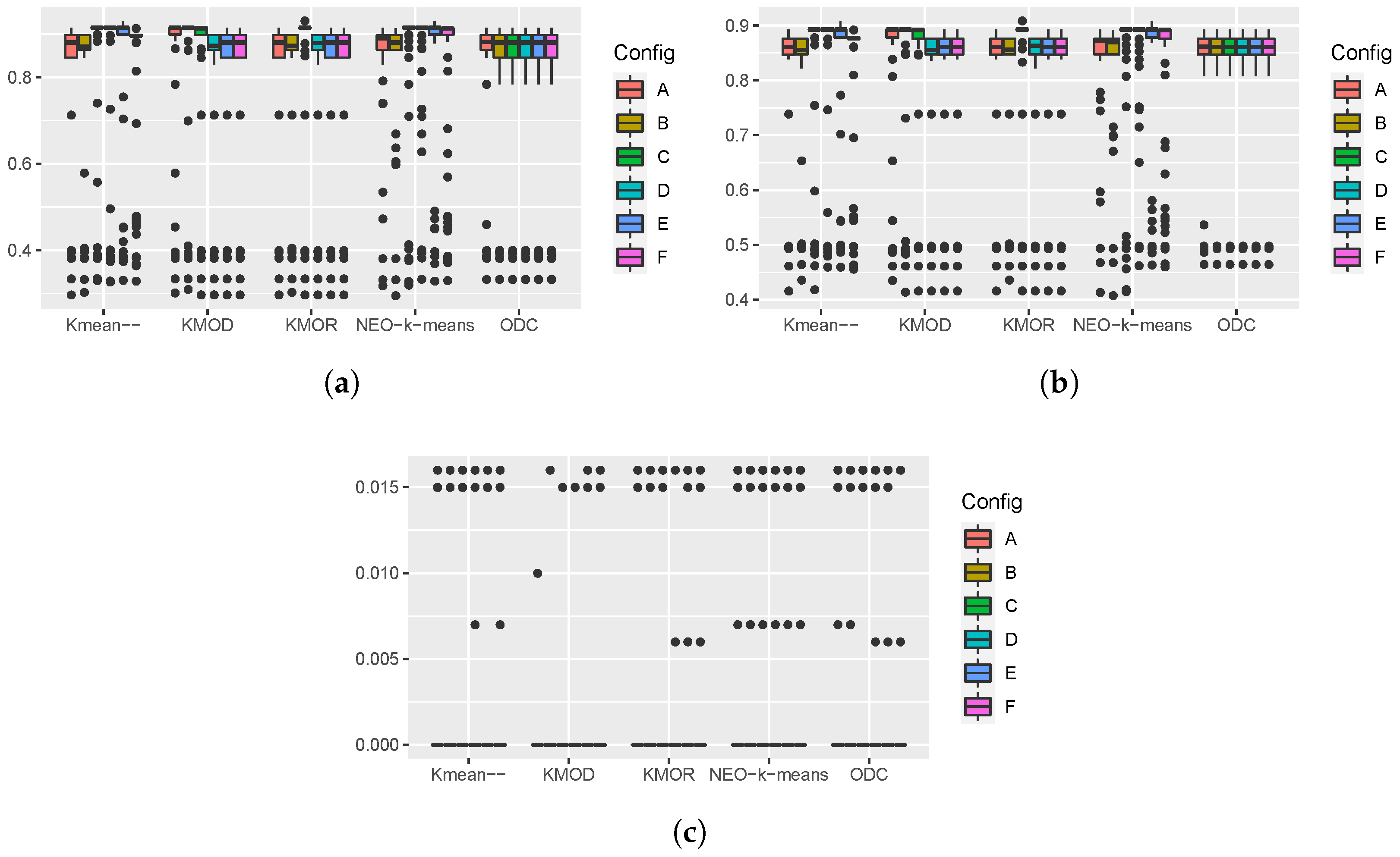
Figure 7 shows the boxplots of the performance measures produced by 100 runs of the five algorithms on the shuttle dataset. From the boxplots of the ARI and the NMI, we can see that the KMOD algorithm achieved the best overall performance across the different parameter configurations. The performance of k-means--, NEO-k-means, and ODC varied a lot across different parameter configurations.

From the boxplots of the runtime, we can see that the KMOD algorithm was the fastest of the five algorithms when applied to this dataset, which is a relatively large dataset. We expect the KMOD algorithm to be faster than the KMOR algorithm because the latter sorts distances to find outliers to satisfy the constraints imposed by the algorithm. In the KMOD algorithm, distance sorting is not required.

In summary, the experiments on synthetic data showed that the KMOD algorithm is able to cluster data and detect outliers simultaneously. The experiments on real data showed that the KMOD algorithm is able to achieve a better overall performance and is faster than other algorithms. The experiments on real data also showed that the KMOD algorithm is not sensitive to the parameter used to control the number of outliers.

5. Conclusions

In this paper, we proposed a KMOD algorithm that is able to perform data clustering and outlier detection simultaneously. In the KMOD algorithm, outlier detection is a natural part of the clustering process. This is achieved by introducing an “outlier” cluster that contains all the points that are considered outliers. The KMOD algorithm produces two partition matrices: one partition matrix divides a dataset into k clusters and an “outlier” cluster and the other partition matrix divides a dataset into k clusters without labeling outliers. As a result, the KMOD algorithm can be used to detect outliers and can also be used like a normal clustering algorithm.

An advantage of the KMOD algorithm is that it requires only one parameter to control the number of outliers. This parameter is intuitive in that it is a distance threshold to determine whether a data point is an outlier. As a result, setting a value for this parameter is straightforward for any dataset.

We compared the KMOD algorithm with other four similar algorithms (i.e., k-means--, KMOR, NEO-k-means, and ODC) using both synthetic datasets and real datasets. The test results have shown that the KMOD algorithm outperformed the other algorithms in terms of accuracy and speed. In particular, the KMOD algorithm was less sensitive to the parameter used to control the number of outliers than other algorithms.

The KMOD algorithm is a variant of the k-means algorithm. As a result, the KMOD algorithm inherits the advantages as well as the disadvantages of the k-means algorithm. The KMOD algorithm is simple to implement and can be used in applications where the k-means algorithm is used. Like the k-means algorithm, the KMOD algorithm is also sensitive to initial cluster centers. Other efficient cluster center initialization methods [32] can be used to improve the KMOD algorithm.

It is worth mentioning that outliers can also be handled before clustering algorithms are applied. For example, Fränti and Yang [33] proposed a data cleaning procedure that employs a medoid shift to reduce noise in the data prior to clustering. This method processes each data point by computing its k-nearest neighbors (k-NN) and replacing the point with the medoid of its neighborhood. Another example in this line of research is the mean-shift outlier detection method proposed by Yang et al. [34].