Modeling and Multi-Objective Optimization of Transcutaneous Energy Transmission Coils Based on Artificial Intelligence

Abstract
1. Introduction
- A method for modeling and optimizing TET coils is proposed, which combines the Extreme Learning Machine (ELM) with the Non-Dominated Sorting Whale Optimization algorithm (NSWOA). The ELM is used to construct a surrogate model for the multi-input and multi-output parameters of the TET coils. Based on this surrogate model, a multi-objective optimization function for the TET coils is constructed, and the NSWOA is then used to perform multi-objective optimization on the TET coils.
- To improve the modeling accuracy of the TET coils, the Gray Wolf Optimizer (GWO) was introduced and applied to the parameter tuning of the ELM model for the TET coils in this study.
- A TET coils simulation platform has been established, and the correctness of the simulation has been verified through experimental measurements. On this basis, the simulation platform was used to collect the data required for TET coil modeling.
- The proposed method was subjected to an in-depth comparative analysis with other methods through a series of evaluation metrics, fully demonstrating its effectiveness and correctness. Additionally, the optimization results obtained using the proposed method were also thoroughly validated.
2. Background
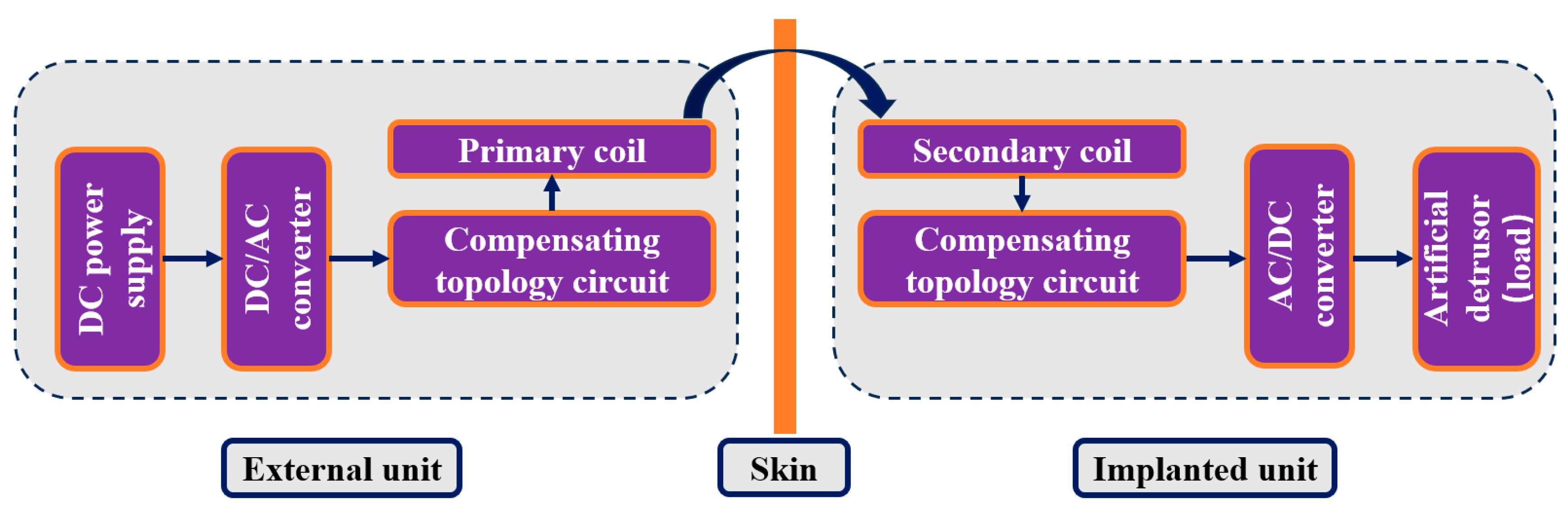
2.1. TET System Composition
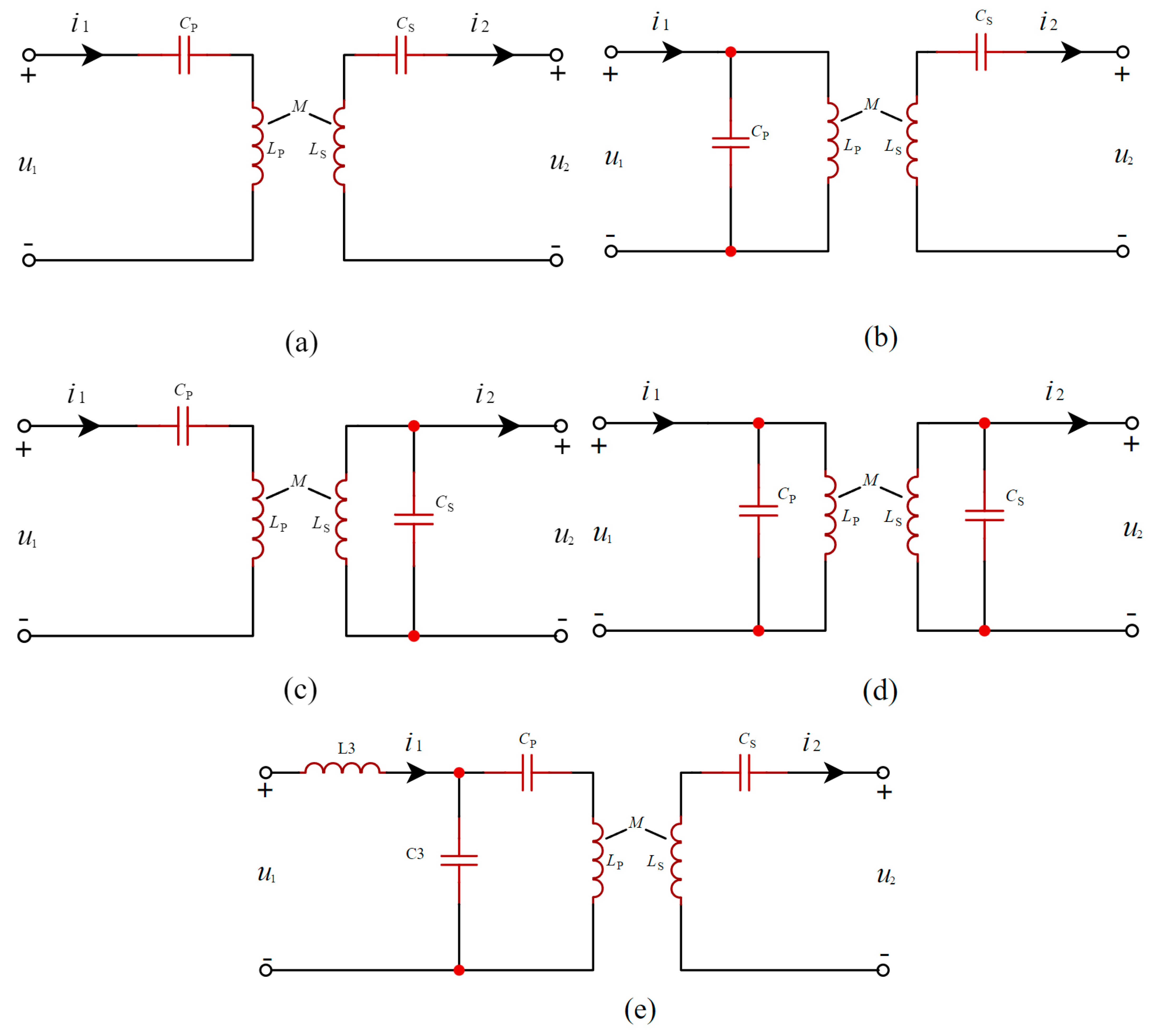
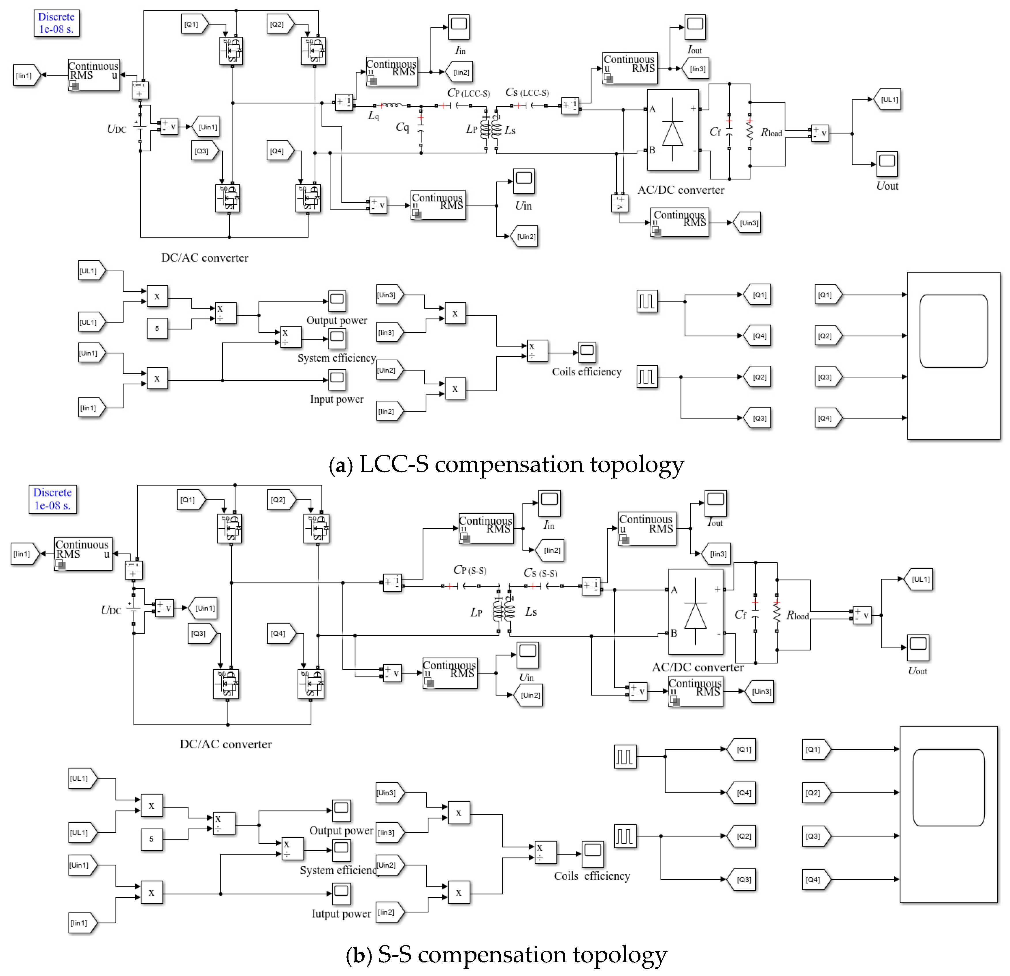
2.2. Compensating Topology Circuit
3. The Proposed Method
3.1. Data Acquisition
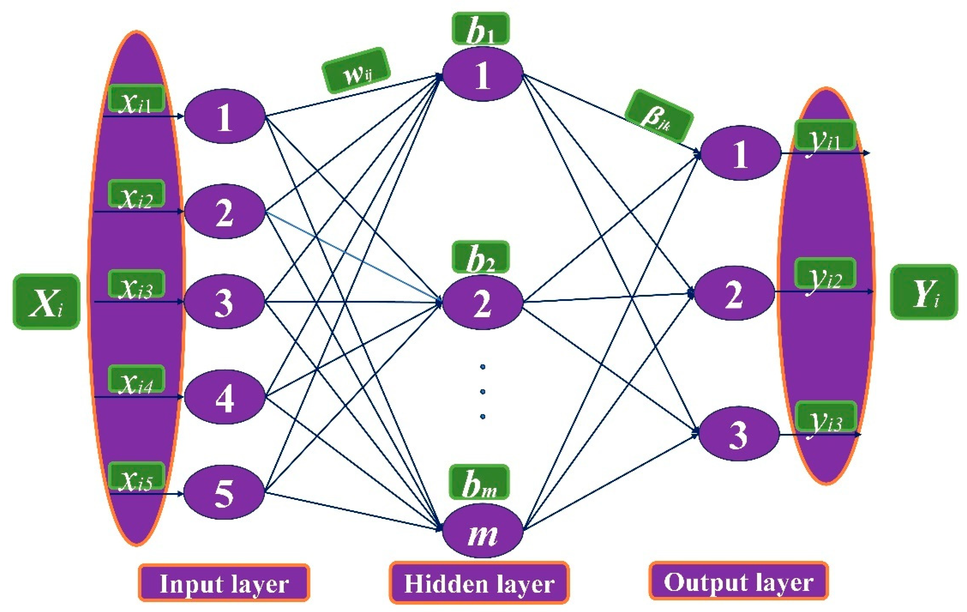
3.2. TET Coils Model Based on ELM
3.3. Metaheuristic Optimization Algorithm and ELM Parameter Tuning
3.4. Gray Wolf Optimizer
3.5. NSWOA
3.5.1. Encircling Prey
3.5.2. Spiral Bubble Net-Feeding Phase
3.5.3. Random Search for Prey
3.6. Multi-Objective Optimization Function for TET Coils
3.7. Detailed Steps and Flowchart of the Proposed Method
4. Case Validation
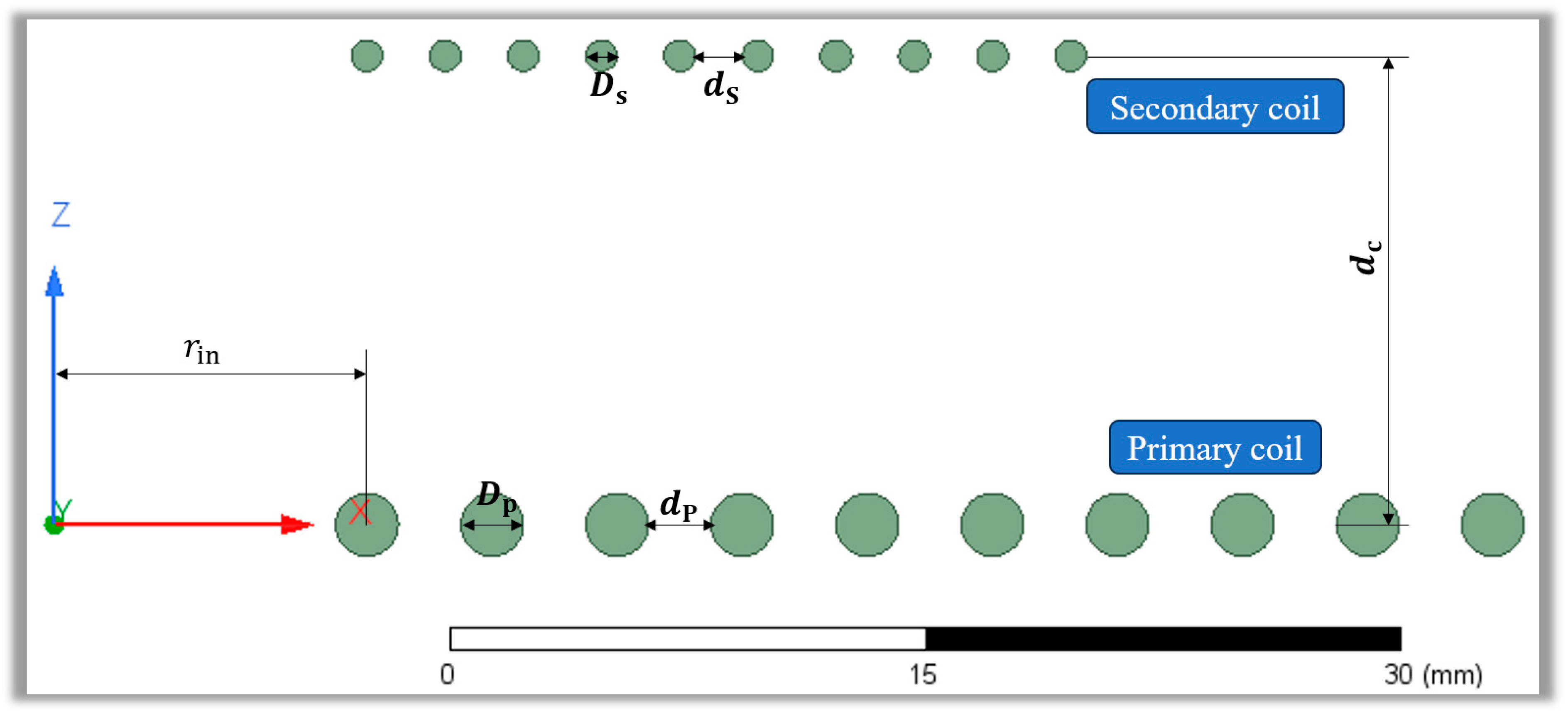
4.1. Range of Decision Variable Values
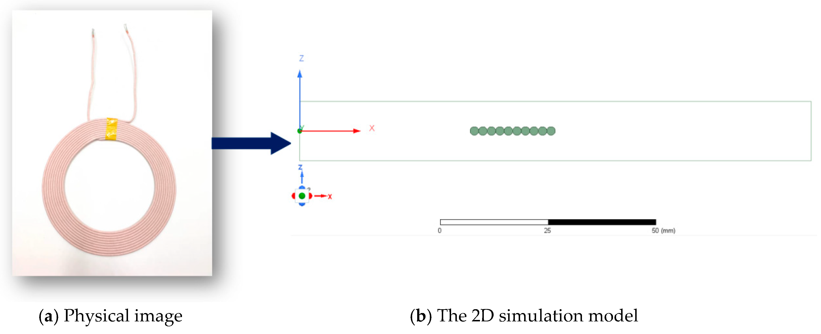
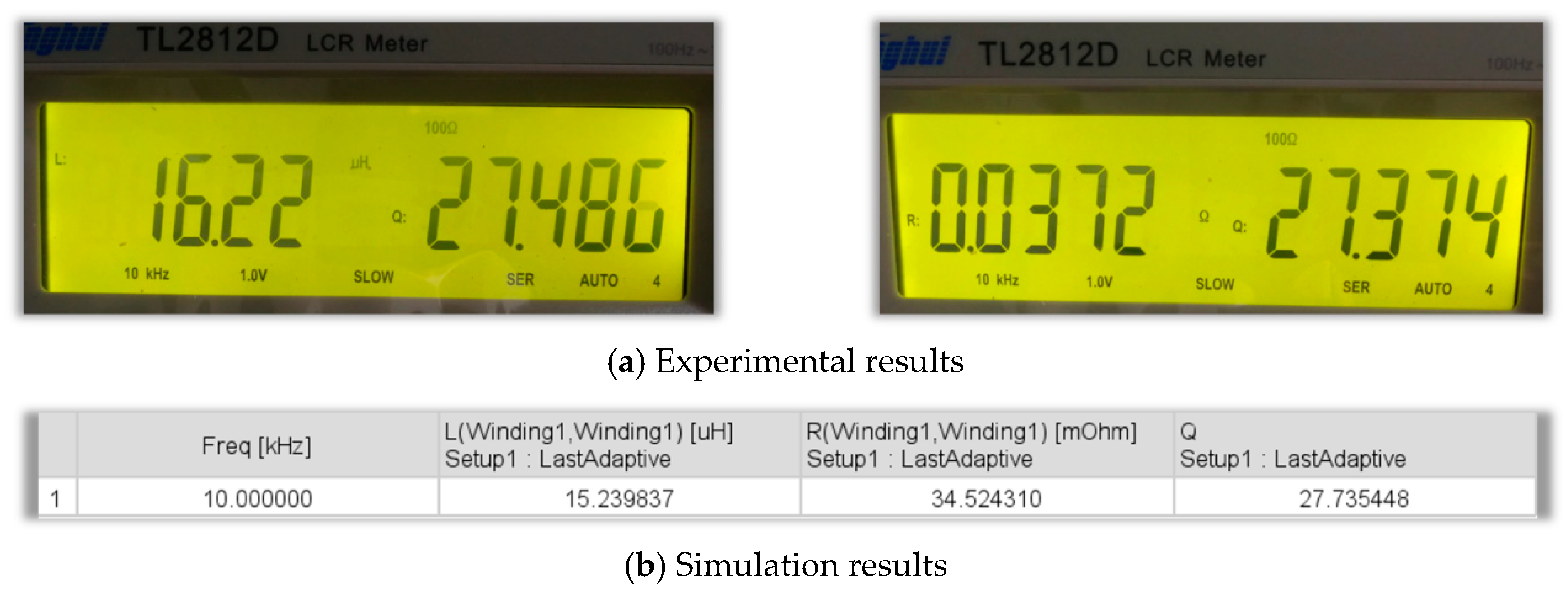
4.2. Construction and Verification of the TET Coils Simulation Platform
5. Results and Discussion
5.1. Outcome Evaluation Indexes
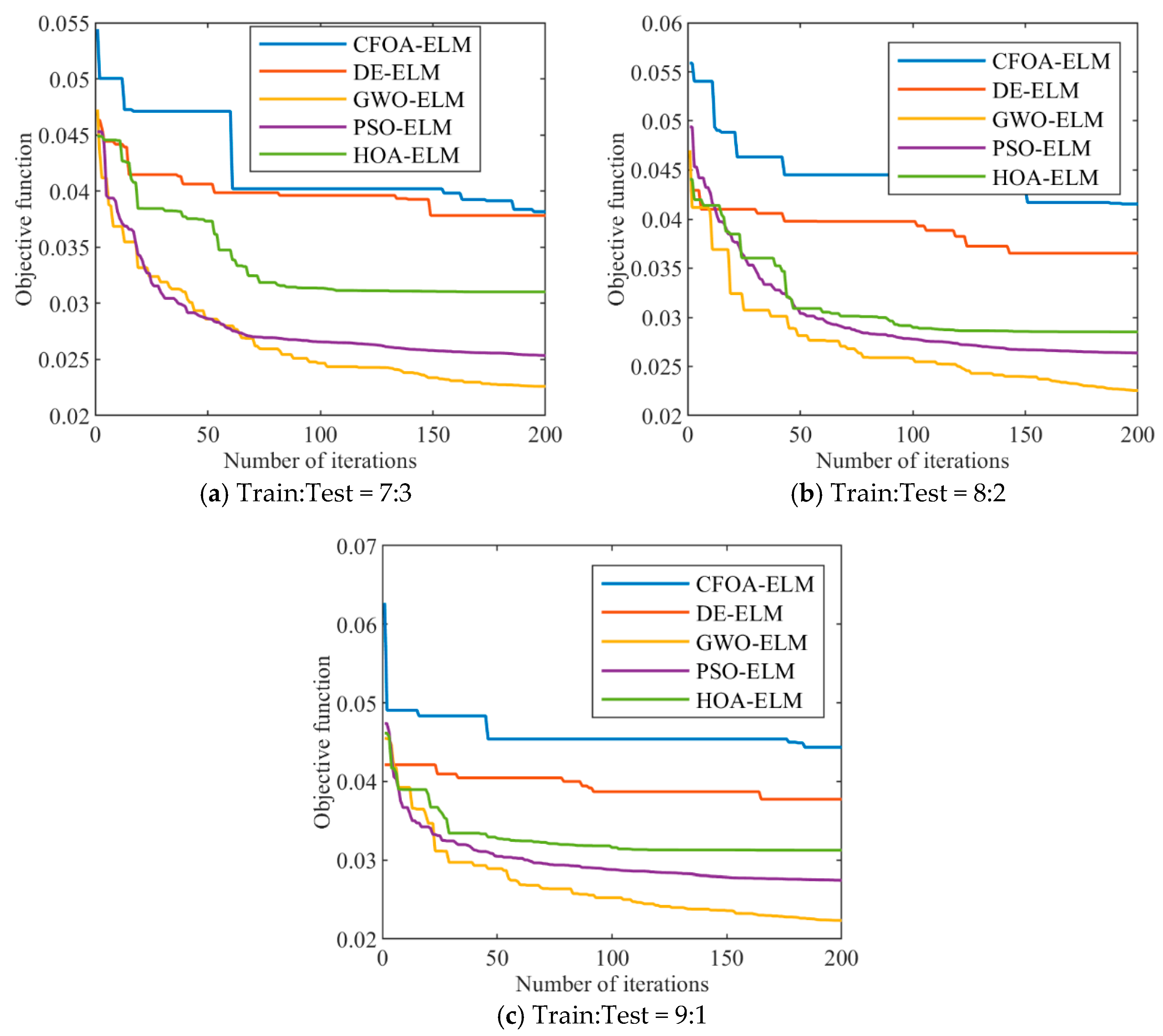
5.2. Analysis of the Optimization Performance of the GWO Algorithm in the Parameter Tuning Process of the TET Coils ELM Prediction Model
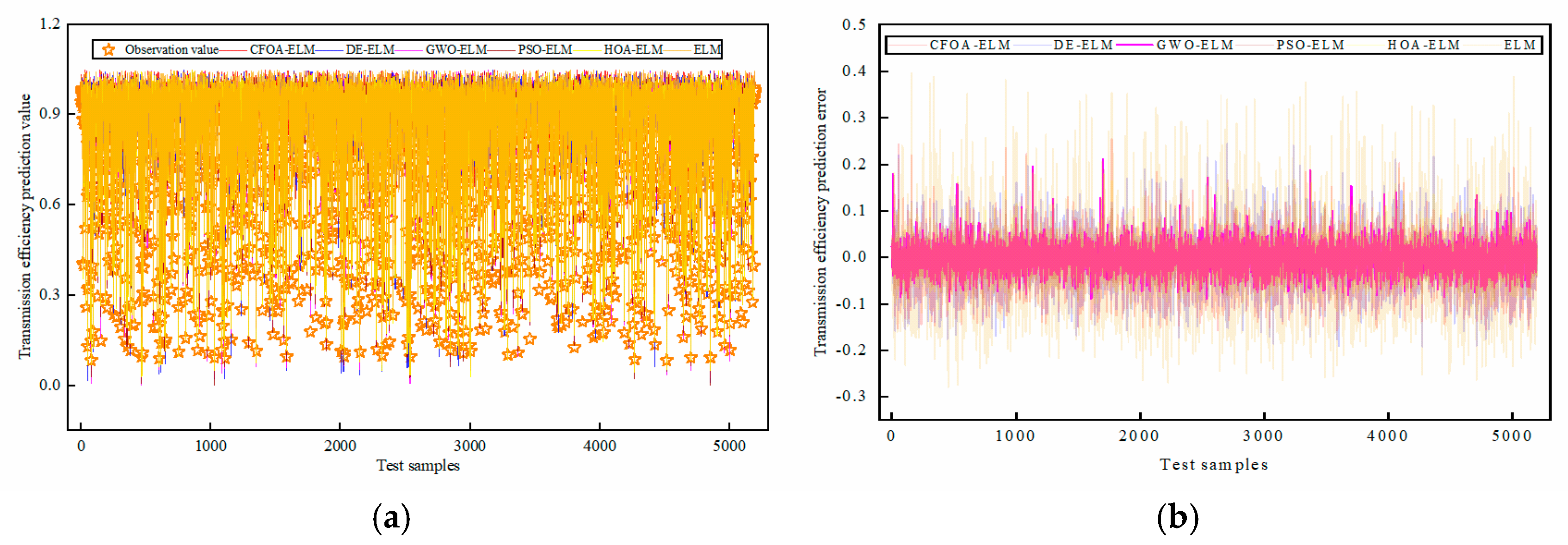
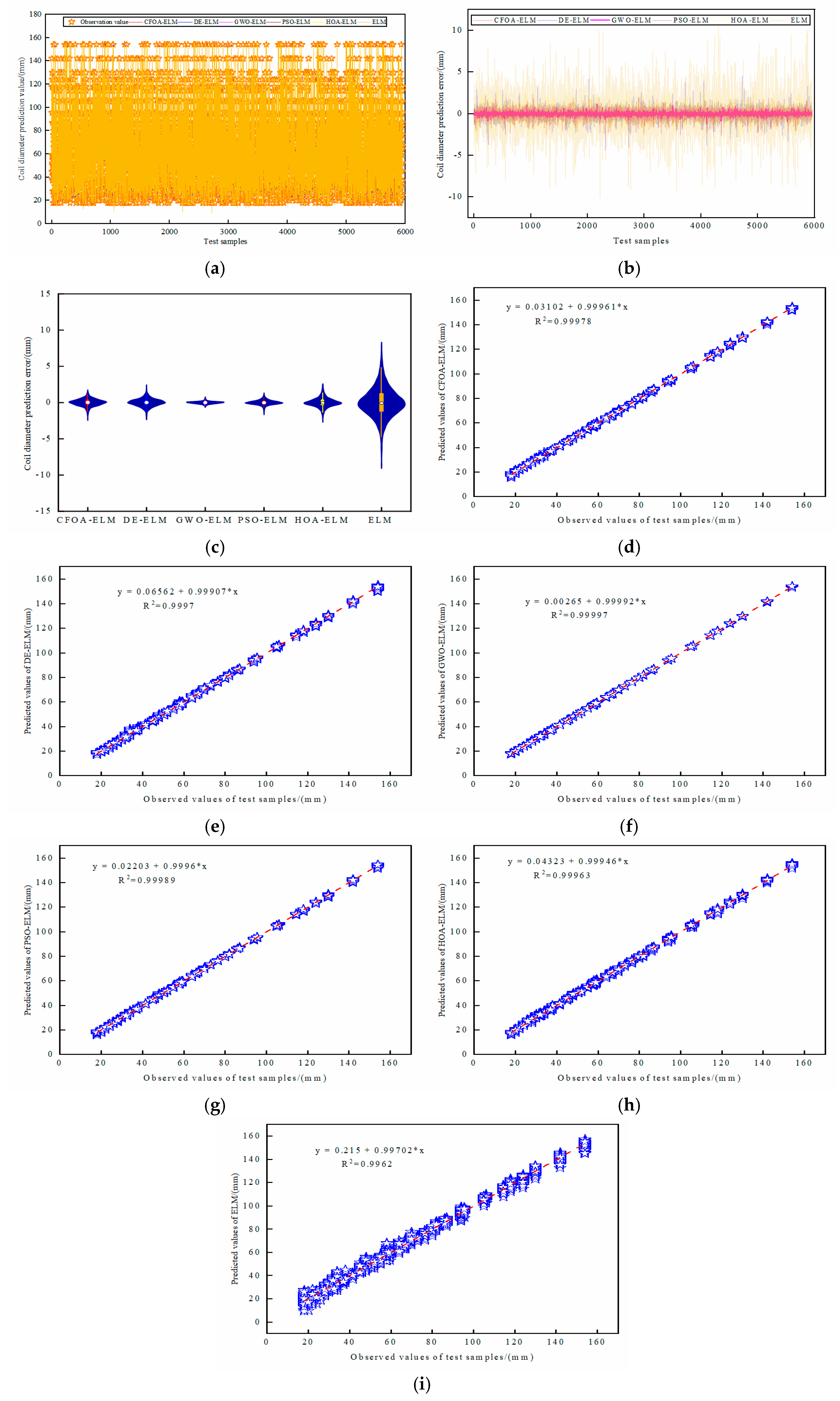
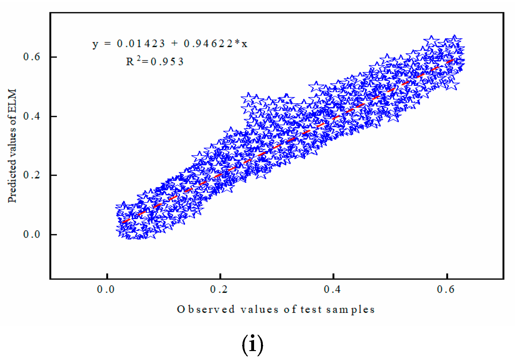
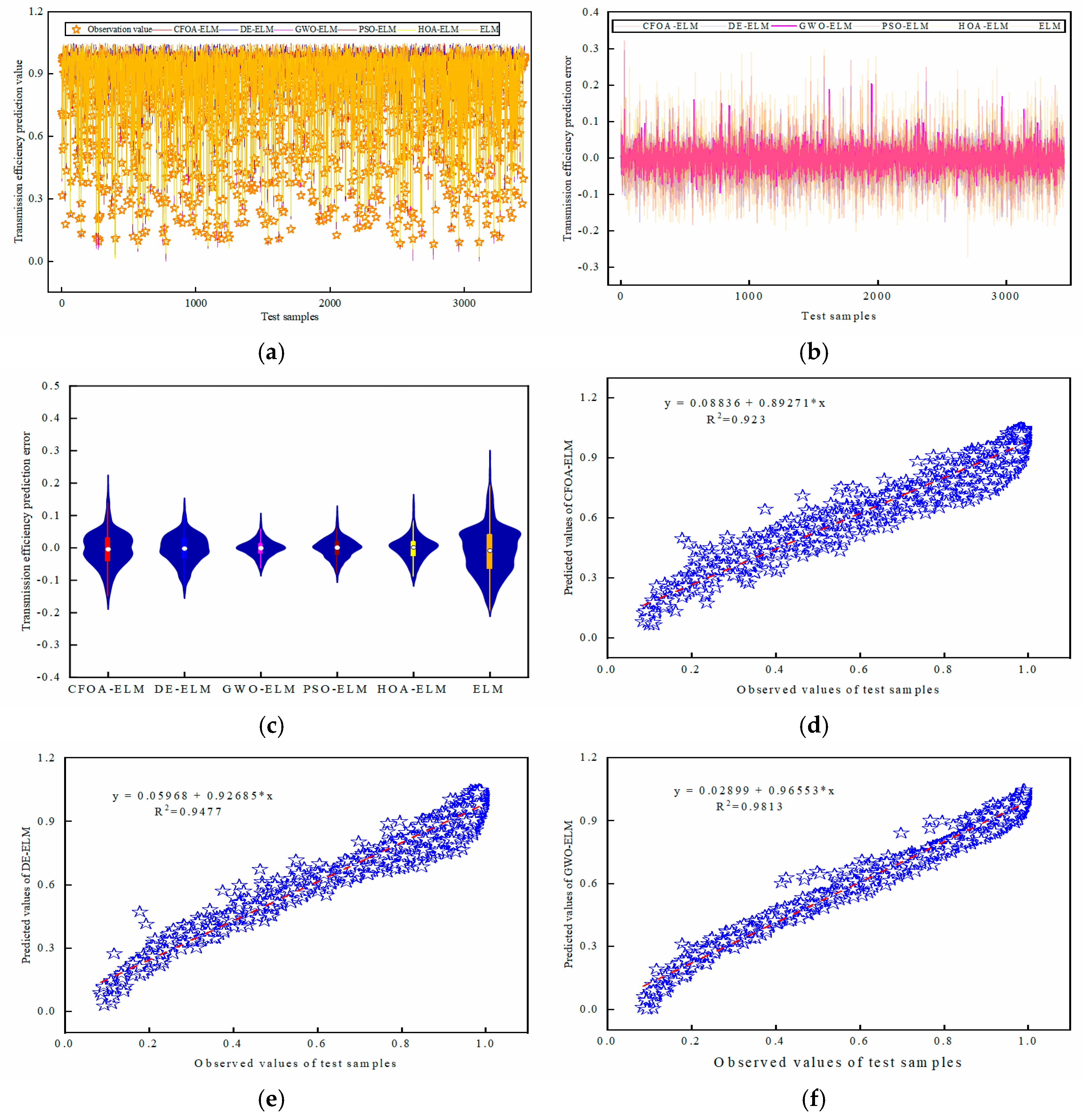
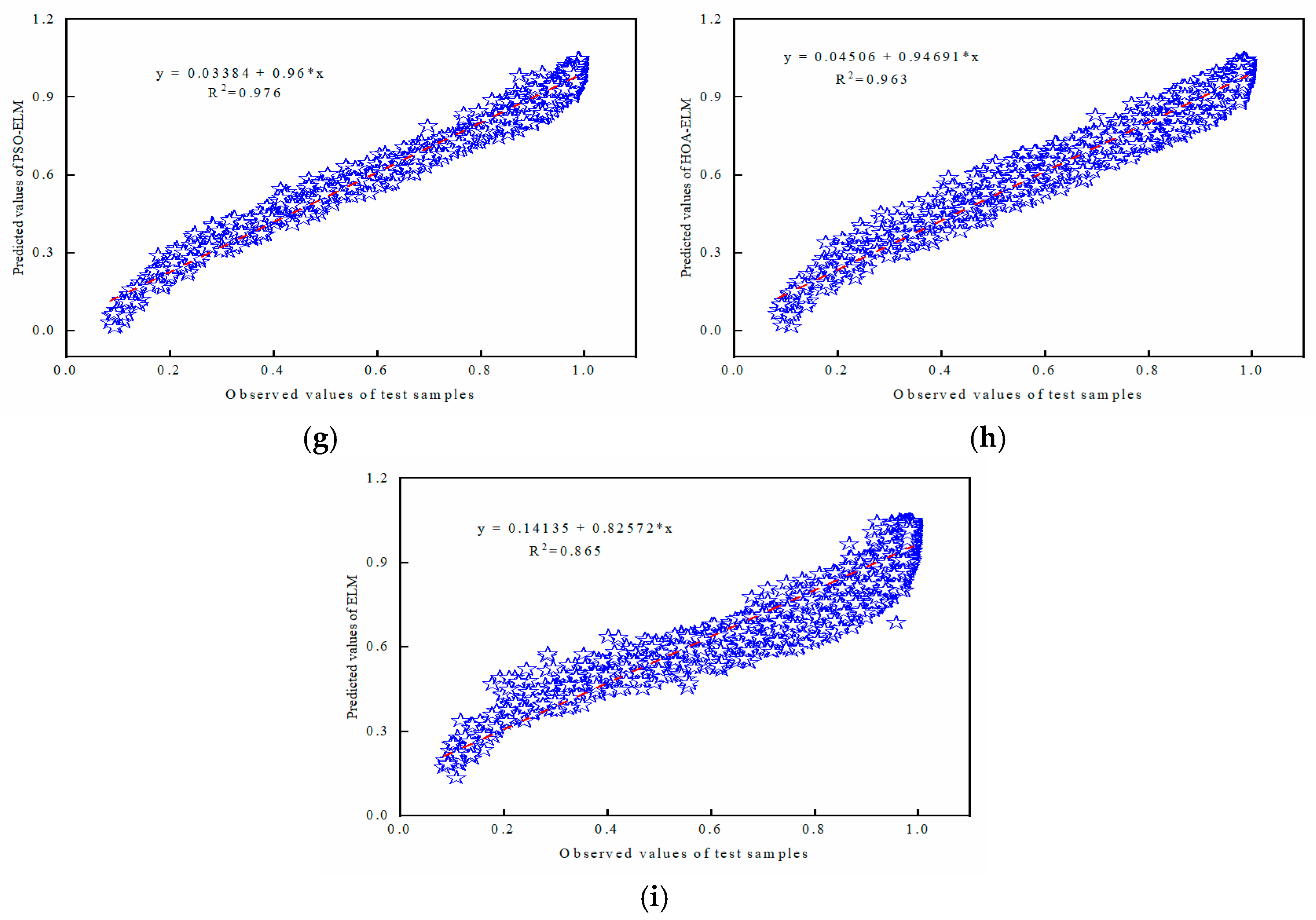
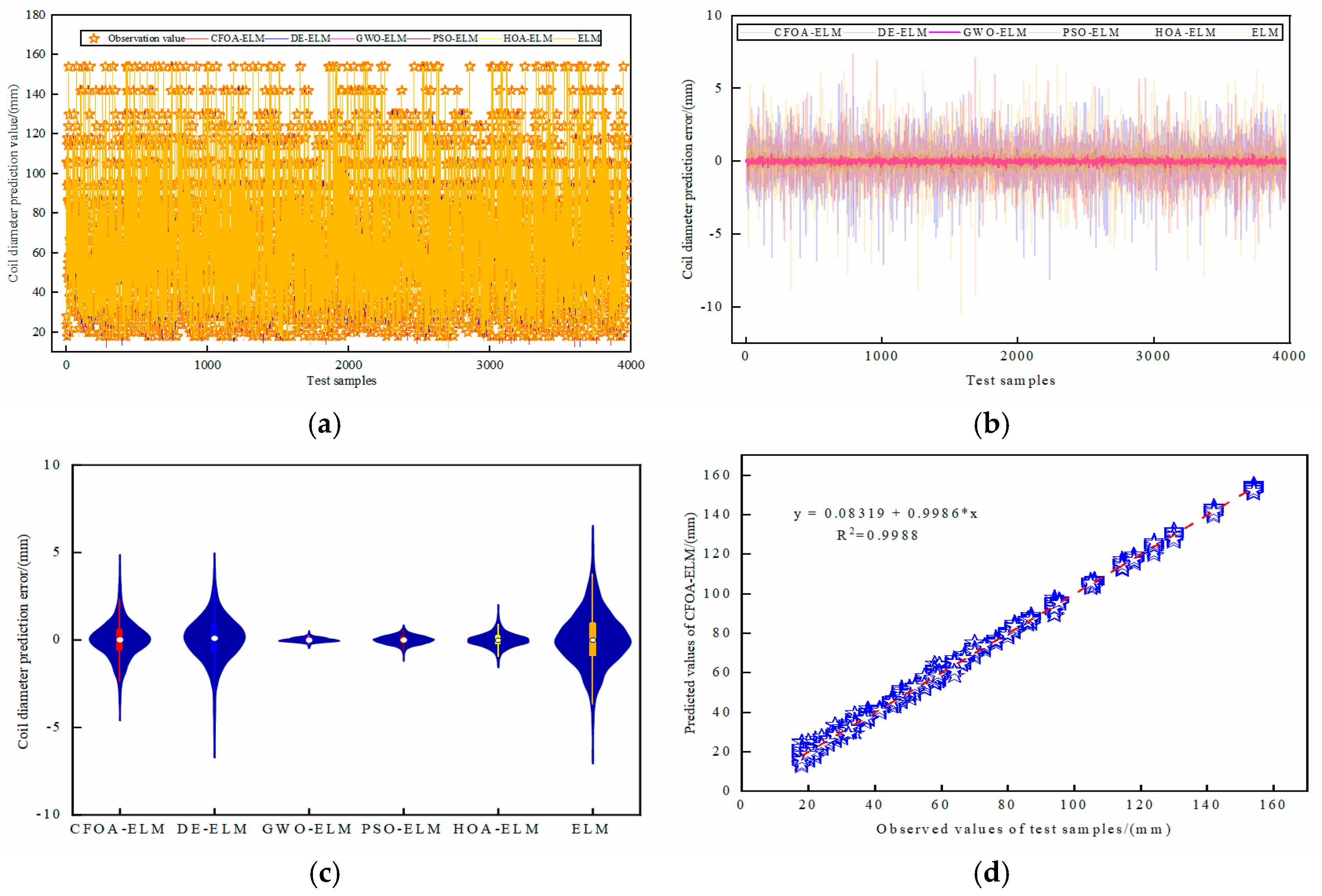
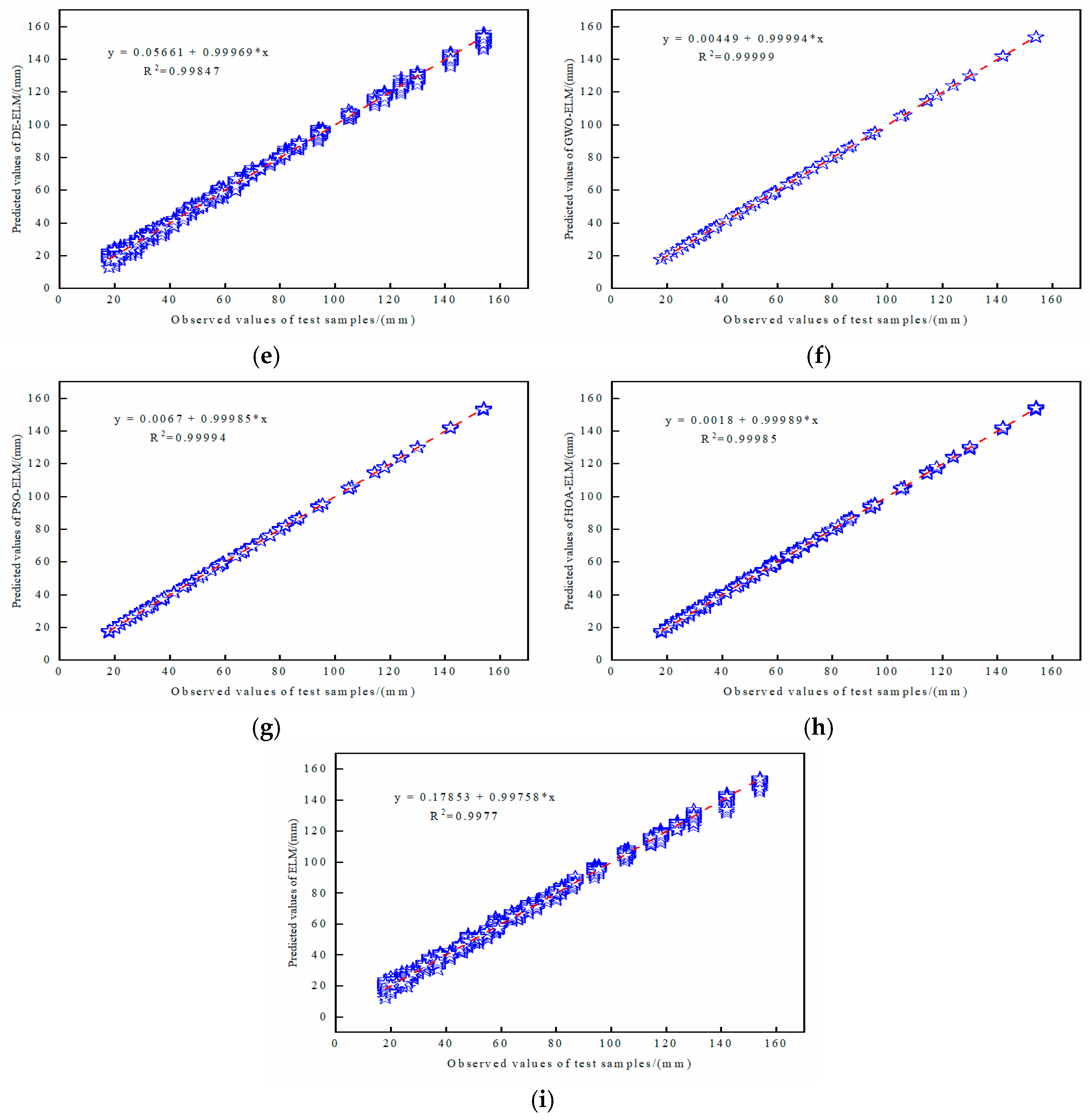
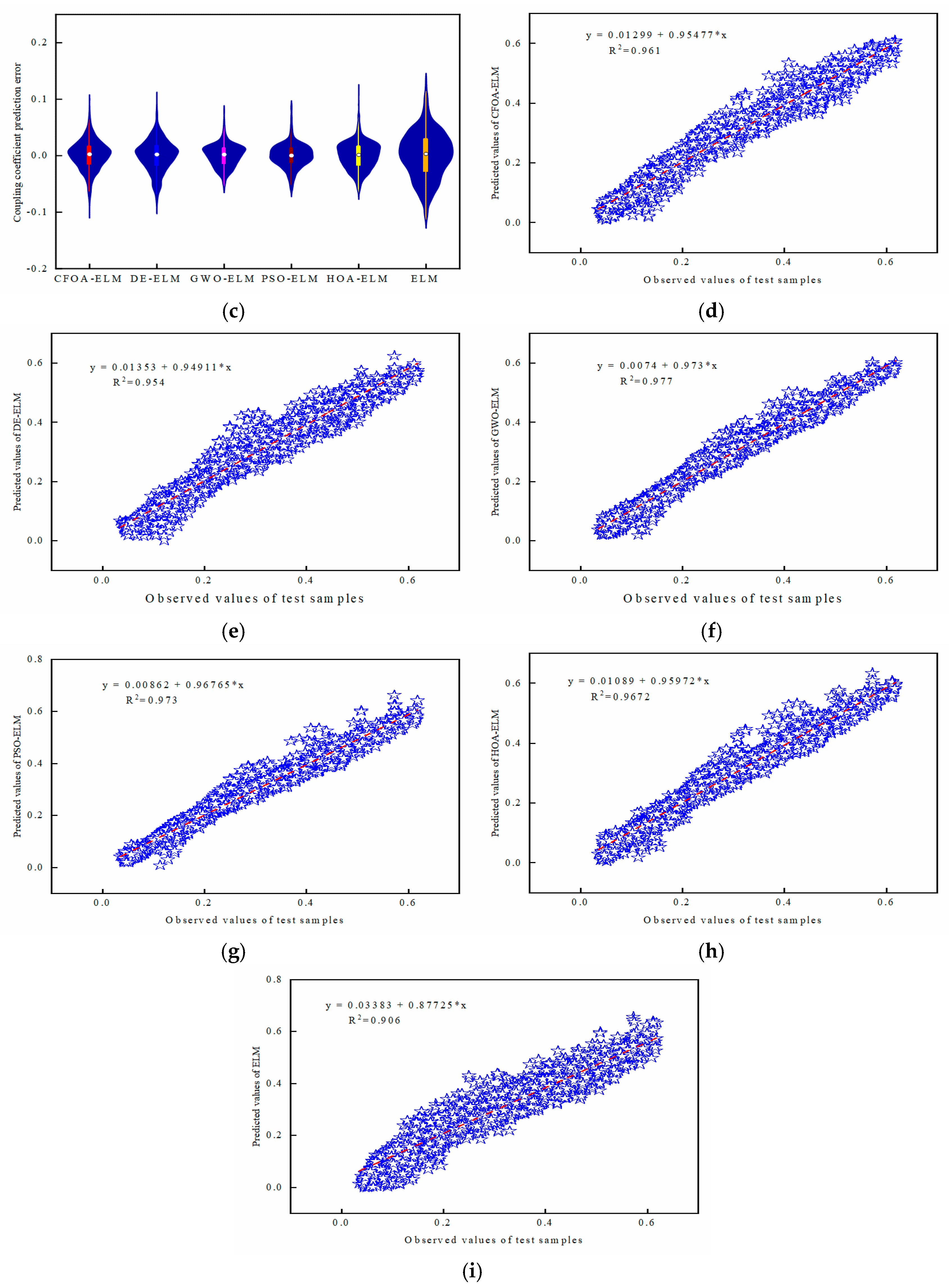
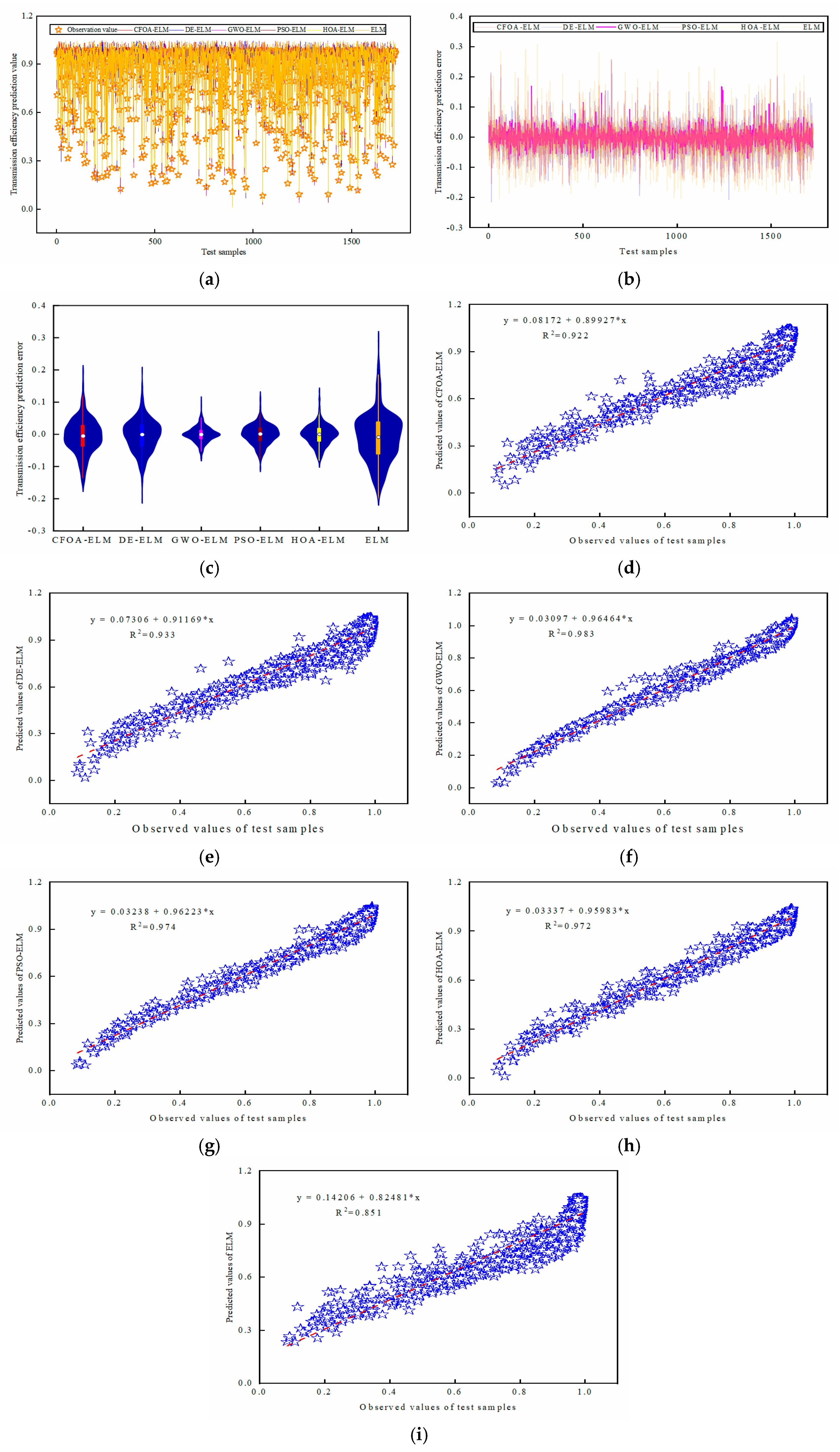
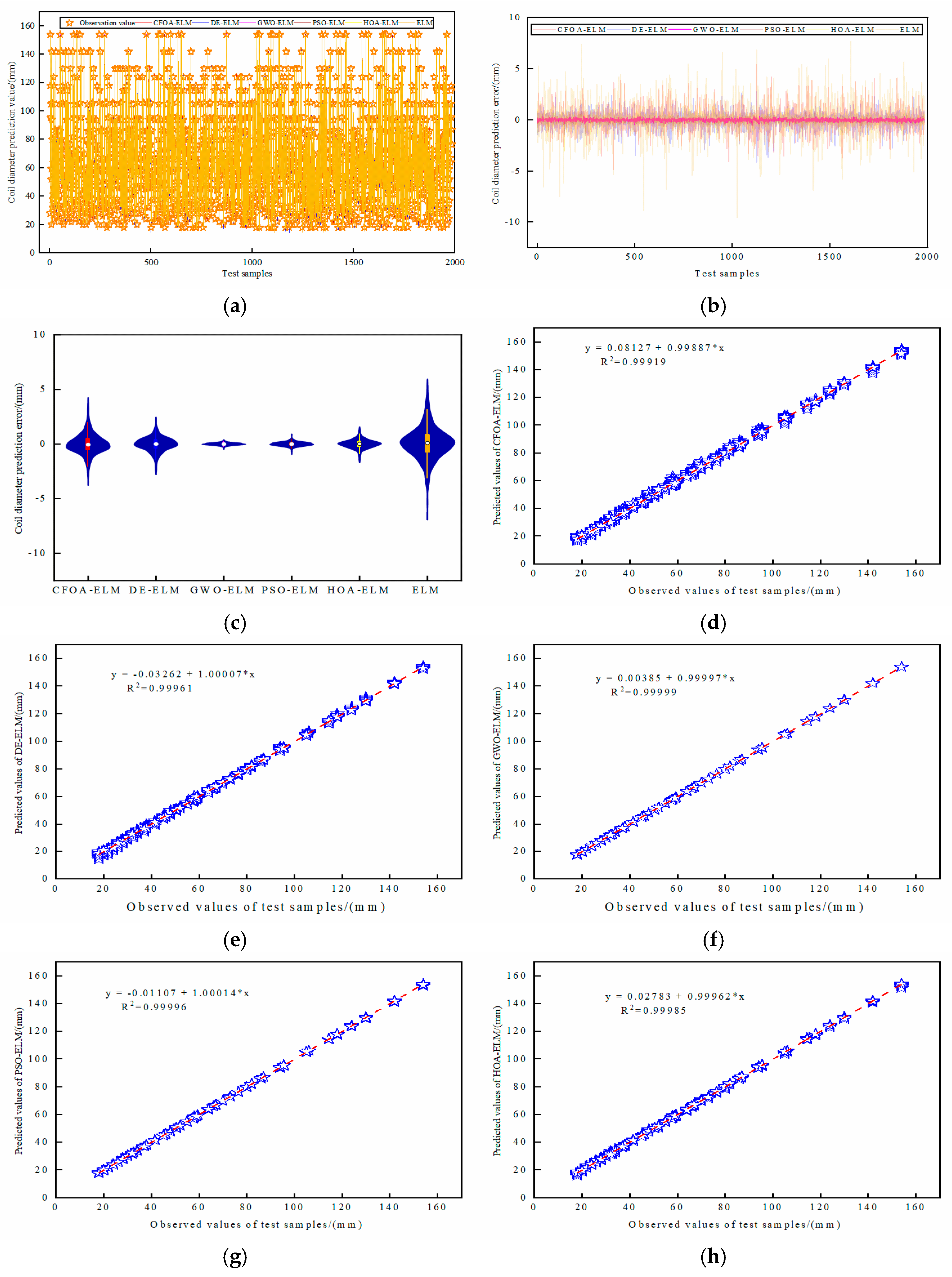
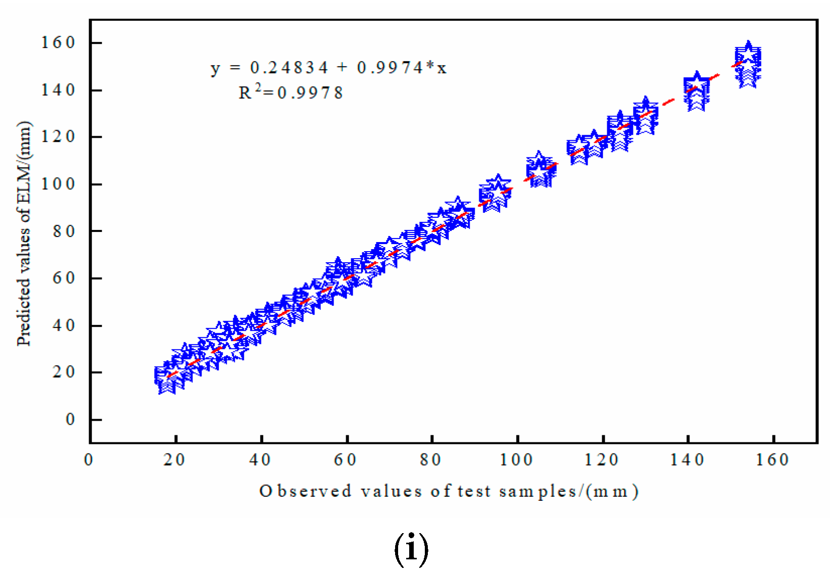
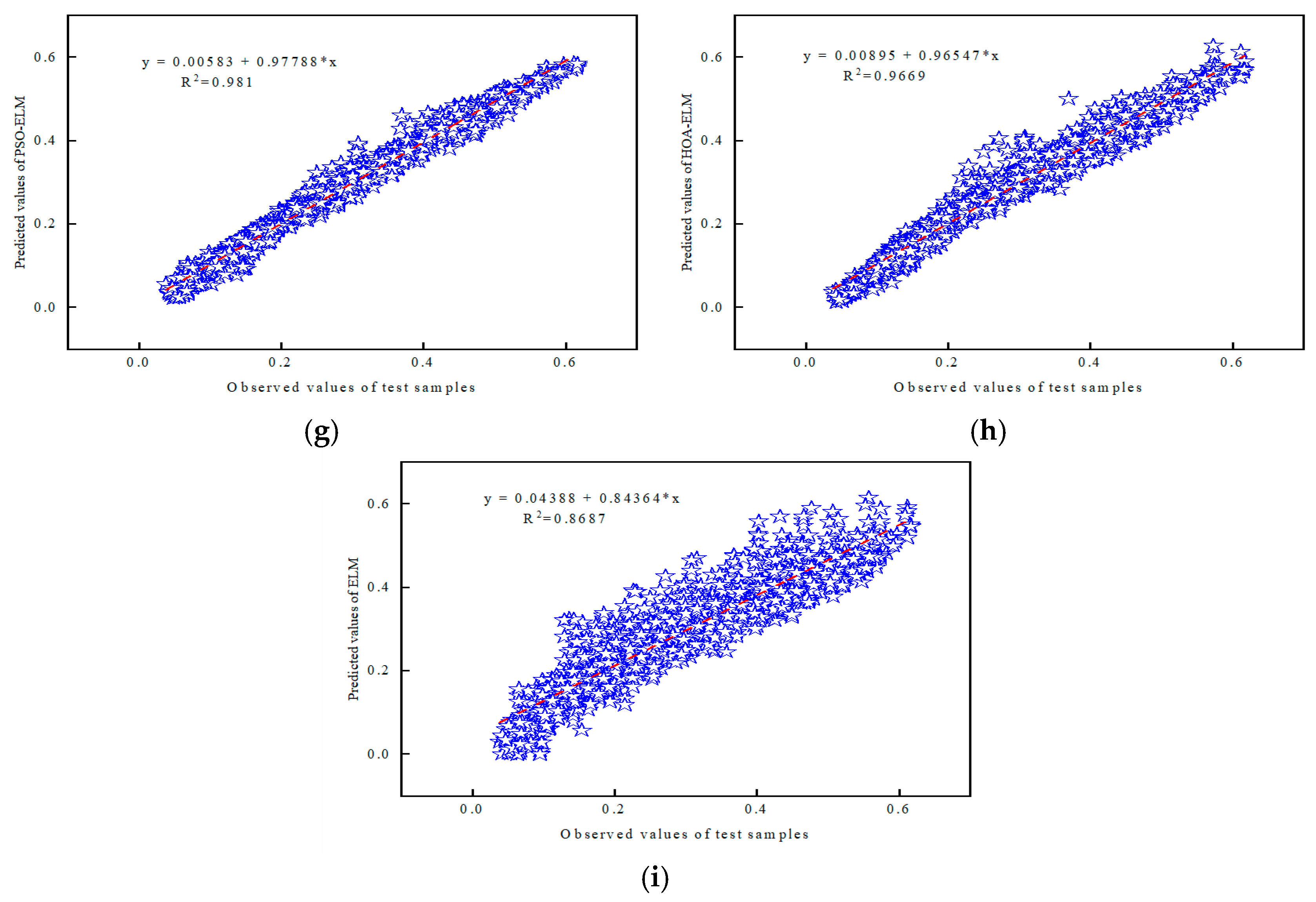
5.3. The Prediction Performance of the TET Coil GWO-ELM Prediction Model
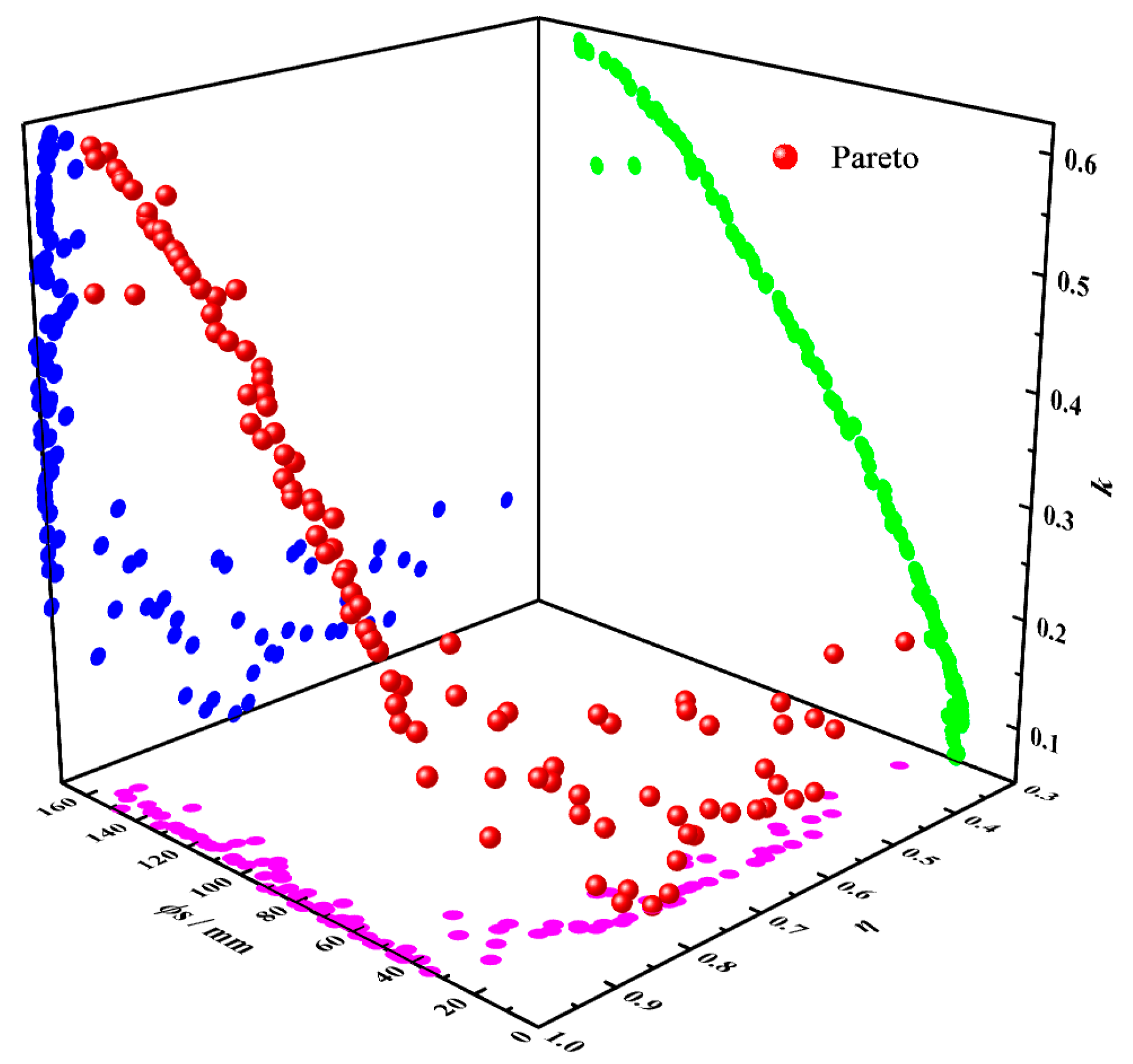
5.4. TET Coils Multi-Objective Optimization Results
5.5. Verification of the Multi-Objective Optimization Results of the TET Coils
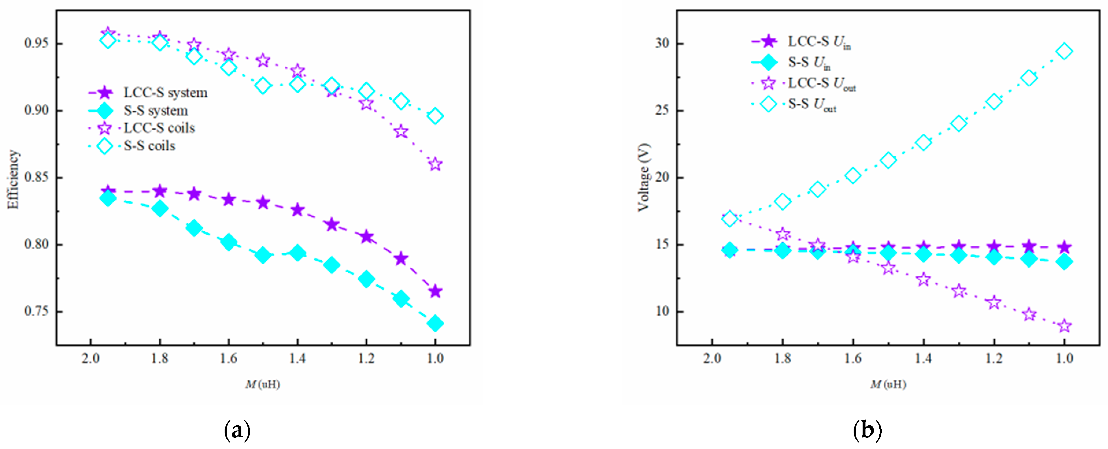
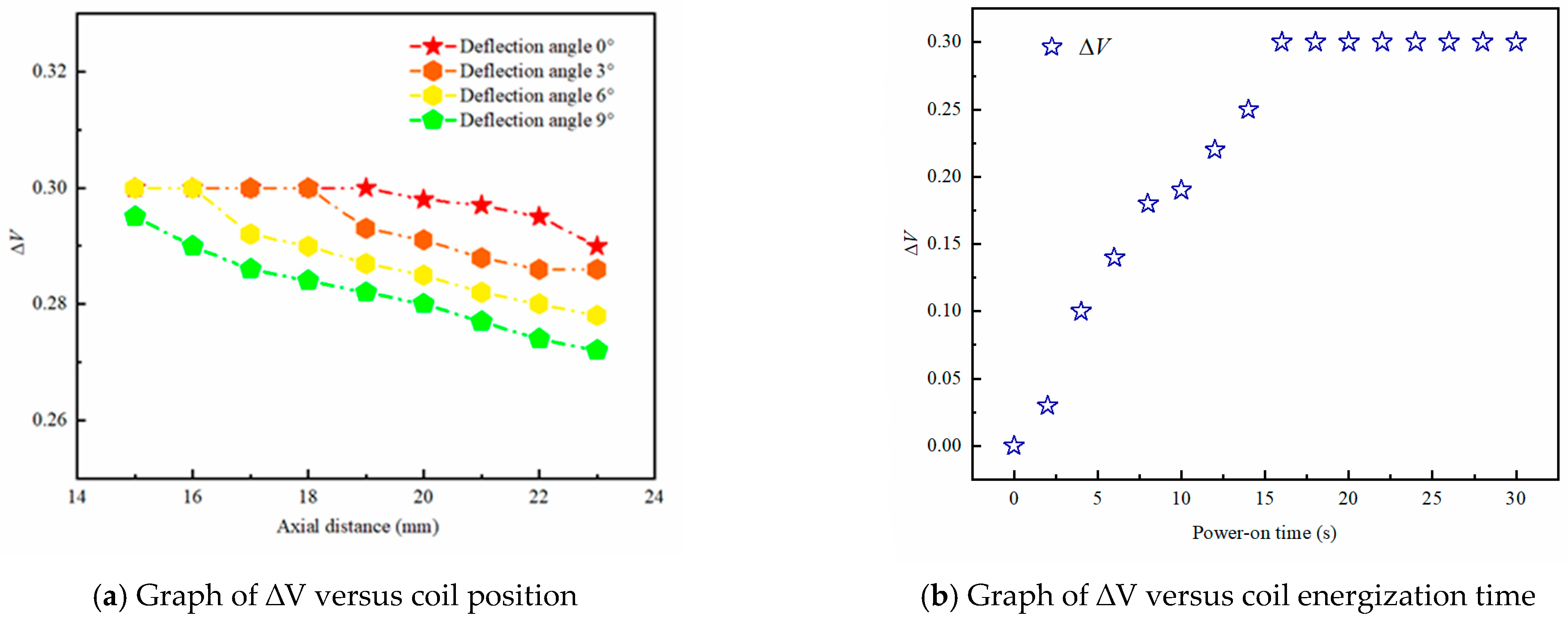
5.6. Comparison and Verification of the Anti-Misalignment Performance of the TET System Composed of the Optimal Coil Structure and Two Compensation Topologies
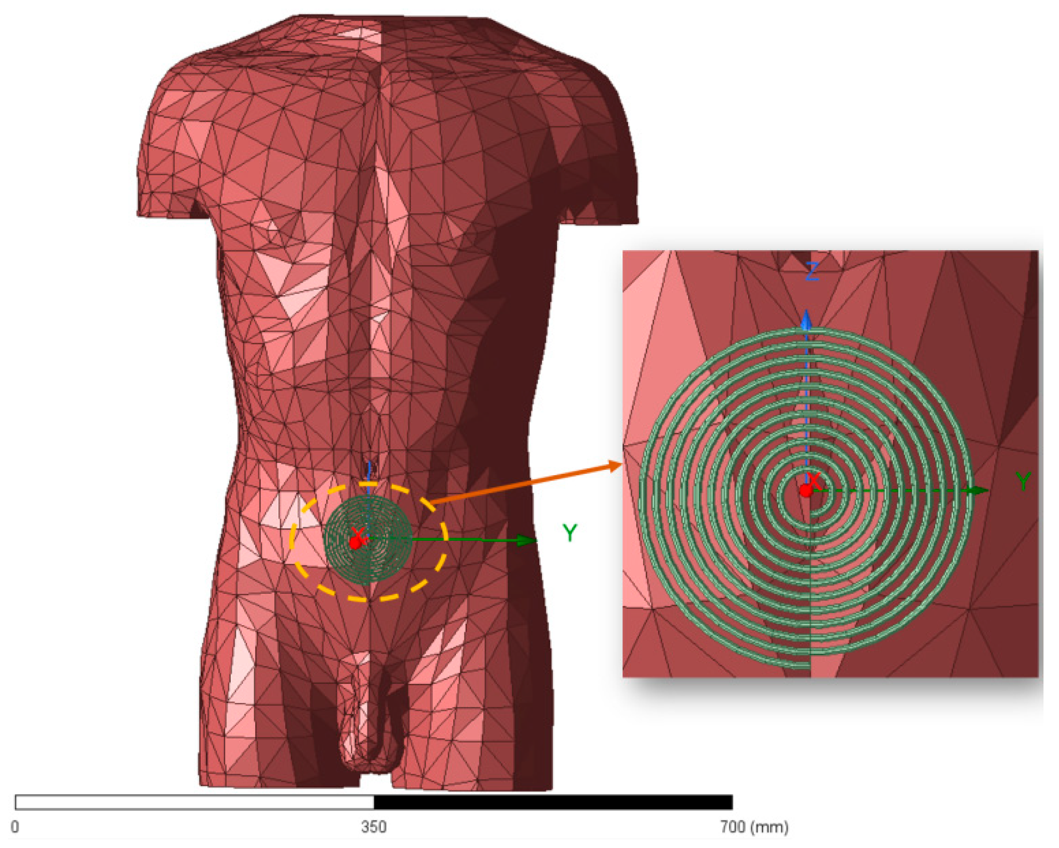
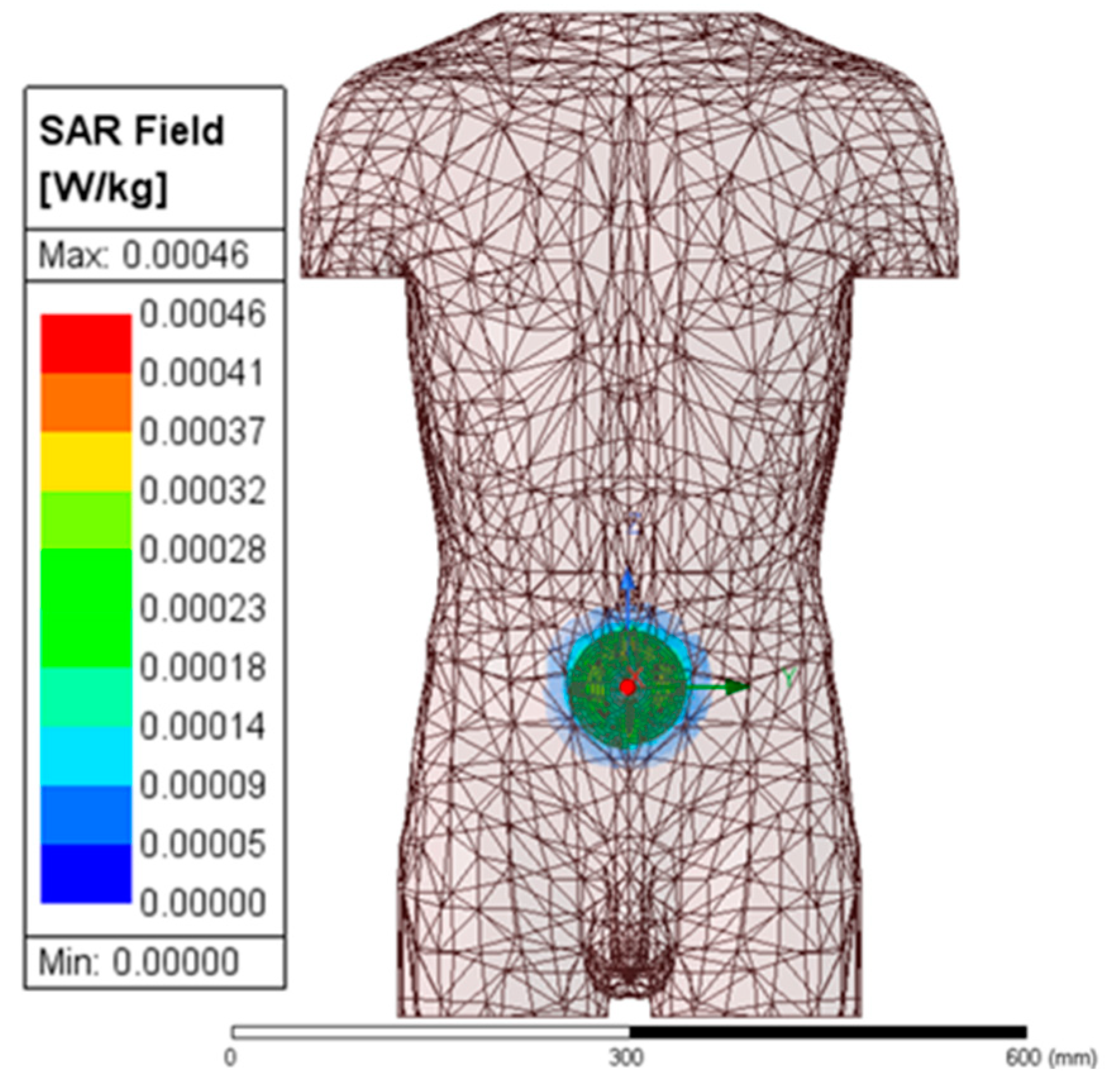
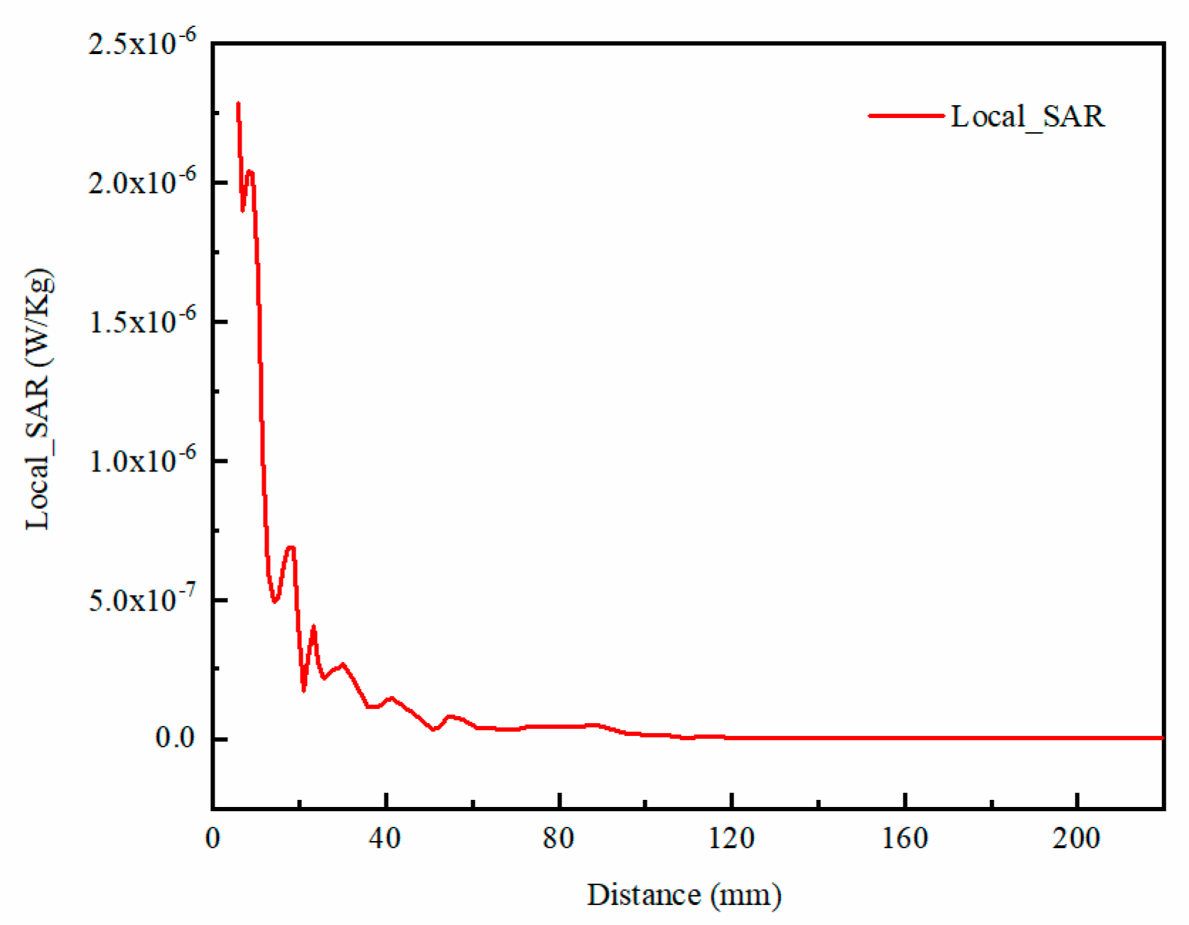
5.7. Verification of Electromagnetic Safety of Optimal Coil Structure
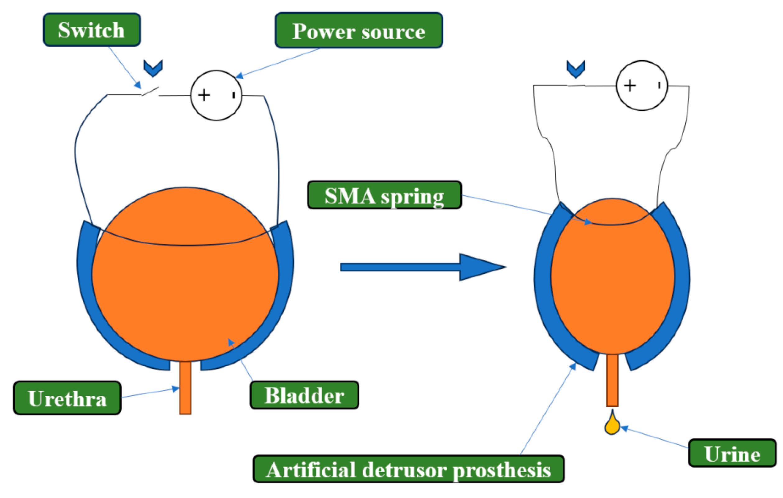
5.8. Analysis of the Performance Verification of Artificial Detrusor Powered by TET
6. Conclusions
Author Contributions
Funding
Data Availability Statement
Conflicts of Interest
References
- Wang, Z.F. Design of Ultra-Low Power SAR ADC for Implantable Medical Devices. Master’s Thesis, University of Electronic Science and Technology of China, Chengdu, China, 2015. [Google Scholar]
- Fumoto, H.; Shiose, A.; Flick, C.R.; Noble, L.D.; Duncan, B.W. Short-term in vivo performance of the cleveland clinic pedipump left ventricular assist device. Artif. Organs 2014, 38, 374–382. [Google Scholar] [PubMed]
- Cheng, S.M.; Jiang, P.P.; Wang, Y.B. Implantable electrical stimulation system for the treatment of functional gastrointestinal diseases and animal experimental study. Beijing Biomed. Eng. 2012, 31, 391–397. [Google Scholar]
- Lee, S.-Y.; Su, M.Y.; Liang, M.-C.; Chen, Y.-Y.; Hsieh, C.-H.; Yang, C.-M.; Lai, H.-Y.; Lin, J.-W.; Fang, Q. A programmable implantable microstimulator soc with wireless telemetry: Application in closed-loop endocardial stimulation for cardiac pacemaker. IEEE Trans. Biomed. Circuits Syst. 2011, 5, 511–522. [Google Scholar]
- Cho, S.H.; Xue, N.; Cauller, L.; Rosellini, W.; Lee, J.B. A su-8-based fully integrated biocompatible inductively powered wireless neurostimulator. J. Microelectromechanical Syst. 2013, 22, 170–176. [Google Scholar]
- Yu, Z.H. Photoresponsive Polymer Used as Artificial Retina to Restore Vision. Master’s Thesis, Nanjing University, Nanjing, China, 2021. [Google Scholar]
- Ke, L. Key Technology and Experimental Study of Feedback Artificial anal Sphincter System with Transcutaneous Energy Supply. Ph.D. Thesis, Shanghai Jiao Tong University, Shanghai, China, 2015. [Google Scholar]
- Wu, R.; Li, H.; Chen, J.; Le, Q.; Wang, L.; Huang, F.; Fu, Y. Design and optimization of coil for transcutaneous energy transmission system. Electronics 2024, 13, 2157. [Google Scholar] [CrossRef]
- Ke, L.; Yan, G.; Yan, S.; Wang, Z.; Li, X. Optimal design of litz wire coils with sandwich structure wirelessly powering an artificial anal sphincter system. Artif. Organs 2015, 39, 615–626. [Google Scholar] [CrossRef]
- Nithiyanandam, V.; Sampath, V. Approach-Based Analysis on Wireless Power Transmission for Bio-Implantable Devices. Appl. Sci. 2023, 13, 415. [Google Scholar]
- Khan, S.R.; Pavuluri, S.K.; Cummins, G.; Desmulliez, M.P.Y. Wireless power transfer techniques for implantable medical devices: A review. Sensors 2020, 20, 3487. [Google Scholar] [CrossRef]
- Zhang, Z.; Pang, H.; Georgiadis, A.; Cecati, C. Wireless power transfer—An overview. IEEE Trans. Ind. Electron. 2019, 66, 1044–1058. [Google Scholar]
- Shadid, R.; Noghanian, S. A literature survey on wireless power transfer for biomedical devices. Int. J. Antennas Propag. 2018, 2018, 4382841. [Google Scholar]
- Li, W.; Yuan, H.; Xu, W.; Geng, K.; Wang, G. An Optimization Procedure for Coil Design in a Dual Band Wireless Power and Data Transmission System. In Proceedings of the China Semiconductor Technology International Conference, Shanghai, China, 17–18 March 2013; Volume 52, pp. 1091–1097. [Google Scholar]
- Mutashar, S.; Hannan, M.A.; Samad, S.A.; Hussain, A. Analysis and Optimization of Spiral Circular Inductive Coupling Link for Bio-Implanted Applications on Air and within Human Tissue. Sensors 2014, 14, 11522–11541. [Google Scholar] [CrossRef]
- Jow, U.M.; Ghovanloo, M. Design and optimization of printed spiral coils for efficient transcutaneous inductive power transmission. IEEE Trans. Biomed. Circuits Syst. 2007, 1, 193–202. [Google Scholar] [CrossRef]
- Mutashar Abbas, S.; Hannan, M.A.; Samad, S.A.; Hussain, A. Design of spiral circular coils in wet and dry tissue for bio-implanted micro-system applications. Prog. Electromagn. Res. M 2013, 32, 181–200. [Google Scholar] [CrossRef]
- Kiani, M.; Jow, U.M.; Ghovanloo, M. Design and optimization of a 3-coil inductive link for efficient wireless power transmission. IEEE Trans. Biomed. Circuits Syst. 2011, 5, 579–591. [Google Scholar] [CrossRef]
- Kiani, M.; Ghovanloo, M. A figure-of-merit for designing high-performance inductive power transmission links. IEEE Trans. Ind. Electron. 2013, 60, 5292–5305. [Google Scholar] [CrossRef]
- Duan, Z.; Guo, Y.X.; Kwong, D.L. Rectangular coils optimization for wireless power transmission. Radio Sci. 2012, 47, 1–10. [Google Scholar] [CrossRef]
- Ben Fadhel, Y.; Ktata, S.; Sedraoui, K.; Rahmani, S.; Al-Haddad, K. A modified wireless power transfer system for medical implants. Energies 2019, 12, 1890. [Google Scholar] [CrossRef]
- Enssle, A.; Parspour, N.; Wu, F. Coil System Optimization for Transcutaneous Energy Transfer Systems. In Proceedings of the 2020 IEEE PELS Workshop on Emerging Technologies: Wireless Power Transfer (WoW), Seoul, Republic of Korea, 15–19 November 2020; IEEE: Piscataway, NJ, USA; pp. 141–145. [Google Scholar]
- Danilov, A.A.; Aubakirov, R.R.; Mindubaev, E.A.; Gurov, K.O.; Selishchev, S.V. An algorithm for the computer aided design of coil couple for a misalignment tolerant biomedical inductive powering unit. IEEE Access 2019, 7, 70755–70769. [Google Scholar] [CrossRef]
- Leung, H.Y.; Budgett, D.M.; Hu, A.P. Minimizing power loss in air-cored coils for tet heart pump systems. IEEE J. Emerg. Sel. Top. Circuits Syst. 2011, 1, 412–419. [Google Scholar] [CrossRef]
- Kim, J.; Basham, E.; Pedrotti, K.D. Geometry-based optimization of radio-frequency coils for powering neuroprosthetic implants. Med. Biol. Eng. Comput. 2013, 51, 123–134. [Google Scholar] [CrossRef]
- Liu, H.; Xu, Q.Q.; Yan, G.Z.; Li, H.W.; Yang, H.N. Design of Planar Spiral Coil in Transcutaneous Energy Transmission System. In Proceedings of the 11th World Congress on Intelligent Control and Automation (WCICA), Shenyang, China, 29 June–4 July 2014; pp. 2951–2955. [Google Scholar]
- Knecht, O.; Bosshard, R.; Kolar, J.W. High-Efficiency Transcutaneous Energy Transfer for Implantable Mechanical Heart Support Systems. IEEE Trans. ON Power Electron. 2015, 30, 6221–6236. [Google Scholar] [CrossRef]
- Gurov, K.O.; Mindubaev, E.A. Geometry Influence on the Coils Mutual Inductance in the Transcutaneous Energy Transfer System. In Proceedings of the 2018 IEEE Conference of Russian Young Researchers in Electrical and Electronic Engineering (EICONRUS), Moscow and St. Petersburg, Russia, 29 January–1 February 2018; pp. 1894–1896. [Google Scholar]
- Hua, F.F.; Yan, G.Z.; Wang, L.C. Optimization of transcutaneous wireless energy Supply for artificial anal sphincter system driven by dual-axis. Chin. J. Sci. Instrum. 2022, 43, 140–146. [Google Scholar]
- Qi, X.; Hao, W.; Zhao, L.G.; Zhi, H.M.; Ji, P.H.; Min, G.S. A Novel Mat-Based System for Position-Varying Wireless Power Transfer to Biomedical Implants. IEEE Trans. Magn. 2013, 49, 4774–4779. [Google Scholar]
- Rodrigues, G.A.; Lebensztajn, L. Study on transcutaneous energy transmission device optimal design. In Proceedings of the 2019 22nd International Conference on the Computation of Electromagnetic Fields (COMPUMAG), Paris, France, 15–19 July 2019; pp. 1–4. [Google Scholar]
- Liang, Y.B.; Hou, J.T.; Yang, X.U. Two-objective optimization design for the transcutaneous energy transmission system. Prz. Elektrotechniczny 2011, 87, 180–185. [Google Scholar]
- Ferreira, D.W.; Lebensztajn, L.; Krahenbuhl, L.; Morel, F.; Vollaire, C. A design proposal for optimal transcutaneous energy transmitters. IEEE Trans. Magn. 2014, 50, 997–1000. [Google Scholar] [CrossRef]
- Daniela, W.F.T.; Lebensztajn, L. Optimizing transcutaneous energy transmitter using game theory. IEEE Trans. Magn. 2016, 52, 8000904. [Google Scholar]
- Liu, X. Research on Characterization and Optimization of Power and Efficiency in Resonant Wireless Power Transfer System. Ph.D. Thesis, China University of Mining and Technology, Xuzhou, China, 2018. [Google Scholar]
- Huang, G.B.; Zhu, Q.Y.; Siew, C.K. Extreme learning machine: Theory and applications. Neurocomputing 2006, 70, 489–501. [Google Scholar] [CrossRef]
- Zhang, Q.; Lu, J.; Jin, Y. Artificial intelligence in recommender systems. Complex Intell. Syst. 2021, 7, 439–457. [Google Scholar] [CrossRef]
- Bacanin, N.; Tuba, E.; Zivkovic, M.; Strumberger, I.; Tuba, M. Whale optimization algorithm with exploratory move for wireless sensor networks localization. Int. Conf. Hybrid Intell. Syst. 2019, 328–338. [Google Scholar] [CrossRef]
- Zivkovic, M.; Bacanin, N.; Venkatachalam, K.; Nayyar, A.; Djordjevic, A.; Strumberger, I.; Al-Turjman, F. COVID-19 cases prediction by using hybrid machine learning and beetle antennae search approach. Sustain. Cities Soc. 2021, 66, 102669. [Google Scholar] [CrossRef]
- Salb, M.; Zivkovic, M.; Bacanin, N.; Chhabra, A.; Suresh, M. Support vector machine performance improvements for cryptocurrency value forecasting by enhanced sine cosine algorithm. Comput. Vis. Robot. 2022, 527–536. [Google Scholar] [CrossRef]
- AlHosni, N.; Jovanovic, L.; Antonijevic, M.; Bukumira, M.; Zivkovic, M.; Strumberger, I.; Mani, J.P.; Bacanin, N. The Xgboost model for network intrusion detection boosted by enhanced sine cosine algorithm. In International Conference on Image Processing and Capsule Networks; Springer International Publishing: Cham, Switzerland, 2022; pp. 213–228. [Google Scholar]
- Tair, M.; Bacanin, N.; Zivkovic, M.; Venkatachalam, K.; Strumberger, I. Xgboost design by multi-verse optimiser: An application for network intrusion detection. Mob. Comput. Sustain. Inform. 2022, 1–16. [Google Scholar] [CrossRef]
- Zivkovic, M.; Bacanin, N.; Arandjelovic, J.; Rakic, A.; Strumberger, I.; Venkatachalam, K.; Joseph, P.M. Novel harris hawks optimization and deep neural network approach for intrusion detection. In Proceedings of International Joint Conference on Advances in Computational Intelligence; Algorithms for Intelligent Systems; Uddin, M.S., Jamwal, P.K., Bansal, J.C., Eds.; Springer: Singapore, 2022; pp. 239–250. [Google Scholar] [CrossRef]
- Bezdan, T.; Zivkovic, M.; Bacanin, N.; Chhabra, A.; Suresh, M. Feature selection by hybrid brain storm optimization algorithm for COVID-19 classification. J. Comput. Biol. 2022, 29, 515–529. [Google Scholar]
- Budimirovic, N.; Prabhu, E.; Antonijevic, M.; Zivkovic, M.; Bacanin, N.; Strumberger, I.; Venkatachalam, K. COVID-19 severity prediction using enhanced whale with salp swarm feature classification. Comput. Mater. Contin. 2022, 72, 1685–1698. [Google Scholar]
- Strumberger, I.; Rakic, A.; Stanojlovic, S.; Arandjelovic, J.; Bezdan, T.; Zivkovic, M.; Bacanin, N. Feature selection by hybrid binary ant lion optimizer with COVID-19 dataset. In Proceedings of the 2021 29th Telecommunications Forum (TELFOR), Belgrade, Serbia, 23–24 November 2021. [Google Scholar]
- Zivkovic, M.; Petrovic, A.; Bacanin, N.; Milosevic, S.; Veljic, V.; Vesic, A. The COVID-19 images classification by mobilenetv3 and enhanced sine cosine metaheuristics. Mob. Comput. Sustain. Inform. 2022, 937–950. [Google Scholar] [CrossRef]
- Bezdan, T.; Zivkovic, M.; Tuba, E.; Strumberger, I.; Bacanin, N.; Tuba, M. Glioma brain tumor grade classification from mri using convolutional neural networks designed by modified fa. In Intelligent and Fuzzy Techniques: Smart and Innovative Solutions. INFUS 2020. Advances in Intelligent Systems and Computing; Kahraman, C., Cevik Onar, S., Oztaysi, B., Sari, I., Cebi, S., Tolga, A., Eds.; Springer: Cham, Switzerland, 2020; Volume 1197. [Google Scholar] [CrossRef]
- Bacanin, N.; Stoean, C.; Markovic, D. Improving performance of extreme learning machine for classification challenges by modified firefly algorithm and validation on medical benchmark datasets. Multimedia Tools Appl. 2024, 83, 76035–76075. [Google Scholar]
- Bacanin, N.; Zivkovic, M.; Antonijevic, M. Addressing feature selection and extreme learning machine tuning by diversity-oriented social network search: An application for phishing websites detection. Complex Intell. Syst. 2023, 9, 7269–7304. [Google Scholar]
- Van Thieu, N.; Nguyen, N.H.; Sherif, M.; El-Shafie, A.; Ahmed, A.N. Integrated metaheuristic algorithms with extreme learning machine models for river streamflow prediction. Sci. Rep. 2024, 14, 13597. [Google Scholar]
- Adnan, R.M.; Dai, H.-L.; Mostafa, R.R.; Islam, A.R.M.T.; Kisi, O.; Heddam, S.; Zounemat-Kermani, M. Modelling groundwater level fluctuations by ELM merged advanced metaheuristic algorithms using hydroclimatic data. Geocarto Int. 2022, 38, 2158951. [Google Scholar]
- Bacanin, N.; Stoean, C.; Zivkovic, M.; Jovanovic, D.; Antonijevic, M.; Mladenovic, D. Multi-swarm algorithm for extreme learning machine optimization. Sensors 2022, 22, 4204. [Google Scholar] [CrossRef]
- Bui, D.T.; Ngo, P.-T.T.; Pham, T.D.; Jaafari, A.; Minh, N.Q.; Hoa, P.V.; Samui, P. A novel hybrid approach based on a swarm intelligence optimized extreme learning machine for flash flood susceptibility mapping. Catena 2019, 179, 184–196. [Google Scholar]
- Alshamiri, A.K.; Singh, A.; Surampudi, B.R. Two swarm intelligence approaches for tuning extreme learning machine. Int. J. Mach. Learn. Cybern. 2018, 9, 1271–1283. [Google Scholar]
- Wolpert, D.H.; Macready, W.G. No free lunch theorems for optimization. IEEE Trans. Evol. Comput. 1997, 1, 67–82. [Google Scholar] [CrossRef]
- Mirjalili, S.; Mirjalili, S.M.; Lewis, A. Grey wolf optimizer. Adv. Eng. Softw. 2014, 69, 46–61. [Google Scholar]
- Jangir, P.; Jangir, N. Non-dominated sorting whale optimization algorithm (NSWOA): A multi-objective optimization algorithm for solving engineering design problems. Glob. J. Res. Eng. 2017, 17, 15–42. [Google Scholar]
- Zhang, W.; Mi, C.C. Compensation topologies of high-power wireless power transfer systems. IEEE Trans. Veh. Technol. 2016, 65, 4768–4778. [Google Scholar]
- Yang, H.J. Parameter Programming and Constant current/Constant Voltage Research of Magnetic Coupling Wireless Power Transfer System Based on LCC-S Topological Structure. Master’s Thesis, Chongqing University of Technology, Chongqing, China, 2022. [Google Scholar]
- Kritikos, H.N.; Foster, K.R.; Schwan, H.P. Temperature profiles in spheres due to electromagnetic heating. J. Microw. Power 1981, 16, 327–344. [Google Scholar]
- Djuric, N.; Gavrilov, T.; Kljajic, D. The ICNIRP 2020 Guidelines and Serbian EMF Legislation. In Proceedings of the 29th Telecommunications Forum (TELFOR), Belgrade, Serbia, 23–24 November 2021. [Google Scholar]
- Repacholi, M.H.; Grandolfo, M.; Ahlbom, A.; Bergqvist, U.; Matthes, R. Health issues related to the use of hand-held radiotelephones and base transmitters. Health Phys. 1996, 70, 587–593. [Google Scholar]
- Zhang, S.X.; Heng, P.A.; Liu, Z.J. Chinese visible human project. Clin. Anat. Off. J. Am. Assoc. Clin. Anat. Br. Assoc. Clin. Anat. 2006, 19, 204–215. [Google Scholar]


| Type | |||
|---|---|---|---|
| Parameter | |||
| SS | |||
| SP | |||
| PS | |||
| PP | |||
| Result Category | Measurement Parameters | ||
|---|---|---|---|
| (mΩ) | (uH) | ||
| Simulation | 34.52 | 15.24 | 27.7 |
| Experiment | 37.2 | 16.22 | 27.4 |
| Simulation error | 7.2% | 6% | 1.1% |
| Algorithm | Parameter | Value |
|---|---|---|
| PSO | 1.2 1.5 0.7 | |
| DE | [0.2, 0.8] 0.2 | |
| GWO | [0, 1] [0, 1] | |
| HOACFOA | [0, 50] [0, 1] |
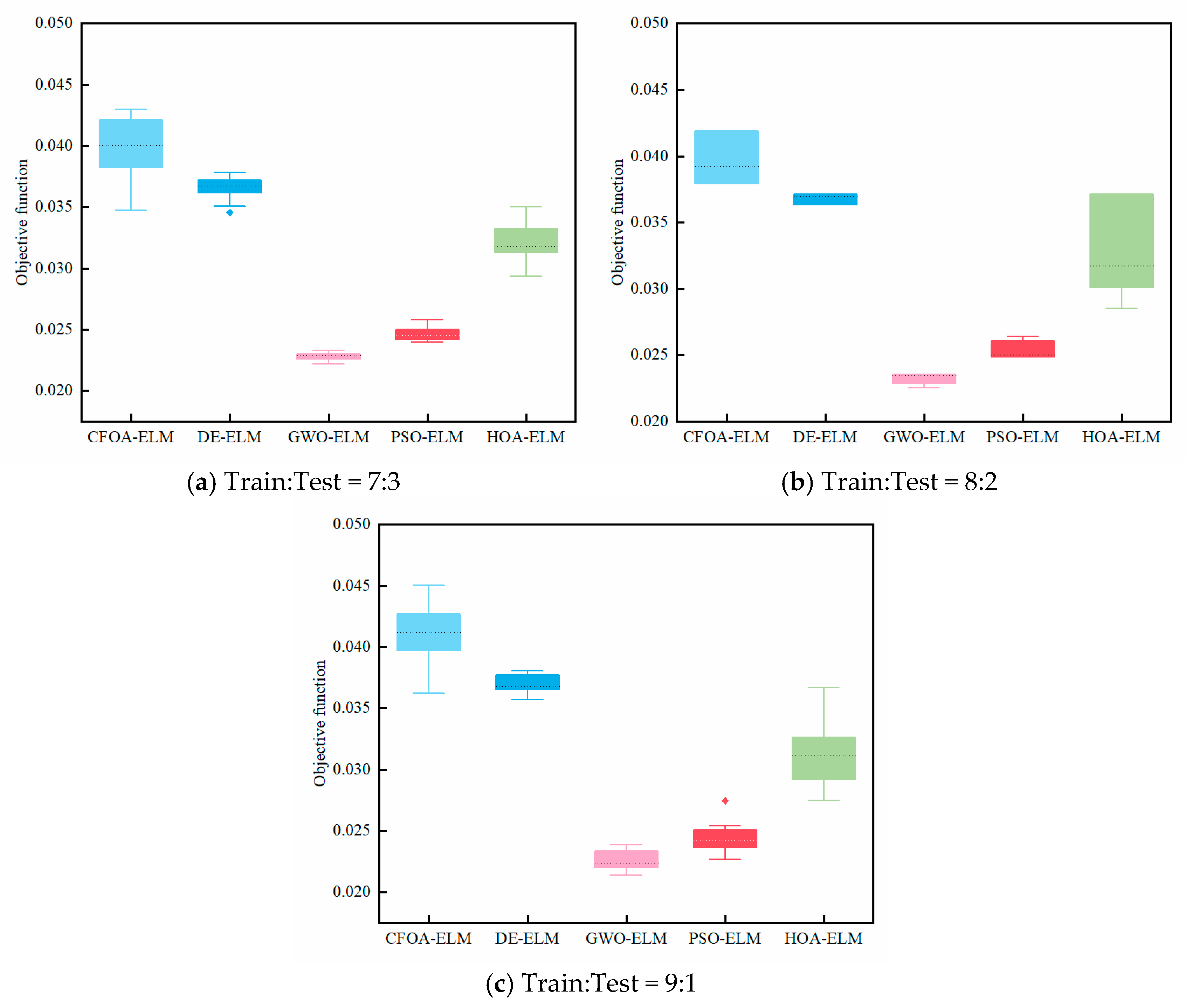
| Train: Test | Metrics | CFOA-ELM | DE-ELM | GWO-ELM | PSO-ELM | HOA-ELM |
|---|---|---|---|---|---|---|
| 7:3 | Best | 3.47 × 10⁻² | 3.45 × 10⁻² | 2.22 × 10⁻² | 2.40 × 10⁻² | 2.94 × 10⁻² |
| Worst | 4.30 × 10⁻² | 3.78 × 10⁻² | 2.33 × 10⁻² | 2.58 × 10⁻² | 3.50 × 10⁻² | |
| Mean | 3.97 × 10⁻² | 3.66 × 10⁻² | 2.28 × 10⁻² | 2.47 × 10⁻² | 3.21 × 10⁻² | |
| Median | 4.01 × 10⁻² | 3.68 × 10⁻² | 2.29 × 10⁻² | 2.46 × 10⁻² | 3.18 × 10⁻² | |
| Std | 2.48 × 10⁻³ | 1.01 × 10⁻³ | 3.36 × 10⁻⁴ | 5.19 × 10⁻⁴ | 1.31 × 10⁻³ | |
| Var | 6.16 × 10⁻⁶ | 1.01 × 10⁻⁶ | 1.13 × 10⁻⁷ | 2.69 × 10⁻⁷ | 1.72 × 10⁻⁶ | |
| 8:2 | Best | 3.79 × 10⁻² | 3.64 × 10⁻² | 2.26 × 10⁻² | 2.49 × 10⁻² | 2.85 × 10⁻² |
| Worst | 4.19 × 10⁻² | 3.71 × 10⁻² | 2.35 × 10⁻² | 2.64 × 10⁻² | 3.71 × 10⁻² | |
| Mean | 3.98 × 10⁻² | 3.68 × 10⁻² | 2.33 × 10⁻² | 2.53 × 10⁻² | 3.24 × 10⁻² | |
| Median | 3.93 × 10⁻² | 3.69 × 10⁻² | 2.35 × 10⁻² | 2.50 × 10⁻² | 3.17 × 10⁻² | |
| Std | 1.71 × 10⁻³ | 3.25 × 10⁻⁴ | 3.35 × 10⁻⁴ | 5.64 × 10⁻⁴ | 2.99 × 10⁻³ | |
| Var | 2.94 × 10⁻⁶ | 1.06 × 10⁻⁷ | 1.12 × 10⁻⁷ | 3.18 × 10⁻⁷ | 8.93 × 10⁻⁶ | |
| 9:1 | Best | 3.62 × 10⁻² | 3.57 × 10⁻² | 2.14 × 10⁻² | 2.26 × 10⁻² | 2.75 × 10⁻² |
| Worst | 4.50 × 10⁻² | 3.81 × 10⁻² | 2.39 × 10⁻² | 2.75 × 10⁻² | 3.67 × 10⁻² | |
| Mean | 4.10 × 10⁻² | 3.69 × 10⁻² | 2.26 × 10⁻² | 2.44 × 10⁻² | 3.12 × 10⁻² | |
| Median | 4.12 × 10⁻² | 3.68 × 10⁻² | 2.23 × 10⁻² | 2.42 × 10⁻² | 3.12 × 10⁻² | |
| Std | 2.38 × 10⁻³ | 6.69 × 10⁻⁴ | 6.85 × 10⁻⁴ | 1.09 × 10⁻³ | 2.28 × 10⁻³ | |
| Var | 5.68 × 10⁻⁶ | 4.48 × 10⁻⁷ | 4.69 × 10⁻⁷ | 1.19 × 10⁻⁶ | 5.20 × 10⁻⁶ |
| Train: Test | GWO-ELM vs. CFOA-ELM | GWO-ELM vs. DE-ELM | GWO-ELM vs. PSO-ELM | GWO-ELM vs. HOA-ELM |
|---|---|---|---|---|
| 7:3 | 3.05 × 10⁻⁵ | 3.05 × 10⁻⁵ | 3.05 × 10⁻⁵ | 3.05 × 10⁻⁵ |
| 8:2 | 3.05 × 10⁻⁵ | 3.05 × 10⁻⁵ | 3.05 × 10⁻⁵ | 3.05 × 10⁻⁵ |
| 9:1 | 3.05 × 10⁻⁵ | 3.05 × 10⁻⁵ | 1.53 × 10⁻⁴ | 3.05 × 10⁻⁵ |
| Output | Metrics | CFOA | DE-ELM | GWO-ELM | PSO-ELM | HOA-ELM | ELM |
|---|---|---|---|---|---|---|---|
| -ELM | |||||||
| 5.00 × 10⁻² | 4.90 × 10⁻² | 2.72 × 10⁻² | 2.94 × 10⁻² | 3.49 × 10⁻² | 8.66 × 10⁻² | ||
| 9.40 × 10⁻¹ | 9.39 × 10⁻¹ | 9.83 × 10⁻¹ | 9.79 × 10⁻¹ | 9.70 × 10⁻¹ | 8.25 × 10⁻¹ | ||
| 3.88 × 10⁻² | 3.71 × 10⁻² | 1.96 × 10⁻² | 2.21 × 10⁻² | 2.63 × 10⁻² | 6.53 × 10⁻² | ||
| 5.12 × 10⁻¹ | 5.98 × 10⁻¹ | 1.82 × 10⁻¹ | 3.64 × 10⁻¹ | 6.67 × 10⁻¹ | 2.13 | ||
| 0.99978 | 0.99970 | 0.99997 | 0.99989 | 0.99963 | 0.99620 | ||
| 3.84 × 10⁻¹ | 4.32 × 10⁻¹ | 1.36 × 10⁻¹ | 2.56 × 10⁻¹ | 4.82 × 10⁻¹ | 1.58 | ||
| 2.78 × 10⁻² | 2.85 × 10⁻² | 2.16 × 10⁻² | 2.28 × 10⁻² | 2.69 × 10⁻² | 3.04 × 10⁻² | ||
| 9.61 × 10⁻¹ | 9.60 × 10⁻¹ | 9.78 × 10⁻¹ | 9.75 × 10⁻¹ | 9.64 × 10⁻¹ | 9.53 × 10⁻¹ | ||
| 2.14 × 10⁻² | 2.20 × 10⁻² | 1.60 × 10⁻² | 1.67 × 10⁻² | 1.92 × 10⁻² | 2.31 × 10⁻² |
| Output | Metrics | CFOA | DE-ELM | GWO-ELM | PSO-ELM | HOA-ELM | ELM |
|---|---|---|---|---|---|---|---|
| -ELM | |||||||
| 5.64 × 10⁻² | 4.61 × 10⁻² | 2.82 × 10⁻² | 3.13 × 10⁻² | 3.80 × 10⁻² | 7.63 × 10⁻² | ||
| 9.23 × 10⁻¹ | 9.48 × 10⁻¹ | 9.81 × 10⁻¹ | 9.76 × 10⁻¹ | 9.63 × 10⁻¹ | 8.65 × 10⁻¹ | ||
| 4.43 × 10⁻² | 3.59 × 10⁻² | 2.00 × 10⁻² | 2.35 × 10⁻² | 2.81 × 10⁻² | 6.19 × 10⁻² | ||
| 1.15 | 1.35 | 1.27 × 10⁻¹ | 2.58 × 10⁻¹ | 4.27 × 10⁻¹ | 1.65 | ||
| 0.9988 | 0.99847 | 0.99999 | 0.99994 | 0.99985 | 0.9977 | ||
| 8.20 × 10⁻¹ | 9.87 × 10⁻¹ | 9.94 × 10⁻² | 2.01 × 10⁻¹ | 3.14 × 10⁻¹ | 1.23 | ||
| 2.75 × 10⁻² | 2.95 × 10⁻² | 2.18 × 10⁻² | 2.34 × 10⁻² | 2.56 × 10⁻² | 4.41 × 10⁻² | ||
| 9.61 × 10⁻¹ | 9.54 × 10⁻¹ | 9.77 × 10⁻¹ | 9.73 × 10⁻¹ | 9.67 × 10⁻¹ | 9.06 × 10⁻¹ | ||
| 2.08 × 10⁻² | 2.25 × 10⁻² | 1.67 × 10⁻² | 1.71 × 10⁻² | 1.99 × 10⁻² | 3.49 × 10⁻² |
| Output | Metrics | CFOA | DE-ELM | GWO-ELM | PSO-ELM | HOA-ELM | ELM |
|---|---|---|---|---|---|---|---|
| -ELM | |||||||
| 5.42 × 10⁻² | 4.91 × 10⁻² | 2.46 × 10⁻² | 2.97 × 10⁻² | 3.10 × 10⁻² | 7.66 × 10⁻² | ||
| 9.22 × 10⁻¹ | 9.33 × 10⁻¹ | 9.83 × 10⁻¹ | 9.74 × 10⁻¹ | 9.72 × 10⁻¹ | 8.51 × 10⁻¹ | ||
| 4.20 × 10⁻² | 3.82 × 10⁻² | 1.73 × 10⁻² | 2.26 × 10⁻² | 2.33 × 10⁻² | 6.14 × 10⁻² | ||
| k | 9.82 × 10⁻¹ | 6.87 × 10⁻¹ | 1.18 × 10⁻¹ | 2.07 × 10⁻¹ | 4.29 × 10⁻¹ | 1.60 | |
| 0.99919 | 0.99961 | 0.99999 | 0.99996 | 0.99985 | 0.9978 | ||
| 7.11 × 10⁻¹ | 5.03 × 10⁻¹ | 9.34 × 10⁻² | 1.54 × 10⁻¹ | 3.10 × 10⁻¹ | 1.14 | ||
| 2.58 × 10⁻² | 2.84 × 10⁻² | 2.04 × 10⁻² | 1.92 × 10⁻² | 2.54 × 10⁻² | 5.10 × 10⁻² | ||
| 9.65 × 10⁻¹ | 9.59 × 10⁻¹ | 9.80 × 10⁻¹ | 9.81 × 10⁻¹ | 9.67 × 10⁻¹ | 8.69 × 10⁻¹ | ||
| 1.98 × 10⁻² | 2.13 × 10⁻² | 1.53 × 10⁻² | 1.43 × 10⁻² | 1.92 × 10⁻² | 3.95 × 10⁻² |
| Metrics | Algorithm | |||||
|---|---|---|---|---|---|---|
| MOPSO | MOMVO | NSWOA | MSSA | MODA | ||
| IGD | Best | 5.94 × 10⁻¹ | 8.57 × 10⁻¹ | 3.90 × 10⁻¹ | 1.20 | 1.50 |
| Worst | 1.42 | 4.70 | 5.84 × 10⁻¹ | 5.52 | 4.92 | |
| Mean | 1.00 | 1.86 | 4.59 × 10⁻¹ | 2.73 | 2.40 | |
| Median | 9.91 × 10⁻¹ | 1.47 | 4.56 × 10⁻¹ | 2.27 | 2.47 | |
| Std | 1.85 × 10⁻¹ | 1.13 | 4.51 × 10⁻² | 1.37 | 8.63 × 10⁻¹ | |
| Var | 3.42 × 10⁻² | 1.27 | 2.04 × 10⁻³ | 1.87 | 7.45 × 10⁻¹ | |
| HV | Best | 5.92 × 10⁻¹ | 6.91 × 10⁻¹ | 5.97 × 10⁻¹ | 6.91 × 10⁻¹ | 6.71 × 10⁻¹ |
| Worst | 5.79 × 10⁻¹ | 5.48 × 10⁻¹ | 5.92 × 10⁻¹ | 5.12 × 10⁻¹ | 5.48 × 10⁻¹ | |
| Mean | 5.85 × 10⁻¹ | 6.11 × 10⁻¹ | 5.95 × 10⁻¹ | 5.89 × 10⁻¹ | 5.76 × 10⁻¹ | |
| Median | 5.87 × 10⁻¹ | 5.99 × 10⁻¹ | 5.96 × 10⁻¹ | 5.78 × 10⁻¹ | 5.69 × 10⁻¹ | |
| Std | 4.31 × 10⁻³ | 4.22 × 10⁻² | 1.60 × 10⁻³ | 4.02 × 10⁻² | 2.80 × 10⁻² | |
| Var | 1.86 × 10⁻⁵ | 1.78 × 10⁻³ | 2.57 × 10⁻⁶ | 1.61 × 10⁻³ | 7.82 × 10⁻⁴ | |
| SP | Best | 9.24 × 10⁻¹ | 8.59 × 10⁻¹ | 6.84 × 10⁻¹ | 9.19 × 10⁻¹ | 6.43 × 10⁻¹ |
| Worst | 1.60 | 2.47 | 9.05 × 10⁻¹ | 4.55 | 6.21 | |
| Mean | 1.17 | 1.54 | 7.83 × 10⁻¹ | 2.00 | 2.94 | |
| Median | 1.12 | 1.55 | 7.97 × 10⁻¹ | 1.51 | 3.00 | |
| Std | 1.73 × 10⁻¹ | 4.47 × 10⁻¹ | 6.90 × 10⁻² | 1.11 | 1.29 | |
| Var | 3.00 × 10⁻² | 1.99 × 10⁻¹ | 4.77 × 10⁻³ | 1.23 | 1.67 | |
| Spread | Best | 9.03 × 10⁻¹ | 1.07 | 6.45 × 10⁻¹ | 1.18 | 1.35 |
| Worst | 1.14 | 1.32 | 8.48 × 10⁻¹ | 1.68 | 1.85 | |
| Mean | 1.04 | 1.22 | 7.41 × 10⁻¹ | 1.43 | 1.68 | |
| Median | 1.03 | 1.25 | 7.29 × 10⁻¹ | 1.43 | 1.73 | |
| Std | 6.38 × 10⁻² | 7.77 × 10⁻² | 5.66 × 10⁻² | 1.52 × 10⁻¹ | 1.29 × 10⁻¹ | |
| Var | 4.07 × 10⁻³ | 6.04 × 10⁻³ | 3.21 × 10⁻³ | 2.32 × 10⁻² | 1.66 × 10⁻² | |
| Metrics | NSWOA vs. MOPSO | NSWOA vs. MOMVO | NSWOA vs. MSSA | NSWOA vs. MODA |
|---|---|---|---|---|
| IGD | 3.05 × 10⁻⁵ | 3.05 × 10⁻⁵ | 3.05 × 10⁻⁵ | 3.05 × 10⁻⁵ |
| HV | 3.05 × 10⁻⁵ | 8.2 × 10⁻¹ | 1.4 × 10⁻¹ | 4.18 × 10⁻³ |
| SP | 3.05 × 10⁻⁵ | 3.05 × 10⁻⁵ | 3.05 × 10⁻⁵ | 6.10 × 10⁻⁵ |
| Spread | 3.05 × 10⁻⁵ | 3.05 × 10⁻⁵ | 3.05 × 10⁻⁵ | 3.05 × 10⁻⁵ |
| Candidate Solution | Decision Variables | Optimization Objective | ||||||
|---|---|---|---|---|---|---|---|---|
| (mm) | (mm) | (kHz) | (mm) | |||||
| 1 | 5.00 | 5.00 | 1.66 | 0.00 | 341.53 | 0.54 | 0.09 | 17.50 |
| 2 | 25.56 | 15.46 | 0.09 | 1.79 | 129.56 | 1.00 | 0.44 | 90.45 |
| 3 | 31.00 | 25.00 | 0.15 | 2.00 | 400.00 | 0.95 | 0.60 | 154.07 |
| 4 | 10.63 | 21.42 | 1.62 | 0.00 | 281.05 | 0.99 | 0.29 | 50.85 |
| Parameters | Explanation | Values |
|---|---|---|
| Inductance of the primary coil | 4.143 × 10⁻⁶ H | |
| Inductance of the secondary coil | 10.394 × 10⁻⁶ H | |
| Inductance of LCC-S topology component | 1.6 × 10⁻⁶ H | |
| (LCC-S) | LCC-S topology primary tuning capacitor | 1.26 × 10⁻⁷ F |
| (S-S) | S-S topology primary tuning capacitor | 7.74 × 10⁻⁸ F |
| (LCC-S) | LCC-S topology secondary tuning capacitor | 2.93 × 10⁻⁸ F |
| (S-S) | S-S topology secondary tuning capacitor | 2.93 × 10⁻⁸ F |
| tuning capacitor | 2 × 10⁻⁷ F | |
| Mutual inductance of coils | 1 × 10⁻⁶ H~1.95 × 10⁻⁶ H | |
| Primary coil resistance | 34 mΩ | |
| Secondary coil resistance | 156 mΩ | |
| Filter capacitor | 4.7 × 10⁻⁶ F | |
| Load resistance | 5 Ω | |
| DC voltage source | 15 V |
Disclaimer/Publisher’s Note: The statements, opinions and data contained in all publications are solely those of the individual author(s) and contributor(s) and not of MDPI and/or the editor(s). MDPI and/or the editor(s) disclaim responsibility for any injury to people or property resulting from any ideas, methods, instructions or products referred to in the content. |
© 2025 by the authors. Licensee MDPI, Basel, Switzerland. This article is an open access article distributed under the terms and conditions of the Creative Commons Attribution (CC BY) license (https://creativecommons.org/licenses/by/4.0/).
Share and Cite
Yin, M.; Li, X. Modeling and Multi-Objective Optimization of Transcutaneous Energy Transmission Coils Based on Artificial Intelligence. Electronics 2025, 14, 1381. https://doi.org/10.3390/electronics14071381
Yin M, Li X. Modeling and Multi-Objective Optimization of Transcutaneous Energy Transmission Coils Based on Artificial Intelligence. Electronics. 2025; 14(7):1381. https://doi.org/10.3390/electronics14071381
Chicago/Turabian StyleYin, Mao, and Xiao Li. 2025. "Modeling and Multi-Objective Optimization of Transcutaneous Energy Transmission Coils Based on Artificial Intelligence" Electronics 14, no. 7: 1381. https://doi.org/10.3390/electronics14071381
APA StyleYin, M., & Li, X. (2025). Modeling and Multi-Objective Optimization of Transcutaneous Energy Transmission Coils Based on Artificial Intelligence. Electronics, 14(7), 1381. https://doi.org/10.3390/electronics14071381