Analyzing the Effect of Error Estimation on Random Missing Data Patterns in Mid-Term Electrical Forecasting

Abstract

In smart buildings, time series forecasting of electrical load is essential for energy optimization, demand response, and overall building performance. However, the mid-term load forecasting (MTLF) can be particularly challenging due to several uncertainties, such as sensor malfunctions, communication failures, and external environmental factors. These problems can lead to missing data patterns that may impact the accuracy and reliability of forecasting models. The purpose of this study is to explore the impact of random missing data patterns on the MTLF predictions’ accuracy. Therefore, several data imputation techniques are evaluated using a complete dataset (i.e., with no missing values) acquired on a smart commercial building, and their influence on load forecasting performance is assessed when different percentages of randomly distributed missing data patterns are assumed. Moreover, the deep learning (DL) approach based on a recurrent neural network, namely, long short-term memory (LSTM), is employed to predict the smart building electrical energy consumption. The obtained outcomes demonstrate that the pattern of random missing data significantly impacts the forecasting accuracy, with machine learning (ML) imputation techniques having better results than statistical and hybrid imputation techniques. Based on these findings, it is evident that robust data preprocessing and the handling of missing values are important in order to improve the accuracy and reliability of mid-term electrical load forecasts.

1. Introduction

The accurate prediction of electrical loads is essential for the effective management of power systems since it enables utilities to strategically plan and enhance energy production, distribution, and infrastructure investments. Mid-term load forecasting (MTLF) models, usually ranging from days to weeks and extending up to months, are particularly important for the planning of power systems, tariff setting, and energy trading activities [1]. However, the precision of forecasting models is frequently affected by missing data, which may be caused by from sensor malfunctions, data transmission issues, or incomplete records. The missing data introduce uncertainty and compromise the reliability of forecasting models, making it essential to apply robust error estimation and imputation methods [2].

Accurate MTLF is mainly dependent on data quality, and the performance of the model can be significantly jeopardized by the presence of missing values. Therefore, it is necessary to investigate methods to avoid such insufficiencies in data analysis. In order to formulate a comprehensive strategy for determining the optimal approach to manage missing values, it is essential to understand the fundamental factors that lead to their appearance. Missing data are conventionally categorized into three distinct types of errors [3], which are specified as follows:

• Missing completely at random (MCAR): This indicates that both observed and unobserved variables have no impact on the missingness of data. Although the MCAR assumption is important in that it allows for the obtaining of unbiased estimation regardless of missing values, it is not feasible in many real-world data scenarios [4]. Statistically, the MCAR mechanism can be expressed as:

  $$f(Y\mid X,\theta )=f(Y\mid \theta ) \mathrm{for} \mathrm{all} X,\theta$$

  (1)
  In Equation (1), X and Y denote a vector of observed data values and a vector of missingness indicators, respectively; $\theta$ is an unknown parameter; and the function f denotes the conditional probability distribution.
• Missing at random (MAR): Missingness is associated with observed but not unobserved variables. A dataset that is consistent with the MAR assumption may or may not result in a biased estimate.

  $$f(Y\mid X,\theta )=f(Y\mid X_{\mathrm{obs}},\theta )\mathrm{for}\mathrm{all}{X}_{\mathrm{mis}},\theta$$

  (2)
  In Equation (3), $X_{\mathrm{obs}}$ and $X_{\mathrm{mis}}$ are the observed and missing components of the target variable X. The unknown parameter $\theta$ can be estimated by relating $X_{\mathrm{obs}}$ with other explanatory variables [5].
• Missing not at random (MNAR): The occurrence of missingness is linked to unobserved variables, i.e., missing values come from unmeasured events or unidentified factors. A dataset with the MNAR assumption may or may not produce a biased estimate, much like MAR data [6]. Mathematically, MNAR can be expressed as shown in Equation (3):

  $$f(Y,X\mid \lambda ,\theta )=f(Y\mid \lambda )f(Y\mid X,\theta )$$

  (3)

  where $\lambda$ is a parameter of the distribution of X that is estimated from the observed data, and $\theta$ is a parameter that characterizes the distribution of the missingness pattern.

Randomly missing data, especially the MAR, can lead to changes in patterns and to the lower accuracy of predictive models [7]. Therefore, effective imputation methods need to be applied in order to reduce the impact of missing data on the forecasting model to make them robust.

Missing data can be preprocessed through several statistical methods such as substitution techniques or regression-based imputation methods. Substitution-based methods are simple and computationally efficient (e.g., mean, median, and mode) but can underestimate variance and distort the relationships among variables, and these techniques are not able to capture complex dependencies in the time series data [8]. However, regression-based imputation methods utilize the inter-variable correlations to predict and fill the gaps in the data. These techniques utilize existing data from other variables to develop a regression model (e.g., linear or multiple regression) that estimates missing values by examining the basic patterns evident within the dataset. Regression imputation makes it possible to recover these relationships by using predictors that have strong correlations with the variable being imputed, which tends to result in more accurate imputation compared to a simple substitution [9].

On the other hand, imputation methods based on machine learning (ML) and more complex DL models provide more advanced solutions by using both time dependencies and underlying structures in the data [10]. Recent studies suggest that, for various missing data patterns, ML-based imputation strategies are more accurate than the traditional statistical methods when the forecasting accuracy is considered [11]. Furthermore, they provide enhanced capability in identifying complex patterns, which makes them particularly effective in high-dimensional and dynamic datasets.

The hybrid imputation methodology, which combines both traditional statistical techniques and ML algorithms, provides a more effective approach in dealing with missing data, especially in time series forecasting [12]. Indeed, hybrid imputation allows the development of more robust forecasting models capable of taking linear trends and seasonal patterns into account as well as complex, nonlinear variations, such as noise and anomalies. In addition, the optimization of hyperparameters, regardless of their inherent complexity, results in considerable enhancements in the model’s efficiency, thereby assuring more accurate and consistent imputations [13].

Load forecasting model complexity is further increased by the randomness of missing data patterns. While systematic missing data demonstrate identifiable patterns of absence, random missing data are unpredictable and irregular in nature, making the implementation of deterministic correction methods more challenging. Consequently, forecasting models need to be trained to deal with uncertainty using advanced error estimation mechanisms and robust data cleaning strategies. Research has indicated that the incorporation of optimized preprocessing techniques, including data enhancement and efficient training, improves model accuracy in the presence of missing or corrupt data [14].

This study aimed at investigating the impact of random missing data patterns on the effectiveness of MTLF obtained by using an LSTM recurrent neural network. In particular, various data imputation methods, i.e., statistical, ML, and hybrid, were employed to preprocess several datasets impacted by a different missing data percentage ranging from 5% to 40%. The preprocessed datasets were then provided as input to the LSTM neural network, and the forecast electrical load was finally compared to those extracted from the dataset without any missing values. As an outcome of the comparative analysis, the forecasting performance was evaluated, and its effectiveness was assessed by identifying the more suitable data imputation technique.

The motivation of this research is to determine the most effective imputation method among the number of statistical, machine learning (ML), and hybrid models to handle missing data during the mid-term load forecasting (MTLF) in smart commercial building. The objective of this study is to evaluate the performance of these imputation techniques on a fine-tuned dataset with the addition of random missing values. The result will also help in improving the accuracy and reliability of load forecasting models in practical applications.

The paper is organized into the following sections: Section 2 presents an overview of imputation techniques adopted for dealing with missing data in time series forecasting. In Section 3, the methodology considered in the present work is discussed by focusing on the chosen imputation techniques and the forecasting models. The outcome of the comparative analysis and the implications of the different imputation methods are addressed in Section 4. Finally, Section 5 provides both conclusions and research future work.

2. Overview of Imputation Methods for Missing Data Managing

The accuracy of forecasting models is closely related to the imputation technique applied to the absent data. Since the present work has the purpose of comparing a range of imputation strategies to effectively manage missing data in power systems, representative works that explore various imputation techniques for handling missing data in different contexts are reviewed. Indeed, missing data are the most common problem in data-driven systems, and a wide range of studies have been conducted to address this challenge. The literature review is organized according to the nature of the adopted imputation strategy, i.e., statistical, ML, and hybrid.

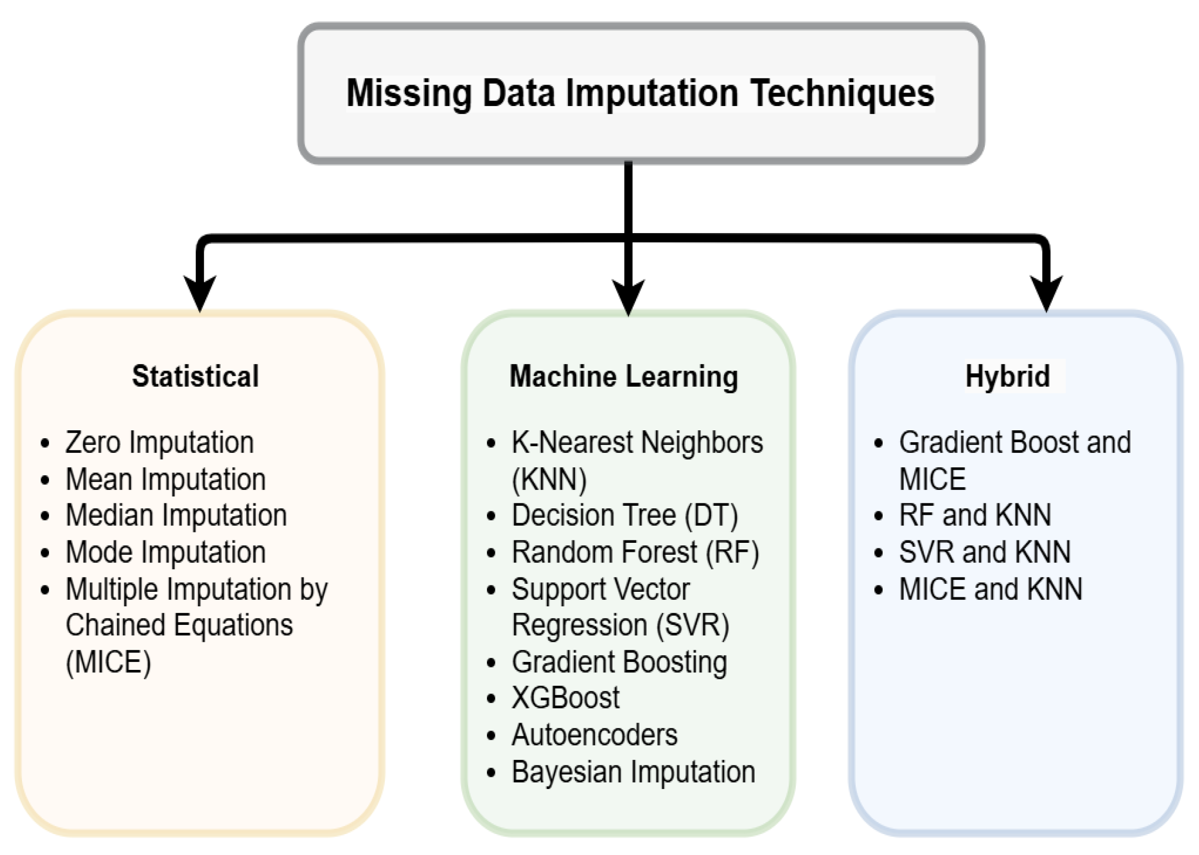
2.1. Statistical Techniques for Missing Data Imputation

Statistical imputation methodologies provide basic and essential methods for estimating missing values based on fundamental characteristics of the data. In [15] proposes a novel seasonal based imputation model for missing electrical load data. Missing values are replaced using the mean, mean with standard deviation, and third quartile. Testing three different missing data placements and various proportions, results show that mean imputation is best for front and middle gaps, while the third quartile better at the end, outperforming complex methods. Analysis of the eight advanced statistical imputation techniques, including linear and bilinear ones, is used to preprocess the publicly accessible datasets of Belgian smart meters. The work findings suggest that the bilinear imputation technique outperforms the linear one when dealing with larger blocks of missing data, enabling an accuracy reconstruction of the smart meter data [16]. In [17], a new imputation method founded on Multivariate Adaptive Regression Splines (MARS) is presented and compared to the Multiple Imputation by Chained Equations (MICE) technique, showing that MARS provides the better accuracy in estimating missing values.

2.2. Machine Learning Techniques for Missing Data Imputation

Methods for managing missing data within ML-driven energy benchmarking models utilize a missing at random (MAR) perspective. A comparison of XGBoost’s built-in imputation with the Median, KNN, and classification and regression trees (CART) techniques reveals that CART most effectively maintains data distribution, thereby improving forecasting model performance. The results offer recommendations for choosing imputation techniques to enhance benchmarking precision [5]. Another ML-oriented imputation strategy for addressing missing data specifically employs KNN and SKNN algorithms. In contrast to the list-wise deletion (LD) approach, the findings indicate that SKNN performs better as compared to the both LD and the KNN in data imputation, boosting accuracy across various datasets and classification algorithms (SVM and decision tree) [18]. An array of regression-based ML algorithms are used for the estimation of missing data for imputation within IoT frameworks, including SVR, DTR, Ridge Regression, KNN, MissForest, and XGBoost. The findings demonstrate that Ridge Regression outperforms the other models significantly, achieving the most accurate RMSE and $R^2$ metrics for filling in missing sensor data in time-series datasets sourced from a real-time IoT environment [19]. In [20], researchers review statistical (ARIMA and LI) and ML (KNN, MLP, and SVR) imputation techniques for managing incomplete electric power data during seasonal and peak/off-peak intervals. The findings indicate that ML methods, especially KNN and SVR, are more effective than the statistical approaches, with KNN particularly exceptional during peak periods and LI proving more effective for off-peak and semi-peak times.

2.3. Deep Learning Techniques for Missing Data Imputation

The innovative DL models of SAITS and USGAN have been analyzed for the purpose of imputing multivariate time series data in electrical energy consumption. Utilizing electrical load data subjected to varying degrees of data loss (10–50%), the models show effective imputation, providing significant insights for enhancing energy management and sustainability in educational organizations [21]. In one approach [22], a back-propagation artificial neural network was employed to resolve categorical missing data, analyzing the model’s performance relative to multiple imputation and random forest approaches. The results demonstrate that the neural network consistently outperforms other methods, confirming its reliability as a technique for reconstructing missing values in multivariate analyses. Advanced DL-driven forecasting models aim at predicting electrical load, supporting cost efficiency and effective distribution. Among the assessed models (LSTM, GRU, and RNN), the GRU exhibited notably enhanced performance [23]. An LSTM-based forecasting model designed for the load of EV charging stations was introduced, and an imputation technique to manage missing data was integrated. The experimental findings reveal that the proposed imputation strategy markedly enhances forecasting accuracy, decreasing errors by as much as 9.8% in comparison to models lacking imputation [24]. Another study investigated and examined advanced DL algorithms aimed at the estimation of absent data within the context of low-energy data aggregation, a domain in which traditional methodologies exhibit limitations. A multi-layer perceptron in combination with deep neural networks allows for the forecasting and correction of missing data, thus increasing accuracy when compared to conventional strategies. The results demonstrate that DL has the potential to improve energy efficiency and data reliability in low-energy scenarios [25].

2.4. Hybrid Model Techniques for Missing Data Imputation

Hybrid ML frameworks are designed to impute missing power load data by merging the random forest (RF), Soft Weight K-Nearest Neighbors (SW-KNN), and Levenberg–Marquardt Backpropagation (LM-BP) methods using a variance–covariance weighted approach for the dynamic adjustment of parameters. The findings presented in [26] indicate that the inclusion of meteorological and temporal variables leads to a reduction in errors ranging from 8% to 38%, while the hybrid model enhances predictive accuracy by 12% to 24% compared to single-model strategies. In [27], a sophisticated electricity price prediction model was developed that includes bidding behaviors and market sentiment. It utilizes the enhanced predictive features of a refined Large Language Model (LLM), which contributes to forecasting bidding behaviors and performing sentiment analysis to improve overall predictability. Moreover, the enhanced Conditional Time Series Generative Adversarial Network (CTSGAN) model is better at predicting price spikes, providing a robust tool for practitioners of the high-frequency Australian National Electricity Market (NEM). The proposed methodology involves the configuration of Bidirectional Long Short-Term Memory (BiLSTM) and a Bidirectional Gated Recurrent Unit (BiGRU), trained on a fully connected layer using clean datasets. The forecasting model presented in [28] utilizes the temporal relationships inherent in the data to deliver highly accurate predictions. In this context, a DL model that integrates autoencoders and LSTM is employed for forecasting missing load data. The combination of the Denoising Convolutional Autoencoder (DCAE) with LSTM significantly enhances forecasting precision as discussed in [29]. A comparative assessment of DL architectures is proposed in [30], where artificial neural network (ANN)–multi-layer perceptron (MLP), recurrent neural network (RNN)–LSTM, and one-dimensional convolutional neural network (1D-CNN) models were analyzed in order to perform both short- and medium-term electrical load forecasting. Based on the evaluation metrics, the results demonstrate that the 1D-CNN utilizing the MTAP methodology achieves superior accuracy. Reference [31] relates to hybrid forecasting for renewable and non-renewable energy data through a hybrid approach that helps in the case of challenges caused by variability in electric grids. This work proposes the EEMD-SVR model, which combines ensemble empirical mode decomposition (EEMD) and SVR, as well as the BiLSTM-AM model, which incorporates bidirectional LSTM with an attention mechanism (BiLSTM-AM). Experimental results using wind speed datasets demonstrate a significant reduction in error and prove the efficiency of the model in capturing energy patterns that can be useful for the advancement of smart grids.

2.5. Why LSTM Is the Preferred Model for MTLF

The preference of long short-term memory (LSTM) networks over other deep learning models like Gated Recurrent Units (GRUs) and Transformer models in particular applications can be attributed to specific advantages that LSTM networks provide in the analysis of the time series data. Although each model has its strengths, LSTM networks are often preferred due to their ability to capture long-term dependencies and their robustness in various contexts, particularly in financial and time series forecasting tasks [32,33]. This flexibility enables LSTM networks to be integrated into more advanced architecture (e.g., CNN-LSTM-GRU networks) that leverage their strengths alongside other models [34]. This preference is influenced by the specific requirements of the task, such as the need for capturing temporal dependencies, model complexity, and computational efficiency.

2.6. Forecasting Model: Long Short-Term Memory (LSTM)

For energy consumption forecasting, a special kind of recurrent neural network, namely, an LSTM, is selected. This study is based on LSTM networks, types of temporal cyclic neural networks specifically developed to solve the long-term dependence problem, that is, a general RNN (recurrent neural network). A memory unit replaces the hidden layer neurons of a regular RNN network in an LSTM network. Memory unit architecture, such as the input gate, forgetting gate, and output gate, enables the networks to discard irrelevant data and preserve important data at every time step. This is due to the ability to learn temporal correlations, and such timing correlates are relevant in power consumption loads as they rely on inhabitants’ behavior that is difficult to understand and predict. For example, in the electrical load forecasting problem, the role of the LSTM network is to identify the phases of the loads from behaviors of the incoming power consumption profile, capturing this state in memory, and then predicting based on the knowledge gained [35].

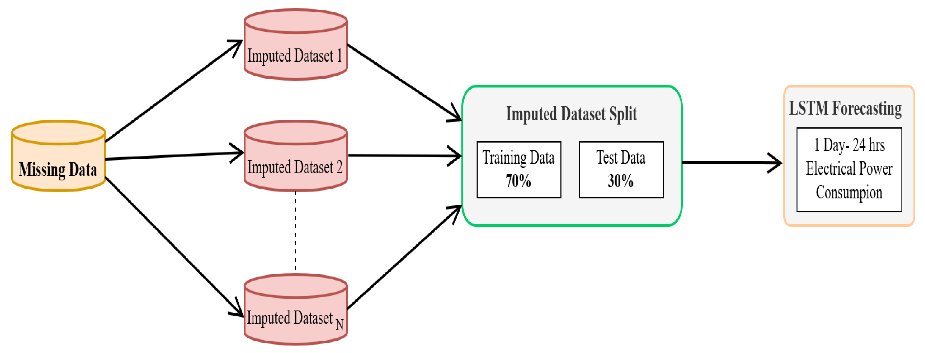
3. Selected Methodology

In the data extraction stage, an initial dataset with no missing values is used prior to the collection and data cleaning process. The electrical power consumption data are aggregated from the smart circuit breakers, communication devices, and cloud databases from the smart commercial building in Bergamo (Italy). The hourly electrical load data cover the period from the 1 January till 31 December 2023. The overall initial dataset (without missing data) contains 8760 rows and 11 columns, and an example of such a data structure is given in

Table 1. Example of data records (linear parameters).

Date	Time	${\mathbf{P}}_{\mathbf{Avg}}$ (kW)	${\mathbf{P}}_{\mathbf{Min}}$ (kW)	${\mathbf{P}}_{\mathbf{Max}}$ (kW)	${\mathbf{Q}}_{\mathbf{Avg}}$ (kvar)	${\mathbf{Q}}_{\mathbf{Min}}$ (kvar)	${\mathbf{Q}}_{\mathbf{Max}}$ (kvar)	${\mathbf{S}}_{\mathbf{Avg}}$ (kVA)	${\mathbf{S}}_{\mathbf{Min}}$ (kVA)	${\mathbf{S}}_{\mathbf{Max}}$ (kVA)
15 January 2023	09:00:00	137	101	212	9	3	19	140	104	216
15 January 2023	10:00:00	229	204	257	22	19	26	233	207	261
15 January 2023	11:00:00	197	170	229	18	14	21	201	174	233
15 January 2023	12:00:00	195	170	223	17	14	21	199	174	227
15 January 2023	13:00:00	187	165	205	17	14	19	190	168	209

[36].

Table 2. Weather data (nonlinear parameters).

Date	Time	Temp. (°C)	All Sky Irr. (W/m²)	Humid. (%)	Wind (m/s)	Clear Sky Irr. (W/m²)
15 January 2023	09:00:00	6.11	70.3	89.82	1.22	136.3
15 January 2023	10:00:00	7.11	97.68	83.64	1.74	249.75
15 January 2023	11:00:00	8.07	122.05	81.94	1.63	324.15
15 January 2023	12:00:00	8.65	154.43	79.97	1.28	362.77
15 January 2023	13:00:00	8.95	73.88	78.56	1.16	336.23

illustrates a dataset that includes five entries of nonlinear weather parameters, including temperature, humidity, wind speed, and irradiance for the year 2023. These data were obtained from the NASA POWER (Prediction of Worldwide Energy Resource), which offers high-quality global weather and climate data that can be used for many research purposes [37]. The weather data are particularly valuable for analyzing the impact of meteorological factors on smart commercial building energy consumption and the potential energy production from solar power. Table 1 and Table 2 are merged to give information (date, hour, day, month, year) for each record, which provides a better understanding of how changes occurred throughout the year with reference to the data.

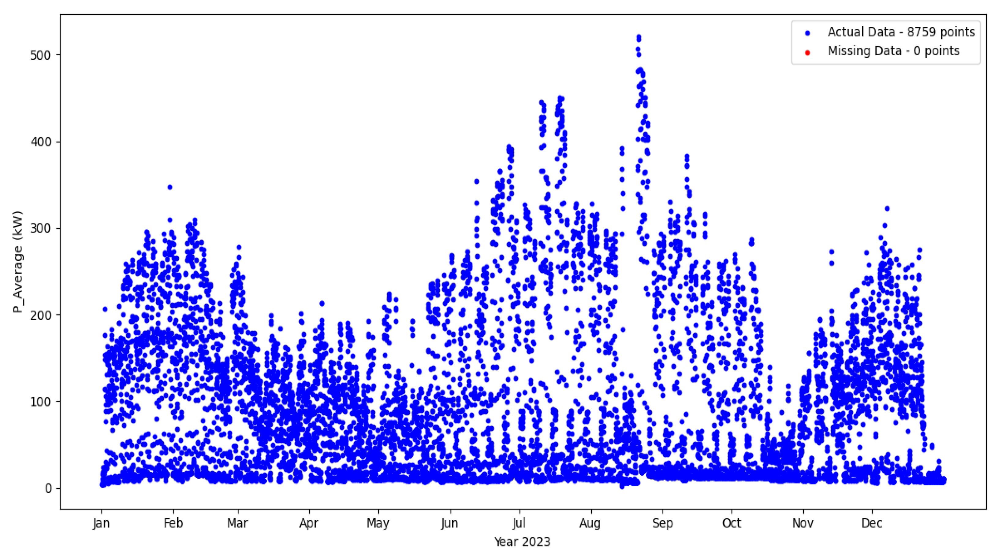
3.1. Data Preprocessing

Data preprocessing represents a fundamental step in the preparation of the dataset for subsequent and effective analytical tasks. Essential processes such as feature scaling, normalization, and the handling of missing values are incorporated to ensure that the data are suitably formatted and free from anomalies or inconsistencies. In this phase, preprocessing methodologies are implemented on the dataset to identify and eliminate outliers through the application of the inter-quartile range. In Figure 1, the target variable, namely, the active average power consumption in 2023, is shown without missing values or outliers.

3.2. Feature Engineering

Data feature engineering for exploratory data analysis ensures the successful prediction performance and interpretability of forecasting models by converting raw data to relevant features. It can enhance model accuracy, lower the complexity of computation, and prevent overfitting by carefully choosing and processing input variables [38]. Some effective feature engineering techniques include statistical transformations, lag time-based encoding, feature generation, and correlation analysis. All these techniques are used to generate more robust forecasting models. In this study, a correlation matrix was employed to assess the relationship among useful variables.

$$r={\displaystyle \frac{\sum (x_i-\overline{x})(y_i-\overline{y})}{\sqrt{\sum {(x_i-\overline{x})}^2\sum {(y_i-\overline{y})}^2}}}$$

(4)

In Equation (4), r is the correlation coefficient, $x_i$ represents the values of the x-variable in a sample, and $\overline{x}$ is the mean of the x-variable values. Similarly, $y_i$ refers the values of the y-variable in a sample, while $\overline{y}$ is the mean of the y-variable values. This equation is applied to check the correlation between two variables [39].

The heatmap plot in Figure 2 shows the correlation between the feature variables within the dataset. The features were selected based on a positive correlation range of 0.88 to 0.29, with variables outside this range excluded because of negative or weak correlation. Active power $P_{\mathrm{avg}}$ is considered as the target variable for electrical load forecasting. To ensure a balanced feature selection process, one reactive power component was chosen $Q_{\mathrm{avg}}$ as a linear feature, while the other linear parameters were neglected to reduce model redundancy and bias. The remaining selected features were drawn from nonlinear variables, including meteorological factors such as temperature at 2 m, humidity at 2 m, solar irradiance (both all-sky surface and clear-sky surface), and wind speed at 10 m. This approach aims to enhance the accuracy and generalization capability of the forecasting model while maintaining computational efficiency components.

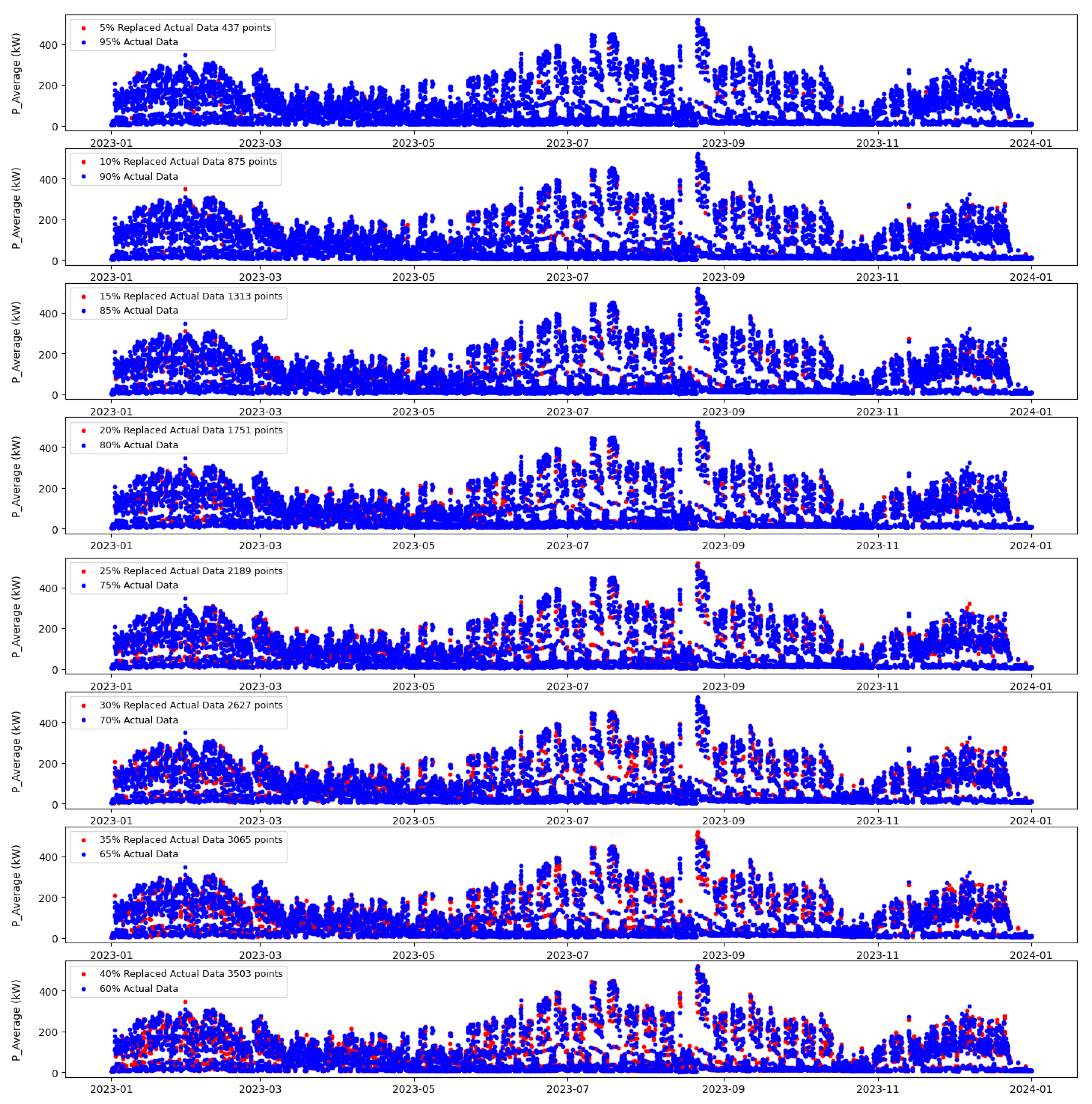
3.3. Assigning Random Missing Values

The original dataset in Figure 1, which contains no missing values or outliers, was initially used for MTLF purposes using an LSTM neural network. The resulting electric load prediction represents the reference for evaluating the forecasting performance in the case of missing values for different imputation methods. Starting from the initial dataset without missing values, as shown in Figure 1, randomly distributed missing data, which introduce biases, were intentionally integrated into the original dataset to emulate sensing equipment malfunctions and issues in the communication system. The individual missing data points were generated by replacing the original values with zero. To enhance the randomness, a methodology that involves multiple seeds or no seed was applied while adjusting the amount of missing data. The was achieved by repeating the procedure several times in order to artificially generate 8 datasets with the same size as the original dataset and featuring a variable ratio of missing data ranging from 5% to 40% with an incremental step of 5%, as shown in Figure 2. This approach will allow the systematic assessment of how the incomplete dataset affects the electric load forecast. Further, the availability of more datasets with different percentages of missing data would allow the critical level of missing data (i.e., max percentage of missing points before the load forecast significantly degrades) to be determined for the LSTM [40,41]. The 8 datasets in Figure 3 including the missing data were processed using imputation techniques and were finally used as input for the LSTM recurrent neural network.

3.4. Data Imputation Techniques

The datasets containing the missing data were created and preprocessed prior to being input into the forecasting model LSTM. Dataset preprocessing ensures consistency of the input data and proper handling of the missing values. For this purpose [42], various imputation techniques (i.e., statistical, ML, and hybrid) are considered in the presented comparative analysis in order to deliver a comprehensive investigation. Moreover, the effects of each method on the predictive performance are analyzed to determine their respective advantages and limitations. This step is critical for increasing the accuracy and robustness of forecasting models. In Figure 4, the selected imputation techniques (individual and integrated methods) are reported and classified according to their frameworks [43].

The statistical data imputation techniques used in this research include the following:

• Zero Imputation: Zero imputation is useful in some cases but also its has drawbacks. It assumes that missing values are similar to zero, which may not always hold true in every case and could result in biased forecasts. This imputation method can be applied but should be chosen based on the nature of the data and the needs of the particular forecasting task [44].
• Mean Imputation: One common method to deal with missing data is mean imputation, a method often used in electrical forecasting. This methodology [45] involves replacing missing values with the mean of the available data points. This is simply method but not necessarily the best approach for complex datasets such as electricity load forecasting datasets.
• Median Imputation: This technique is useful for handling missing data by replacing by the median of the available data. It is especially useful [46] for time-series data (for example, electricity load forecasting), where missing information can considerably impact the reliability of forecast results. Median imputation is also considered good and robust, especially for datasets containing outliers, since it is less affected by extreme values compared to mean imputation [47].
• Mode Imputation Mode imputation is a method of filling in missing values in a dataset by using the most common value. It is rather simple, and it is usually used in categorical data. On the other hand, its simplicity can bias the results if the data distribution is not uniform [48].
• Multiple Imputation: A probabilistic approach involving Multiple Imputation by Chained Equations (MICE), this methodology addresses [49] the issue of missing data through the generation of several complete datasets, analyzing each dataset independently and subsequently integrating the findings to mitigate the uncertainty associated in the missing data. This model is especially effective in situations where data integrity is vital for precise forecasting, like in energy management systems and electrical grid operations [50].

The AI/ML algorithms are used to perform missing value imputation that recognizes complex correlations present in datasets:

• K-Nearest Neighbor Imputation: The prediction methodology is a widely utilized similarity-based approach. In this context, the estimation of missing data can be achieved through the values of the K-nearest samples. This method computes the weighted mean of the neighboring samples, wherein the distance to these neighbors serves as the determining weights [51]. Consequently, the closer the neighbor, the greater the weight assigned in the aggregation process. Additionally [52], KNN is applicable in addressing both regression and classification challenges.
• Decision Tree: The decision tree approach creates a tree-like model in which each node in the tree corresponds to a decision to be made based on some features, and each leaf node corresponds to an outcome. This technique is highly applicable due to its capacity to work with nonlinear datasets and provide interpretable results. In dealing with noisy data or a very complex tree, this technique tends to overfit the data. However, this can be mitigated by using techniques such as integrating decision trees into ensemble models like random forest, which combine multiple trees to improve generalization and robustness [53].
• Random Forest: It constructs multiple decision trees, where each tree is trained on a random subset of the data, and makes predictions by combining the outputs of individual trees. This randomness helps in preventing overfitting and thus enhances model generalization. It is versatile since the algorithm can manage both numeric and categorical data. It is well known for its high accuracy and robustness especially in the presence of noise, outliers, and missing values [54].
• Support Vector Regression: SVR is widely known as a classification technique that can be used for both classification and regression problems. It only requires the identification of different, continuous, and categorical variables. SVMs construct a hyperplane in multidimensional space to distinguish different classes, thus generating an optimal hyperplane using an iterative process that is then applied for the purpose of minimizing the error [55]. An SVM produces a maximum marginal hyperplane that best splits the dataset to separate the classes. The accuracy of SVMs [55] is better than that of the other classifiers like logistic regression and decision trees. SVR is well known for its kernel method for dealing with nonlinear input spaces and is applicable to a variety of uses.
• XGBoost: Extreme Gradient Boosting is a supervised ML algorithm used for the tasks of classification and regression. It is an enhanced version of gradient boosting and adds a number of state-of-the-art techniques to improve performance while preventing overfitting [56]. This method offers features such as regularization to control the complexity of the model, thus avoiding overfitting and the ability to handle missing data efficiently [57]. XGBoost has been one of the most widely used algorithms in ML competitions and real-world applications, providing consistent high accuracy and efficiency.
• Autoencoder: This model is a type of a neural network which is used for unsupervised learning, mainly for dimensionality reduction and anomaly detection. This approach encodes input into a compressed representation before decoding that back to the input space. Usually, this model is used to determine missing data in a dataset. Through the reduction in reconstruction error, autoencoders can effectively recover the missing values based on the derived features, thus making them applicable for complex variables with interrelationships [58].
• Bayesian Imputation Bayesian Neural Networks (BNNs) effectively tackle model uncertainty by acquiring distributions over their weights rather than relying on static values. Bayesian imputation is a efficient method if there is uncertainty about the missing values and relationships are not well defined between values. Because this method [59] addresses uncertainty in both the data and the model assumptions, it can provide more robust estimates that are particularly valuable when dealing with complex datasets where simple imputations may not be adequate.

Hybrid imputation is a combination of multiple methods of imputation where different methods are used to understand the accuracy and stability of the missing data. This method takes advantage of the combination of different kind of imputation methods like statistical methods and ML models. Through the integration of these different methods, hybrid imputation significantly elevates predictive accuracy and mitigates biases that may be incurred by individual techniques. Recent studies in the field of electrical load forecasting have demonstrated the effectiveness of hybrid imputation in resolving issues related to missing sensor data, resulting in improved predictive performance and increased system reliability. The following combinations have been explored:

• Gradient Boosting and MICE.
• Random forest and KNN.
• Support Vector Regression (SVR) and KNN.
• MICE and KNN.

3.5. Experimental Setup

Figure 5 illustrates the performance of the imputed dataset with respect to different percentages of error and various imputation techniques. The dataset was split into 70% for training and 30% for testing to evaluate prediction performance. The LSTM model was applied to estimate the active power consumption of a smart commercial building for a timeframe of the next 24 h. The effectiveness of each imputation methodology was assessed in terms of evaluation performance metrics, thereby providing a detailed assessment of their effects on forecasting accuracy.

3.6. Optimizing Hyperparameters in LSTM Model Design

Hyperparameter optimization in the LSTM network is an important aspect in improving the effectiveness of electrical load forecasting. However, the model’s performance is highly dependent on the tuning of its hyperparameters [60]. The tuning process relates to the optimal selection of a set of hyperparameters for the learning algorithm.

The model implemented in this work utilizes a stacked LSTM architecture consisting of two stacked LSTM layers, where the first LSTM layer has 50 neurons and returns sequences serving as the needed sequence input for the second LSTM layer. The second LSTM layer also has 50 neurons and does not return sequences and a dropout layer with a 0.2 rate to avoid overfitting. The output is a dense layer with 25 neurons and a single neuron for predicting the target variable. The LSTM layers use their default hyperbolic tangent (tanh) activation function, which is typical for LSTM networks. Using the Adam optimizer with a learning rate of 0.0001 and mean squared error (MSE) as loss functions suitable for the regression task, we trained the model in batches of 32 for 20 epochs, and we evaluated its performance with a validation set. The decision regarding the number of epochs was based on an experimental investigation demonstrating that an increase in epochs failed to provide notable performance enhancement, thereby extending the training duration [61,62].

This architectural framework and configuration of hyperparameters were selected on the basis of empirical findings and computational efficiency, effectively performance metrics with training duration.

3.7. Evaluation Metrics

To assess the impact of missing data randomness on forecasting accuracy, the following key performance metrics were chosen for evaluating the LSTM recurrent neural network:

• Mean squared error (MSE) measures the average squared difference between predicted and actual values, providing insight into overall prediction accuracy as shown in Equation (5). This is the most common metric for measuring the amount of error in a model. MSE provides a measure of the average squared deviation of the model’s predictions from the observed data points [63].

  $$\mathrm{MSE}={\displaystyle \frac{1}{N}}\sum _{i=1}^N{(y_{\mathrm{test}}-y_{\mathrm{prediction}})}^2$$

  (5)
• Root mean squared error (RMSE) represents the square root of the average squared difference between predicted and actual values. It retains the same unit as the original data, making error interpretation more intuitive [64]. RMSE is a widely used metric in statistics and ML models for measuring the difference between predicted values and actual values. The formula for calculating RMSE is given in Equation (6).

  $$\mathrm{RMSE}=\sqrt{{\displaystyle \frac{1}{N}}\sum _{i=1}^N{(y_{\mathrm{test}}-y_{\mathrm{prediction}})}^2}$$

  (6)
• Mean Absolute Percentage Error (MAPE) evaluates the relative error percentage, making it useful for understanding the scale of forecasting deviations. MAPE is another commonly used metric in load forecasting. It measures the percentage difference between the predicted and actual values, providing a relative measure of accuracy as formulated in Equation (7). The MAPE metric is utilized to assess the relative accuracy of the ML models in load prediction [65].

  $$\mathrm{MAPE}={\displaystyle \frac{1}{N}}\sum _{i=1}^N\left({\displaystyle \frac{y_{\mathrm{test}}-y_{\mathrm{prediction}}}{y_{\mathrm{test}}}}\right)\times 100$$

  (7)

  with N the size of data, $y_{\mathrm{test}}$ the actual test value, and $y_{\mathrm{prediction}}$ the forecasting or prediction value.

4. Comparative Analysis Results and Discussion

Once the key performance parameters had been selected (i.e., MSE, RMSE, and MSE), the comparative investigation among different data imputation methods (i.e., statistical, ML, and hybrid methods) was carried out, and the electric load prediction and computational time were estimated using the LSTM MTLF model. The obtained outcomes are summarized in tables as well as figures, each representing a different data imputation technique.

In order to demonstrate the estimated accuracy and effectiveness of various imputation techniques,

Table 3. LSTM MTLF Forecasting Without Missing Data.

Metric Parameter	No Missing Data
MSE	884.977
RMSE	29.93
MAPE (%)	41.145

illustrates the performance evaluation metrics on the basis of the LSTM model for the forecasting of the next 24 h of electrical load. Furthermore, the table incorporates the performance metrics without missing data as a standard for comparative analysis.

In

Table 4. Statistical imputation techniques for LSTM forecasting.

Method	Time Avg. (s)	Metric Parameter	Missing Data Percentage
			5%	10%	15%	20%	25%	30%	35%	40%
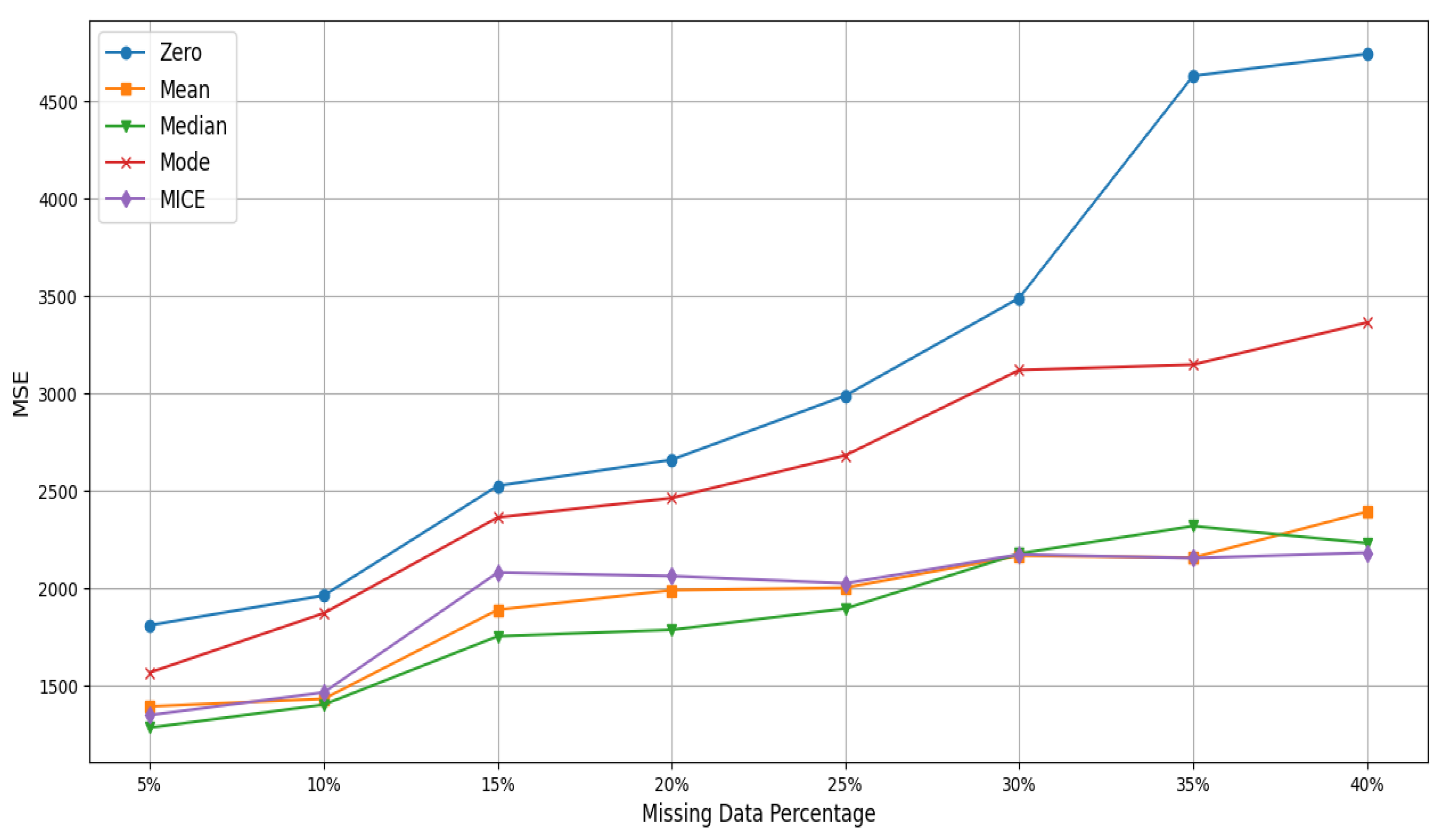
Zero	110.148	MSE	1811.47	1964.297	2527.194	2660.593	2990.181	3491.397	4631.182	4744.172
		RMSE	42.561	44.32	50.271	51.581	54.683	59.088	68.053	73.878
		MAPE (%)	$4.71\times {10}^8$	$6.89\times {10}^8$	$9.74\times {10}^8$	$1.09\times {10}^9$	$1.58\times {10}^9$	$2.01\times {10}^9$	$2.74\times {10}^9$	$3.12\times {10}^9$
Mean	115.843	MSE	1394.641	1433.627	1890.658	1991.166	2004.004	2168.529	2158.41	2394.124
		RMSE	37.345	37.863	43.482	44.622	44.766	46.567	46.459	48.93
		MAPE (%)	66.4	100.079	81.509	107.657	130.342	147.108	138.992	165.75
Mode	140.872	MSE	1569.351	1873.432	2364.658	2464.259	2683.373	3121.101	3148.997	3365.561
		RMSE	39.615	43.283	48.628	49.641	51.801	55.867	56.116	58.013
		MAPE (%)	88.913	129.123	125.92	188.14	188.304	197.165	173.295	246.58
Median	147.016	MSE	1285.373	1403.908	1754.768	1787.886	1897.027	2179.377	2320.485	2232.656
		RMSE	35.852	37.469	41.89	42.283	43.555	46.684	48.171	47.251
		MAPE (%)	64.944	70.161	77.546	91.736	82.422	98.113	83.282	85.52
MICE	138.633	MSE	1350.284	1466.694	2082.051	2063.719	2026.765	2174.838	2156.248	2183.75
		RMSE	36.746	38.297	45.629	45.428	45.02	46.635	46.435	46.731
		MAPE (%)	88.923	79.884	170.037	100.318	95.495	134.828	139.761	139.34

and Figure 6, the results of the statistical imputation methods are listed. The findings for the statistical imputation methods for handling missing data reveal that the forecasting errors increase as the percentage of missing data rises. This pattern is reflected in the increasing values of evaluation parameters and the average execution time required. However, the extent of performance degradation varies among different imputation techniques. Simple statistical data imputation methods such as zero and mode imputation methods experience significant error increases with the increase in the quantity of missing data and particularly zero imputation in terms of MAPE having the worst response and being unstable in any case of missing data. In terms of computational time, whereas mode and median imputation require more processing time, they have better results in terms of missing data. MICE offers a balance between accuracy and efficiency, making it a suitable statistical imputation method for handling missing data.

Table 5. ML imputation techniques for LSTM forecasting.

Method	Time Avg. (s)	Metric Parameter	Missing Data Percentage
			5%	10%	15%	20%	25%	30%	35%	40%
SVR	130.161	MSE	903.844	1043.156	1024.665	1105.509	1129.354	1083.008	1049.756	1139.506
		RMSE	30.064	32.298	32.01	33.249	33.606	32.909	32.4	33.757
		MAPE (%)	75.231	65.455	109.563	67.108	113.264	71.852	69.967	110.717
DT	133.506	MSE	972.27	1187.604	1253.919	1219.31	1312.045	1379.52	1243.631	1546.253
		RMSE	31.181	34.462	35.411	34.919	36.222	37.142	35.265	39.322
		MAPE (%)	68.566	65.363	81.329	49.399	82.121	66.419	82.967	112.748
RF	134.410	MSE	931.825	1122.079	1032.019	1096.043	1053.758	1096.904	1081.073	1150.148
		RMSE	30.526	33.497	32.125	33.107	32.462	33.12	32.88	33.914
		MAPE (%)	46.221	85.12	55.141	81.409	71.61	70.817	86.742	81.058
kNN	185.245	MSE	924.117	1042.867	1058.853	1185.159	1227.086	1220.965	1059.614	1210.18
		RMSE	30.399	32.293	32.54	34.426	35.03	34.942	32.552	34.788
		MAPE (%)	60.965	64.197	58.366	92.701	100.489	101.623	44.841	48.697
XGBoost	131.341	MSE	972.851	1051.04	1099.579	1092.893	1122.374	1113.451	1152.888	1211.747
		RMSE	31.191	32.42	33.16	33.059	33.502	33.368	33.954	34.81
		MAPE (%)	84.326	38.351	90.332	68.458	89.818	59.932	74.115	91.717
Autoencoder	108.782	MSE	1043.464	1041.291	1087.503	1070.714	1048.222	1142.464	1022.913	1168.709
		RMSE	32.303	32.269	32.977	32.722	32.376	33.8	31.983	34.186
		MAPE (%)	80.363	66.958	48.543	56.856	74.703	84.887	48.942	90.364
Gradient Boost	140.399	MSE	939.607	1026.154	1023.307	1077.813	1065.24	1011.671	1037.875	1047.425
		RMSE	30.653	32.034	31.989	32.83	32.638	31.807	32.216	32.364
		MAPE (%)	79.739	61.302	56.225	74.629	78.847	60.596	81.131	66.924
Bayesian	210.217	MSE	980.872	1063.451	1196.004	1248.85	1415.374	1217.751	1352.565	1358.912
		RMSE	31.319	32.611	34.583	35.339	37.621	34.896	36.777	36.863
		MAPE (%)	61.901	72.142	86.168	72.114	98.834	64.922	57.664	64.607

and Figure 7 summarize the outcomes obtained through ML-based imputation techniques. At first sight, the ML-based imputation techniques appear to deliver more accurate electric load predictions at higher missing data percentages and lower computational time. Among them, the SVR, random forest, and autoencoder approaches demonstrate the most consistent, accurate performance and low computational time, while Gradient Boosting maintains lower metric parameters and slightly high execution time across missing data proportions.

On the other hand, XGBoost performs well at lower to moderate missing data levels but experiences a sharp increase in errors beyond 30% missing data, making it less reliable in highly incomplete datasets. Meanwhile, K-NN and Bayesian imputation show their ineffectiveness in handling high proportions of missing values, resulting in poor accuracy. These models struggle significantly with an increase in missing data, showing much higher error values across the metrics.

The ML imputation results show that Gradient Boosting had a stable performance across various evaluation metrics, indicating that it is a robust model for forecasting tasks with missing datasets. Additionally, its ability to perform well at both high and low missing data percentages without major performance degradation makes it a reliable model for real-world applications where missing data are inevitable.

Finally, the performance associated with the hybrid data imputation techniques is reported in

Table 6. Hybrid imputation techniques for LSTM forecasting.

Method	Time Avg. (s)	Metric Parameter	Missing Data Percentage
			5%	10%	15%	20%	25%	30%	35%	40%
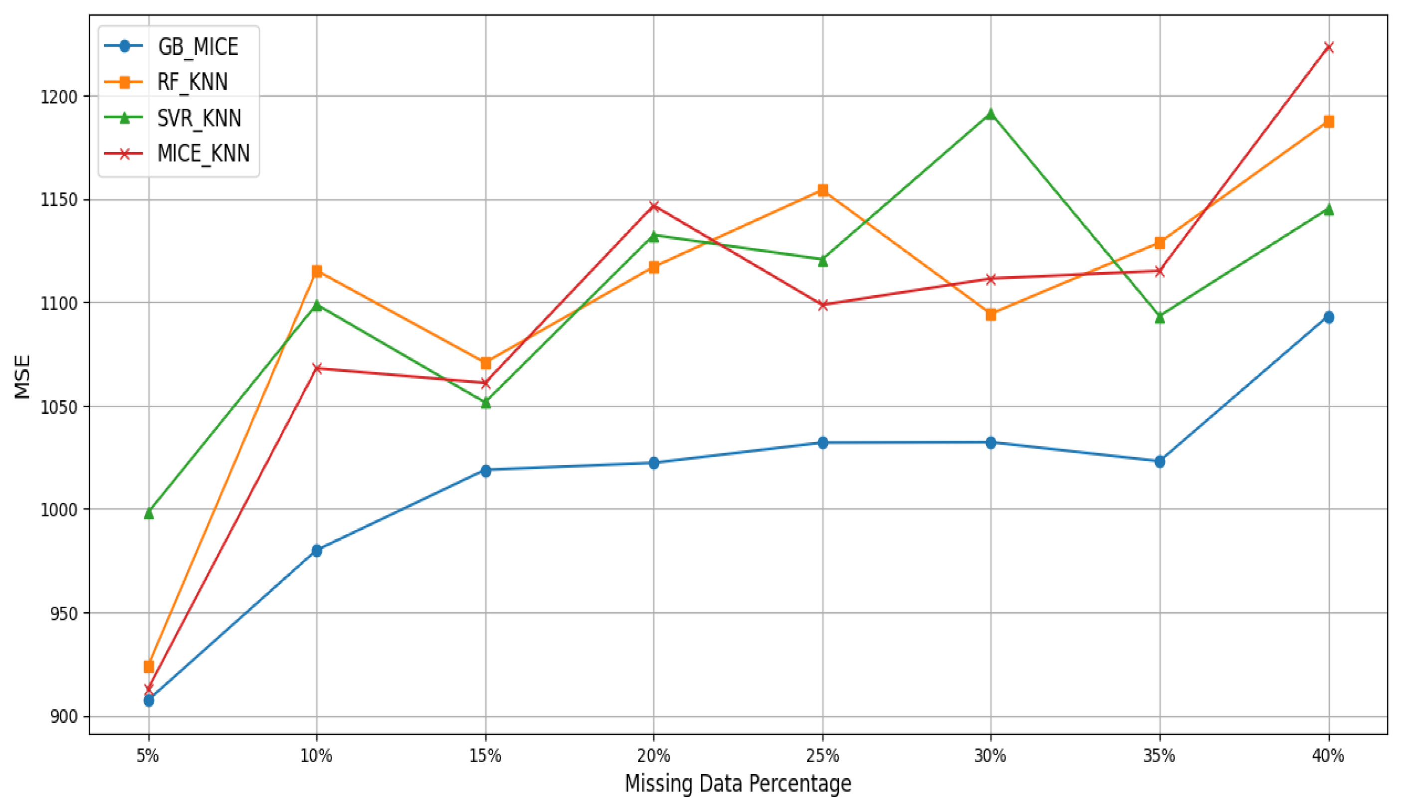
GB and MICE	90.472	MSE	907.344	979.976	1018.83	1022.219	1032.026	1032.224	1023.011	1093.231
		RMSE	30.122	31.305	31.919	34.96	32.125	32.128	31.985	33.064
		MAPE (%)	63.191	54.777	58.814	89.471	64.361	58.845	72.072	83.6
RF and KNN	125.420	MSE	923.789	1115.258	1070.743	1116.988	1154.157	1094.315	1128.762	1187.418
		RMSE	30.394	33.395	32.722	33.421	33.973	33.08	32.074	34.459
		MAPE (%)	78.699	83.333	68.362	70.613	92.917	60.912	51.908	85.965
SVR and KNN	129.509	MSE	998.064	1098.811	1051.478	1132.401	1120.637	1191.336	1093.245	1145.111
		RMSE	31.592	33.148	32.427	33.651	33.476	35.935	33.064	33.839
		MAPE (%)	69.468	43.326	40.826	48.223	80.226	103.752	84.974	61.438
MICE and KNN	124.467	MSE	912.786	1067.978	1060.892	1146.699	1098.613	1111.362	1115.061	1223.348
		RMSE	30.212	32.68	32.571	33.863	33.145	33.337	33.393	34.976
		MAPE (%)	49.876	52.032	57.212	79.368	64.084	63.138	58.423	94.029

and Figure 8. The results indicate that the combination of Gradient Boosting (GB) and MICE stands out for its consistent performance across different levels of missing data, with moderate increases in error metrics (MSE, RMSE, and MAPE) as the missing data percentage rises. This method strikes a good balance between computational efficiency, taking an average of 90.472 s, and accuracy. In contrast, the random forest (RF) and KNN as well as SVR and KNN approaches show higher variability in performance, especially as missing data increase. Their error metrics rise more sharply, and MAPE fluctuates significantly, reflecting challenges with higher missing data proportions. MICE and KNN achieve good performance when the missing data level is lower and exhibits a significant drop in prediction accuracy for higher missing data percentages. The computational time for these methods is relatively high, with SVR and KNN requiring the most time. Overall, GB and MICE emerges as the most robust method, providing reliable predictions while being computationally efficient.

5. Conclusions and Future Work

The results of this study highlight that the selection of an appropriate data imputation method according to the percentage of missing data plays an important role in MTLF. Basic statistical methods are shown to be ineffective when dealing with a relatively high percentage beyond 30% missing data, and ML-based techniques prove to be more suitable options in such circumstances. In absolute terms, ML-based data imputation methods, such as the SVR, random forest, and autoencoder approaches, provide more accurate predictions and faster computation, with Gradient Boosting (GB) emerging as the most reliable model, maintaining stable performance across different missing data levels. Considering the hybrid data imputation strategies, those using the Gradient Boosting with MICE are proven to be the most accurate, reliable and computationally efficient over the entire range of missing data percentages investigated (5–40%). Therefore, ML-based and hybrid data imputation techniques combined in an LSTM prediction model appear to be the most suitable choice for robust MTLF in the case of datasets affected by missing data.

Future research should advance and expand ML and hybrid imputation techniques for diverse applications, optimizing them for other robust forecasting models like Transformers and GNNs. Emphasis should be placed on real-world testing applications such as energy community datasets to assess performance under complex missing data conditions. Developing a unified framework for selecting the best imputation method based on data characteristics will enhance robustness and adaptability. Advancing these areas will lead to more reliable imputation methods, improving predictive modeling and decision-making across industries.

References

- Xu, H.; Fan, G.; Kuang, G.; Song, Y. Construction and Application of Short-Term and Mid-Term Power System Load Forecasting Model Based on Hybrid Deep Learning. IEEE Access 2023, 11, 37494–37507. [Google Scholar] [CrossRef]
- Pazhoohesh, M.; Allahham, A.; Das, R.; Walker, S. Investigating the Impact of Missing Data Imputation Techniques on Battery Energy Management System. IET Smart Grid 2021, 4, 162–175. [Google Scholar] [CrossRef]
- Osman, M.S.; Abu-Mahfouz, A.M.; Page, P.R. A Survey on Data Imputation Techniques: Water Distribution System as a Use Case. IEEE Access 2018, 6, 63279–63291. [Google Scholar] [CrossRef]
- David, S.; Azariya, S.; Mohanraj, V.; Emilyn, J.J.; Jothi, G. A Comparison of Missing Data Handling Techniques. ICTACT J. Soft Comput. 2021, 11, 2433–2437. [Google Scholar]
- Farewell, D.; Daniel, R.; Seaman, S. Missing at Random: A Stochastic Process Perspective. arXiv 2018, arXiv:1801.06739. [Google Scholar]
- Carreras, G.; Miccinesi, G.; Wilcock, A.; Preston, N.; Nieboer, D.; Deliens, L.; Groenvold, M.; Lunder, U.; van der Heide, A.; Baccini, M.; et al. Missing Not at Random in End of Life Care Studies: Multiple Imputation and Sensitivity Analysis on Data from the ACTION Study. BMC Med Res. Methodol. 2021, 21, 13. [Google Scholar] [CrossRef]
- Lee, K.; Lim, H.; Hwang, J.; Lee, D. Evaluating Missing Data Handling Methods for Developing Building Energy Benchmarking Models. Energy 2024, 308, 132979. [Google Scholar] [CrossRef]
- Gautam, R.; Latifi, S. Comparison of Simple Missing Data Imputation Techniques for Numerical and Categorical Datasets. J. Res. Eng. Appl. Sci. 2023, 8, 468–475. [Google Scholar]
- Bahadure, N.B.; Khomane, R.; Raut, D.; Chendake, Y.; Routray, S.; Mishra, D.P. Regression Model Selection for Life Expectancy Prediction: A Comparative Analysis of Imputation Techniques. In Proceedings of the 2024 4th International Conference on Advanced Research in Computing (ICARC), Belihuloya, Sri Lanka, 21–24 February 2024; pp. 49–54. [Google Scholar] [CrossRef]
- Singh, M.; Maini, R. Missing Data Analysis for Electric Load Prediction with Whole Record Missing. Adv. Math. Sci. J. 2020, 9, 4015–4023. [Google Scholar]
- Ahn, H.; Sun, K.; Kim, K.P. Comparison of Missing Data Imputation Methods in Time Series Forecasting. Comput. Mater. Contin. 2022, 70, 767–779. [Google Scholar] [CrossRef]
- Nguyen, V.H.; Bui, V.; Kim, J.; Jang, Y.M. Power Demand Forecasting Using Long Short-Term Memory Neural Network based Smart Grid. In Proceedings of the 2020 International Conference on Artificial Intelligence in Information and Communication (ICAIIC), Fukuoka, Japan, 19–21 February 2020; pp. 388–391. [Google Scholar] [CrossRef]
- Thirunagalingam, A. Combining AI Paradigms for Effective Data Imputation: A Hybrid Approach. Int. J. Transform. Bus. Manag. 2024, 14, 49–58. [Google Scholar] [CrossRef]
- Kim, T.; Ko, W.; Kim, J. Analysis and impact evaluation of missing data imputation in day-ahead PV generation forecasting. Appl. Sci. 2019, 9, 204. [Google Scholar] [CrossRef]
- Kamisan, N.A.B.; Lee, M.H.; Hussin, A.G.; Zubairi, Y.Z. Imputation Techniques for Incomplete Load Data Based on Seasonality and Orientation of the Missing Values. Sains Malays. 2020, 49, 1165–1174. [Google Scholar] [CrossRef]
- Wu, J.; Koirala, A.; van Hertem, D. Review of Statistics-Based Coping Mechanisms for Smart Meter Missing Data in Distribution Systems. In Proceedings of the 2022 IEEE PES Innovative Smart Grid Technologies Conference Europe (ISGT-Europe), Novi Sad, Serbia, 10–12 October 2022. [Google Scholar] [CrossRef]
- Turrado, C.C.; Lasheras, F.S.; Calvo-Rollé, J.L.; Piñón-Pazos, A.J. A New Missing Data Imputation Algorithm Applied to Electrical Data Loggers. Sensors 2015, 15, 31069–31082. [Google Scholar] [CrossRef]
- Rizvi, S.T.H.; Latif, M.Y.; Amin, M.S.; Telmoudi, A.J.; Shah, N.A. Analysis of Machine Learning Based Imputation of Missing Data. Cybern. Syst. 2023, 1, 1–15. [Google Scholar] [CrossRef]
- Kalay, S.; Çinar, E.; Sarıçiçek, İ. A Comparison of Data Imputation Methods Utilizing Machine Learning for a New IoT System Platform. In Proceedings of the 2022 8th International Conference on Control, Decision and Information Technologies (CoDIT), Istanbul, Turkey, 17–20 May 2022; pp. 69–74. [Google Scholar] [CrossRef]
- Wang, M.C.; Tsai, C.F.; Lin, W.C. Towards Missing Electric Power Data Imputation for Energy Management Systems. Expert Syst. Appl. 2021, 174, 114743. [Google Scholar] [CrossRef]
- Diaz-Bedoya, D.; Philippon, A.; Gonzalez-Rodriguez, M.; Clairand, J.M. Innovative Deep Learning Techniques for Energy Data Imputation Using SAITS and USGAN: A Case Study in University Buildings. IEEE Access 2024, 12, 168468–168476. [Google Scholar] [CrossRef]
- Chhabra, G. Handling Missing Data through Artificial Neural Network. Commun. Appl. Nonlinear Anal. 2024, 31, 677–684. [Google Scholar] [CrossRef]
- Abumohsen, M.; Owda, A.Y.; Owda, M. Electrical Load Forecasting Using LSTM, GRU, and RNN Algorithms. Energies 2023, 16, 52283. [Google Scholar] [CrossRef]
- Lee, B.; Lee, H.; Ahn, H. Improving Load Forecasting of Electric Vehicle Charging Stations through Missing Data Imputation. Energies 2020, 13, 4893. [Google Scholar] [CrossRef]
- Thakur, G. Estimating Missing Data in Low Energy Data Aggregation Using Deep Learning Algorithms. In Proceedings of the 2024 3rd International Conference for Innovation in Technology (INOCON), Bangalore, India, 1–3 March 2024; pp. 1–6. [Google Scholar] [CrossRef]
- Hou, Z.; Liu, J. Enhancing Smart Grid Sustainability: Using Advanced Hybrid Machine Learning Techniques While Considering Multiple Influencing Factors for Imputing Missing Electric Load Data. Sustainability 2024, 16, 8092. [Google Scholar] [CrossRef]
- Lu, X.; Qiu, J.; Yang, Y.; Zhang, C.; Lin, J.; An, S. Large Language Model-Based Bidding Behavior Agent and Market Sentiment Agent-Assisted Electricity Price Prediction. IEEE Trans. Energy Mark. Policy Regul. 2024, 1, 1–13. [Google Scholar] [CrossRef]
- Iqbal, M.S.; Adnan, M.; Mohamed, S.E.G.; Tariq, M. A Hybrid Deep Learning Framework for Short-Term Load Forecasting with Improved Data Cleansing and Preprocessing Techniques. Results Eng. 2024, 24, 103560. [Google Scholar] [CrossRef]
- Park, K.; Jeong, J.; Kim, D.; Kim, H. Missing-Insensitive Short-Term Load Forecasting Leveraging Autoencoder and LSTM. IEEE Access 2020, 8, 206039–206048. [Google Scholar] [CrossRef]
- Battula, H.; Panda, D.; Konda, K.R. A Comparative Study of Forecasting Problems on Electrical Load Timeseries Data Using Deep Learning Techniques. TechRxiv 2023. [Google Scholar] [CrossRef]
- Gomez, W.; Wang, F.-K.; Lo, S.-C. A Hybrid Approach Based Machine Learning Models in Electricity Markets. Energy 2024, 289, 129988. [Google Scholar] [CrossRef]
- Xiao, J.; Bi, S.; Deng, T. Comparative Analysis of LSTM, GRU, and Transformer Models for Stock Price Prediction. In Proceedings of the DEBAI ’24: Proceedings of the International Conference on Digital Economy, Blockchain and Artificial Intelligence, Guangzhou, China, 23–25 August 2024. [Google Scholar]
- Gökçe, M.M.; Duman, E. A Deep Learning-Based Demand Forecasting System for Planning Electricity Generation. Kahramanmaraş Sütçü İmam Üniversitesi Mühendislik Bilimleri Dergisi 2024, 27, 511–522. [Google Scholar] [CrossRef]
- Dong, Y.; Zhong, Z.; Zhang, Y.; Zhu, R.; Wen, H.; Han, R. Intelligent Prediction Method of Hot Spot Temperature in Transformer by Using CNN-LSTM &GRU Network. In Proceedings of the 2023 International Conference on Advanced Robotics and Mechatronics (ICARM), Sanya, China, 8–10 July 2023; pp. 7–12. [Google Scholar] [CrossRef]
- Mubashar, R.; Awan, M.J.; Ahsan, M.; Yasin, A.; Singh, V.P. Efficient Residential Load Forecasting Using Deep Learning Approach. Int. J. Comput. Appl. Technol. 2022, 68, 205–214. [Google Scholar] [CrossRef]
- Hussain, A.; Franchini, G.; Giangrande, P.; Mandelli, G.; Fenili, L. A Comparative Analysis of Machine Learning Models for Medium-Term Load Forecasting in Smart Commercial Buildings. In Proceedings of the 2024 IEEE 12th International Conference on Smart Energy Grid Engineering (SEGE), Oshawa, ON, Canada, 18–20 August 2024; pp. 228–232. [Google Scholar] [CrossRef]
- Amin, A.; Mourshed, M. Weather and Climate Data for Energy Applications. Renew. Sustain. Energy Rev. 2024, 192, 114247. [Google Scholar] [CrossRef]
- Wen, Q.; Liu, Y. Feature Engineering and Selection for Prosumer Electricity Consumption and Production Forecasting: A Comprehensive Framework. Appl. Energy 2025, 381, 125176. [Google Scholar] [CrossRef]
- Zhang, J.; Xu, Z.; Wei, Z. Absolute logarithmic calibration for correlation coefficient with multiplicative distortion. Commun. Stat. Simul. Comput. 2020, 52, 482–505. [Google Scholar] [CrossRef]
- Emmanuel, T.; Maupong, T.; Mpoeleng, D.; Semong, T.; Mphago, B.; Tabona, O. A Survey on Missing Data in Machine Learning. J. Big Data 2021, 8, 140. [Google Scholar] [CrossRef] [PubMed]
- Farhangfar, A.; Kurgan, L.; Dy, J. Impact of Imputation of Missing Values on Classification Error for Discrete Data. Pattern Recognit. 2008, 41, 3692–3705. [Google Scholar] [CrossRef]
- Peppanen, J.; Zhang, X.; Grijalva, S.; Reno, M.J. Handling Bad or Missing Smart Meter Data through Advanced Data Imputation. In Proceedings of the 2016 IEEE Power & Energy Society Innovative Smart Grid Technologies Conference (ISGT), Minneapolis, MN, USA,, 6–9 September 2016; pp. 1–5. [Google Scholar] [CrossRef]
- Utama, A.B.P.; Wibawa, A.P.; Handayani, A.N.; Irianto, W.S.G.; Aripriharta; Nyoto, A. Improving Time-Series Forecasting Performance Using Imputation Techniques in Deep Learning. In Proceedings of the 2024 International Conference on Smart Computing, IoT and Machine Learning (SIML), Surakarta, Indonesia, 6–7 June 2024; pp. 232–238. [Google Scholar] [CrossRef]
- Khan, M.A. A Comparative Study on Imputation Techniques: Introducing a Transformer Model for Robust and Efficient Handling of Missing EEG Amplitude Data. Bioengineering 2024, 11, 740. [Google Scholar] [CrossRef]
- Twumasi-Ankrah, S.; Odoi, B.; Pels, W.A.; Gyamfi, E.H. Efficiency of Imputation Techniques in Univariate Time Series. Int. J. Sci. Environ. Technol. 2019, 8, 430–453. [Google Scholar]
- Schreiber, J.F.; Sausen, A.; Campos, M.D.; Sausen, P.S.; Da Silva Ferreira Filho, M.T. Data Imputation Techniques Applied to the Smart Grids Environment. IEEE Access 2023, 11, 31931–31940. [Google Scholar] [CrossRef]
- Pan, Z.; Wang, Y.; Wang, K.; Chen, H.; Yang, C.; Gui, W. Imputation of Missing Values in Time Series Using an Adaptive-Learned Median-Filled Deep Autoencoder. IEEE Trans. Cybern. 2023, 53, 695–706. [Google Scholar] [CrossRef]
- Memon, S.M.Z.; Wamala, R.; Kabano, I.H. A Comparison of Imputation Methods for Categorical Data. Informatics Med. Unlocked 2023, 42, 101382. [Google Scholar] [CrossRef]
- Phan, Q.-T.; Wu, Y.-K.; Phan, Q.-D.; Lo, H.-Y. A Study on Missing Data Imputation Methods for Improving Hourly Solar Dataset. In Proceedings of the Proceedings of the 2022 8th International Conference on Applied System Innovation (ICASI), Nantou, Taiwan, 22–23 April 2022. [CrossRef]
- Ruggles, T.; Farnham, D.J.; Tong, D.; Caldeira, K. Developing Reliable Hourly Electricity Demand Data Through Screening and Imputation. Sci. Data 2020, 7, 155. [Google Scholar] [CrossRef]
- Maillo, J.; Ramírez, S.; Triguero, I.; Herrera, F. kNN-IS: An Iterative Spark-based Design of the k-Nearest Neighbors Classifier for Big Data. Knowl.-Based Syst. 2017, 117, 3–15. [Google Scholar] [CrossRef]
- Halder, R.K.; Uddin, M.N.; Uddin, M.A.; Aryal, S.; Khraisat, A. Enhancing K-Nearest Neighbor Algorithm: A Comprehensive Review and Performance Analysis of Modifications. J. Big Data 2024, 11, 113. [Google Scholar] [CrossRef]
- Yaprakdal, F.; Bal, F. Comparison of Robust Machine-learning and Deep-learning Models for Midterm Electrical Load Forecasting. Eur. J. Tech. (EJT) 2022, 12, 102–107. [Google Scholar] [CrossRef]
- Wang, P.; Xu, K.; Ding, Z.; Du, Y.; Liu, W.; Sun, B.; Zhu, Z.; Tang, H. An Online Electricity Market Price Forecasting Method Via Random Forest. IEEE Trans. Ind. Appl. 2022, 58, 7013–7021. [Google Scholar] [CrossRef]
- Olawuyi, A.; Ajewole, T.; Oladepo, O.; Awofolaju, T.T.; Agboola, M.; Hasan, K. Development of an Optimized Support Vector Regression Model Using Hyper-Parameters Optimization for Electrical Load Prediction. UNIOSUN J. Eng. Environ. Sci. 2024, 6. [Google Scholar] [CrossRef]
- Liao, N.; Hu, Z.; Magami, D. A Metaheuristic Approach to Model the Effect of Temperature on Urban Electricity Need Utilizing XGBoost and Modified Boxing Match Algorithm. AIP Adv. 2024, 14, 115318. [Google Scholar] [CrossRef]
- Choi, D.K. Data-Driven Materials Modeling with XGBoost Algorithm and Statistical Inference Analysis for Prediction of Fatigue Strength of Steels. Int. J. Precis. Eng. Manuf. 2019, 20, 129–138. [Google Scholar] [CrossRef]
- Pajić, Z.; Janković, Z.; Selakov, A. Autoencoder-Driven Training Data Selection Based on Hidden Features for Improved Accuracy of ANN Short-Term Load Forecasting in ADMS. Energies 2024, 17, 5183. [Google Scholar] [CrossRef]
- Xu, L.; Hu, M.; Fan, C. Probabilistic Electrical Load Forecasting for Buildings Using Bayesian Deep Neural Networks. J. Build. Eng. 2022, 46, 103853. [Google Scholar] [CrossRef]
- Lu, N.; Ouyang, Q.; Li, Y.; Zou, C. Electrical Load Forecasting Model Using Hybrid LSTM Neural Networks with Online Correction. arXiv 2024, arXiv:2403.03898. [Google Scholar]
- Simani, K.N.; Genga, Y.O.; Yen, Y.-C.J. Using LSTM To Perform Load Predictions For Grid-Interactive Buildings. SAIEE Afr. Res. J. 2024, 115, 42–47. [Google Scholar] [CrossRef]
- Torres, J.F.; Martínez-Álvarez, F.; Troncoso, A. A Deep LSTM Network for the Spanish Electricity Consumption Forecasting. Neural Comput. Appl. 2022, 34, 10533–10545. [Google Scholar] [CrossRef] [PubMed]
- Shirzadi, N.; Nizami, A.; Khazen, M.; Nik-Bakht, M. Medium-Term Regional Electricity Load Forecasting through Machine Learning and Deep Learning. Designs 2021, 5, 27. [Google Scholar] [CrossRef]
- Almaghrebi, A.; Aljuheshi, F.; Rafaie, M.; James, K.; Alahmad, M. Data-Driven Charging Demand Prediction at Public Charging Stations Using Supervised Machine Learning Regression Methods. Energies 2020, 13, 4231. [Google Scholar] [CrossRef]
- Amber, K.P.; Ahmad, R.; Aslam, M.W.; Kousar, A.; Usman, M.; Khan, M.S. Intelligent Techniques for Forecasting Electricity Consumption of Buildings. Energy 2018, 157, 886–893. [Google Scholar] [CrossRef]