Event-Triggered Discrete-Time ZNN Algorithm for Distributed Optimization with Time-Varying Objective Functions

Abstract

This paper investigates discrete-time distributed optimization for multi-agent systems (MASs) with time-varying objective functions. A novel fully distributed event-triggered discrete-time zeroing neural network (ET-DTZNN) algorithm is proposed to address the discrete-time distributed time-varying optimization (DTDTVO) problem without relying on periodic communication. Each agent determines the optimal solutions by relying solely on local information, such as its own objective function. Moreover, information is exchanged with neighboring agents exclusively when event-triggered conditions are satisfied, significantly reducing communication consumption. The ET-DTZNN algorithm is derived by discretizing a proposed event-triggered continuous-time ZNN (ET-CTZNN) model via the Euler formula. The ET-CTZNN model addresses the time-varying optimization problem in a semi-centralized framework under continuous-time dynamics. Theoretical analyses rigorously establish the convergence of both the ET-CTZNN model and the ET-DTZNN algorithm. Simulation results highlight the algorithm’s effectiveness, precision, and superior communication efficiency compared with traditional periodic communication-based approaches.

1. Introduction

The rapid advancement of large-scale networks and the progress in big data theory have significantly fueled the exploration of distributed optimization algorithms. These algorithms have found widespread application across various scientific and engineering domains [1,2,3,4]. These algorithms prove particularly valuable in application contexts such as power economic dispatch [2], Nash equilibrium seeking [3], and smart grids [4]. Within distributed optimization architectures, the collective objective function of multi-agent networks emerges from the aggregated summation of individual agents’ local sub-objectives. During operational execution, each agent maintains exclusive access to its designated sub-objective function while implementing state information exchange protocols with neighbouring agents. The global optimal solution is attained through consensus across all participating agents [1]. Recent advancements in distributed optimization have focused on various innovative approaches to enhance efficiency and effectiveness. For example, Pan et al. presented a robust optimization method for active distribution networks with variable-speed pumped storage to mitigate the risks associated with new energy sources [5]. Another research by Luo et al. introduced a consensus-based distributed optimal dispatch algorithm for integrated energy microgrids, aiming to achieve economic operation and power supply–demand balance [6]. Additionally, Tariq et al. presented an optimal control strategy for centralized thermoelectric generation systems using the barnacles mating optimization algorithm to address nonuniform temperature distribution [7]. Further, Yang et al. proposed the heavy-ball Barzilai–Borwein algorithm, a discrete-time method combining the heavy-ball momentum and Barzilai–Borwein step sizes for static distributed optimization over time-varying directed graphs [8]. Lastly, a privacy-preserving distributed optimization algorithm for economic dispatch over time-varying directed networks was developed by An et al. to protect sensitive information while ensuring fully distributed and efficient operation [9].

While prior researches have extensively addressed distributed optimization with static objective functions, real-world implementations frequently necessitate handling distributed optimization problems where objective functions dynamically evolve through time [10,11,12,13]. While distributed static optimization problem deals with fixed objective functions, distributed time-varying optimization (DTVO) problem involves objective functions that change over time. This dynamic nature introduces several challenges, such as the need for continuous adaptation to changing conditions, ensuring convergence to time-dependent optimal solutions and maintaining communication efficiency among agents [12]. Recent advancements in the DTVO problem have introduced several innovative algorithms to address dynamic challenges. Zheng et al. proposed a specified-time convergent algorithm tailored for distributed optimization problems characterized by time-varying objective functions. This algorithm guarantees convergence within a predefined timeframe [14]. Wang et al. developed a distributed algorithm for time-varying quadratic optimal resource allocation, focusing on applications like multi-quadrotor hose transportation [15]. Ding et al. developed a distributed algorithm based on output regulation theory to handle both equality and inequality constraints in time-varying optimization problems [16]. Rahili et al. studied the time-varying distributed convex optimization problem for continuous-time multi-agent systems and introduced control algorithms for single-integrator and double-integrator dynamics [17].

Introduced by Zhang et al. in 2002 [18], zeroing neural network (ZNN) models and ZNN algorithms offer a solution for tackling a variety of challenging time-varying problems. Thanks to their ability to handle parallel computing, their suitability for hardware implementation, and their distributed nature, ZNN models have been extensively applied to solve various time-varying challenges since their creation [19,20,21,22]. Moreover, in recent years, researchers have introduced several innovative algorithms to address distributed time-varying problems. For example, Xiao et al. proposed a distributed fixed-time ZNN algorithm designed to achieve fixed-time and robust consensus in multi-agent systems under switching topology [22]. Liao et al. introduced a novel ZNN algorithm for real-time management of multi-vehicle cooperation, illustrating its effectiveness and robustness in achieving real-time cooperation among multiple vehicles [23]. Yu et al. presented a data-driven control algorithm based on discrete ZNN for continuum robots, ensuring real-time control and adaptability to varying conditions [24]. Jin et al. introduced a distributed approach to collaboratively generate motion within a network of redundant robotic manipulators, utilizing a noise-tolerant ZNN to handle communication interferences and computational errors [25].

The aforementioned distributed ZNN models and algorithms tackle continuous-time DTVO problems, and it is essential to develop discrete-time ZNN algorithms for the practical implementation of theoretical continuous-time solutions in digital systems, ensuring accurate and efficient real-time computations while leveraging the advantages of digital hardware [26]. While there are plenty researches on centralized discrete-time ZNN algorithms [26,27], research on distributed ZNN algorithms that tackles discrete-time distributed time-varying problems is scarce. Notably, conventional discrete-time ZNN algorithms predominantly employ periodic iteration mechanisms [26,27]. This architecture inherently incurs elevated communication consumption (if applied to distributed ZNN algorithms), particularly under small sampling intervals or reduced iteration step sizes, while communication consumption constitutes a critical performance metric for assessing distributed algorithmic efficacy. In contrast, event-triggered communication paradigms strategically regulate inter-agent data transmission through state-dependent triggering criteria, thereby achieving substantial communication efficiency gains. Therefore, some researchers have dedicated their efforts to event-triggered ZNN algorithms and the results have shown significant progress in addressing time-varying problems. For instance, Dai et al. introduced an adaptive fuzzy ZNN model integrated with an event-triggered mechanism to address the time-varying matrix inversion problem. Their approach achieved finite-time convergence and demonstrated robustness [28]. Kong et al. introduced a predefined time fuzzy ZNN algorithm with an event-triggered mechanism for kinematic planning of manipulators, ensuring predefined time convergence and reducing computational burden [29].

Motivated by the need to address the discrete-time DTVO (DTDTVO) problem, a novel event-triggered discrete-time ZNN (ET-DTZNN) algorithm is proposed. This algorithm is built upon an event-triggered continuous-time zeroing neural network (ET-CTZNN) model, which was specifically designed to address the continuous-time distributed time-varying optimization (CTDTVO) problem within a semi-centralized framework. By discretizing the ET-CTZNN model using the Euler formula, the ET-DTZNN algorithm enables agents to compute optimal solutions based on local time-varying objective functions and exchange information with neighbors only when specific event-triggered conditions are met. This algorithm significantly reduces communication consumption while preserving the temporal tracking capabilities inherent to ZNN algorithms. In this paper, the ET-DTZNN algorithm is designed to solve strongly convex distributed optimization problem without constraints; it assumes strong convexity of agents’ objective functions.

The structure of this paper consists of six sections. In Section 2, mathematical notations, graph theory preliminaries, and the DTDTVO problem formulation are introduced. Section 3 focuses on the ET-CTZNN model, encompassing the formulation of the CTDTVO problem in Section 3.1 and the detailed design process of the ET-CTZNN model in Section 3.2. The design process and description of the ET-DTZNN algorithm are provided in Section 4. Section 5 delivers theoretical proofs demonstrating the convergence of both the ET-CTZNN model and the ET-DTZNN algorithm. Numerical examples showcasing the effectiveness, precision, and enhanced communication efficiency of the ET-DTZNN algorithm are presented in Section 6. Finally, Section 7 summarizes the paper and outlines the key contributions of this research.

• An innovative ET-CTZNN model is introduced to tackle the CTDTVO problem. The ET-CTZNN model operates within a semi-centralized framework, solving the CTDTVO problem in continuous time.
• The ET-CTZNN model is discretized using the Euler formula to develop the fully distributed ET-DTZNN algorithm. The ET-DTZNN algorithm enables agents to compute optimal solutions based on local time-varying objective functions and exchange state information with neighbors only when specific event-triggered conditions are met, significantly reducing communication consumption.
• Comprehensive theoretical analyses are conducted, establishing the convergence of both the ET-CTZNN model and the ET-DTZNN algorithm, ensuring their effectiveness in solving the DTVO problem.

2. Preliminaries and Problem Formulation for DTDTVO

To lay the basis for further investigation, some preliminaries concerning mathematical notations and graph theory are given in Section 2.1, and the formulation of the DTDTVO problem is given in Section 2.2.

2.1. Preliminaries

This subsection outlines key preliminaries related to mathematical notations and graph theory. The notation ${\parallel ·\parallel }_2$ denotes the a vector’s or the 2-norm of a matrix, while ${(·)}^{\mathrm{T}}$ signifies its transpose. Furthermore, $I_n$ represents the $n\times n$ identity matrix, ${\mathbf{1}}_d={\{1,\cdots ,1\}}^{\mathrm{T}}\in {\mathbb{R}}^d$ is a d-dimensional vector of ones, and ⊗ denotes the Kronecker product [30]. The Kronecker product is used to extend graph operators like the Laplacian matrix into higher-dimensional spaces, which is essential for distributed algorithms to handle multi-dimensional agent states.

The following paragraph introduces fundamental concepts from graph theory [31]. These principles establish the theoretical basis needed for modeling and analyzing MASs. The notation $\mathcal{G}=\{\mathcal{V},\mathcal{Y},A\}$ denotes a weighted graph, $\mathcal{V}=\{v_1,v_2,\cdots ,v_n\}$ represents the vertex set, and $\mathcal{Y}\subseteq \mathcal{V}\times \mathcal{V}$ denotes the edge set. The adjacency matrix $A=\left(a_{ij}\right)n\times n\in {\mathbb{R}}^{n\times n}$ is defined such that $aij>0$ if $(v_i,v_j)\in \mathcal{Y}$ and $a_{ij}=0$ otherwise. The neighbor set of the ith vertex is represented by ${\mathcal{N}}_i$. Graph $\mathcal{G}$ is classified as connected and undirected if there exists a path connecting any pair of vertices in $\mathcal{G}$ and if $(v_i,v_j)\in \mathcal{Y}$ implies $(v_j,v_i)\in \mathcal{Y}$. The degree matrix $D=\mathrm{diag}\{d_1,d_2,\cdots ,d_n\}\in {\mathbb{R}}^{n\times n}$ is given by $d_i={\sum }_{j=1}^n{a}_{ij}$. Moreover, the Laplacian matrix is defined as $L=D-A$. In distributed optimization, agents work together across a network to solve a shared problem. Consensus means all agents agree on the same solution, which is essential for success. The Laplacian matrix reflects the network’s structure, helping agents align their solutions by emphasizing connections between them and reducing differences with their neighbors. This alignment aids the optimization process by coordinating local efforts.

Assumption 1.

Graph $\mathcal{G}$ is undirected and connected.

If $\mathcal{G}$ is not connected, the system may split into isolated subnetworks, preventing global consensus and leading to inconsistent optimization solutions across agents.

2.2. Problem Formulation for DTDTVO

To establish a foundation for further exploration and discussion, this subsection provides the formulation of the DTDTVO problem. The details are outlined to facilitate a clear understanding of the problem structure and its associated constraints.

Let us consider the following DTDTVO problem with the optimal solution $x_{k+1}^{*}$ to be solved by a multi-agent system consisting of n agents at each computational time interval $[k\tau ,(k+1)\tau )\subseteq [t_0,t_f)\subseteq [0,+\infty )$:

$$\begin{array}{cc}\hfill \min .& f(x_{k+1},t_{k+1})=\sum _{i=1}^n{f}_i(x_{k+1},t_{k+1}),\hfill \end{array}$$

(1)

where $x_{k+1}\in {\mathbb{R}}^d$. In addition, $f_i(x_{k+1},t_{k+1}):{\mathbb{R}}^d\mapsto \mathbb{R}$ represents the local time-varying objective function of agent i. It is required that $f_i$ be strongly convex and second-order differentiable for all $i=1,2,\dots ,n$. Here, $x_{k+1}\in {\mathbb{R}}^d$ is the shared optimization variable. This variable is common across all agents in the MAS, and the goal is for the agents to collaboratively optimize it. The time-varying objective function $f_i(x_{k+1},t_{k+1})$ is obtained by sampling $f_i(x\left(t\right),t)$ at the time instant $t=(k+1)\tau$, referred to as $t_{k+1}$. Here, $\tau \in {\mathbb{R}}^{+}$ represents the sampling interval, and $k\in \mathbb{N}$ denotes the update index.

Given that the communication graph $\mathcal{G}$ is connected and undirected, the Laplacian matrices associated with $\mathcal{G}$ facilitate consensus among agents. According to [32], DTDTVO Problem (1) can be transformed into an equivalent formulation, as described in the following lemma.

Lemma 1.

When the graph $\mathcal{G}$ is strongly connected and undirected, DTDTVO Problem (1) can be equivalently represented by the following formulations [32]:

$$\begin{array}{cc}\hfill \mathit{min}.& \phi ({\mathbf{x}}_{k+1},t_{k+1})=\sum _{i=1}^n{f}_i(x_{i_{k+1}},t_{k+1}),\hfill \end{array}$$

(2)

$$\begin{array}{cc}\hfill \mathit{s}.\mathit{t}.& \mathbf{L}{\mathbf{x}}_{k+1}^i={\mathbf{0}}_{nd},\hfill \end{array}$$

(3)

with $x_{i_{k+1}}\in {\mathbb{R}}^d$ denoting the local solution of the shared optimization variable $x_{k+1}$ computed by agent i. In addition, the collective state of the whole MAS ${\mathbf{x}}_{i_{k+1}}$ is defined as ${\mathbf{x}}_{i_{k+1}}=[x_{1_{k+1}};x_{2_{k+1}};\dots ;x_{n_{k+1}}]\in {\mathbb{R}}^{nd}$ and the coefficient matrix $\mathbf{L}$ is defined as $\mathbf{L}=L\otimes I_d$.

In the real-time solving process of DTDTVO Problem (2)–(3), all computations must be executed using present and/or previous data. To address the DTDTVO problem in a fully distributed way, the data utilized are limited to local information, including the local objective function and observations of neighbors’ states. For example, at time instant $t_k$, for agent i with a neighboring set ${\mathcal{N}}_i$, only information such as $x_{i_p}$, $f_i(x_{i_p},t_p)$, and $x_{j_p}$ with $j\in {\mathcal{N}}_i$ for $p\le k$ is available. The future unknown information such as $f_i(x_{i_{k+1}},t_k)$ and $x_{j_{k+1}}$ is not computed yet and cannot be used for computing the future unknown $x_{k+1}$ during $[t_k,t_{k+1})$. And since ${\dot{x}}_{j_k}$ is also computed during $[t_k,t_{k+1})$, it is also unknown to agent i. This paper aims to find the future unknown optimal solution $x_{k+1}$ during $[t_k,t_{k+1})$ from present and/or previous data in a fully distributed manner.

3. Event-Triggered Continuous-Time ZNN Model

In this section, a CTZNN model is developed to solve the CTDTVO problem in Section 3.1. On the basis of the CTZNN model, an ET-CTZNN model is designed by introducing an event-triggered mechanism in Section 3.2.

3.1. Continuous-Time ZNN Model

To develop the distributed discrete-time ZNN algorithm to achieve the solution of (2)–(3) effectively, a continuous-time ZNN (CTZNN) model is constructed first. Let us consider the continuous-time counterpart of (2)–(3) expressed as follows:

$$\begin{array}{cc}\hfill \min .& \phi (\mathbf{x}\left(t\right),t)=\sum _{i=1}^n{f}_i(x_i\left(t\right),t),\hfill \end{array}$$

(4)

$$\begin{array}{cc}\hfill \mathrm{s}.\mathrm{t}.& \mathbf{L}\mathbf{x}\left(t\right)={\mathbf{0}}_{nd},\hfill \end{array}$$

(5)

with $\mathbf{x}\left(t\right)=[x_1\left(t\right);x_2\left(t\right);\dots ;x_n\left(t\right)]\in {\mathbb{R}}^{nd}$, where $x_i\left(t\right)$ denotes the local solution of the shared optimization variable $x\left(t\right)$ computed by agent i in continuous time.

Under Lemma 1, the consensus problem is redefined as Equality Constraint (5). While equality constraints are traditionally addressed using the Lagrange function in the conventional ZNN design method [26], this approach is not feasible for Equality Constraint () due to the inherent rank deficiency of the Laplacian matrix L. As a result, defining $\mathbf{L}=L\otimes I_d$ also yields a rank-deficient matrix. Therefore, an alternative method is required to derive the optimal solution for CTDTVO Problem (4)–(5). A penalty function is introduced to handle the consensus problem. The penalty function is defined as

$$\begin{array}{cc}\hfill P\left(\mathbf{x}\right(t\left)\right)& ={\displaystyle \frac{1}{4}}\sigma \sum _{i=1}^n\sum _{j\in {\mathcal{N}}_i}{\parallel x_i\left(t\right)-x_j\left(t\right)\parallel }^2,\hfill \end{array}$$

(6)

with $\sigma >0$ being a large positive parameter. Clearly, as $\mathbf{L}\mathbf{x}\left(t\right)$ converges to ${\mathbf{0}}_{nd}$, the value of $P\left(\mathbf{x}\right(t\left)\right)$ tends toward zero. We select a quadratic penalty $P\left(\mathbf{x}\right(t\left)\right)$ to smoothly enforce consensus by minimizing state differences across agents, leveraging its convexity for stable convergence. Alternatives like an absolute-value penalty could work but might slow convergence due to non-differentiability, though they would still ensure consensus. As a result, Problem (4)–(5) is reformulated into an equivalent CTDTVO problem without equality constraints, described as follows:

$$\begin{array}{cc}\hfill \min .& F\left(\mathbf{x}\right(t),t)=\phi \left(\mathbf{x}\right(t),t)+P\left(\mathbf{x}\right(t\left)\right).\hfill \end{array}$$

(7)

Assuming that $\partial F\left(\mathbf{x}\right(t),t)/\partial \left(\mathbf{x}\right(t\left)\right)$ exists and remains continuous, the optimal solution is determined by satisfying the following equation:

$${\displaystyle \frac{\partial F\left(\mathbf{x}\right(t),t)}{\partial \mathbf{x}\left(t\right)}}=\nabla \phi (\mathbf{x}\left(t\right),t)+\sigma \mathbf{L}\mathbf{x}\left(t\right)=0,$$

(8)

where

$$\begin{array}{cc}\hfill & \nabla \phi (\mathbf{x}\left(t\right),t)={\displaystyle \frac{\partial \phi \left(\mathbf{x}\right(t),t)}{\partial \mathbf{x}\left(t\right)}}={[\nabla f_1(x_1\left(t\right),t),\nabla f_2(x_2\left(t\right),t),\dots ,\nabla f_n(x_n\left(t\right),t)]}^{\mathrm{T}},\hfill \end{array}$$

with

$$\begin{array}{cc}\hfill \nabla f_i(x_i\left(t\right),t)& ={\displaystyle \frac{\partial f_i(x_i\left(t\right),t)}{\partial x_i\left(t\right)}}.\hfill \end{array}$$

To derive the optimal solution of Equation (8), an error function is introduced as

$$\mathbf{\epsilon }\left(t\right)={\displaystyle \frac{\partial F\left(\mathbf{x}\right(t),t)}{\partial \mathbf{x}\left(t\right)}}=\nabla \phi (\mathbf{x}\left(t\right),t)+\sigma \mathbf{L}\mathbf{x}\left(t\right).$$

(9)

To ensure the error function $\mathbf{\epsilon }\left(t\right)$ approaches zero, its derivative with respect to time t (9) must remain negative [26]. As a result, the ZNN design formula is applied as follows:

$${\displaystyle \frac{d\mathbf{\epsilon }\left(t\right)}{dt}}=-\gamma \mathsf{\Psi }\left(\mathbf{\epsilon }\left(t\right)\right),$$

(10)

where $\psi (·)$ denotes an array composed of activation functions, with the parameter $\gamma$ playing a role in regulating the convergence rate. To meet the necessary conditions, the activation function $\psi (·)$ must adhere to two fundamental properties: it needs to be odd and monotonically increasing. For simplicity, this paper selects the linear function $\mathsf{\Psi }\left(x\right)=x$ as the activation function. Substituting Equation (10) into Equation (9) yields the following model:

$$(\mathbf{H}(\mathbf{x}\left(t\right),t)+\mathbf{L})\dot{\mathbf{x}}\left(t\right)+\dot{\nabla }\phi (\mathbf{x}\left(t\right),t)=-\gamma \mathbf{\epsilon }\left(t\right),$$

(11)

where

$$\begin{array}{cc}\hfill & \mathbf{H}(\mathbf{x}\left(t\right),t)=\left[\begin{array}{cccc}{H}_1(x_1\left(t\right),t)& 0& \cdots & 0\\ 0& H_2(x_2\left(t\right),t)& \cdots & 0\\ ⋮& ⋮& \ddots & ⋮\\ 0& 0& \cdots & H_n(x_n\left(t\right),t)\end{array}\right],\hfill \end{array}$$

with $H_i(x_i\left(t\right),t)\in {\mathbb{R}}^{d\times d}$ representing the Hessian matrix associated with agent i, where $i=1,2,\dots ,n$. The specific definition of $H_i(x_i\left(t\right),t)$ is provided as follows:

$$\begin{array}{cc}\hfill & H_i(x_i\left(t\right),t)=\left[\begin{array}{cccc}{\displaystyle \frac{{\partial }^2{f}_i(x_i\left(t\right),t)}{{\partial x_{i1}}^2\left(t\right)}}& {\displaystyle \frac{{\partial }^2{f}_i(x_i\left(t\right),t)}{\partial x_{i1}\left(t\right)\partial x_{i2}\left(t\right)}}& \cdots & {\displaystyle \frac{{\partial }^2{f}_i(x_i\left(t\right),t)}{\partial x_{i1}\left(t\right)\partial x_{id}\left(t\right)}}\\ {\displaystyle \frac{{\partial }^2{f}_i(x_i\left(t\right),t)}{\partial x_{i2}\left(t\right)\partial x_{i1}\left(t\right)}}& {\displaystyle \frac{{\partial }^2{f}_i(x_i\left(t\right),t)}{{\partial x_{i2}}^2\left(t\right)}}& \cdots & {\displaystyle \frac{{\partial }^2{f}_i(x_i\left(t\right),t)}{\partial x_{i2}\left(t\right)\partial x_{id}\left(t\right)}}\\ ⋮& ⋮& \ddots & ⋮\\ {\displaystyle \frac{{\partial }^2{f}_i(x_i\left(t\right),t)}{\partial x_{id}\left(t\right)\partial x_{i1}\left(t\right)}}& {\displaystyle \frac{{\partial }^2{f}_i(x_i\left(t\right),t)}{\partial x_{id}\left(t\right)\partial x_{i2}\left(t\right)}}& \cdots & {\displaystyle \frac{{\partial }^2{f}_i(x_i\left(t\right),t)}{\partial {x_{id}}^2\left(t\right)}}\end{array}\right],\hfill \end{array}$$

where $x_{ij}\left(t\right)$ denotes the jth element of vector $x_i\left(t\right)$. In addition, the notation $\dot{\nabla }\phi (\mathbf{x}\left(t\right),t)$ is defined as

$$\begin{array}{cc}\hfill & \dot{\nabla }\phi (\mathbf{x}\left(t\right),t)={[\dot{\nabla }{f}_1(x_1\left(t\right),t),\dot{\nabla }{f}_2(x_2\left(t\right),t),\cdots ,\dot{\nabla }{f}_n(x_n\left(t\right),t)]}^{\mathrm{T}},\hfill \end{array}$$

in which $\dot{\nabla }{f}_i(x_i\left(t\right),t)={\partial }^2{f}_i(x_i\left(t\right),t)/\partial x_i\partial t$.

By performing straightforward matrix computations, the distributed version of Equation (11), specifically designed for agent i, is derived as follows:

$$\begin{array}{cc}\hfill H_i(x_i\left(t\right),t){\dot{x}}_i\left(t\right)+\sigma \sum _{j\in {\mathcal{N}}_i}({\dot{x}}_i\left(t\right)-{\dot{x}}_j\left(t\right))=& -\dot{\nabla }{f}_i(x_i\left(t\right),t)-\gamma (\nabla f_i(x_i\left(t\right),t)\hfill \\ \hfill & +\sigma \sum _{j\in {\mathcal{N}}_i}(x_i\left(t\right)-x_j(t))).\hfill \end{array}$$

(12)

Let us define an auxiliary term as $e_i\left(t\right)={\sum }_{j\in {\mathcal{N}}_i}{x}_j\left(t\right)$. Hence, the above Function (12) is formulated as

$$\begin{array}{cc}\hfill & (H_i(x_i\left(t\right),t)+\sigma d_{i}I){\dot{x}}_i\left(t\right)=\sigma {\dot{e}}_i\left(t\right)-\dot{\nabla }{f}_i(x_i\left(t\right),t)-\gamma \left(\nabla f_i(x_i\left(t\right),t)+\sigma (d_i{x}_i\left(t\right)-e_i\left(t\right))\right),\hfill \end{array}$$

where $d_i$ represents the degree of the Laplacian matrix L corresponding to agent i, and $\dot{e}i\left(t\right)=\sum j\in {\mathcal{N}}_i{\dot{x}}_j\left(t\right)$. The matrix $J_i\left(t\right)$ is defined as $J_i\left(t\right)=H_i(x_i\left(t\right),t)+\sigma d_{i}I$. Hence, one has

$$\begin{array}{c}\hfill J_i\left(t\right){\dot{x}}_i\left(t\right)=\sigma {\dot{e}}_i\left(t\right)-\dot{\nabla }{f}_i(x_i\left(t\right),t)-\gamma \left(\nabla f_i(x_i\left(t\right),t)+\sigma (d_i{x}_i\left(t\right)-e_i\left(t\right))\right).\end{array}$$

Therefore, the CTZNN model is finalized as

$$\begin{array}{cc}\hfill {\dot{x}}_i\left(t\right)=& -\gamma J_i^{-1}\left(t\right)\left(\nabla f_i(x_i\left(t\right),t)+\sigma \left(d_i{x}_i\left(t\right)-e_i\left(t\right)\right)\right)+\sigma J_i^{-1}\left(t\right){\dot{e}}_i\left(t\right)-J_i^{-1}\left(t\right)\dot{\nabla }{f}_i(x_i\left(t\right),t).\hfill \end{array}$$

(13)

Theoretically speaking, $J_i\left(t\right)$ is non-singular since strict convexity of $f_i(x_i\left(t\right),t)$ ensures the Hessian $H_i(x_i\left(t\right),t)$ is positive definite and $\sigma d_{i}I$ (with $\sigma >0$ and $d_i>0$ for connected agents) adds a positive shift, maintaining invertibility. In practice, numerical errors might make $H_i(x_i\left(t\right),t)$ nearly singular, risking solution stability. If $f_i(x_i\left(t\right),t)$ is not strictly convex due to parameter issues, convergence could fail. Regularization, such as $J_i\left(t\right)=H_i(x_i\left(t\right),t)+\sigma d_{i}I+\varrho I$ with small $\varrho >0$, could stabilize computation by ensuring positive definiteness, though it slightly modifies the optimum.

3.2. Event-Triggered Continuous-Time ZNN Model

The ET-CTZNN model incorporates an event-triggered mechanism, significantly reducing computational costs compared to the CTZNN model (13). The subsequent sections detail the mechanism and the event-triggered conditions of the ET-CTZNN model.

The following reference measurement ${\mathit{\varphi }}_i\left(t\right)$ is introduced to construct the event-triggering condition:

$${\mathit{\varphi }}_i\left(t\right)={\mathbf{\epsilon }}_i\left(t\right)-{\mathbf{\epsilon }}_i\left(t_{i_a}\right),\forall t\in [t_{i_a},t_{i_b}),$$

where $t_{i_a}$ represents the triggering time of the current event while $t_{i_b}$ corresponds to the next event’s triggering time. The interval between two consecutive triggered instants $[t_{i_a},t_{i_b})$ denotes the triggered time interval. The local distributed error ${\mathbf{\epsilon }}_i\left(t\right)$ serves as a metric to evaluate the system state within the time interval $[t_{i_a},t_{i_b})$. The definition of ${\mathbf{\epsilon }}_i\left(t\right)$ is ${\mathbf{\epsilon }}_i\left(t\right)=\nabla f_i(x_i\left(t\right),t)+\sigma {\sum }_{j\in {\mathcal{N}}_i}(x_i\left(t\right)-x_j\left(t\right))$, and $\mathbf{\epsilon }\left(t\right)=[{\mathbf{\epsilon }}_1\left(t\right);{\mathbf{\epsilon }}_2\left(t\right);\dots ;{\mathbf{\epsilon }}_n\left(t\right)]$.

The event-triggered condition is designed on the basis of the value relation between the distributed system error $\parallel {\mathbf{\epsilon }}_i{\left(t\right)\parallel }_2$ and the reference value $\parallel {\mathit{\varphi }}_i{\left(t\right)\parallel }_2$. When the difference between $\parallel {\mathbf{\epsilon }}_i{\left(t\right)\parallel }_2$ and $\parallel {\mathit{\varphi }}_i{\left(t\right)\parallel }_2$ exceeds a set range, the event is triggered, and the next triggering time $t{i}_b$ is reached. Thus, the event-triggered condition for agent i is given as follows:

$$t_{i_b}=\inf \{t>t_{i_a}|\parallel {\mathit{\varphi }}_i{\left(t\right)\parallel }_2-\rho \parallel {\mathbf{\epsilon }}_i\left(t\right){\parallel }_2>0\},$$

(14)

where parameter $\rho$ satisfies $0<\rho <1$. Therefore, for agent i, when $t\in [t_{i_a},t_{i_b})$, the ET-CTZNN model is finalized as

$$\begin{array}{cc}\hfill {\dot{x}}_i\left(t\right)=& -\gamma J_i^{-1}\left(t\right)\left(\nabla f_i(x_i\left(t_{i_a}\right),t_{i_a})+\sigma \left(d_i{x}_i\left(t_{i_a}\right)-e_i\left(t_{i_a}\right)\right)\right)+\sigma J_i^{-1}\left(t\right){\dot{e}}_i\left(t\right)\hfill \\ \hfill & -J_i^{-1}\left(t\right)\dot{\nabla }{f}_i(x_i\left(t\right),t).\hfill \end{array}$$

(15)

The event-triggered mechanism’s use of frozen values between triggering events may lead to larger errors when the local functions $f_i(x_i\left(t\right),t)$ vary rapidly over time, as the outdated information may not capture the current dynamics, though our theoretical analysis under controlled conditions (e.g., with bounded noise) in Section 5.2.1 indicates acceptable performance.

4. Event-Triggered Discrete-Time ZNN Algorithm

For convenient implementation on digital hardware and the development of numerical algorithms, it is important to discretize the proposed ET-CTZNN model into a discrete-time algorithm. In Section 4.1, we first propose a semi-centralized ET-DTZNN model to solve the DTDTVO problem. Then, by introducing the Euler formula, a fully distributed ET-DTZNN algorithm is designed in Section 4.2. The proposed ET-DTZNN algorithm addresses the DTDTVO problem through a fully distributed approach, achieving a substantial reduction in communication overhead among agents.

4.1. Semi-Centralized ET-DTZNN Model

Following the ET-CTZNN model (13), the discrete-time ZNN (DTZNN) model is given as

$$\begin{array}{cc}\hfill {\dot{x}}_{i_k}=& -\gamma J_{i_k}^{-1}(\nabla f_i(x_{i_k},t_k)+\sigma (d_i{x}_{i_k}-e_{i_k}))+\sigma J_{i_k}^{-1}{\dot{e}}_{i_k}-J_{i_k}^{-1}\dot{\nabla }{f}_i(x_{i_k},t_k),\hfill \end{array}$$

(16)

where $J_{i_k}=J_i\left(t_k\right)$, $e_{i_k}=e_i\left(t_k\right)$, and ${\dot{e}}_{i_k}={\dot{e}}_i\left(t_k\right)$. Furthermore, based on the ET-CTZNN model (13) and the DTZNN model (16), an ET-DTZNN model is constructed. The event-triggered time of agent i in discrete time is denoted as $t_{i_0}=0<t_{i_1}<t_{i_2}<\cdots <t_{i_s}<\cdots$. Under the discrete-time event-triggered mechanism, when $t_k\in [t_{i_s},t_{i_{s+1}})$, one has ${\dot{x}}_{i_k}={\dot{x}}_{i_s}$. Therefore, on the basis of the ET-CTZNN model (13), for agent i, the function that determines the triggered event in the ET-DTZNN model is defined as follows:

$$t_{i_{s+1}}=\inf \{t_k>t_{i_s}|\parallel {\mathit{\varphi }}_{i_k}{\parallel }_2-\rho \parallel {\mathbf{\epsilon }}_{i_k}{\parallel }_2>0\},$$

(17)

where ${\mathbf{\epsilon }}_{i_k}=\nabla f_i(x_k,t_k)+\sigma {\sum }_{j\in {\mathcal{N}}_i}(x_{i_k}-x_{j_k})$ and ${\mathit{\varphi }}_{i_k}={\mathbf{\epsilon }}_{i_k}-{\mathbf{\epsilon }}_{i_s}$. For agent i, when $t_k\in [t_{i_s},t_{i_{s+1}})$, the ET-DTZNN model is finalized as

$$\begin{array}{cc}\hfill {\dot{x}}_{i_k}=& -\gamma J_{i_k}^{-1}(\nabla f_i(x_{i_s},t_{i_s})+\sigma (d_i{x}_{i_s}-e_{i_s}))+\sigma J_{i_k}^{-1}{\dot{e}}_{i_k}-J_{i_k}^{-1}\dot{\nabla }{f}_i(x_{i_k},t_{i_k}).\hfill \end{array}$$

(18)

Upon examining the ET-CTZNN model (15) and the ET-DTZNN model (18), one observes that ${\dot{e}}_i\left(t_{i_a}\right)$ and ${\dot{e}}_{i_s}$ are required for agent i to compute ${\dot{x}}_i\left(t\right)$ and $x_{i_{k+1}}$, respectively. Consequently, if an analytical solution is required, before the first event-triggered time instant, instead of each agent independently computing ${\dot{x}}_i\left(t\right)$ and $x_{i_{k+1}}$, the ET-CTZNN model (13) and the ET-DTZNN model (18) only compute $\dot{\mathbf{x}}\left(t\right)$ and ${\mathbf{x}}_{k+1}$ in a semi-decentralized manner. In other words, while information exchange between agents is distributed, the ET-CTZNN model (15) and the ET-DTZNN model (18) are ultimately solved in a centralized way before the first event-triggered time instant. Furthermore, in real-world applications, directly knowing or obtaining the time derivative ${\dot{x}}_i\left(t\right)$ and ${\dot{x}}_{i_k}$ may be difficult. Therefore, it is necessary to develop a fully distributed ET-DTZNN algorithm that addresses the DTDTVO problem through a fully distributed approach.

4.2. Fully Distributed ET-DTZNN Algorithm

In traditional distributed optimization algorithms, agents achieve consensus by exchanging $x_{i_k}$ with their neighbors. However, as an alternative, this paper proposes that each agent retains a short-term memory of its neighbors’ states, eliminating the need for direct exchanges of $x_{i_k}$. Using the Euler formula, agents can effectively estimate ${\dot{x}}_{j_k}$ for $j\in \mathcal{N}i$ based on the stored information, enabling an accurate approximation of $\dot{e}{i}_k$.

The Euler formula referenced in this paper is commonly used for approximating derivatives in discrete systems [26]:

$${\dot{x}}_{i_k}={\dot{\tilde{x}}}_{i_k}+O\left(\tau \right)={\displaystyle \frac{x_{i_k}-x_{i_{k-1}}}{\tau }}+O\left(\tau \right).$$

(19)

Each agent stores just one prior state $x_{j_{k-1}}$ per neighbor, sufficient for the Euler approximation. The truncation error associated with this Euler formula is of order $O\left(\tau \right)$. As a result, the approximation of ${\dot{e}}_i\left(t\right)$ can be expressed as follows:

$${\dot{e}}_{i_k}={\dot{\tilde{e}}}_{i_k}+O\left(\tau \right)=\sum _{j\in {\mathcal{N}}_i}{\dot{\tilde{x}}}_{j_k}+O\left(\tau \right).$$

(20)

By incorporating the two-step time-discretization (TD) formula [26]

$$\begin{array}{c}\hfill {\dot{\xi }}_k={\displaystyle \frac{1}{\tau }}\left({\xi }_{k+1}-{\xi }_k\right)+O\left(\tau \right),\end{array}$$

(21)

the fully distributed ET-DTZNN algorithm, designed to solve the DTDTVO problem, is derived as follows:

$$\begin{array}{c}\hfill x_{i_{k+1}}\doteq x_{i_k}-h{J}_{i_k}^{-1}\left(\nabla f_i(x_{i_s},t_{i_s})+\sigma (d_i{x}_{i_s}-e_{i_s})\right)+\tau \sigma J_{i_k}^{-1}{\dot{\tilde{e}}}_{i_k}-\tau J_{i_k}^{-1}\dot{\nabla }{f}_i(x_{i_k},t_{i_k}),\end{array}$$

(22)

where the convergence rate is regulated by parameter $h=\tau \gamma$. Distinct from the ET-CTZNN model (15) and the ET-DTZNN algorithm (18), the newly designed ET-DTZNN algorithm (22) tackles the DTDTVO problem in a fully distributed fashion. Importantly, the communication among agents is restricted to sharing their respective solutions $x_{i_k}$, ensuring that essential local information, such as each agent’s objective function, stays completely private and hidden from neighboring agents.

The performance of the ET-DTZNN algorithm depends on the parameters $\rho$, $\gamma$, $\tau$, and $\sigma$, which influence convergence speed, accuracy, communication efficiency, and consensus quality. The event-triggering threshold $\rho$ controls the sensitivity of the triggering condition: a smaller $\rho$ increases the frequency of updates, enhancing responsiveness and potentially speeding up convergence by reducing approximation errors, but at the cost of higher communication overhead, while a larger $\rho$ reduces communication, possibly slowing convergence. The convergence parameter $\gamma$ accelerates convergence with larger values by increasing the speed of error correction, but if too large, it may lead to overshooting and instability due to overly aggressive updates. The sampling gap $\tau$ affects accuracy, a smaller $\tau$ improves accuracy by closely approximating the continuous-time dynamics, while a larger $\tau$ may degrade performance and risk instability if it exceeds stability limits. The penalty parameter $\sigma$ enforces consensus, with larger values ensuring tighter agreement among agents but potentially increasing sensitivity to noise if too large.

The value of parameter $\rho$ should be chosen according to the desired balance between communication efficiency and convergence speed; a moderate value between 0.5 and 0.7 often provides a good trade-off, ensuring sufficient updates without excessive communication. The value of parameter $\tau$ should be chosen according to the balance between accuracy and computational efficiency, ensuring it remains within stability limits; for problems requiring high accuracy, a smaller $\tau$ is preferable, while less stiff problems may tolerate a larger $\tau$. The value of parameter $\gamma$ should be chosen according to the desired convergence speed, starting with a moderate value and adjusting based on $\tau$ and the problem’s stiffness to avoid overshooting. The value of parameter $\sigma$ should be chosen according to the need for consensus strength, typically in the range of 10 to 100, depending on the network size and expected noise levels, to enforce agreement without over-penalizing.

5. Theoretical Analyses

This section establishes and proves the convergence theorem for the ET-CTZNN model (15) in Section 5.1. Section 5.2 provides a theoretical analysis of the model’s robustness and its ability to exclude Zeno behavior. In addition, Section 5.3 provides convergence theorems and investigates the maximum steady-state residual error (MSSRE) associated with the ET-DTZNN algorithm (22).

5.1. Convergence Theorem for ET-CTZNN Model

Based on the analysis outlined in Section 3, CTDTVO Problem (4)–(5) is reformulated as the time-varying Equation (8). Consequently, solving the CTDTVO problem equates to resolving the matrix Equation (8). The convergence theorem for ET-CTZNN Model (15) is presented as Theorem 1.

Theorem 1.

Consider CTDTVO Problem (4)–(5) under the following assumptions: (i) each function $f_i\left(x_i\left(t\right),t\right)$ is at least twice continuously differentiable with respect to $x_i$ and continuous with respect to t; (ii) the communication graph $\mathcal{G}$ is connected and undirected; (ii) the parameters satisfy $\gamma >0$ and $\rho \in (0,1)$. Starting from any initial state $\mathbf{x}\left(0\right)\in {\mathbb{R}}^{nd}$, the residual error ${\parallel \mathbf{\epsilon }\left(t\right)\parallel }_2$ of the entire multi-agent system converges to zero, i.e., ${lim}_{t\to +\infty }{\parallel \mathbf{\epsilon }\left(t\right)\parallel }_2=0$.

Proof of Theorem 1.

For agent i, a Lyapunov candidate function is defined as

$$V_i\left(t\right)={\displaystyle \frac{\parallel {\mathbf{\epsilon }}_i{\left(t\right)\parallel }_2^2}{2}}={\mathbf{\epsilon }}_i^{\mathrm{T}}\left(t\right){\mathbf{\epsilon }}_i\left(t\right)\ge 0.$$

(23)

Therefore, the time derivative of $V_i\left(t\right)$ can be expressed as follows:

$$\begin{array}{cc}\hfill {\dot{V}}_i\left(t\right)& =-{\mathbf{\epsilon }}_i^{\mathrm{T}}\left(t\right){\dot{\mathbf{\epsilon }}}_i\left(t\right)\hfill \\ \hfill & =-\gamma {\mathbf{\epsilon }}_i^{\mathrm{T}}\left(t\right){\mathbf{\epsilon }}_i\left(t_{i_a}\right)\hfill \\ \hfill & =-\gamma {\mathbf{\epsilon }}_i^{\mathrm{T}}\left(t\right){\mathbf{\epsilon }}_i\left(t\right)-\gamma {\mathbf{\epsilon }}_i^{\mathrm{T}}\left(t\right)({\mathbf{\epsilon }}_i\left(t_{i_a}\right)-{\mathbf{\epsilon }}_i\left(t\right))\hfill \\ \hfill & =-\gamma \parallel {\mathbf{\epsilon }}_i{\left(t\right)\parallel }_2^2-\gamma {\mathbf{\epsilon }}_i^{\mathrm{T}}\left(t\right){\mathit{\varphi }}_i\left(t\right).\hfill \end{array}$$

(24)

According to the event-triggered Condition (14) with the parameter $\rho$ satisfying $0<\rho <1$, it follows that $\parallel {\mathit{\varphi }}_i{\left(t\right)\parallel }_2<\parallel \mathbf{\epsilon }i\left(t\right)\parallel 2$ for all $t\in [t{i}_a,t{i}_b)$. Consequently, the inequality ${\dot{V}}_i\left(t\right)<0$ holds consistently for agent i. Based on the Lyapunov stability theorem [33], this ensures that $\parallel {\mathbf{\epsilon }}_i\left(t\right)\parallel 2$ converges to zero, which implies $limt\to +\infty \parallel {\mathbf{\epsilon }}_i{\left(t\right)\parallel }_2=0$ for $i\in [1,2,\dots ,n]$. Since $\mathbf{\epsilon }\left(t\right)=[{\mathbf{\epsilon }}_1\left(t\right);{\mathbf{\epsilon }}_2\left(t\right);\dots ;\mathbf{\epsilon }n\left(t\right)]$, it follows that ${limt\to +\infty \parallel \mathbf{\epsilon }\left(t\right)\parallel }_2=0$. Furthermore, for all agents, $x_i\left(t\right)$ globally converges to the optimal solution $x_i^{*}\left(t\right)$. Therefore, the entire system’s state vector $\mathbf{x}\left(t\right)=[x_1\left(t\right),x_2\left(t\right),\dots ,x_n\left(t\right)]$ also converges to ${\mathbf{x}}^{*}\left(t\right)$. Thus, the proof is completed. □

5.2. Robustness and Zeno Behavior Analysis for ET-CTZNN Model

In this subsection, we analyze the robustness and Zeno behavior of the ET-CTZNN model. The robustness analysis evaluates the model’s performance under bounded noise for each agent, while the Zeno behavior analysis ensures the absence of an infinite number of triggering events in a finite time, enhancing the practical feasibility of the model.

5.2.1. Analysis on Robustness for ET-CTZNN Model

We begin by introducing a bounded noise term to ET-CTZNN Model (15) to assess its robustness. For each agent i, we consider the local error function modified with an additive noise term ${\delta }_i\left(t\right)$, defined as

$${\dot{\widehat{x}}}_i\left(t\right)={\dot{x}}_i\left(t\right)+{\delta }_i\left(t\right),$$

where ${\delta }_i\left(t\right)\in {\mathbb{R}}^d$ is the noise affecting ${\dot{x}}_i\left(t\right)$ of agent i, bounded by $\parallel {\delta }_i{\left(t\right)\parallel }_2\le \Delta$ for some constant $\Delta >0$. This noise may originate from measurement inaccuracies, communication delays, or computational errors.

To analyze the impact of bounded noise ${\delta }_i\left(t\right)$, we define the Lyapunov function for agent i as

$$V_i\left(t\right)={\displaystyle \frac{1}{2}}{\parallel {\mathbf{\epsilon }}_i\left(t\right)\parallel }_2^2.$$

Hence, the time derivative of $V_i\left(t\right)$ under noisy environment is derived as

$$\begin{array}{cc}\hfill {\dot{V}}_i\left(t\right)& ={\mathbf{\epsilon }}_i^{\mathrm{T}}\left(t\right){\dot{\mathbf{\epsilon }}}_i\left(t\right)\hfill \\ \hfill & ={\mathbf{\epsilon }}_i^{\mathrm{T}}\left(t\right)\left(J_i\left(t\right){\dot{\widehat{x}}}_i\left(t\right)-\sigma \dot{e_i}\left(t\right)+\dot{\nabla }{f}_i(x_i\left(t\right),t)\right)\hfill \\ \hfill & ={\mathbf{\epsilon }}_i^{\mathrm{T}}\left(t\right)\left(J_i\left(t\right){\dot{x}}_i\left(t\right)-\sigma \dot{e_i}\left(t\right)+\dot{\nabla }{f}_i(x_i\left(t\right),t)+J_i\left(t\right){\delta }_i\left(t\right)\right)\hfill \\ \hfill & ={\mathbf{\epsilon }}_i^{\mathrm{T}}\left(t\right)\left(-\gamma {\mathbf{\epsilon }}_i\left(t_{i_a}\right)+J_i\left(t\right){\delta }_i\left(t\right)\right)\hfill \\ \hfill & =-\gamma {\mathbf{\epsilon }}_i^{\mathrm{T}}\left(t\right)\left(-\gamma {\mathbf{\epsilon }}_i\left(t\right)+\gamma {\mathit{\varphi }}_i\left(t\right)+J_i\left(t\right){\delta }_i\left(t\right)\right)\hfill \\ \hfill & \le -\gamma \parallel {\mathbf{\epsilon }}_i{\left(t\right)\parallel }_2^2+\gamma \parallel {\mathbf{\epsilon }}_i{\left(t\right)\parallel }_2\parallel {\mathit{\varphi }}_i{\left(t\right)\parallel }_2+\parallel {\mathbf{\epsilon }}_i{\left(t\right)\parallel }_2\parallel J_i{\left(t\right)\parallel }_F{\parallel {\delta }_i\left(t\right)\parallel }_2.\hfill \end{array}$$

The Hessian matrix $H_i(x_i\left(t\right),t)$ is bounded and $J_i\left(t\right)=H_i(x_i\left(t\right),t)+\sigma d_{i}I$ with $\sigma$ and $d_i$ being positive constants. Therefore, matrix $J_i\left(t\right)$ is also bounded. We assume that bounded matrix $J_i\left(t\right)$ satisfies $\parallel J_i{\left(t\right)\parallel }_2\le B_J$ where $B_J$ is a positive constant. Hence, based on the event-triggering Condition (14), we obtain

$$\begin{array}{cc}\hfill {\dot{V}}_i\left(t\right)& \le -\gamma (1-\rho )\parallel {\mathbf{\epsilon }}_i{\left(t\right)\parallel }_2^2+B_J\Delta {\parallel {\mathbf{\epsilon }}_i\left(t\right)\parallel }_2\hfill \\ \hfill {\dot{V}}_i\left(t\right)& \le -\parallel {\mathbf{\epsilon }}_i{\left(t\right)\parallel }_2\left(\gamma (1-\rho )\parallel {\mathbf{\epsilon }}_i{\left(t\right)\parallel }_2-B_J\Delta \right).\hfill \end{array}$$

Subsequently, based on the values of $\gamma (1-\rho )\parallel {\mathbf{\epsilon }}_i{\left(t\right)\parallel }_2-B_J\Delta$, the analysis is segmented into the next three cases.

• Case 1: If $\parallel {\mathbf{\epsilon }}_i{\left(t\right)\parallel }_2>B_J\Delta /\gamma (1-\rho )$, then we obtain ${\dot{V}}_i\left(t\right)<0$, which implies that $\parallel {\mathbf{\epsilon }}_i{\left(t\right)\parallel }_2$ tends to decrease and converges towards $B_J\Delta /\gamma (1-\rho )$. That is, ${lim}_{t\to \infty }{\parallel {\mathbf{\epsilon }}_i\left(t\right)\parallel }_2=B_J\Delta /\gamma (1-\rho )$.
• Case 2: If $\parallel {\mathbf{\epsilon }}_i{\left(t\right)\parallel }_2=B_J\Delta /\gamma (1-\rho )$, then we obtain ${\dot{V}}_i\left(t\right)\le 0$. (i) When ${\dot{V}}_i\left(t\right)<0$, we determine that $V_i\left(t\right)$ is a decreasing function, which implies that $|{\mathbf{\epsilon }}_i{\left(t\right)|}_2$ is less than $B_J\Delta /\gamma (1-\rho )$, and the situation turns into Case 3. (ii) When ${\mathbf{\epsilon }}_i\left(t\right)=0$, it indicates that ${\mathbf{\epsilon }}_i\left(t\right)={\parallel {\mathbf{\epsilon }}_i\left(t\right)\parallel }_2$ remains on the surface of a sphere with a radius of $B_J\Delta /\gamma (1-\rho )$. That is, ${lim}_{t\to \infty }{\parallel {\mathbf{\epsilon }}_i\left(t\right)\parallel }_2=B_J\Delta /\gamma (1-\rho )$.
• Case 3: If $\parallel {\mathbf{\epsilon }}_i{\left(t\right)\parallel }_2<B_J\Delta /\gamma (1-\rho )$, then we have $-\parallel {\mathbf{\epsilon }}_i{\left(t\right)\parallel }_2\left(\gamma (1-\rho )\parallel {\mathbf{\epsilon }}_i{\left(t\right)\parallel }_2-B_J\Delta \right)>0$. (i) When ${\dot{V}}_i\left(t\right)<0$, we determine that $V_i\left(t\right)$ is a decreasing function, which indicates that ${lim}_{t\to \infty }{\parallel {\mathbf{\epsilon }}_i\left(t\right)\parallel }_2<B_J\Delta /\gamma (1-\rho )$. (ii) When ${\dot{V}}_i\left(t\right)=0$, it indicates that $\parallel {\mathbf{\epsilon }}_i{\left(t\right)\parallel }_2$ remains on the surface of a sphere with a radius of less than $B_J\Delta /\gamma (1-\rho )$. That is, ${lim}_{t\to \infty }{\parallel {\mathbf{\epsilon }}_i\left(t\right)\parallel }_2<h\beta /\eta$. (iii) When ${\dot{V}}_i\left(t\right)>0$, we determine that $V_i\left(t\right)$ is an increasing function, which indicates that the residual error $\parallel {\mathbf{\epsilon }}_i{\left(t\right)\parallel }_2$ tends to converge towards $B_J\Delta /\gamma (1-\rho )$ as time increases. That is, ${lim}_{t\to \infty }{\parallel {\mathbf{\epsilon }}_i\left(t\right)\parallel }_2=B_J\Delta /\gamma (1-\rho )$.

In summary, the maximum boundary of the residual error $\parallel {\mathbf{\epsilon }}_i{\left(t\right)\parallel }_2$ with bounded noise is

$$\underset{t\to \infty }{lim}{\parallel {\mathbf{\epsilon }}_i\left(t\right)\parallel }_2=B_J\Delta /\gamma (1-\rho ),$$

indicating that with bounded noise, the residual error converges to a value proportional to the noise magnitude, scaled by the convergence parameter and event-triggering threshold.

5.2.2. Analysis on Zeno Behavior for ET-CTZNN Model

Zeno behavior occurs if an infinite number of triggering events happen in a finite time, undermining the practical utility of the event-triggered mechanism. In this subsection, we exclude Zeno behavior for the ET-CTZNN model.

If the lower bound of the inter-event time interval $t_{i_b}-t_{i_a}$ can be determined and inequality $t_{i_b}-t_{i_a}>0$ is always satisfied, then Zeno behavior is excluded. Since the event-triggering condition is based on the value relation between $\parallel {\mathit{\varphi }}_i{\left(t\right)\parallel }_2$ and $\parallel {\mathbf{\epsilon }}_i{\left(t\right)\parallel }_2$, we investigate the time derivative of $\parallel {\mathit{\varphi }}_i{\left(t\right)\parallel }_2$.

For $t\in [t_{i_a},t_{i_b})$, one has ${\dot{\mathit{\varphi }}}_i\left(t\right)={\dot{\mathbf{\epsilon }}}_i\left(t\right)$. Hence,

$$\begin{array}{cc}\hfill {\displaystyle \frac{\mathrm{d}∥{\mathit{\varphi }}_i\left(t\right)∥}{\mathrm{d}t}}& \le {∥{\dot{\mathit{\varphi }}}_i\left(t\right)∥}_2={∥{\dot{\mathbf{\epsilon }}}_i\left(t\right)∥}_2=\gamma {\parallel {\dot{\mathbf{\epsilon }}}_i\left(t_{i_a}\right)\parallel }_2.\hfill \end{array}$$

Since $\parallel {\mathit{\varphi }}_i\left(t_{i_a}\right){\parallel }_2=0$, one further obtains

$$\begin{array}{cc}\hfill \parallel {\mathit{\varphi }}_i\left(t_{i_b}\right)\parallel & \le {\int }_{t_{i_a}}^{t_{i_b}}\parallel {\dot{\mathit{\varphi }}}_i\left(s\right)\parallel \mathrm{d}s\le \gamma \parallel {\dot{\mathbf{\epsilon }}}_i\left(t_{i_a}\right){\parallel }_2\left(t_{i_a}-t_{i_b}\right).\hfill \end{array}$$

Additionally, considering the event-triggering Condition (14), for $t\in [t_{i_a},t_{i_b})$, one obtains $\parallel {\mathbf{\epsilon }}_i{\left(t\right)\parallel }_2-\parallel {\mathbf{\epsilon }}_i\left(t_{i_a}\right){\parallel }_2\le \parallel {\mathbf{\epsilon }}_i\left(t\right)-{\mathbf{\epsilon }}_i\left(t_{i_a}\right){\parallel }_2 = \parallel {\mathit{\varphi }}_i\left(t\right){\parallel }_2\le \rho {\parallel {\mathbf{\epsilon }}_i\left(t\right)\parallel }_2$. Therefore, it is determined that $\parallel {\mathbf{\epsilon }}_i{\left(t\right)\parallel }_2\ge {\parallel {\mathbf{\epsilon }}_i\left(t_{i_a}\right)\parallel }_2/(1+\rho )$. For the next event-triggering time instant $t_{i_b}$, the following inequality holds: $\parallel {\mathit{\varphi }}_i\left(t_{i_b}\right){\parallel }_2>\rho \parallel {\mathbf{\epsilon }}_i\left(t\right){\parallel }_2\ge \rho \parallel {\mathbf{\epsilon }}_i\left(t_{i_a}\right)\parallel /(1+\rho )$. Hence, it is determined that

$$\gamma \parallel {\dot{\mathbf{\epsilon }}}_i\left(t_{i_a}\right){\parallel }_2\left(t_{i_a}-t_{i_b}\right)>{\parallel {\mathit{\varphi }}_i\left(t_{i_b}\right)\parallel }_2\ge {\displaystyle \frac{\rho \parallel {\mathbf{\epsilon }}_i\left(t_{i_a}\right){\parallel }_2}{1+\rho }}.$$

The lower bound of the inter-event time interval can be expressed as

$$t_{i_a}-t_{i_b}>{\displaystyle \frac{\rho \parallel {\mathbf{\epsilon }}_i\left(t_{i_a}\right){\parallel }_2}{\gamma (1+\rho )\parallel {\mathbf{\epsilon }}_i\left(t_{i_a}\right){\parallel }_2}}={\displaystyle \frac{\rho }{\gamma (1+\rho )}}>0.$$

This formulation effectively demonstrates the nonexistence of Zeno behavior.

5.3. Convergence Theorems of ET-DTZNN Algorithm

This subsection provides a comprehensive theoretical analysis of ET-DTZNN Algorithm (22), which is regarded as a linear two-step algorithm. To aid in understanding, several relevant lemmas are introduced below [26].

Lemma 2.

A linear N-step method is formulated as ${\sum }_{j=0}^N{\omega }_j{\alpha }_{k+j}=\tau {\sum }_{j=0}^N{\upsilon }_j{\beta }_{k+j}$. The characteristic polynomials of this method are $z\left(\iota \right)={\sum }_{j=0}^N{\omega }_j{\iota }^j$ and $\zeta \left(\iota \right)={\sum }_{j=0}^N{\upsilon }_j{\iota }^j$. For zero-stability, all complex roots of $z\left(\iota \right)$ must satisfy $\left|\iota \right|\le 1$. Furthermore, if $\left|\iota \right|=1$, the corresponding root should be simple.

Lemma 3.

A linear N-step method is defined as ${\sum }_{j=0}^N{\omega }_j{\alpha }_{k+j}=\tau {\sum }_{j=0}^N{\upsilon }_j{\beta }_{k+j}$. The truncation error’s order can be evaluated by calculating $w_0={\sum }_{j=0}^N{\omega }_j$ and $w_j={\sum }_{j=1}^N{j}^i/i!{\omega }_j-{\sum }_{j=0}^N{j}^{i-1}/(i-1)!{\upsilon }_j$. If $w_q\ne 0$ while $w_i=0$ for all $i<q$, the N-step method exhibits a truncation error of $O\left({\tau }^q\right)$.

Lemma 4.

A linear N-step method is expressed as ${\sum }_{j=0}^N{\omega }_j{\alpha }_{k+j}=\tau {\sum }_{j=0}^N{\upsilon }_j{\beta }_{k+j}$. Its characteristic polynomials are represented as $z\left(\iota \right)={\sum }_{j=0}^N{\omega }_j{\iota }^j$ and $\zeta \left(\iota \right)={\sum }_{j=0}^N{\upsilon }_j{\iota }^j$. To ensure consistency, conditions $z\left(1\right)=0$ and $\dot{z}\left(1\right)=\zeta \left(1\right)$ must hold, where $\dot{z}$ is the derivative of $z\left(\iota \right)$.

Lemma 5.

A linear N-step method is expressed as ${\sum }_{j=0}^N{\omega }_j{\alpha }_{k+j}=\tau {\sum }_{j=0}^N{\upsilon }_j{\beta }_{k+j}$. The convergence of the N-step method is ensured if, and only if, Lemmas 3 are satisfied. Specifically, an N-step method is convergent if it is both zero-stable and consistent.

Building upon the established lemmas, the convergence theorem of the ET-DTZNN algorithm (22) is proven. These lemmas provide the theoretical foundation to demonstrate the algorithm’s convergence properties rigorously.

Theorem 2.

We consider the CTDTVO problem (4)–(5). We assume that, for every agent i, its local objective function $f_i(x_i\left(t\right),t)$ possesses continuous second-order derivatives. With the design parameter $\gamma >0$ and a sufficiently small sampling interval gap, the ET-DTZNN Algorithm (22) is convergent, with a truncation error of $O\left({\tau }^2\right)$.

Proof of Theorem 2.

In accordance with Lemma 5, ET-DTZNN Algorithm (22) achieves convergence provided it satisfies both zero-stability and consistency. Additionally, as highlighted in Lemma 2, the algorithm’s first characteristic polynomial is defined as follows:

$$\begin{array}{c}\hfill z_2\left(\iota \right)=\iota -1.\end{array}$$

(25)

The root of the characteristic polynomial is $\iota =1$. It follows that all roots satisfy $\left|\iota \right|\le 1$, and when $\left|\iota \right|=1$, the root is simple. Hence, the ET-DTZNN algorithm (22) is zero-stable.

On the basis of (21) and (22), the ET-DTZNN algorithm (22) is described by the following equation:

$$\begin{array}{cc}\hfill x_{i_{k+1}}& =x_{i_k}+\tau \left({\dot{x}}_{i_k}+\sigma O\left(\tau \right)\right)+\tau O\left(\tau \right)\hfill \\ \hfill & =x_{i_k}+\tau {\dot{x}}_{i_k}+O\left({\tau }^2\right).\hfill \end{array}$$

(26)

According to Lemma 3, $w_j={\sum }_{j=1}^N{j}^i/i!{\omega }_j-{\sum }_{j=0}^N{j}^{i-1}/(i-1)!{\upsilon }_j$. Therefore, $w_2$ is calculated as

$$w_2={\displaystyle \frac{2^2}{2!}}-{\displaystyle \frac{1^2}{2!}}-{\displaystyle \frac{1^1}{1!}}={\displaystyle \frac{1}{2}}\ne 0.$$

We compute $w_j=0$ for $j=0,1$. Therefore, based on Lemma 3, ET-DTZNN Algorithm (22) possesses a truncation error order of $O\left({\tau }^2\right)$. Additionally, the second characteristic polynomial of the ET-DTZNN algorithm (22) is given as $\zeta \left(\iota \right)=1$. Consequently, it follows that $\dot{z}\left(1\right)=\zeta \left(1\right)=1$. Thus, according to Lemma 4, the ET-DTZNN Algorithm (22) is consistent with an order of $O\left({\tau }^2\right)$.

In alignment with Lemma 5, ET-DTZNN Algorithm (22) achieves convergence as it fulfills the criteria of zero-stability alongside consistency of order $O\left({\tau }^2\right)$. Thus, the proof is concluded. □

Theorem 3.

We consider CTDTVO Problem (4)–(5). We assume that, for every agent i, its local objective function $f_i(x_i\left(t\right),t)$ possesses continuous second-order derivatives. With the design parameter $\gamma >0$ and a sufficiently small sampling interval gap, the maximum steady-state residual error (MSSRE) produced by ET-DTZNN Algorithm (22), ${lim}_{k\to +\infty }sup{\parallel {\mathbf{\epsilon }}_{i_k}\parallel }_2$, is of $O\left({\tau }^2\right)$.

Proof of Theorem 3.

We let $x_{i_{k+1}}^{*}$ represent the actual solution to the problem, i.e., ${\mathbf{\epsilon }}_{i_{k+1}}=0$ when $x_{i_{k+1}}=x_{i_{k+1}}^{*}$. According to Theorem 3, ET-DTZNN Algorithm (22) exhibits a truncation error of $O\left({\tau }^2\right)$, implying that $x_{i_{k+1}}=x_{i_{k+1}}^{*}+O\left({\tau }^2\right)$. By employing the Taylor expansion, it follows that

$$\begin{array}{cc}\hfill {\mathbf{\epsilon }}_{i_{k+1}}(x_{i_{k+1}},t_{k+1})=& {\mathbf{\epsilon }}_{i_{k+1}}\left(x_{i_{k+1}}^{*}+O\left({\tau }^2\right),t_{k+1}\right)\hfill \\ \hfill =& {\mathbf{\epsilon }}_{i_{k+1}}\left(x_{i_{k+1}}^{*},t_{k+1}\right)+{\displaystyle \frac{\partial {\mathbf{\epsilon }}_{i_{k+1}}(x_{i_{k+1}},t_{k+1})}{\partial x_{i_{k+1}}}}O\left({\tau }^2\right)+O\left({\tau }^4\right)\hfill \\ \hfill \le & {\displaystyle \frac{\partial {\mathbf{\epsilon }}_{i_{k+1}}(x_{i_{k+1}},t_{k+1})}{\partial x_{i_{k+1}}}}O\left({\tau }^2\right).\hfill \end{array}$$

Hence, the MSSRE is deduced as

$$\begin{array}{c}\hfill \underset{k\to +\infty }{lim}\sup {∥{\mathbf{\epsilon }}_{i_{k+1}}(x_{i_{k+1}},t_{k+1})∥}_2\le \underset{k\to +\infty }{lim}\sup {∥{\displaystyle \frac{\partial {\mathbf{\epsilon }}_{i_{k+1}}(x_{i_{k+1}}^{*},t_{k+1})}{\partial x_{i_{k+1}}^{*}}}O\left({\tau }^2\right)∥}_2\\ \hfill \le \underset{k\to +\infty }{lim}\sup {∥{\displaystyle \frac{\partial {\mathbf{\epsilon }}_{i_{k+1}}(x_{i_{k+1}}^{*},t_{k+1})}{\partial x_{i_{k+1}}^{*}}}∥}_{\mathrm{F}}O\left({\tau }^2\right),\end{array}$$

where ${\parallel ·\parallel }_{\mathrm{F}}$ denotes the Frobenius norm of a matrix. Given that $x_{i_{k+1}}^{*}$ is the actual solution of the problem, it follows that $\parallel \partial {\mathbf{\epsilon }}_{k+1}^i(x_{i_{k+1}}^{*},t_{k+1})/\partial x_{i_{k+1}}^{*}{\parallel }_{\mathrm{F}}$ is a constant. Consequently, the MSSRE produced by ET-DTZNN Algorithm (22) is of $O\left({\tau }^2\right)$. Thus, the proof is complete. □

6. Numerical Experiments

In this section, three numerical examples are provided to demonstrate the validity and effectiveness of the proposed ET-DTZNN Algorithm (22) discussed in this paper.

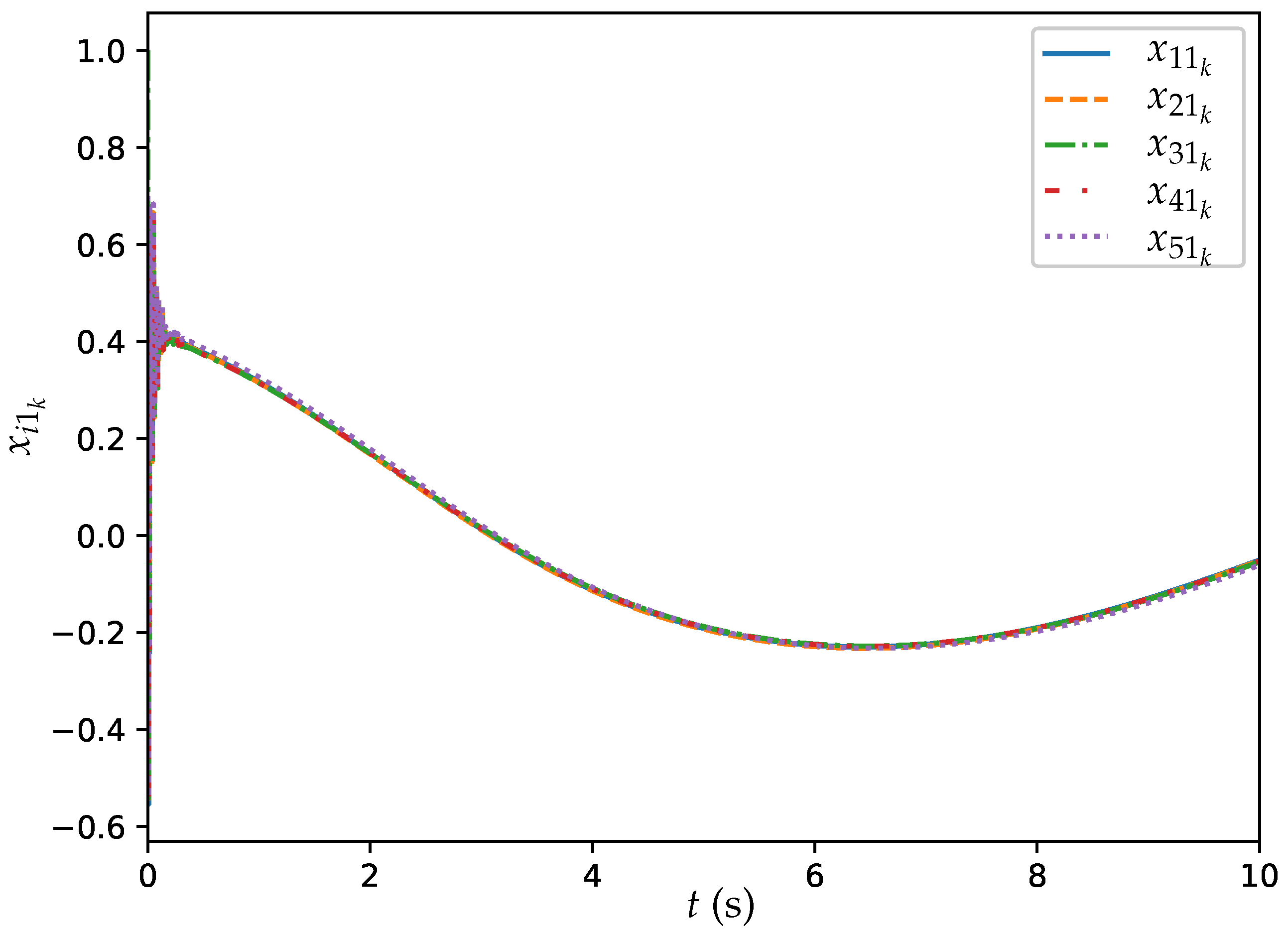
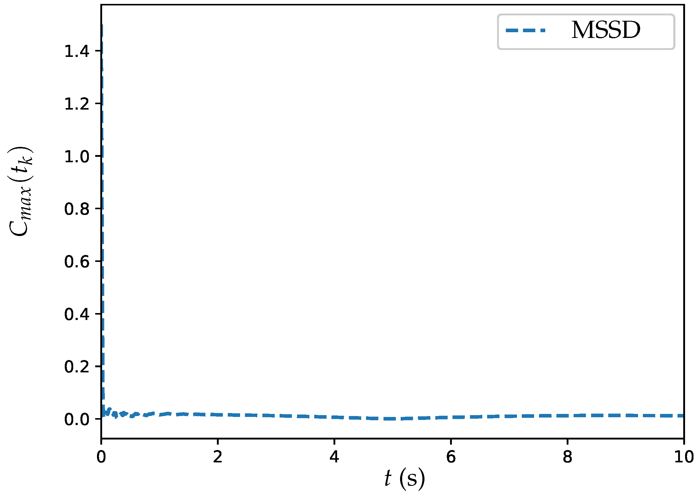
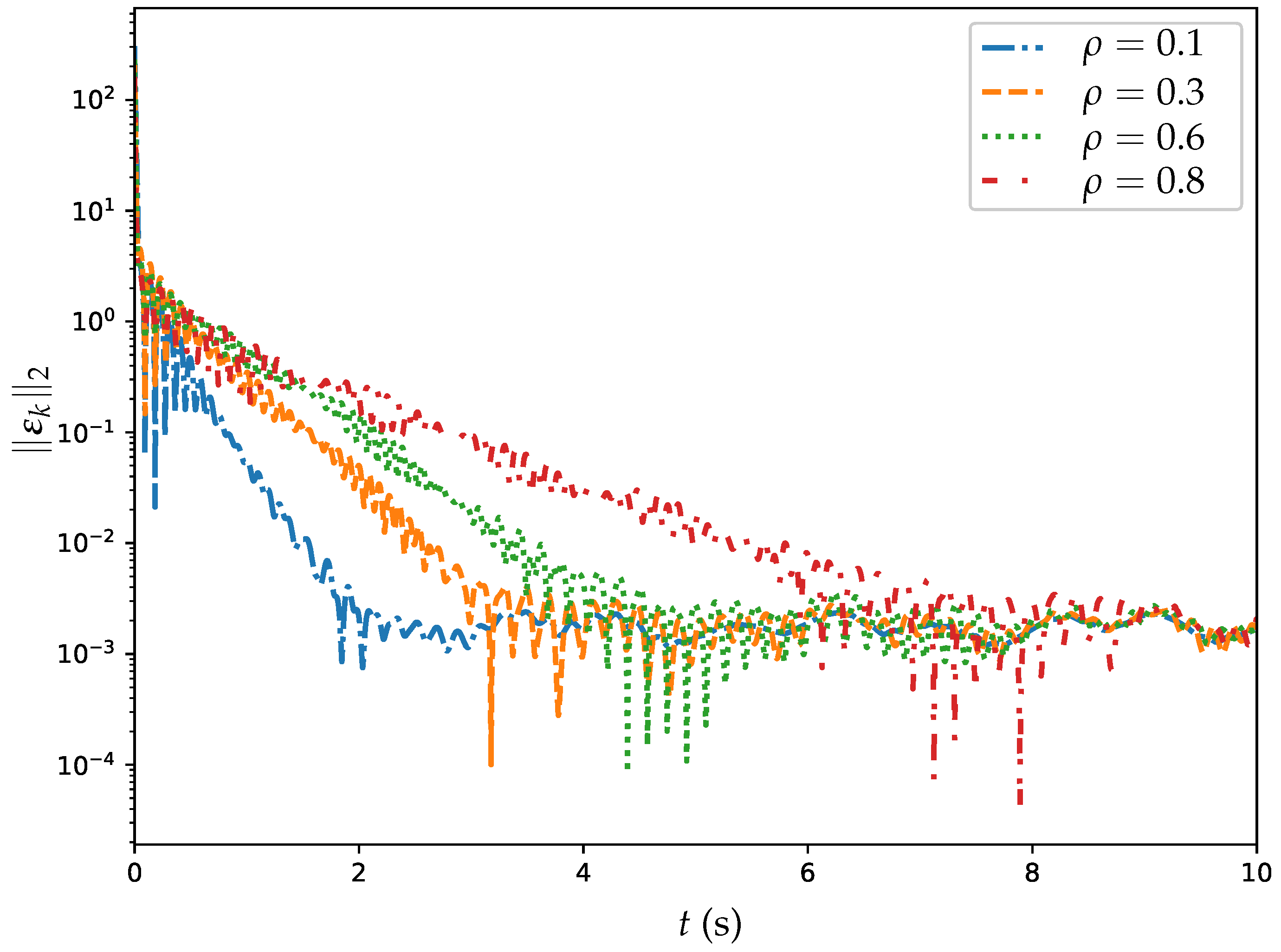
6.1. Example 1: DTDTVO Problem Solved by ET-DTZNN Algorithm

We consider a DTDTVO problem involving a multi-agent system comprising five agents. The DTDTVO problem is formulated as follows:

$$\begin{array}{cc}\hfill \min .& f({\mathbf{x}}_{k+1},t_{k+1})=\sum _{i=1}^5{f}_i(x_{i_{k+1}},t_{k+1}),\hfill \end{array}$$

(27)

where $x_{i_k}\in {\mathbb{R}}^2$. The structure of the network’s communication topology, represented by $\mathcal{G}$, is presented in Figure 1, illustrating the connections among the agents. Detailed time-varying local objective functions $f_i$ for each agent are provided in Table 1.

Figure 1. Communication topology graph $\mathcal{G}$ of multi-agent system in Examples 1 and 2.

Table 1. Expressions of time-varying objective functions in Example 1.

${\mathit{f}}_{\mathit{i}}({\mathit{x}}_{{\mathit{i}}_{{\mathit{t}}_{\mathit{k}}}},{\mathit{t}}_{\mathit{k}})$	Expression
$f_1(x_{1_{t_k}},t_k)$	$sin(0.1t_k-2)x_{{11}_{t_k}}^2/4+x_{{12}_{t_k}}^2+cos(0.1t_k-2)x_{{11}_{t_k}}{x}_{{12}_{t_k}}$
$f_2(x_{2_{t_k}},t_k)$	$x_{{21}_{t_k}}^2+sin(0.1t_k-2)x_{{22}_{t_k}}^2/4+cos(0.3t_k-2)x_{{21}_{t_k}}$
$f_3(x_{3_{t_k}},t_k)$	$x_{{31}_{t_k}}^2+x_{{32}_{t_k}}^2+sin(3t_k-2)x_{{32}_{t_k}}$
$f_4(x_{4_{t_k}},t_k)$	$x_{{41}_{t_k}}^4+cos(0.2t_k-2)x_{{42}_{t_k}}^2+sin(0.3t_k-2)x_{{42}_{t_k}}$
$f_5(x_{5_{t_k}},t_k)$	$cos(0.2t_k-2)x_{{51}_{t_k}}^2+x_{{52}_{t_k}}^4+sin(0.3t_k-2)x_{{51}_{t_k}}$

Prior to the experiment, the parameters of ET-DTZNN Algorithm (22) need to be appropriately set. The operation duration is defined as $T=10$ s, with a sampling interval $\tau$ of $0.001$ s and parameter h configured at $0.3$. For the penalty function, $\sigma$ is assigned a value of 50. Furthermore, the initial states $x_{i_0}$ are randomly initialized within the range $x_{i{j}_0}\in [-1,1]$. The experimental results are showcased in Figure 2, Figure 3, Figure 4 and Figure 5.

Figure 2. Trajectories of $x_{i{1}_k}$ for all agents synthesized by ET-DTZNN algorithm with $\tau =0.001$ s and $\rho =0.6$.

Figure 3. Trajectories of $x_{i{2}_k}$ for all agents synthesized by ET-DTZNN algorithm with $\tau =0.001$ s and $\rho =0.6$.

Figure 4. Trajectory of MSSD $C_{max}\left(t_k\right)$ for ET-DTZNN algorithm when solving DTDTVO problem with $\rho =0.6$, $\sigma =50$, and $\tau =0.001$ s.

Figure 5. Trajectories of MSSRE $\parallel {\mathbf{\epsilon }}_k{\parallel }_2$ for ET-DTZNN algorithm when solving DTDTVO problem with $\rho =0.6$ and different $\tau$.

Figure 2 and Figure 3 illustrate the trajectories of $x_{i{1}_k}$ and $x_{i{2}_k}$ for all agents synthesized by ET-DTZNN Algorithm (22) with $\tau =0.001$ s and $\rho =0.6$. The figure includes five different trajectories, each represented by a different colored dashed line: $x_{1_k}$(blue), $x_{2_k}$ (orange), $x_{3_k}$(green), $x_{4_k}$ (red), and $x_{5_k}$ (purple). The experimental results depicted in Figure 2 and Figure 3 illustrate the effectiveness of ET-DTZNN Algorithm (22) in achieving convergence and consensus for all agents. At the beginning of the simulation, all trajectories exhibit some initial oscillations as the agents adjust their states based on the event-triggered conditions and local objective functions. Over time, the trajectories of all agents converge to a steady state, indicating that ET-DTZNN Algorithm (22) successfully computes the optimal solutions for the time-varying objective functions.

Since achieving consensus is a central aspect of distributed optimization, a specific metric that captures the degree of consensus among the agents over time is introduced. Let us define the maximum steady-state deviation (MSSD) as $C_{max}\left(t_k\right)={max}_{i,j\in \{1,2,\dots n\}}{\parallel x_{i_k}-x_{j_k}\parallel }_2$. The corresponding trajectory of MSSD is illustrated in Figure 4. From Figure 4, it is evident that the MSSD swiftly declines to nearly zero within the initial 2 s, showcasing the algorithm’s capability to effectively achieve consensus. This swift convergence highlights the capability of the ET-DTZNN algorithm to minimize state deviations across agents, ensuring they collaboratively reach a unified solution for the DTDTVO problem efficiently.

Additionally, several experiments are conducted with ET-DTZNN Algorithm (22) solving the DTDTVO problem with different $\tau$. The MSSRE for the whole system is defined as $\parallel {\mathbf{\epsilon }}_k{\parallel }_2={\sum }_{i=1}^5{\parallel {\mathbf{\epsilon }}_{i_k}\parallel }_2$. The corresponding trajectories of MSSREs $\parallel {\mathbf{\epsilon }}_k{\parallel }_2$ are presented in Figure 5 and Table 2.

Table 2. MSSREs of ET-DTZNN algorithm when solving DTDTVO problem with different $\tau$.

$\mathit{\tau }$	MSSRE $\parallel {\mathit{\epsilon }}_{\mathit{k}}{\parallel }_2$
0.001 s	$7.71\times {10}^{-3}$
0.0005 s	$5.81\times {10}^{-4}$
0.0001 s	$6.49\times {10}^{-5}$

In Figure 5, the MSSREs $\parallel {\mathbf{\epsilon }}_k{\parallel }_2$ are shown for various values of $\tau$. The figure illustrates three distinct trajectories: the blue dashed line represents a sampling interval of $\tau =0.001$ s, the orange dashed line corresponds to $\tau =0.0005$ s, and the green dashed line indicates $\tau =0.0001$ s. For $\tau =0.001$ s, the MSSRE decreases from approximately ${10}^2$ to about ${10}^{-3}$, represented by the blue dashed line. For $\tau =0.0005$ s, the MSSRE shows faster convergence, reducing to ${10}^{-4}$, and it is represented by the orange dashed line. The green dashed line, which corresponds to $\tau =0.0001$ s, indicates the most rapid decrease, with the MSSRE reducing from ${10}^2$ to ${10}^{-5}$, highlighting the improved precision achieved with smaller time steps. The figure reveals an evident pattern: a decrease in $\tau$ leads to a reduction in MSSRE, highlighting improved performance of the algorithm when smaller $\tau$ values are utilized. From Figure 5 and Table 3, it can be observed that the MSSRE $\parallel {\mathbf{\epsilon }}_k{\parallel }_2$ follows an order of $O\left({\tau }^2\right)$, which is consistent with and validates the theoretical analyses. It is worth pointing out that an MSSRE of ${10}^{-3}$ is acceptable for applications like robotic coordination, where errors below ${10}^{-2}$ are typically sufficient, whereas energy networks often demand stricter accuracy, such as ${10}^{-4}$ or lower, which we achieve with smaller $\tau$ (e.g., MSSRE of ${10}^{-5}$ at $\tau =0.0001,\mathrm{s}$).

Table 3. Numbers of trigger events of ET-DTZNN algorithm when solving DTDTVO problem with $\tau =0.001$ s and different $\rho$.

Agent	Number of Trigger Events with $\mathit{\rho }=0.1$	Number of Trigger Events with $\mathit{\rho }=0.3$	Number of Trigger Events with $\mathit{\rho }=0.6$	Number of Trigger Events with $\mathit{\rho }=0.8$
Agent 1	1915	1840	1404	1289
Agent 2	5141	1614	1512	1444
Agent 3	4867	1598	1439	1304
Agent 4	6459	2417	2156	1968
Agent 5	6161	2312	2345	2132

In addition, several experiments are conducted with ET-DTZNN Algorithm (22) solving the DTDTVO problem with different $\rho$. The numbers of trigger events for ET-DTZNN Algorithm (22) with different values of $\rho$ for five agents are presented in Figrue Figure 6 and Table 3.

Figure 6. Trajectories of MSSRE $\parallel {\mathbf{\epsilon }}_k{\parallel }_2$ for ET-DTZNN algorithm when solving DTDTVO problem with $\tau =0.001$ s and different $\rho$.

From Table 3, one sees that, for $\rho =0.1$, the number of trigger events is significantly higher for all agents compared with $\rho =0.3$ and $\rho =0.6$. Specifically, Agent 4 has the highest number of trigger events with 6459, followed by Agent 5 with 6161 and Agent 2 with 5141. As $\rho$ increases to 0.3, the number of trigger events decreases for all agents, indicating that a higher $\rho$ value leads to fewer trigger events. This trend continues as $\rho$ increases to 0.6, with the number of trigger events further decreasing for all agents. Agent 4 still has the highest number of trigger events at 2417 for $\rho =0.3$ and 2156 for $\rho =0.6$, followed by Agent 5 with 2312 for $\rho =0.3$ and 2345 for $\rho =0.6$. Figure 6 further illustrates the impact of $\rho$ on the convergence rate, showing trajectories of MSSRE $\parallel {\mathbf{\epsilon }}_k{\parallel }_2$ for $\tau =0.001$ s. For $\rho =0.1$, the convergence rate is the fastest, reaching a low MSSRE within approximately 2 s, while for $\rho =0.3$ and $\rho =0.6$, the convergence slows, taking around 3 and 4 s, respectively. At $\rho =0.8$, the convergence rate is significantly slower, requiring over 6 s to reach a similar MSSRE. This highlights that a smaller $\rho$ accelerates convergence by triggering more frequent updates. However, there is a diminishing return in balancing communication cost and convergence rate; for example, when $\rho =0.8$, the communication cost (number of trigger events) does not reduce significantly compared to $\rho =0.6$—e.g., Agent 4 has 1968 triggers at $\rho =0.8$ versus 2156 at $\rho =0.6$—but the convergence rate is much slower, taking over 6 s compared to 4 s for $\rho =0.6$. The results showcase that the ET-DTZNN algorithm effectively reduces the number of trigger events as $\rho$ increases, highlighting its efficiency in minimizing communication consumption, though at the cost of slower convergence for larger $\rho$ values.

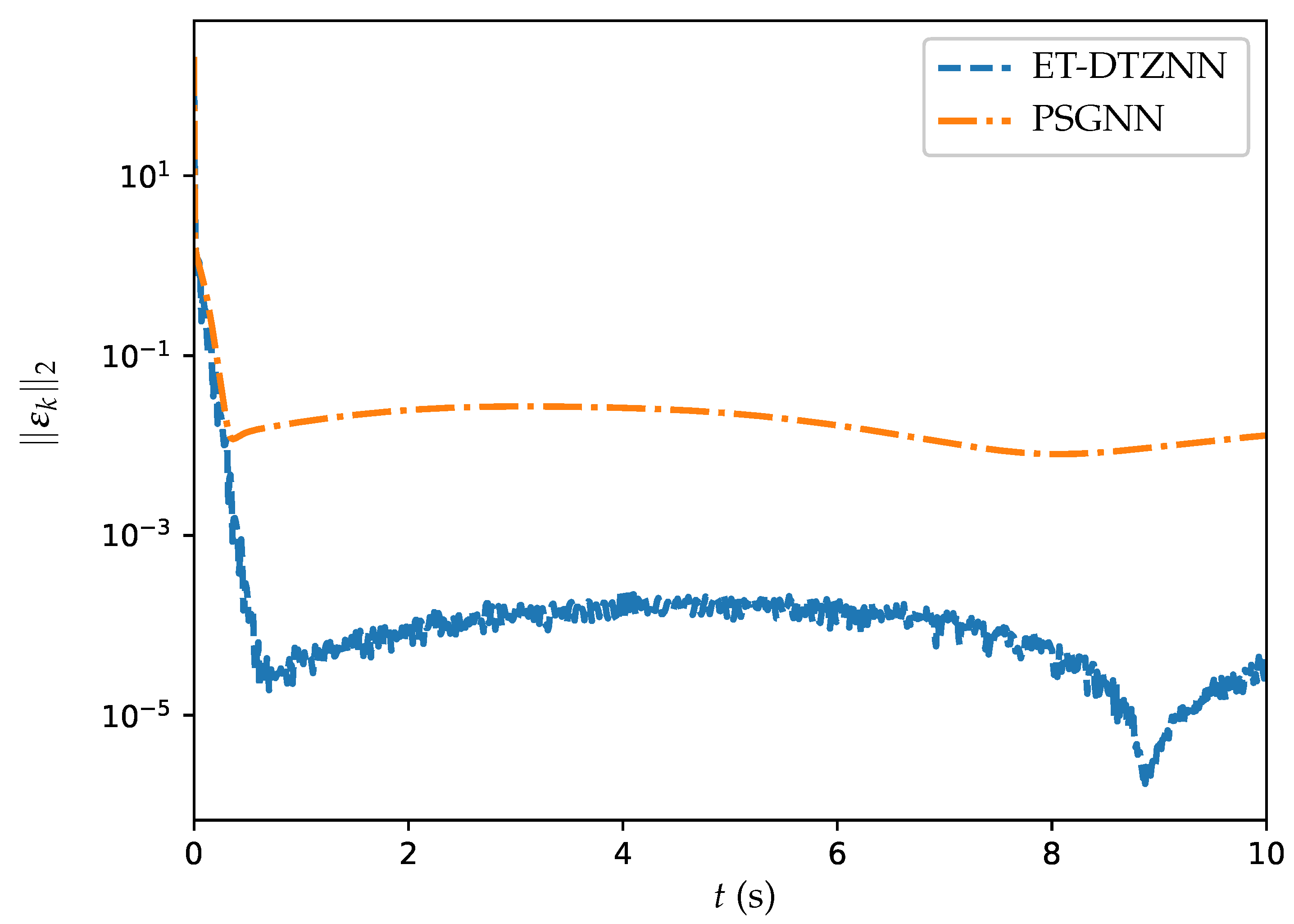
6.2. Example 2: Comparative Experiments

The widely used gradient neural network algorithm addresses time-varying problems effectively. In this subsection, a comparative experiment is performed to evaluate the GNN-based algorithm against the proposed ET-DTZNN algorithm.

First, based on the algorithm presented in [34], a periodic sampling GNN (PSGNN) algorithm is developed to address the DTDTVO problem. Under the PSGNN algorithm, agents periodically exchange their information with neighboring agents at time intervals given by $t_k=k\tau$. For agent i, the scalar-valued energy function is expressed as

$${\mu }_{i_k}={\displaystyle \frac{1}{2}}{\parallel {\mathbf{\epsilon }}_{i_k}\parallel }_2^2,$$

(28)

where ${\mathbf{\epsilon }}_{i_k}=\nabla f_i(x_k,t_k)+\sigma {\sum }_{j\in {\mathcal{N}}_i}(x_{i_k}-x_{j_k})=\nabla f_i(x_k,t_k)+\sigma d_i{x}_{i_k}-\sigma e_{i_k}$. By utilizing the gradient information of Energy Function (28), the following expression is derived:

$$\begin{array}{cc}\hfill {\dot{x}}_{i_k}& =-{\gamma }^G{\displaystyle \frac{\partial {\mu }_{i_k}}{\partial x_{i_k}}}\hfill \\ \hfill & =-{\gamma }^G{\left({\displaystyle \frac{\partial {\mathbf{\epsilon }}_{i_k}}{\partial x_{i_k}}}\right)}^{\mathrm{T}}{\mathbf{\epsilon }}_{i_k}\hfill \\ \hfill & =-{\gamma }^G{(H_{i_k}+d_i\sigma I)}^{\mathrm{T}}{\mathbf{\epsilon }}_{i_k}\hfill \\ \hfill & =-{\gamma }^G{J}_{i_k}^{\mathrm{T}}(\nabla f_i(x_k,t_k)+\sigma d_i{x}_{i_k}-\sigma e_{i_k}),\hfill \end{array}$$

where the parameter ${\gamma }^G$ scales the convergence rate of the GNN algorithm [3]. Thus, the PSGNN algorithm for addressing the DTDTVO problem is defined as

$$x_{i_{k+1}}=x_{i_k}-\tau {\gamma }^G{J}_{i_k}^{\mathrm{T}}(\nabla f_i(x_k,t_k)+\sigma d_i{x}_{i_k}-\sigma e_{i_k}).$$

(29)

Subsequently, both PSGNN and ET-DTZNN algorithms are applied to address the DTDTVO problem. To ensure a fair comparison, the parameter $\sigma$ and the initial states are kept consistent with those defined in Section 6.1, while parameters $\gamma$ and ${\gamma }^G$ are set to $\gamma ={\gamma }^G=3000$. The resulting experimental outcomes are displayed in Table 4 and Figure 7, which provide a detailed comparison of the performance of the PSGNN algorithm and the ET-DTZNN algorithm for solving the DTDTVO problem.

Table 4. MSSREs of PSGNN and ET-DTZNN algorithms in solving DTDTVO problem with $\gamma ={\gamma }^G$ and different values of $\tau$.

$\mathit{\tau }$	MSSRE $\parallel {\mathit{\epsilon }}_{\mathit{k}}{\parallel }_2$ of PSGNN	MSSRE $\parallel {\mathit{\epsilon }}_{\mathit{k}}{\parallel }_2$ of ET-DTZNN
0.001 s	$4.21\times {10}^{-1}$	$7.71\times {10}^{-3}$
0.0005 s	$1.15\times {10}^{-1}$	$5.81\times {10}^{-4}$
0.0001 s	$2.19\times {10}^{-2}$	$6.49\times {10}^{-5}$

Figure 7. Trajectories of MSSREs $\parallel {\mathbf{\epsilon }}_k{\parallel }_2$ for PSGNN and ET-DTZNN algorithms when solving DTDTVO problem with $\rho =0.6$ and $\tau =0.0001$ s.

Figure 7 illustrates the trajectories of the MSSRE $\parallel {ϵ}_k{\parallel }_2$ over time t for two different algorithms: PSGNN and ET-DTZNN. The y-axis represents $\parallel {ϵ}_k{\parallel }_2$ on a logarithmic scale, ranging from ${10}^{-5}$ to ${10}^2$. The blue dashed line represents the ET-DTZNN algorithm, which shows a rapid decrease in $\parallel {ϵ}_k{\parallel }_2$ initially, stabilizing around ${10}^{-5}$. This indicates that the ET-DTZNN algorithm quickly reduces the residual errors and maintains a low error level throughout the experiment. On the other hand, the orange dash–dot line represents the PSGNN algorithm, which shows a slower decrease in $\parallel {ϵ}_k{\parallel }_2$ and stabilizes around ${10}^{-2}$. This indicates that the PSGNN algorithm requires more time to decrease the residual errors and sustains a higher level of error when compared to the ET-DTZNN algorithm. Overall, the ET-DTZNN algorithm presents superior performance in terms of convergence rate and accuracy compared with the PSGNN algorithm. The analysis showcases the success of the ET-DTZNN algorithm in addressing the DTDTVO problem under the configuration of $\rho =0.6$ and $\tau =0.0001$ s, highlighting its efficiency and precision.

Table 4 presents the MSSREs of the PSGNN and ET-DTZNN algorithms in solving the DTDTVO problem with different values of $\tau$. From Table 4, it is observed that as the value of $\tau$ decreases, the MSSRE values for both algorithms also decrease. Specifically, for $\tau =0.001$ s, the MSSRE of PSGNN algorithm is $4.21\times {10}^{-1}$ and the MSSRE of ET-DTZNN algorithm is $7.71\times {10}^{-3}$. For $\tau =0.0005$ s, the MSSRE of PSGNN algorithm is $1.15\times {10}^{-1}$ and the MSSRE of ET-DTZNN algorithm is $5.81\times {10}^{-4}$. Finally, for $\tau =0.0001$ s, the MSSRE of PSGNN algorithm is $2.19\times {10}^{-2}$ and the MSSRE of ET-DTZNN algorithm is $6.49\times {10}^{-5}$. Overall, the ET-DTZNN algorithm consistently outperforms the PSGNN algorithm in terms of precision across all tested $\tau$ values. The results highlight the superior performance of the ET-DTZNN algorithm in achieving more accurate solutions compared with the PSGNN algorithm.

6.3. Example 3: DTDTVO Problem Solved by ET-DTZNN Algorithm in Large MASs

In this subsection, two experiments employ the ET-DTZNN algorithm to tackle a DTDTVO problem within a large MAS under static and dynamic topology, respectively. We consider a DTDTVO problem involving a MAS with 20 agents. The DTDTVO problem is formulated as follows:

$$\begin{array}{cc}\hfill \min .& f({\mathbf{x}}_{k+1},t_{k+1})=\sum _{i=1}^{20}{f}_i(x_{i_{k+1}},t_{k+1}),\hfill \end{array}$$

(30)

where $x_{i_k}\in {\mathbb{R}}^2$. Each agent i ($i=1,\dots ,20$) possesses a local time-varying objective function $f_i(x_{i_k},t_k)=a_{i1}\left(t_k\right)x_{i{1}_k}^2+a_{i2}\left(t_k\right)x_{i{2}_k}^2+b_{i1}\left(t_k\right)x_{i{1}_k}+b_{i2}\left(t_k\right)x_{i{2}_k}$, where $x_{i_k}={[x_{i{1}_k},x_{i{2}_k}]}^{\mathrm{T}}\in {\mathbb{R}}^2$. The coefficients are $a_{i1}\left(t_k\right)=0.5+0.2sin(t_k+0.1i)$, $a_{i2}\left(t_k\right)=0.5+0.2cos(t_k+0.1i)$, $b_{i1}\left(t_k\right)=cos(2t_k+0.1i)$, and $b_{i2}\left(t_k\right)=sin(2t_k+0.1i)$, rendering the functions time-varying and distinct with a phase difference of 0.1 radians between consecutive agents.

Before the experiment begins, it is essential to configure the parameters of the ET-DTZNN algorithm properly. In both static and dynamic topology scenarios, the total operation duration is set at $T=10$ s, with parameter h defined as $0.3$ and $\rho$ assigned a value of $0.2$. Due to the scale of the multi-agent system (MAS), the penalty function parameter $\sigma$ is assigned a value of 200. Additionally, the initial states $x_{i_0}$ are randomly generated within the range of $x_{i{j}_0}\in [-1,1]$.

6.3.1. ET-DTZNN in Large MAS Under Static Topology

Under the static topology, the agents are linked via a ring-shaped communication topology, enabling each agent i to exchange information bidirectionally with neighbors $(i-1)$ and $(i+1)$. The adjacency matrix A assigns $A_{i,j}=1$ for $j=(i\pm 1)$ and 0 otherwise, with degree matrix $D_{i,i}=2$ and Laplacian $L=D-A$, ensuring network connectivity for distributed consensus. The experimental results are illustrated through Figure 8, Figure 9 and Figure 10.

Figure 8. Trajectories of $x_{1k}$ for all agents synthesized by ET-DTZNN algorithm when solving DTDTVO problem within 20 agents under the static topology with $\tau =0.01$ s.

Figure 9. Trajectories of $x_{2k}$ for all agents synthesized by ET-DTZNN algorithm when solving DTDTVO problem within 20 agents under static topology with $\tau =0.01$ s.

Figure 10. Trajectories of MSSREs $\parallel {\mathbf{\epsilon }}_k{\parallel }_2$ for ET-DTZNN algorithm when solving DTDTVO problem within 20 agents under static topology.

Figure 8 and Figure 9 illustrate the trajectories of $x_{i{1}_k}$ and $x_{i{2}_k}$ for all agents under static topology synthesized by ET-DTZNN Algorithm (22) with $\tau =0.01$ s and $\rho =0.2$. The experimental findings, as shown in Figure 8 and Figure 9, demonstrate the capability of the ET-DTZNN algorithm to ensure both convergence and consensus across all agents within a large MAS. At the beginning of the simulation, all trajectories exhibit some initial deviations as the agents adjust their states based on the event-triggered conditions and local objective functions. As time progresses, the trajectories of all agents gradually stabilize, demonstrating the capability of the ET-DTZNN algorithm to effectively resolve the DTDTVO problem in large multi-agent systems.

Additionally, experiments are conducted with the ET-DTZNN algorithm solving the DTDTVO problem in a large MAS with different $\tau$. Figure 10 showcases a semi-log plot illustrating the MSSRE $\parallel {\mathbf{\epsilon }}_k{\parallel }_2$ over a 10-second interval for the ET-DTZNN algorithm addressing a DTDTVO problem with 20 agents. This plot compares the results of two trials, where $\tau =0.01$ s is represented by the blue dashed line and $\tau =0.001$ s is depicted by the orange dotted line. The results show that the smaller sampling interval ($\tau =0.001$ s) yields a low MSSRE of ${10}^{-3}$, while $\tau =0.01$ s exhibits periodic oscillations peaking at ${10}^{-1}$, driven by the time-varying objective function, confirming the theoretical MSSRE scaling of $O\left({\tau }^2\right)$.

6.3.2. ET-DTZNN in Large MAS Under Dynamic Topology

Under the dynamic topology, the agents are linked via a time-varying communication structure, where the topology switches every 1 s to a new randomly generated strongly connected undirected graph. At each switching instant, the adjacency matrix A is constructed using an Erdos–Rényi random graph model with a connection probability of 0.3 [31], ensuring bidirectional information exchange between connected agents. The generation process guarantees strong connectivity by verifying that the resulting graph allows a path between any pair of agents i and j in both directions when considered as a directed graph. This dynamic, strongly connected topology ensures network adaptability and persistent consensus capability despite frequent structural changes. The experimental results are illustrated through Figure 11, Figure 12 and Figure 13.

Figure 11. Trajectories of $x_{1k}$ for all agents synthesized by ET-DTZNN algorithm when solving DTDTVO problem within 20 agents under dynamic topology with $\tau =0.01$ s.

Figure 12. Trajectories of $x_{2k}$ for all agents synthesized by ET-DTZNN algorithm when solving DTDTVO problem within 20 agents under dynamic topology with $\tau =0.01$ s.

Figure 13. Trajectories of MSSREs $\parallel {\mathbf{\epsilon }}_k{\parallel }_2$ for ET-DTZNN algorithm when solving DTDTVO problem within 20 agents under dynamic topology.

Figure 11 and Figure 12 illustrate the trajectories of $x_{i{1}_k}$ and $x_{i{2}_k}$ for all agents synthesized by ET-DTZNN Algorithm (22) under dynamic topology with $\tau =0.01$ s and $\rho =0.2$. The experimental results depicted in Figure 11 and Figure 12 illustrate the effectiveness of the ET-DTZNN algorithm in achieving convergence and consensus for all agents in a large MAS under dynamic topology. The dynamic topology introduces noticeable perturbations at each switching instant (e.g., at $t=1,2,3,\dots$), manifesting as slight discontinuities or oscillations in the trajectories. These perturbations are more pronounced in the early stages when the states are farther apart but diminish as consensus is approached, indicating the robustness of the ET-DTZNN algorithm to topological changes. The impact of the dynamic topology is evident in the small, periodic deviations from smooth convergence, yet the algorithm maintains overall stability and achieves consensus, highlighting its adaptability to frequent structural changes in the communication network.

Additionally, experiments are conducted with the ET-DTZNN algorithm solving the DTDTVO problem in a large MAS with different $\tau$. Figure 13 displays a semi-log plot illustrating the MSSRE $\parallel {\mathbf{\epsilon }}_k{\parallel }_2$ over a 10-second interval. This plot evaluates the ET-DTZNN algorithm’s performance in solving a DTDTVO problem with 20 agents under dynamic topology. Two trials are compared, with the blue dashed line representing $\tau =0.01$ s and the orange dotted line depicting $\tau =0.001$ s. The MSSRE trajectories demonstrate the algorithm’s convergence despite the dynamic topology, with both experiments showing a rapid initial decrease followed by periodic fluctuations. For $\tau =0.01$ s, the MSSRE drops from ${10}^3$ to around ${10}^1$ within the first second, while for $\tau =0.001$ s, it decreases to around ${10}^{-}1$, reflecting the theoretical $O\left({\tau }^2\right)$ error bound. The dynamic topology introduces noticeable spikes in the MSSRE at each switching instant (e.g., $t=1,2,3,\dots$), as the sudden change in communication structure perturbs the consensus process. These spikes are more pronounced for $\tau =0.01$ s due to the larger sampling interval, which limits the algorithm’s ability to quickly adapt to topological changes. In contrast, the smaller $\tau =0.001$ s, combined with a larger $\gamma$, results in a lower MSSRE and smaller fluctuations, indicating better adaptability to the dynamic topology. Despite these perturbations, the MSSRE remains bounded, underscoring the robustness of ET-DTZNN in handling frequent topological switches while maintaining effective distributed optimization.

It is worth mentioning that the fully distributed nature of the ET-DTZNN algorithm ensures that each agent’s computation time per iteration depends primarily on the size of its local neighborhood rather than the total number of agents in the MAS. As shown in Equation (22), each agent computes its update using only its own objective function and the states of its neighbors, resulting in a computational complexity that scales with degree $d_i$ of the agent in graph G. This design keeps per-agent computation lightweight even as the system size grows. Furthermore, the event-triggered mechanism, governed by the condition in Equation (17), reduces communication overhead by limiting inter-agent exchanges to instances when the local error ${∥{\mathit{\varphi }}_{i_k}∥}_2$ exceeds a threshold relative to ${∥{\mathbf{\epsilon }}_{i_k}∥}_2$. This approach significantly mitigates communication delays, a critical factor in real-time applications, as evidenced by the rapid convergence observed in Figure 8 and Figure 11 across both static and dynamic topologies.

7. Conclusions

To address the DTDTVO problem for MASs characterized by time-varying objective functions, a novel ET-CTZNN model is introduced. This model effectively tackles the CTDTVO problem using a semi-centralized approach. Building upon the ET-CTZNN framework, the ET-DTZNN algorithm is developed. By discretizing the ET-CTZNN model using the Euler formula, the ET-DTZNN algorithm enables agents to compute optimal solutions based on local information and communicate with neighbors only when specific event-triggered conditions are met, significantly reducing communication consumption. For both the ET-CTZNN model and the ET-DTZNN algorithm, their convergence theorems are thoroughly validated. Numerical experiments highlight the effectiveness of the proposed ET-DTZNN algorithm, showcasing its precision and enhanced communication efficiency. Looking forward, the ET-DTZNN algorithm shows potential for applications in smart grids, sensor networks, and collaborative robotics, where it can optimize time-varying objectives while minimizing communication. However, the ET-DTZNN algorithm assumes strong convexity of objective functions, uses a static event-triggering threshold, and relies on Euler discretization. Future work may focus on real-world validation to address challenges like distributed non-convex optimization, integrating adaptive event-triggering for better adaptability, and exploring higher-order discretization methods like Runge–Kutta to enhance stability and accuracy.

References

- Patari, N.; Venkataramanan, V.; Srivastava, A.; Molzahn, D.K.; Li, N.; Annaswamy, A. Distributed optimization in distribution systems: Use cases, limitations, and research needs. IEEE Trans. Power Syst. 2022, 37, 3469–3481. [Google Scholar]
- Cavraro, G.; Bolognani, S.; Carli, R.; Zampieri, S. On the need for communication for voltage regulation of power distribution grids. IEEE Trans. Control Netw. Syst. 2019, 6, 1111–1123. [Google Scholar]
- He, L.; Cheng, H.; Zhang, Y. Centralized and decentralized event-triggered Nash equilibrium-seeking strategies for heterogeneous multi-agent systems. Mathematics 2025, 13, 419. [Google Scholar] [CrossRef]
- Molzahn, D.K.; Dorfler, F.; Sandberg, H.; Low, S.H.; Chakrabarti, S.; Baldick, R.; Lavaei, J. A survey of distributed optimization and control algorithms for electric power systems. IEEE Trans. Smart Grid 2017, 8, 2941–2962. [Google Scholar]
- Pan, P.; Chen, G.; Shi, H.; Zha, X.; Huang, Z. Distributed robust optimization method for active distribution network with variable-speed pumped storage. Electronics 2024, 13, 3317. [Google Scholar] [CrossRef]
- Luo, S.; Peng, K.; Hu, C.; Ma, R. Consensus-based distributed optimal dispatch of integrated energy microgrid. Electronics 2023, 12, 1468. [Google Scholar] [CrossRef]
- Tariq, M.I.; Mansoor, M.; Mirza, A.F.; Khan, N.M.; Zafar, M.H.; Kouzani, A.Z.; Mahmud, M.A.P. Optimal control of centralized thermoelectric generation system under nonuniform temperature distribution using barnacles mating optimization algorithm. Electronics 2021, 10, 2839. [Google Scholar] [CrossRef]
- Yang, S.; Shen, Y.; Cao, J.; Huang, T. Distributed heavy-ball over time-varying digraphs with barzilai-borwein step sizes. IEEE Trans. Emerg. Top. Comput. Intell. 2024, 8, 4011–4021. [Google Scholar]
- An, W.; Ding, D.; Dong, H.; Shen, B.; Sun, L. Privacy-preserving distributed optimization for economic dispatch over balanced directed networks. IEEE Trans. Inf. Forensics Secur. 2024, 20, 1362–1373. [Google Scholar]
- Liu, M.; Li, Y.; Chen, Y.; Qi, Y.; Jin, L. A distributed competitive and collaborative coordination for multirobot systems. IEEE Trans. Mobile Comput. 2024, 23, 11436–11448. [Google Scholar]
- Huang, B.; Zou, Y.; Chen, F.; Meng, Z. Distributed time-varying economic dispatch via a prediction-correction method. IEEE Trans. Circuits Syst. I 2022, 69, 4215–4224. [Google Scholar] [CrossRef]
- He, S.; He, X.; Huang, T. A continuous-time consensus algorithm using neurodynamic system for distributed time-varying optimization with inequality constraints. J. Franklin I 2021, 358, 6741–6758. [Google Scholar] [CrossRef]
- Sun, S.; Xu, J.; Ren, W. Distributed continuous-time algorithms for time-varying constrained convex optimization. IEEE Trans. Autom. Control 2023, 68, 3931–3945. [Google Scholar] [CrossRef]
- Zheng, Y.; Liu, Q.; Wang, J. A specified-time convergent multiagent system for distributed optimization with a time-varying objective function. IEEE Trans. Autom. Control 2023, 68, 1590–1605. [Google Scholar] [CrossRef]
- Wang, B.; Sun, S.; Ren, W. Distributed time-varying quadratic optimal resource allocation subject to nonidentical time-varying hessians with application to multiquadrotor hose transportation. IEEE Trans. Syst. Man Cybern. Syst. 2022, 52, 6109–6119. [Google Scholar] [CrossRef]
- Ding, Z. Distributed time-varying optimization—An output regulation approach. IEEE Trans. Cybern. 2024, 54, 1362–1373. [Google Scholar] [CrossRef]
- Rahili, S.; Ren, W. Distributed continuous-time convex optimization with time-varying cost functions. IEEE Trans. Autom. Control 2017, 62, 1590–1605. [Google Scholar] [CrossRef]
- Zhang, Y.; Jiang, D.; Wang, J. A recurrent neural network for solving sylvester equation with time-varying coefficients. IEEE Trans. Neural Netw. 2002, 13, 1053–1063. [Google Scholar] [CrossRef]
- Zhang, Y.; He, L.; Hu, C.; Guo, J.; Li, J.; Shi, Y. General four-step discrete-time zeroing and derivative dynamics applied to time-varying nonlinear optimization. J. Comput. Appl. Math. 2019, 347, 314–329. [Google Scholar] [CrossRef]
- Liao, B.; Han, L.; He, Y.; Cao, X.; Li, J. Prescribed-time convergent adaptive ZNN for time-varying matrix inversion under harmonic noise. Electronics 2022, 11, 1636. [Google Scholar] [CrossRef]
- Zhou, P.; Tan, M.; Ji, J.; Jin, J. Design and analysis of anti-noise parameter-variable zeroing neural network for dynamic complex matrix inversion and manipulator trajectory tracking. Electronics 2022, 11, 824. [Google Scholar] [CrossRef]
- Xiao, L.; Luo, J.; Li, J.; Jia, L.; Li, J. Fixed-time consensus for multiagent systems under switching topology: A distributed zeroing neural network-based method. IEEE Syst. Man Cybern. Mag. 2024, 10, 44–55. [Google Scholar]
- Liao, B.; Wang, T.; Cao, X.; Hua, C.; Li, S. A novel zeroing neural dynamics for real-time management of multi-vehicle cooperation. IEEE Trans. Intell. Veh. 2024, early access, 1–16. [Google Scholar]
- Tan, N.; Yu, P.; Zhong, Z.; Zhang, Y. Data-driven control for continuum robots based on discrete zeroing neural networks. IEEE Trans. Ind. Inform. 2023, 19, 7088–7098. [Google Scholar]
- Jin, L.; Li, S.; Xiao, L.; Lu, R.; Liao, B. Cooperative motion generation in a distributed network of redundant robot manipulators with noises. IEEE Trans. Syst. Man Cybern. Syst. 2018, 48, 1715–1724. [Google Scholar]
- Chen, J.; Pan, Y.; Zhang, Y. ZNN continuous model and discrete algorithm for temporally variant optimization with nonlinear equation constraints via novel td formula. IEEE Trans. Syst. Man Cybern. Syst. 2024, 54, 3994–4004. [Google Scholar]
- Zuo, Q.; Li, K.; Xiao, L.; Wang, Y.; Li, K. On generalized zeroing neural network under discrete and distributed time delays and its application to dynamic Lyapunov equation. IEEE Trans. Syst. Man Cybern. Syst. 2022, 52, 5114–5126. [Google Scholar]
- Dai, J.; Tan, P.; Xiao, L.; Jia, L.; He, Y.; Luo, J. A fuzzy adaptive zeroing neural network model with event-triggered control for time-varying matrix inversion. IEEE Trans. Fuzzy Syst. 2023, 31, 3974–3983. [Google Scholar]
- Kong, Y.; Zeng, X.; Jiang, Y.; Sun, D. A predefined time fuzzy neural solution with event-triggered mechanism to kinematic planning of manipulator with physical constraints. IEEE Trans. Fuzzy Syst. 2024, 32, 4646–4659. [Google Scholar]
- Golub, G.; Loan, C.F. Matrix Computations, 4th ed.; John Hopkins Univesity Press: Baltimore, MD, USA, 2013; pp. 22–33. [Google Scholar]
- Diestel, R. Graph Theory, 5th ed.; Springer: Berlin/Heidelberg, Germany, 2017; pp. 1–33. [Google Scholar]
- Bahman, G.; Jorge, C. Distributed continuous-time convex optimization on weight-balanced digraphs. IEEE Trans. Automat. Contr. 2014, 59, 781–786. [Google Scholar]
- Khalil, H.K. Nonlinear Systems, 3rd ed.; Prentice Hall: Upper Saddle River, NJ, USA, 2002; pp. 111–181. [Google Scholar]
- Zhang, Z.; Yang, S.; Zheng, L. A penalty strategy combined varying-parameter recurrent neural network for solving time-varying multi-type constrained quadratic programming problems. IEEE Trans. Neural Netw. Learn. Syst. 2021, 32, 2993–3004. [Google Scholar]
Disclaimer/Publisher’s Note: The statements, opinions and data contained in all publications are solely those of the individual author(s) and contributor(s) and not of MDPI and/or the editor(s). MDPI and/or the editor(s) disclaim responsibility for any injury to people or property resulting from any ideas, methods, instructions or products referred to in the content. |
© 2025 by the authors. Licensee MDPI, Basel, Switzerland. This article is an open access article distributed under the terms and conditions of the Creative Commons Attribution (CC BY) license (https://creativecommons.org/licenses/by/4.0/).