Article

Hybrid CNN-BiGRU-AM Model with Anomaly Detection for Nonlinear Stock Price Prediction

1
School of Electronic Information and Electrical Engineering, Yangtze University, Jingzhou 434023, China
2
School of Computer Science, Yangtze University, Jingzhou 434023, China
3
School of Mechanical Engineering, Yangtze University, Jingzhou 434023, China
4
School of Computer Science, Central South University, Changsha 410083, China
5
School of Electronic Information, Central South University, Changsha 410004, China
*
Author to whom correspondence should be addressed.
These authors contributed equally to this work.
Electronics 2025, 14(7), 1275; https://doi.org/10.3390/electronics14071275
Submission received: 2 February 2025 / Revised: 7 March 2025 / Accepted: 18 March 2025 / Published: 24 March 2025

Abstract

:
To address challenges in stock price prediction including data nonlinearity and anomalies, we propose a hybrid CNN-BiGRU-AM framework integrated with deep learning-based anomaly detection. First, an anomaly detection module identifies irregularities in stock price data. The CNN component then extracts local features while filtering anomalous information, followed by nonlinear pattern modeling through BiGRU with attention mechanisms. Final predictions undergo secondary anomaly screening to ensure reliability. Experimental evaluation on Shanghai Composite (SSE) daily closing prices demonstrates superior performance with R 2 = 0.9903, RMSE = 22.027, MAE = 19.043, and a Sharpe Ratio of 0.65. It is noteworthy that the MAE of this model is reduced by 14.7%, and the RMSE is decreased by 7.7% compared to its ablation model. The framework achieves multi-level feature extraction through convolutional operations and bidirectional temporal modeling, effectively enhancing model generalization via nonlinear mapping and anomaly correction. Comparative Sharpe Ratio analysis across models provides practical insights for investment decision-making. This dual-functional system not only improves prediction accuracy but also offers interpretable references for market mechanism analysis and regulatory policy formulation.

1. Introduction

Stocks have rapidly gained widespread popularity as they provide investors with a new way to increase their wealth and are considered a barometer of economic and financial activity in a country or region since their first issuance [1,2]. As the stock market continues to grow, it has not only contributed to the growth of the market economy but has also led to the rise of stock price forecasting techniques.
From the early days which relied on fundamental analysis such as financial statements [3] and industry outlook analysis [4] and technical analysis such as K-charts [5] and moving averages [6], to the later introduction of statistical models and quantitative investment strategies such as time series analysis [7] and regression analysis [8], to the introduction of statistical models and quantitative investment strategies [9,10], all of which were not as effective as they could have been. Because stock price forecasting is a nonlinear forecasting task, it generally manifests highly nonlinear characteristics. Price fluctuations are influenced by a multitude of factors, including market sentiment, news events, macroeconomic indicators, etc. These factors may interact with each other in a nonlinear manner [11]. Traditional linear models cannot effectively capture these intricate nonlinear relationships. Later, machine learning algorithms such as logistic regression [12], random forest [13], and support vector machines [14,15] compensate for the shortcomings of traditional stock price forecasting methods when dealing with nonlinear data. However, since most of them are single-model predictions and the methodological principles are slightly backward, they have limitations in terms of prediction accuracy.
In recent years, the development of deep learning techniques has provided new methods for stock price prediction [16,17,18]. Among them, convolutional neural networks (CNNs) are effective in extracting local features from time-series data but lack in capturing long-term dependencies [19,20]. Recurrent neural networks (RNNs), especially long short-term memory (LSTM) networks and gated recurrent units (GRUs), perform well in dealing with long-term dependencies in time series. Yao used the LSTM model to experiment on randomly selected stocks from CSI 300 constituents and found that the prediction results are better than the other two models in comparison, but there is still more valuable information that has not been fully exploited [21]. Researchers have progressively developed prediction models from single-model approaches to hybrid models, which integrate the strengths of various models, resulting in enhanced predictive capabilities [22,23]. For instance, the CNN-LSTM architecture has made significant strides in stock price trend prediction by combining the spatial feature extraction capabilities of convolutional neural networks with the temporal modeling capabilities of long short-term memory networks [24]. Similarly, the Attention-BiLSTM model has improved prediction accuracy by dynamically focusing on key time points through the integration of the attention mechanism [25]. However, existing hybrid models still exhibit significant limitations. The feature fusion mechanism between different modules is relatively simplistic, often relying on direct concatenation or weighted averaging, which fails to fully capture the deep correlations between features [26]. Furthermore, these models are highly dependent on the quality of input data and lack a dynamic evaluation mechanism for assessing data features [27]. These limitations have driven researchers to explore more advanced hybrid model architectures to enhance both the robustness and predictive performance of the models.
Additionally, it is important to note that stock price data may contain anomalies, such as drastic fluctuations triggered by breaking news or market manipulation. Although these anomalies are relatively rare, they cannot be overlooked. Traditional statistical methods face considerable challenges in identifying such anomalies: on the one hand, the scarcity of abnormal samples makes it difficult for models to learn effective discriminative features; on the other hand, the transient nature of abnormal behavior complicates the ability of traditional methods to capture them in a timely manner. Consequently, when confronted with such data, the model may not adjust in time, potentially leading to false or missed anomalies [28,29]. As a result, effectively identifying and processing abnormal data has become a critical challenge in enhancing the robustness of stock price prediction models.
In summary, existing research presents three main limitations: first, traditional prediction methods struggle to adapt to the high-frequency fluctuations and nonlinear dynamics of stock price data; second, mainstream hybrid models have not effectively integrated the synergistic mechanisms of spatiotemporal feature extraction and dynamic anomaly filtering; and third, prediction systems lack the ability to adaptively correct for abnormal interference. These shortcomings contribute to the significant lack of prediction robustness in existing models under complex market conditions.
Based on the above analysis, this paper proposes a hybrid model based on the convolutional neural network, bidirectional gated recurrent unit, and attention mechanism (CNN-BiGRU-AM), and introduces a deep learning-based anomaly detection method. The method first detects anomalies in stock price data with the anomaly detection mechanism; then, extracts local features of the data with a CNN and filters the anomalous information in the features to make nonlinear predictions with the BiGRU-AM model; finally, it detects anomalies in the prediction results to determine whether it is necessary to re-evaluate them.
The innovative design of the method proposed in this paper addresses three core challenges: first, the CNN component tackles the issue of feature extraction from nonlinear patterns in price series by using convolution kernels to capture multi-scale local features; second, the BiGRU component overcomes the limitation of unidirectional information flow in traditional RNNs by employing a bidirectional gating structure, which simultaneously models the influence of both historical and future information on the current data point; third, the AM combined with the autoencoder (AE) module addresses the problem of feature distortion caused by outliers, using attention weights and outlier filtering to dynamically purify the feature space, thereby enhancing the performance and reliability of the prediction model.

2. Methodology

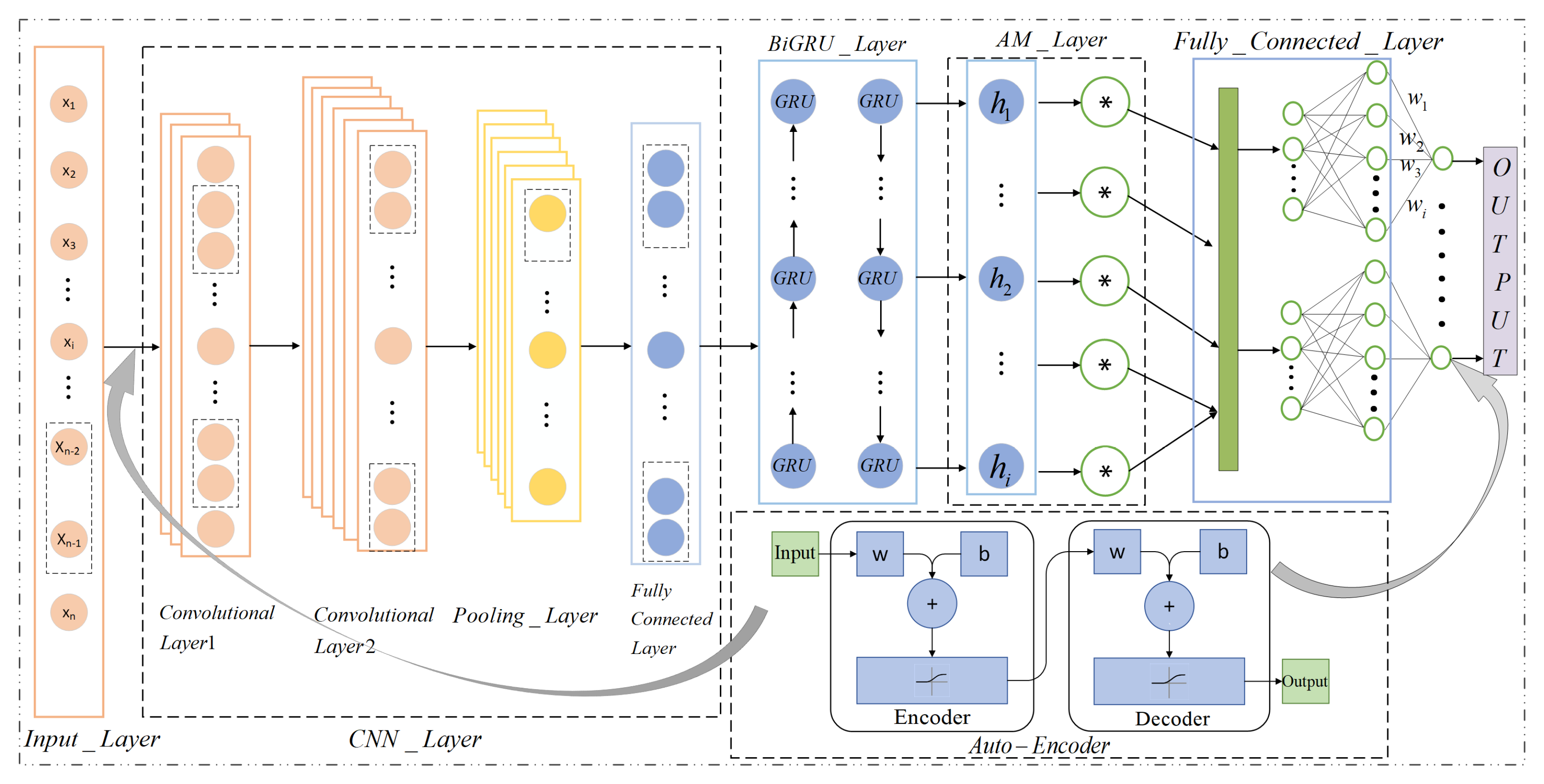
2.1. Overview of the Forecasting Framework

To solve the problem of nonlinearity and anomaly of data in stock price prediction, this study proposes a hybrid model, which incorporates CNN, BiGRU, and an attention mechanism. Additionally, this model incorporates a deep learning-based anomaly detection mechanism. The model initially extracts local features by inputting a convolutional neural network following anomaly detection. It then captures both the long and short-term dependencies of the time series using a bidirectional gated recurrent unit. The model weights important features using an attention mechanism and finally detects anomalies in the data to improve prediction accuracy. The model structure is shown in Figure 1:

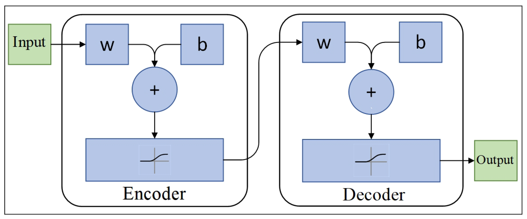
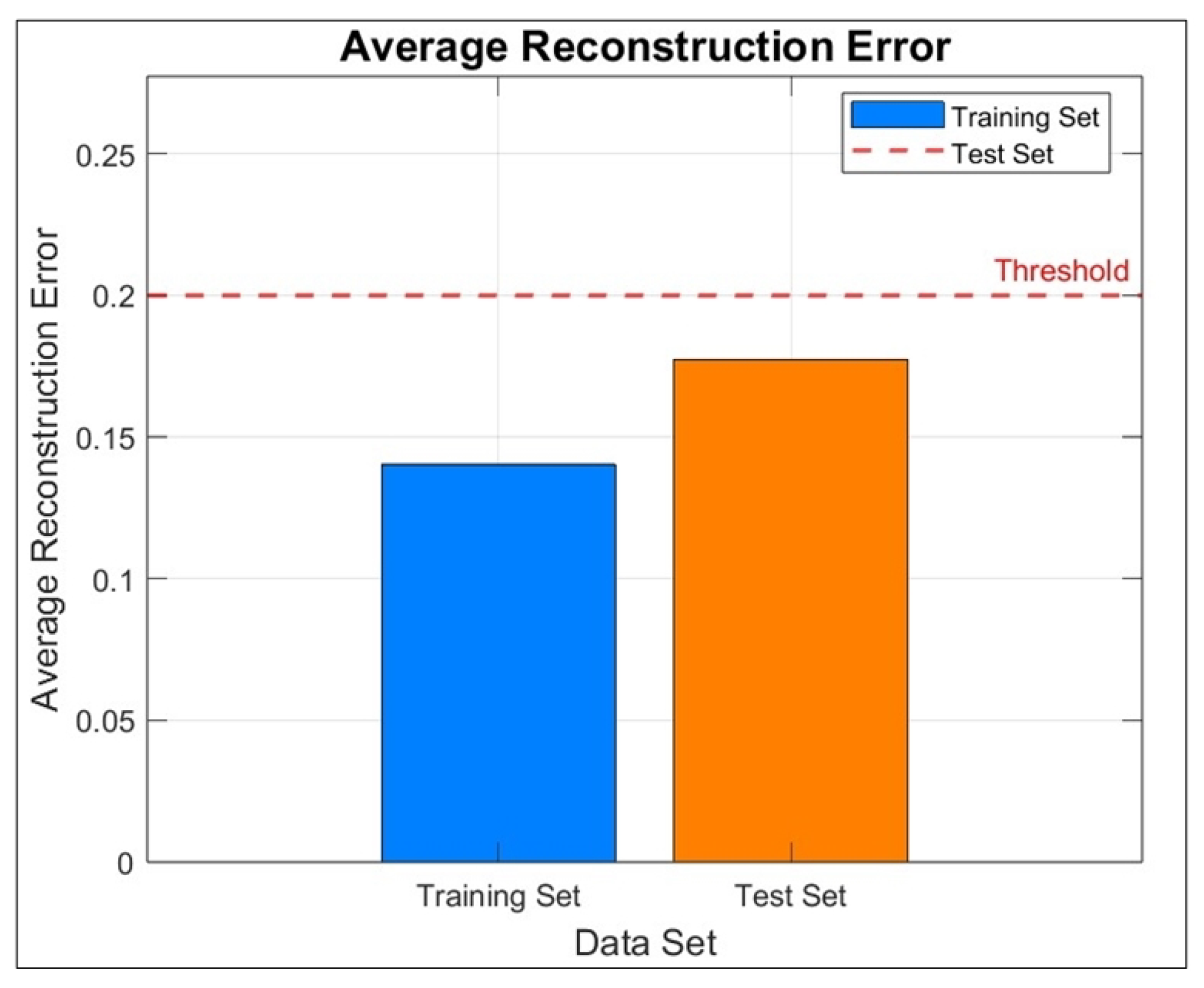
2.2. Auto-Encoder in Anomaly Detection

Auto-encoder is a neural network model employed for unsupervised learning, primarily aimed at learning efficient data representations. The core idea is to train the network to compress the input data into a lower-dimensional representation, which is also called potential space, and then reconstruct the data from this compressed representation.The auto-encoder consists of two main components: one is the encoder, which is responsible for mapping the input data to the latent space, and the decoder, which reconstructs the data from the latent space. Its basic structure is shown in Figure 2:
h = f θ ( X ) = σ ( W X + b )
X R = g ϕ ( h ) = σ ( W h + b )
where X R n is the input data, h R m is the encoded representation, X R R n is the reconstructed output, W and W are the weight matrices of the encoder and decoder, respectively, b and b are the bias terms, and Q is an activation function, and in this paper we use the ReLU function as the activation function.
In the context of anomaly detection, the auto-encoder is trained on normal data. It is assumed that the auto-encoder is able to reconstruct the normal data efficiently, but is less effective in reconstructing the anomalous data, leading to a higher reconstruction error [30]. The fraction of anomalies for a given data point can be defined as its reconstruction error:
the anomaly score = X X R 2
the initial screening of anomalies is conducted expeditiously through the utilization of the percentile method. Following this, an analysis of the data distribution is undertaken to verify the reconstruction error distribution and to select statistical methods or distribution fitting techniques. The next step involves the selection of an appropriate quantile value τ . The final step in the process is to validate and optimize the queues by combining them with standard data τ . If the anomaly score of a new data point exceeds this threshold, the point is classified as an anomaly:
abnormal = 1 , if X X R 2 > τ 0 , else

2.3. Convolutional Neural Network
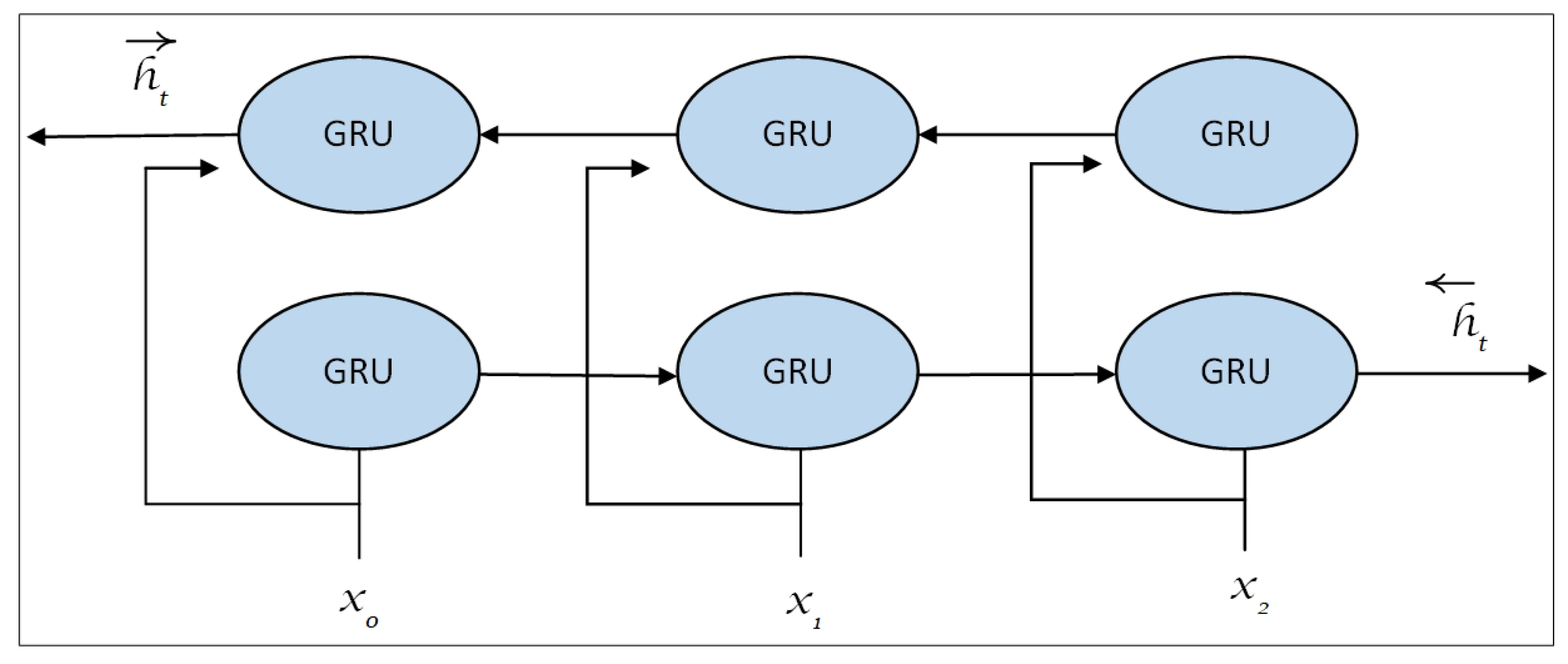
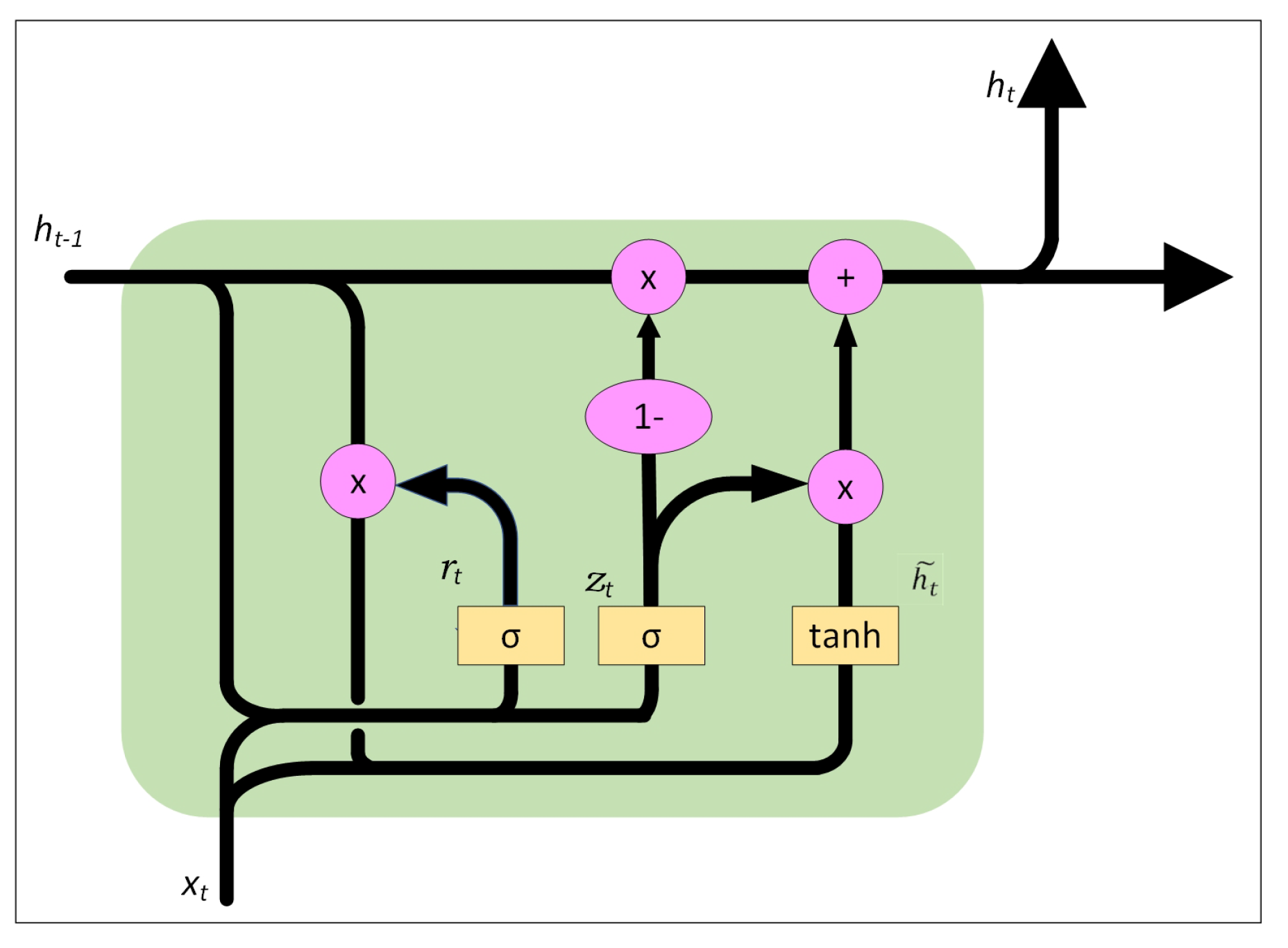
A CNN is a deep learning model. Unlike traditional fully connected neural networks, CNNs can efficiently extract spatial features in images through convolutional operations and pooling operations, thus reducing the number of parameters in the model and improving computational efficiency [31]. As shown in Figure 3, the convolutional layer is one of the core components of the CNN, and its main task is to extract local features by performing convolutional operations on the input data through the convolutional kernel. The extraction of local features, periodic fluctuations, mutations, trends, and other such phenomena contained within the local area is achieved while concomitantly reducing the amount of computation. Concurrently, the convolution operation enables the model to concentrate on local salient features, thereby reducing interference from irrelevant parts and facilitating the model’s comprehension of the local and global structure of the data. Given the input image X and the convolution kernel W, the output Y of the convolution operation can be expressed as follows:
Y i , j = ( X W ) i , j = m n X i + m , j + n · W m , n
where ∗ is the convolution operation, i , j is the coordinates of the output feature map, and m , n is the coordinates of the convolution kernel. After the convolution layer, a nonlinear activation function is usually applied to introduce nonlinear properties of the model. The activation function used in this paper is the ReLU function:
ReLU ( x ) = max ( 0 , x )
which is selected due to its efficacy in addressing the gradient vanishing issue while maintaining computational simplicity [32].
The convolutional layer is followed by a pooling layer, which is typically employed to downsample the output of the convolutional layer with the objective of reducing the size of the feature map and consequently reducing the computational complexity. Common pooling methods include Max Pooling and Average Pooling, the former of which is utilized in this paper. Taking the maximum pooling of m × m as an illustrative example, the pooling operation can be expressed as follows:
Y i , j = max { X m i , m j , X m i , m j + 1 , X m i + 1 , m j , X m i + 1 , m j + 1 }
The pooling layer can effectively reduce the size of the feature map while retaining important spatial information [33]. After multiple layers of convolution and pooling operations, the feature map is usually spread into a vector and passed into the fully connected layer for further classification or regression tasks. The computation of the fully connected layer can be represented as follows:
y = W · x + b
where x is the input vector, W is the weight matrix, b is the bias vector, and y is the output. CNN can effectively extract and utilize the hierarchical features in the input data and output data through the above hierarchical structure.

2.4. BiGRU Model

The BiGRU is an enhanced RNN model, as illustrated in Figure 4, which integrates two GRU networks, forward and backward, to more effectively capture contextual information in sequence data [34]. In contrast to conventional unidirectional GRUs, whose structure is shown in Figure 5, the BiGRU can contemplate both the preceding and subsequent information of the input sequences, thereby enhancing the model’s capacity to model time-series data.
The GRU is a simplified version of a (LSTM) network. It controls the flow of information through two gating mechanisms, namely the update gate and the reset gate [35]. Given the input t at time step x t and the hidden state h t 1 at the previous time step, the GRU unit is computed as follows:
z t = σ ( W z · x t + U z · h t 1 + b z )
r t = σ ( W r · x t + U r · h t 1 + b r )
h ˜ t = tanh ( W h · x t + r t ( U h · h t 1 ) + b h )
h t = ( 1 z t ) h t 1 + z t h ˜ t
where z t denotes the update gate, r t denotes the reset gate, h ˜ t denotes the candidate hidden state, h t denotes the final hidden state, σ denotes the sigmoid activation function, tanh denotes the hyperbolic tangent activation function, and ∘ denotes the element-by-element product.
Bidirectional GRUs process input sequences by introducing a forward GRU and a reverse GRU simultaneously. These two GRU units process the forward-backward and backward-forward sequences, respectively, and subsequently merge their hidden states as follows:
h t = GRU forward ( x t , h t 1 )
h t = GRU backward ( x t , h t + 1 )
The GRU formula in Equations (13) and (14) corresponds to Equations (9)–(12).
The final output is as follows:
h t = [ h t ; h t ]
This above-mentioned structure enables BiGRU to simultaneously consider the information present before and after the sequence at each time step, thereby enhancing the ability to capture complex temporal patterns [36].

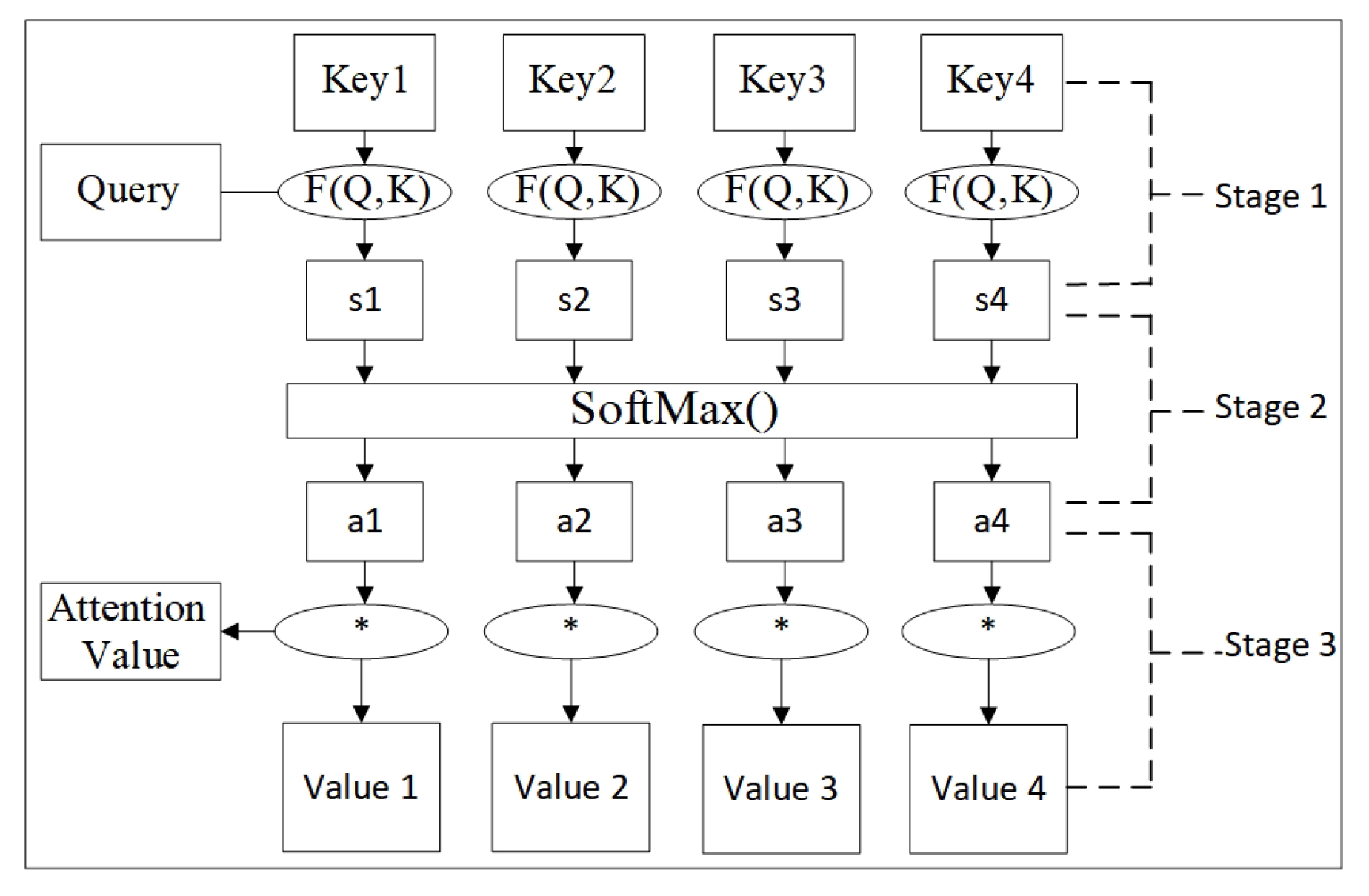
2.5. Attention Mechanism

As is shown in Figure 6, the AM is a technique that is widely employed in deep learning models. The technique improves the performance of a model by assigning different weights to different parts of the input sequence, thereby enabling the model to focus more effectively on important information [37]. The fundamental aspect of the AM is the calculation of attention weights, which are utilized to quantify the influence of each element within the input sequence on the output. When a query vector, denoted by q , a key vector, represented by k , and a value vector, represented by v , are provided, the attention score is typically computed by
score ( q , k ) = q k
In order to obtain the attention weight α i , the score is normalized using the Softmax function:
α i = exp ( score ( q , k i ) ) j exp ( score ( q , k j ) )
The final output of the attention z is a weighted sum over all the value vectors v i :
z = i α i v i
where α i is the attention weight and c t is the context vector.
Calculating the derived attention score enables the adjustment of the weights of different parts of the data in time, thereby enhancing the model’s capacity for feature selection. Concurrently, the sequence features extracted from the first two modules are subjected to further weighting and fusion, with the objective of mitigating the impact of abnormal or noisy data in the input, thus ensuring the enhancement of the model’s robust stability.

3. Experimental Results and Discussion

3.1. Data Selection

This study employs publicly accessible stock data from the Shanghai Composite Index, procured from the Tushare platform, as the primary dataset (Shanghai Composite Index is widely regarded as one of the most significant indices of China’s stock market. It encompasses all equities listed on the Shanghai Stock Exchange, representing a diverse range of industries and offering a comprehensive reflection of China’s economic landscape. The index possesses a substantial market size, a wealth of data, and cyclical characteristics, rendering it conducive to the training and validation of forecasting models. It is important to note that the Shanghai Composite Index is subject to policy regulation and market influence, and it exhibits general nonlinear characteristics). The primary variables included in the dataset are as follows: opening price, high price, low price, previous day’s closing price, price change, percentage gain/loss, volume, turnover, and closing price. The dataset encompasses the period from 1 July 1991 to 30 June 2020, encompassing a total of 7083 data points.

3.2. Data Processing

To guarantee the precision and uniformity of the data, the following pre-processing steps were undertaken: Missing data points are removed, typically resulting from normal occurrences such as market closures when no trading data are available. For outliers, the previous data point is used for imputation. Subsequently, the pre-processed data are passed through the auto-encoder, which sequentially performs dimensional conversion, encoding and decoding. The reconstructed data are then subjected to error analysis and selected to delete or correct the anomalous data. To exclude the influence of different feature scale differences on the model, the anomaly detection processed data are then normalized, so that all features are in the same scale range. Specifically, we first apply the MATLAB built-in function “mapminmax” to scale the data to the range [0, 1], and then use the “reshape” function to flatten the data, adjusting it to the input shape required by the model. This improves the model training efficiency and stability. Finally, the pre-processed dataset is divided into a training set and a test set in an 85:15 ratio. This ratio was found to be the optimal choice through multiple experiments. It also falls within the commonly used range for dataset splits in machine learning, ensuring that the model can effectively learn from the training data and generalize well to unseen data.

3.3. Evaluation Index

In order to accurately describe the degree of similarity between the self-encoder input and the reconstructed output, this paper chooses to use the mean square error (MSE) as an evaluation index for the self-encoder reconstructed data. The arithmetic formula of the MSE is as follows:
MSE = 1 n i = 1 n ( y i y ^ i ) 2
where y i is the raw data of the i-th input, y ^ i is the output of the i-th self-encoder, and n is the number of samples. When the MSE is small, it indicates that the model has successfully captured the structural information of the input data. Conversely, if the MSE is large, it suggests that the quality of the self-encoder’s reconstruction of the input data is poor and the network structure or training process may need to be adjusted.
To accurately assess the advantages that this method has in terms of accuracy and stability, the following statistical metrics are employed to evaluate the model performance: the coefficient of determination ( R 2 ), the mean absolute error ( M A E ), and the root mean square error ( R M S E ). Furthermore, in order to compare the advantages and disadvantages of the trading strategy of the stock prediction model, this paper also uses the Sharpe ratio as one of the evaluation indicators. This allows for further verification of the practical application potential of the hybrid model proposed in this paper under different market conditions. The four metrics are described below.
R 2 is a measure of the overall fit of the model in the regression task. It is also used to characterize the degree of correlation between the predicted and actual values of the model. R 2 has a range of [0, 1] and its formula is as follows:
R 2 = 1 i = 1 n ( y i y ^ i ) 2 i = 1 n ( y i y ¯ ) 2
where y i is the i-th actual observation. y ^ i is the i-th model predicted value. y ¯ is the mean of the actual observations. The closer the value of R 2 is to 1, the stronger the model’s ability to explain the data; the closer the value is to 0, the weaker the model’s ability to explain the data.
The M A E is defined as the arithmetic mean of the absolute errors between the observed value and the predicted value. It serves as a metric for evaluating the average magnitude of the discrepancy between the predicted value and the actual value of the model. This discrepancy reflects the true order of magnitude of the prediction error. The calculation formula for the MAE is as follows:
MAE = 1 n i = 1 n | y i y ^ i |
where y i is the i-th actual observation. y ^ i is the i-th model predicted value. It reflects the average level of prediction error; the smaller the value, the better the prediction.
The R M S E is a metric used to quantify the average discrepancy between the predicted value and the actual value. It is particularly sensitive to significant deviations in the data. The formula for calculating RMSE is as follows:
RMSE = 1 n i = 1 n ( y i y ^ i ) 2
where y i is the i-th actual observation. y ^ i is the i-th model predicted value. It is used to calculate the root mean square of the difference between the actual and predicted values.
The Sharpe ratio is a metric used to evaluate the relationship between the return on an investment and the risk associated with it. It is a tool that quantifies the excess return per unit of risk, thereby providing a more comprehensive assessment of investment performance and enhancing investment efficiency. The formula for the Sharpe ratio is as follows:
Sharpe Ratio = ( 1 + R p ¯ ) 252 1 R f σ p daily × 252
In the context of financial analysis, the term R p ¯ denotes the mean of daily returns, R f represents the annualized risk-free rate (based on China’s benchmark 10-year treasury bond yield assumption of 1.68%), and σ p daily signifies the standard deviation at the daily frequency. This represents the volatility of the daily returns. Here, 252 is the number of trading days in the year assumed based on the historical data. The higher the Sharpe ratio, the greater the return the model obtains per unit of risk assumed, and the better the model’s performance.

3.4. Model Hyper-Parameters Setting

In this paper, the initial training of the model is conducted. Initially, the parameters were optimized by employing the Adam method, followed by the L2 regular term to prevent overfitting of the model. Subsequently, various parameters of the hybrid model were manually tuned and retrained. In the case of the CNN, the size of the convolution kernel and the number of convolutional layers were adjusted to select the optimal range of local features to be acquired, and at the same time to determine the optimal number of pooling layers, which was finally chosen as follows: the number of convolutional layers was set to 2, the size of the convolution kernels were both [1, 1], the number of channels of the first convolutional layer was set to 16, the number of channels of the second convolutional layer was set to 32, and the number of pooling layers was set to 1. The goal of extracting features layer by layer and gradually increasing the number of filters is to capture sufficient features without significantly increasing computational cost. The first layer uses a smaller number of filters (16) to capture short-term fluctuation features, while the second layer employs more filters (32) to extract more complex, long-term trend patterns. The convolution kernel size of [1, 1] is designed to effectively capture the local features at each time point, particularly short-term fluctuations. This design avoids the introduction of redundant information from larger convolution kernels, reduces computational complexity, and helps mitigate overfitting. In the case of BiGRU, the number of GRU layers and the number of hidden layer units are adjusted with a view to balance the model expression capability and achieve optimal computational efficiency. The model is then trained layer by layer, with the CNN part, the BiGRU part, and the AM part sequentially, and with full model fine-tuning being performed at the end.
As illustrated in Figure 1, the training set data, which have been processed by the auto-encoder, are input into the CNN layer for convolution processing, with the objective of obtaining local features. Consequently, the convolved data are fed into the auto-encoder for anomaly detection, to eliminate any anomalies that are not pertinent to the task. Thereafter, the detected data are employed in the construction of the BiGRU model. The data are then assigned distinct weights through the AM layer, thereby facilitating more efficacious prediction. Subsequently, the prediction results are once more subjected to auto-encoder processing to eliminate any anomalous data. The quality of the model is then evaluated using the relevant metrics. All the analyses and model training are conducted using MATLAB software, version R2023b, on a computer running the Microsoft Windows 11 Version 10.0 operating system. Some of the hyper-parameters are set as shown in Table 1.

3.5. Experimental Analyses

Figure 7 and Figure 8 illustrate the pertinent performance of the model presented in this paper on the dataset. In training the self-encoder, both L2 regular terms and sparse regular terms are employed. The former serves to reduce the model complexity by penalizing the squares of the weights, thereby avoiding overfitting. The sparse regular term compels the activation function of the network to be sparse, thereby enabling the network to discern more meaningful features. The MSE was selected as the loss function for evaluating the quality of the self-encoder reconstruction. The MSE reaches a minimum during the 38th round of training, indicating that the self-encoder has the optimal reconstruction effect at this time and that the discrepancy between the original data and the reconstructed data is at its lowest point. Additionally, as illustrated in Figure 7, the mean reconstruction errors of the training set and the test set on the self-encoder are 0.1403 and 0.1773, respectively. These values are less than the pre-established reconstruction error threshold of 0.2, which is determined based on the statistical distribution of the reconstruction error of the training set, and a further examination of the reconstruction error for each sample point also demonstrates that it is below the threshold. This indicates that there are no outliers in this experiment on the dataset.
Meanwhile, as shown in Figure 7, on the test set, the predicted value of the model and the actual value image are concentrated on the diagonal and R 2 = 0.9903 , R M S E = 22.027 , indicating that the model’s prediction on the test data is very close to the actual value, and predicts the change of almost all the target variables, which suggests that the model has an excellent generalization ability.

3.6. Comparative Experimental Analyses

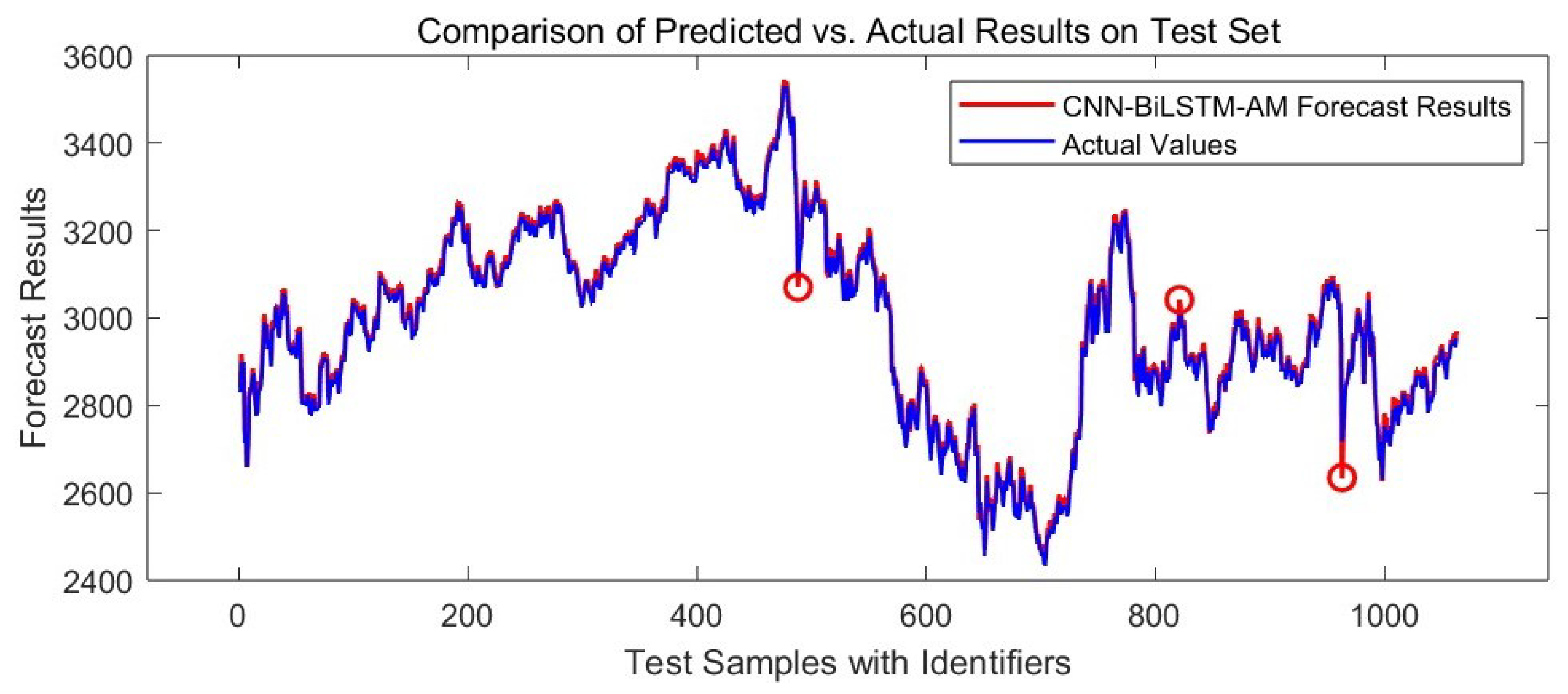
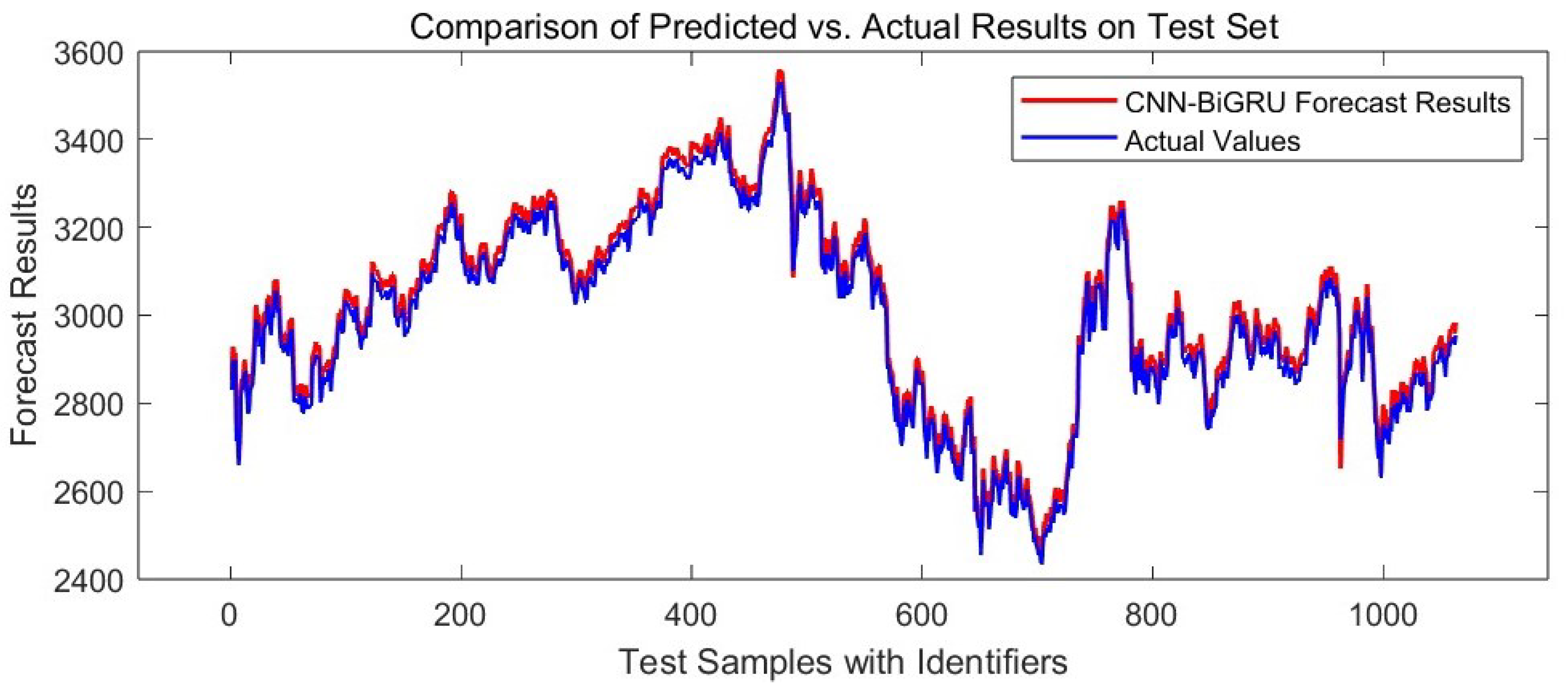
3.6.1. Line Chart Analysis

In order to demonstrate the effectiveness of the present method, we conducted an experimental comparison with several other models, including GRU, LSTM, GRU-AM, CNN-BiGRU, and CNN-BiLSTM, all of which were trained on the same dataset and evaluated using the same metrics. We then proceeded to analyze the results of this comparison, focusing on the two models with the best prediction performance among the set of compared models. To provide further visualization and analysis of the prediction effect comparison between the models, the test set was used to evaluate the CNN-BiLSTM-AM and LSTM models, as well as the CNN-BiGRU-AM model presented in this paper. The results are illustrated in Figure 9, Figure 10 and Figure 11.
Figure 9 illustrates that the model presented in this paper is capable of accurately capturing the trends and changes in the dataset, while also demonstrating a robust ability to capture local fluctuations. The high degree of overlap between the prediction curves and the actual values indicates that the model has a high degree of accuracy in predicting the actual data. This verifies the strong prediction ability and excellent generalization ability of the model, which is attributed to the model’s ability to be used at the CNN layer, the BiGRU layer, and the AM layer to learn and process the data at three levels, integrating local features, time dependence, and importance weights, while combining the data anomaly handling mechanism, which improves the flexibility and adaptability of stock data processing.
Upon further examination of Figure 10, it becomes evident that the overall fitting effect is also superior. However, it is notable that the three points marked by circles in the figure exhibit a considerable discrepancy between the comparison model and the actual data, particularly in the three above-mentioned instances. The data exhibit considerable volatility both before and after the above-mentioned points, which coincide with the most acute phase of the model’s operation. Distinguishing between anomalous and non-anomalous data at this juncture is challenging, resulting in a larger prediction error. This underscores the critical role of anomalous data processing in the overall model performance. This also underscores the significance of anomalous data processing.
Finally, an examination of Figure 11 reveals that the model exhibits a notable deficiency in curve overlap. This is primarily attributable to the absence of an AM layer, which impairs the model’s capacity to dynamically focus on the most salient aspects of the input data, thereby leading to an uneven distribution of information weights. Upon closer examination, it becomes evident that the model exhibits a similar issue of significant prediction error at the same three points as the CNN-BiLSTM-AM model. Additionally, it demonstrates an inability to effectively handle sudden changes, which can be attributed to the absence of incorporation of a data anomaly handling mechanism.

3.6.2. Analysis of Evaluation Indices

For further investigation, Table 2 lists the performance indices of this paper’s model and the comparison models on the test set.
As illustrated by the findings presented in the table, the CNN-BiGRU-AM model demonstrates the highest level of efficacy among the array of models examined, particularly in its capacity to predict stock prices with precision and to generate risk-adjusted returns. The subsequent analysis will delve into this aspect in greater detail.
First, in terms of prediction accuracy, the CNN-BiGRU-AM model has an RMSE of 22.027 and an MAE of 19.043, both of which are the smallest among all the models. This indicates that the CNN-BiGRU-AM model has the smallest prediction error, which means that it is able to predict stock prices more accurately and reduce the bias in the prediction. In comparison, the other models have larger RMSE and MAE. For example, CNN-BiLSTM-AM has an RMSE of 21.357 and an MAE of 20.252, which is slightly lower than CNN-BiGRU-AM, but still falls short of the best performance. The RMSE of CNN-BiGRU is 23.727 and the MAE is 21.851, and although its performance is also good, it is still higher than the previous two, which shows that its prediction accuracy is worse, which also indirectly suggests that the CNN-BiGRU-AM model outperforms the CNN-BiGRU model, which does not incorporate AM. The RMSE and MAE of BiGRU, LSTM, GRU-AM, and GRU models vary between 29. 671 and 24.231, 29.331 and 24.361, 27.391 and 24.991, 33.642 and 26.081, which are all significantly higher than CNN-BiGRU-AM and CNN-BiLSTM-AM, indicating that these models are less accurate in predicting stock market prices.
Second, in terms of the model’s ability to fit, the R 2 is an important measure of the model’s goodness of fit, as the closer the value is to 1, the better the model can explain the data. CNN-BiGRU-AM’s R 2 of 0.9903 is the highest among all the models, indicating that the model is able to fit the data very well, explaining most of the stock market’s price changes. In contrast, the R 2 of CNN-BiLSTM-AM is 0.9895, which is also a good performance but slightly inferior. The R 2 of CNN-BiGRU is 0.9801, which is still better than the other conventional models but still lower than CNN-BiGRU-AM and CNN-BiLSTM-AM. The R 2 of BiGRU, LSTM, GRU-AM, and GRU have R 2 values of 0.9725, 0.9770, 0.9712, and 0.9699, respectively, which are significantly lower than those of the former, indicating that these models are weak in fitting stock market price data, and fail to effectively capture the patterns of stock market price changes.
In terms of risk-adjusted returns, the Sharpe ratio is a key measure of the balance between risk and return. A higher Sharpe ratio indicates a higher return per unit of risk, which is an important reference for investors when choosing a model. As can be seen from the table, CNN-BiGRU-AM has a Sharpe ratio of 0.65, which is the highest among all the models, indicating that the model is able to better control the risk while providing a higher return, thus providing investors with a better risk-return ratio. In comparison, CNN-BiLSTM-AM has a slightly lower Sharpe ratio of 0.63, while CNN-BiGRU has a Sharpe ratio of 0.66, which is slightly higher than that of CNN-BiGRU-AM, but not significantly different. The Sharpe ratios of BiGRU are 0.56, LSTM 0.45, GRU-AM 0.53, CNN 0.48, and GRU at 0.51. The generally low Sharpe ratios of these models imply that their returns are accompanied by higher risks, and investors may face higher investment risks when using these models.

3.7. Discussion

A comparative analysis of the performance metrics reveals that the CNN-BiGRU-AM model demonstrates superior performance across all metrics, particularly in terms of accuracy and risk-adjusted returns. Specifically, the CNN-BiGRU-AM model exhibits the smallest values for RMSE and MAE, indicating minimal prediction error. Additionally, it attains the highest R 2 value, suggesting an optimal fit to the stock market data. Furthermore, the CNN-BiGRU-AM model demonstrates a Sharpe ratio of 0.65, suggesting that it performs notably well in terms of risk-adjusted returns and offers investors a higher potential for profitable investment returns.
A comparative analysis reveals that, while CNN-BiLSTM-AM exhibits a marginally lower RMSE and MAE, its R 2 and Sharpe ratio are not commensurate with those of CNN-BiGRU-AM. This observation suggests that CNN-BiGRU-AM may offer superior performance in stock market prediction. Although CNN-BiGRU exhibits a modest decline in accuracy relative to CNN-BiGRU-AM, its R 2 and Sharpe ratio demonstrate enhanced performance, maintaining competitiveness. In contrast, BiGRU, LSTM, GRU-AM, and GRU models demonstrate suboptimal performance, with their metrics displaying considerable lag, suggesting diminished capacity to capture stock market price fluctuations and inferior risk-return ratios.
To summarize the above-mentioned analysis, CNN-BiGRU-AM is unquestionably the most effective model in the study. This model demonstrates clear advantages in terms of accuracy, fitting ability, and risk-adjusted return. The incorporation of a BiGRU and an AM has been demonstrated to enhance the precision of stock market price prediction and optimize risk management, thereby ensuring higher returns. Consequently, CNN-BiGRU-AM emerges as the optimal model for stock price prediction, providing investors with a more reliable investment decision support system.

4. Conclusions

This study systematically addresses the two core challenges of nonlinear modeling and abnormal data interference in stock price prediction by constructing a CNN-BiGRU-AM hybrid model, achieving the following key advancements:
  • Multimodal Collaborative Optimization Mechanism: This mechanism enables the seamless integration of CNN-based local mutation feature extraction, BiGRU-based bidirectional time series modeling, and AM-AE-based dynamic feature purification, overcoming the limitations of traditional hybrid models that simply stack components. Experiments demonstrate that this architecture achieves an R 2 of 0.9903 for Shanghai Composite Index prediction, which is 0.08% higher than the best-performing baseline model, CNN-BiLSTM-AM ( R 2 = 0.9895), and 1% higher than the ablation comparison model, CNN-BiGRU ( R 2 = 0.9801), thereby validating the significant improvement in prediction accuracy through feature collaborative optimization.
  • Anomaly Immunity Prediction Paradigm: A three-stage anomaly handling framework, comprising “pre-detection, mid-filtering, and post-correction”, is proposed to overcome the limitations of isolated anomaly analysis in traditional approaches. By deeply integrating anomaly detection into the feature learning process, this paradigm enables adaptive feature optimization, mitigating the impact of anomalies while preserving the model’s ability to capture normal price mechanisms. This approach fosters an endogenous synergy between anomaly immunity and prediction optimization.
  • Risk-Return Balance Ability: Risk exposure is dynamically adjusted through the attention mechanism, resulting in a model Sharpe ratio of 0.65, which is 22.6% higher than that of GRU-AM (0.53) and 16.1% higher than BiGRU (0.56).
These findings not only offer a novel methodological framework for forecasting complex financial time series, but also uncover several practical principles:
  • Market Dynamics Analysis: The model feature weights reveal the underlying driving mechanisms of price fluctuations and offer a quantitative reference for understanding the multi-scale coupling effects within the market, such as the nonlinear interactions between macro policies and micro trading behaviors.
  • Investment Decision Optimization: The risk-return dynamic balance mechanism offers an adaptive regulatory framework for portfolio management, facilitating the transition from traditional experience-based strategies to a data-driven, intelligence-enhanced paradigm.
Future research can be deepened from three aspects:
  • Fusion of Multi-Source Heterogeneous Data: Incorporating unstructured information, such as news sentiment analysis (BERT), institutional holdings data (13F Filings), and public opinion factors, to construct a cross-modal prediction system is anticipated to enhance prediction accuracy.
  • Real-Time Decision Support: Explore lightweight deployment solutions to address the low-latency prediction requirements in high-frequency trading scenarios.
  • Enhanced Interpretability: SHAP values are employed to analyze the model’s decision logic, with a focus on uncovering the impact of nonlinear feature interactions on prediction outcomes.

Author Contributions

J.L. proposed the project model and wrote the manuscript. Y.C. helped to improve the model and conduct the experiments. K.X. provided the original data and gave useful suggestions during the research process. C.W. played a key role in the formal analysis. Y.R. played a key role in conducting the survey. J.J. made great contributions in project supervision and investigation. J.H. was responsible for funding acquisition and obtaining the funds. W.Z. provided valuable support in validation and played a key role in obtaining the funds. All authors have read and agreed to the published version of the manuscript.

Funding

This research was funded by the National Natural Science Foundation of China (Grant No. 62373372) and the National Natural Science Foundation of China (Grant No. 62272485). Furthermore, we acknowledge that the main research activities described in this paper were conducted as part of the Innovative Entrepreneurship Undergraduate Training Programme [Grant No. Yz2024410] at Yangtze University.

Institutional Review Board Statement

Not applicable.

Informed Consent Statement

Informed consent was obtained from all subjects involved in the study.

Data Availability Statement

The dataset presented in this paper is obtained from the stock data of the Shanghai Composite Index, which was sourced from the Tushare platform. The data have been authorized for use by the Platform. As required, the data are not publicly available. However, researchers interested in accessing the data may contact Jiacheng Luo at 2022005435@yangtzeu.edu.cn to discuss potential collaborations or data-sharing agreements.

Conflicts of Interest

The authors declare that they have no known competing financial interests or personal relationships that could have appeared to influence the work reported in this paper.

Abbreviations

The following abbreviations are used in this manuscript:
CNNsConvolutional Neural Networks
BiGRUBidirectional Gated Recurrent Unit
AMAttention Mechanism
GRUGated Recurrent Unit
RNNsRecurrent Neural Networks
LSTMLong Short-Term Memory Network
13FilingsSEC Form 13F

References

  1. Badea, L.; Ionescu, V.; Guzun, A.A. What is the causal relationship between stoxx europe 600 sectors? but between large firms and small firms? Econ. Comput. Econ. Cybern. Stud. Res. 2019, 53, 5–20. [Google Scholar] [CrossRef]
  2. Mandal, R.C.; Kler, R.; Tiwari, A.; Keshta, I.; Abonazel, M.R.; Tageldin, E.M.; Umaralievich, M.S. Enhancing Stock Price Prediction with Deep Cross-Modal Information Fusion Network. Fluct. Noise Lett. 2024, 23, 2440017. [Google Scholar] [CrossRef]
  3. Wahlen, J.M.; Wieland, M.M. Can financial statement analysis beat consensus analysts’ recommendations? Rev. Account. Stud. 2011, 16, 89–115. [Google Scholar] [CrossRef]
  4. Barberis, N.; Mukherjee, A.; Wang, B. Prospect Theory and Stock Returns: An Empirical Test. Rev. Financ. Stud. 2016, 29, 3068–3107. [Google Scholar] [CrossRef]
  5. Temur, G.; Birogul, S.; Kose, U. Comparison of Stock “Trading” Decision Support Systems Based on Object Recognition Algorithms on Candlestick Charts. IEEE Access 2024, 12, 83551–83562. [Google Scholar] [CrossRef]
  6. Beniwal, M.; Singh, A.; Kumar, N. A comparative study of static and iterative models of ARIMA and SVR to predict stock indices prices in developed and emerging economies. Int. J. Appl. Manag. Sci. 2023, 15, 352–371. [Google Scholar] [CrossRef]
  7. Jarrah, M.; Derbali, M. Predicting Saudi Stock Market Index by Using Multivariate Time Series Based on Deep Learning. Appl. Sci. 2023, 13, 8356. [Google Scholar] [CrossRef]
  8. Houssein, E.H.; Dirar, M.; Abualigah, L.; Mohamed, W.M. An efficient equilibrium optimizer with support vector regression for stock market prediction. Neural Comput. Appl. 2022, 34, 3165–3200. [Google Scholar]
  9. Akhtar, M.M.; Zamani, A.S.; Khan, S.; Shatat, A.S.A.; Dilshad, S.; Samdani, F. Stock market prediction based on statistical data using machine learning algorithms. J. King Saud Univ.-Sci. 2022, 34, 101940. [Google Scholar]
  10. Zakhidov, G. Economic indicators: Tools for analyzing market trends and predicting future performance. Int. Multidiscip. J. Univ. Sci. Prospect. 2024, 2, 23–29. [Google Scholar]
  11. Billah, M.M.; Sultana, A.; Bhuiyan, F.; Kaosar, M.G. Stock price prediction: Comparison of different moving average techniques using deep learning model. Neural Comput. Appl. 2024, 36, 5861–5871. [Google Scholar] [CrossRef]
  12. Kaya, D.; Reichmann, D.; Reichmann, M. Out-of-sample predictability of firm-specific stock price crashes: A machine learning approach. J. Bus. Financ. Account. 2024. early view. [Google Scholar] [CrossRef]
  13. Xu, X.; Ye, T.; Gao, J.; Chu, D. The effect of green, supply chain factors in predicting China’s stock price crash risk: Evidence from random forest model. Environ. Dev. Sustain. 2024. [Google Scholar] [CrossRef]
  14. Sulastri, H.; Intani, S.M.; Rianto, R. Application of bagging and particle swarm optimisation techniques to predict technology sector stock prices in the era of the COVID-19 pandemic using the support vector regression method. Int. J. Comput. Sci. Eng. 2023, 26, 255–267. [Google Scholar] [CrossRef]
  15. Liu, J.X.; Leu, J.S.; Holst, S. Stock price movement prediction based on Stocktwits investor sentiment using FinBERT and ensemble SVM. PeerJ Comput. Sci. 2023, 9, e1403. [Google Scholar] [CrossRef] [PubMed]
  16. Vuong, P.H.; Phu, L.H.; Nguyen, T.H.V.; Duy, L.N.; Bao, P.T.; Trinh, T.D. A bibliometric literature review of stock price forecasting: From statistical model to deep learning approach. Sci. Prog. 2024, 107, 00368504241236557. [Google Scholar] [CrossRef]
  17. Chang, V.; Xu, Q.A.; Chidozie, A.; Wang, H. Predicting Economic Trends and Stock Market Prices with Deep Learning and Advanced Machine Learning Techniques. Electronics 2024, 13, 3396. [Google Scholar] [CrossRef]
  18. Carosia, A.E.d.O.; da Silva, A.E.A.; Coelho, G.P. Predicting the Brazilian Stock Market with Sentiment Analysis, Technical Indicators and Stock Prices: A Deep Learning Approach. Comput. Econ. 2024. [Google Scholar] [CrossRef]
  19. Das, N.; Sadhukhan, B.; Bhakta, S.S.; Chakrabarti, S. Integrating EEMD and ensemble CNN with X (Twitter) sentiment for enhanced stock price predictions. Soc. Netw. Anal. Min. 2024, 14, 29. [Google Scholar] [CrossRef]
  20. Rath, S.; Das, N.R.; Pattanayak, B.K. Stacked BI-LSTM and E-Optimized CNN-A Hybrid Deep Learning Model for Stock Price Prediction. Opt. Memory Neural Netw. 2024, 33, 102–120. [Google Scholar] [CrossRef]
  21. Tian, B.; Yan, T.; Yin, H. Forecasting the Volatility of CSI 300 Index with a Hybrid Model of LSTM and Multiple GARCH Models. Comput. Econ. 2024. [Google Scholar] [CrossRef]
  22. Tu, S.; Huang, J.; Mu, H.; Lu, J.; Li, Y. Combining Autoregressive Integrated Moving Average Model and Gaussian Process Regression to Improve Stock Price Forecast. Mathematics 2024, 12, 1187. [Google Scholar] [CrossRef]
  23. Huo, Y.; Jin, M.; You, S. A study of hybrid deep learning model for stock asset management. PeerJ Comput. Sci. 2024, 10, e2493. [Google Scholar] [CrossRef] [PubMed]
  24. Ma, W.; Hong, Y.; Song, Y. On Stock Volatility Forecasting under Mixed-Frequency Data Based on Hybrid RR-MIDAS and CNN-LSTM Models. Mathematics 2024, 12, 1538. [Google Scholar] [CrossRef]
  25. Mu, S.; Liu, B.; Gu, J.; Lien, C.; Nadia, N. Research on Stock Index Prediction Based on the Spatiotemporal Attention BiLSTM Model. Mathematics 2024, 12, 2812. [Google Scholar] [CrossRef]
  26. Duan, G.; Yan, S.; Zhang, M. A Hybrid Neural Network Model for Sentiment Analysis of Financial Texts Using Topic Extraction, Pre-Trained Model, and Enhanced Attention Mechanism Methods. IEEE Access 2024, 12, 98207–98224. [Google Scholar] [CrossRef]
  27. Jayanth, T.; Manimaran, A.; Siva, G. Enhancing Stock Price Forecasting With a Hybrid SES-DA-BiLSTM-BO Model: Superior Accuracy in High-Frequency Financial Data Analysis. IEEE Access 2024, 12, 173618–173637. [Google Scholar] [CrossRef]
  28. Thi, H.L.; Nguyen, T. Variational Quantum Algorithms in Anomaly Detection, Fraud Indicator Identification, Credit Scoring, and Stock Price Prediction. In Proceedings of Ninth International Congress on Information and Communication Technology, ICICT 2024; Yang, X., Sherratt, S., Dey, N., Joshi, A., Eds.; Lecture Notes in Networks and Systems; Springer: Singapore, 2024; Volume 1003, pp. 483–492. [Google Scholar] [CrossRef]
  29. Wu, K.; Karmakar, S.; Gupta, R.; Pierdzioch, C. Climate Risks and Stock Market Volatility over a Century in an Emerging Market Economy: The Case of South Africa. Climate 2024, 12, 68. [Google Scholar] [CrossRef]
  30. Liu, H.; Dahal, B.; Lai, R.; Liao, W. Generalization error guaranteed auto-encoder-based nonlinear model reduction for operator learning. Appl. Comput. Harmon. Anal. 2025, 74, 101717. [Google Scholar] [CrossRef]
  31. Biswas, D.; Gil, J.M. Design and Implementation for Research Paper Classification Based on CNN and RNN Models. J. Internet Technol. 2024, 25, 637–645. [Google Scholar] [CrossRef]
  32. Weerasena, H.; Mishra, P. Revealing CNN Architectures via Side-Channel Analysis in Dataflow-based Inference Accelerators. ACM Trans. Embed. Comput. Syst. 2024, 23, 1–25. [Google Scholar] [CrossRef]
  33. Tharun, S.B.; Jagatheswari, S. A U-shaped CNN with type-2 fuzzy pooling layer and dynamical feature extraction for colorectal polyp applications. Eur. Phys. J.-Spec. Top. 2024. [Google Scholar] [CrossRef]
  34. Luo, H.; Chen, J.; Sun, Z.; Zhang, Y.; Zhang, L. Improved Marine Predators Algorithm Optimized BiGRU for Strip Exit Thickness Prediction. IEEE Access 2024, 12, 56719–56729. [Google Scholar] [CrossRef]
  35. Li, D.; Li, W.; Zhao, Y.; Liu, X. The Analysis of Deep Learning Recurrent Neural Network in English Grading Under the Internet of Things. IEEE Access 2024, 12, 44640–44647. [Google Scholar] [CrossRef]
  36. Sun, W.; Chen, J.; Hu, C.; Lin, Y.; Wang, M.; Zhao, H.; Zhao, R.; Fu, G.; Zhao, T. Clock bias prediction of navigation satellite based on BWO-CNN-BiGRU-attention model. GPS Solut. 2025, 29, 46. [Google Scholar] [CrossRef]
  37. Fan, J.; Yang, H.; Li, X.; Jiang, Y.; Wu, Z. Prediction of FeO content in sintered ore based on ICEEMDAN and CNN-BiLSTM-AM. Ironmak. Steelmak. 2025. [Google Scholar] [CrossRef]
Figure 1. General algorithm flowchart.
Electronics 14 01275 g001
Figure 2. Diagram of auto-encoder’s structure.
Electronics 14 01275 g002
Figure 3. Illustration of the structure of CNN.
Electronics 14 01275 g003
Figure 4. Structure of BiGRU.
Electronics 14 01275 g004
Figure 5. Structure of GRU.
Electronics 14 01275 g005
Figure 6. Illustration of the principle of the attention mechanism.
Electronics 14 01275 g006
Figure 7. Auto-encoder anomaly detection reconstruction error comparison.
Electronics 14 01275 g007
Figure 8. Regression analysis of CNN-BiGRU-AM on test set.
Electronics 14 01275 g008
Figure 9. Performance of CNN-BiGRU-AM.
Electronics 14 01275 g009
Figure 10. Performance of CNN-BiLSTM-AM.
Electronics 14 01275 g010
Figure 11. Performance of CNN-BiGRU.
Electronics 14 01275 g011
Table 1. Model hyper-parameters and details.
HyperparameterApplicable ScopeValueRemarks
MaxEpochsCNN-BiGRU-AM200Maximum number of training epochs for the entire model.
Initial Learning RateCNN-BiGRU-AM0.001The initial learning rate of the entire model.
BatchSizeCNN-BiGRU-AM64The batch size during each training iteration.
L2 Regularization FactorCNN-BiGRU-AM1 × 10−5The parameter that prevents overfitting.
Learning Rate Decay FactorCNN-BiGRU-AM0.5Factor for controlling the decay of the learning rate.
Learning Rate Decay PeriodCNN-BiGRU-AM150Period for controlling learning rate decay.
Number of Filters in Convolutional LayerCNN Layer16/3216 is the number of filters in the first convolutional layer, and 32 in the second.
Kernel SizeCNN Layer[1, 1]The size of the convolutional kernels in the convolutional layer is 1 × 1.
Activation FunctionCNN LayerReLUThe activation function
GRU UnitsBiGRU Layer50Number of units in a single GRU layer to process the sequential data.
Activation FunctionBiGRU LayerReLUThe activation function
Number of Neurons in Fully Connected LayerAM Layer8/32The first layer(8) compresses features, and the second(32) generates more detailed features for attention weight calculation.
Activation FunctionAM LayerSigmoidThis function is used to generate attention weights.
Activation FunctionAM LayerReLUThe activation function
Table 2. Performance metrics for each model on the test set.
ModelRMSEMAER2Sharpe Ratio
CNN-BiGRU-AM22.02719.0430.99030.65
CNN-BiLSTM-AM21.35720.2520.98950.63
CNN-BiGRU23.72721.8510.98010.66
BiGRU29.67124.2310.97250.56
LSTM29.33124.3610.97700.45
GRU-AM27.39124.9910.97120.53
CNN30.25425.6210.96820.48
GRU33.64226.0810.96990.51
Disclaimer/Publisher’s Note: The statements, opinions and data contained in all publications are solely those of the individual author(s) and contributor(s) and not of MDPI and/or the editor(s). MDPI and/or the editor(s) disclaim responsibility for any injury to people or property resulting from any ideas, methods, instructions or products referred to in the content.

