Terrain-Aware Hierarchical Control Framework for Dynamic Locomotion of Humanoid Robots

Abstract

Dynamic locomotion capabilities on complex terrains constitute a critical requirement for humanoid robots in industrial manufacturing and emergency response applications. To address the fundamental challenges of terrain perception, underactuated dynamics planning, and foothold control in unstructured environments, this paper proposes a hierarchical planning and control framework that integrates terrain perception. The framework first segments the terrain to generate convex polygon constraints that characterize the terrain features. Subsequently, an optimization model is constructed based on nonlinear model predictive control, integrating underactuated dynamics and terrain constraints into a multi-objective optimal control problem. This problem is solved in real time using sequential quadratic programming. Furthermore, a hierarchical whole-body control approach is employed, which achieves coordinated whole-body control under multiple tasks and constraints through priority task allocation and quadratic programming. We validate the proposed methods through simulated experiments on forward walking, external force disturbance, and complex terrain walking conducted on the MuJoCo simulation platform. The simulation demonstrates that the robot can achieve a stable walking speed of 1 m/s and possess forward and lateral anti-disturbance capabilities of 60 Ns and 30 Ns, respectively. The robot can also stably traverse stairs with a height difference of 0.16 m and random terrains. These results validate the advantages of the proposed method in terms of dynamic performance, robustness, and terrain adaptability.

1. Introduction

The ultimate objective of legged robots is to achieve autonomous locomotion and operation in complex, unstructured, and unknown environments, which imposes stringent requirements on the robot’s perception, planning, and control algorithms [1,2,3,4]. Humanoid robots, with their human-like structure and motion patterns, offer distinct advantages in mitigating risks such as jolting, slipping, and immobilization in unstructured environments by adaptive foothold selection, gait adjustment, and speed modulation. Their strong locomotion capabilities in complex environments enable a wide range of applications such as disaster response, industrial automation, and space exploration. However, the motion planning and control of humanoid robots are inherently complex due to their high degrees of freedom, and the reliance on precise terrain perception in such environments further adds to the challenges in their research and practical deployment.

Current model-based methodologies for humanoid locomotion have predominantly focused on two aspects: (a) perceptive locomotion utilizing static gaits [5,6,7,8,9] and (b) blind dynamic locomotion under the assumption of flat terrain [10,11,12]. While recent advances in learning-based control frameworks have demonstrated remarkable generalization capabilities, enabling robust locomotion across diverse challenging terrains without explicit terrain models [13,14,15,16,17,18], research on vision-guided reinforcement learning for humanoid robots remains limited [19,20]. Despite these advancements, the integration of terrain perception modules for precise foothold control on rugged terrains remains a significant challenge. This integration challenge manifests through three bottlenecks: computationally efficient terrain representation, optimal foothold selection in unstructured environments, and coordinated planning of underactuated system dynamics.

In the context of foothold selection, several studies have incorporated perceptual information into foothold selection algorithms [21,22,23], adopting a hierarchical framework where foothold positions and base motion are optimized independently. In this framework, the high-level module selects footholds by incorporating terrain information, while the low-level module optimizes base motion based on the robot’s dynamic model. Although this hierarchical approach reduces computational complexity, it requires manual alignment between these two modules. Furthermore, the independent optimization of footholds and base motion often fails to adequately address kinematic constraints between the base and legs, as well as leg collision avoidance with the terrain.

In contrast, some studies have proposed a joint optimization approach for foothold positions and base motion, simultaneously considering both base and leg movements during trajectory optimization, which has yielded promising results [24,25,26]. This method eliminates the need for manual handling of the coupled motion between the legs and base and allows for the integration of comprehensive terrain information into the optimization process. However, the joint optimization of base and leg motion introduces significant computational complexity due to the high-dimensional nature of the model, particularly when perceptual information is incorporated. This may result in excessively long computation times, making it challenging to achieve real-time deployment.

Elevation maps play a crucial role in terrain perception and are extensively utilized in the navigation and control of legged robots [27,28,29]. Algorithms based on search or sampling techniques can identify stable foothold positions by leveraging ground height information derived from elevation maps. In optimization-based control algorithms, elevation maps are commonly employed as inputs and integrated with other constraints to optimize the robot’s motion or path planning. For instance, Winkler et al. [25] employed elevation maps for foothold selection and collision avoidance, applying equality constraints to restrict the start and endpoints of foot trajectories to the terrain and inequality constraints to prevent collisions between the swing foot and the terrain. However, this approach does not account for the discontinuities and non-convexities of the terrain, which may cause the optimization problem to converge to local minima, thereby limiting its effectiveness in complex environments.

In the domain of trajectory optimization, large-scale nonlinear solvers such as SNOPT [30] and IPOPT [31] are widely adopted [32,33]. These solvers are capable of handling the complex constraints and objective functions inherent to nonlinear optimization problems, although they often require extensive iterative computations to find optimal solutions. Alternatively, specialized solvers for trajectory optimization, such as iterative Linear Quadratic Regulator (iLQR) [34,35] and Sequential Linear Quadratic (SLQ) methods [36], have been proposed. These solvers, which are variants of Differential Dynamic Programming (DDP) [37], can efficiently compute near-optimal solutions within a relatively short time frame, making them particularly suitable for high-dimensional problems. Nevertheless, these methods still require linearization of the system, which may introduce approximation errors during the computation process and potentially compromise the accuracy of the solutions.

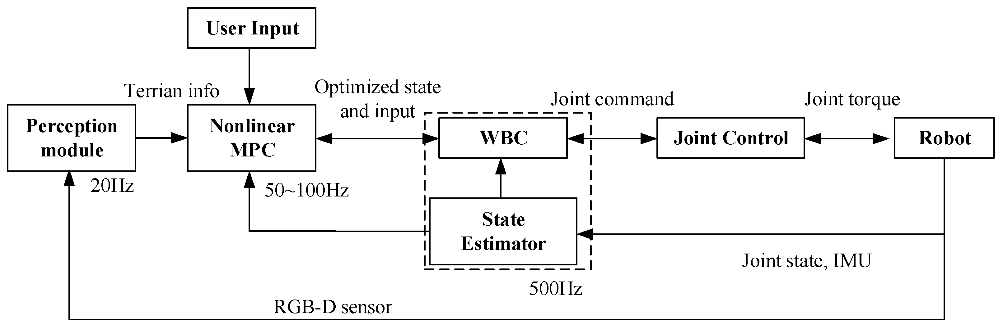
To address the aforementioned challenges, this paper proposes a hierarchical planning and control framework that integrates terrain perception. As illustrated in Figure 1, the framework comprises a three-level architecture: perception, planning, and control. The perception layer constructs a high-precision elevation map from 3D point cloud data, extracts feasible regions through terrain segmentation, and generates convex polygon terrain constraints. The motion planning layer formulates a multi-objective optimization problem that incorporates underactuated dynamics constraints and terrain constraints using nonlinear model predictive control (MPC). A sequential quadratic programming (SQP) algorithm is employed to generate gaits and trajectories in real time within 10 ms to 20 ms. The whole-body control (WBC) layer adopts a hierarchical optimization strategy, utilizing null-space projection and quadratic programming to coordinate multiple tasks and constraints, thereby achieving synergistic optimization of dynamic balance and trajectory tracking. The three-layer architecture operates as an integrated system through closed-loop feedback mechanisms. The key contributions of this paper are as follows:

• Real-time trajectory planning via nonlinear MPC: we implemented trajectory planning for humanoid robots using nonlinear MPC, with real-time gait and trajectory generation achieved via an SQP algorithm.
• Closed-loop architecture with triple coupling: we constructed a closed-loop architecture featuring “perception–planning–control” triple coupling, enabling the deep integration of terrain perception with underactuated system planning and control.
• High-performance locomotion capabilities: Based on the proposed method, the simulated experiments demonstrate high-performance capabilities on humanoid robots, including high-speed walking at 1 m/s, disturbance rejection with up to 60 Ns in the forward direction and 30 Ns in the lateral direction, and obstacle traversal over heights of 0.16 m, representing a significant improvement in locomotion performance on complex terrains.

Following the proposed framework, the structure of this paper is organized as follows: Section 2 presents the details on the terrain perception pipeline. Subsequently, the formulation of the motion planning problem and the corresponding numerical optimization strategy are presented in Section 3 and Section 4, respectively. Section 5 introduces the whole-body control layer. Finally, the proposed method is evaluated on the MuJoCo simulation platform in Section 6, and the paper concludes with a summary in Section 7.

2. Terrain Perception

To establish a geometric model of terrain in complex environments, this section utilizes point cloud data acquired from RGB-D sensors to construct a 2.5D elevation map that incorporates sensor uncertainty and robot pose uncertainty. The elevation map is further segmented to extract critical terrain features.

2.1. Elevation Map Construction

Constructing a robot-centric local elevation map requires projecting depth images from the sensor onto a cell grid map. Unlike global maps defined in an inertial coordinate system, the local map is continuously updated with robot motion without relying on absolute localization. To account for uncertainties in depth measurements and locomotion-induced pose variations on unstructured terrains, we employ the elevation map update algorithm proposed in [38].

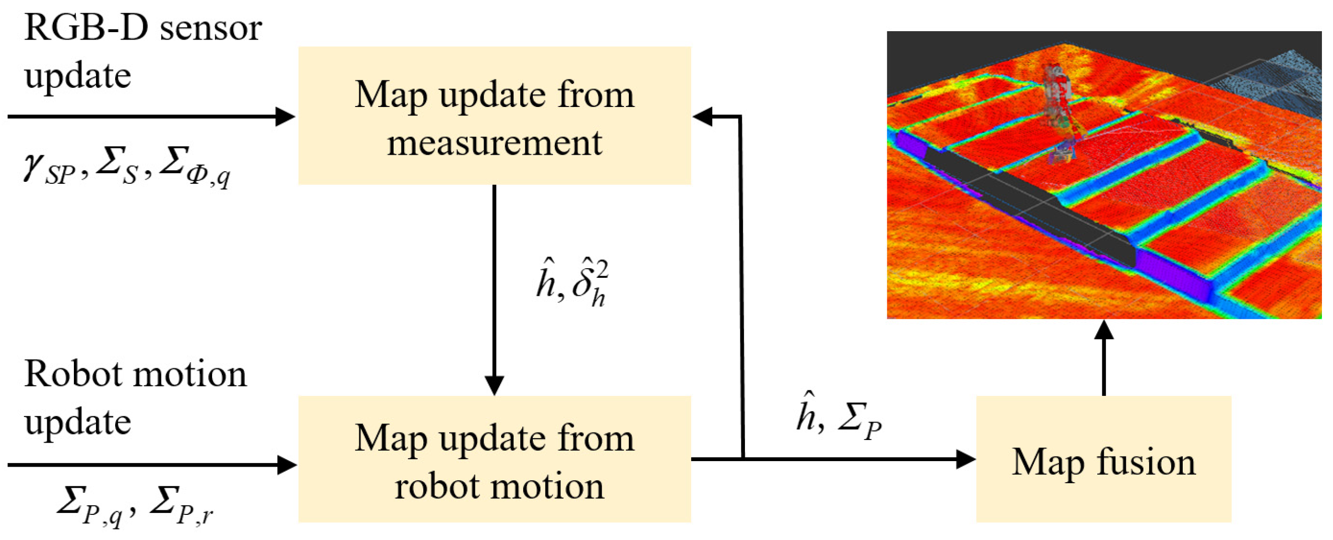
The update process of the elevation map is illustrated in Figure 2. Initially, based on the depth distance vector, ${\mathit{\gamma }}_{SP}$, of point P on the terrain measured by the sensor, the covariance matrix, ${\mathit{\Sigma }}_S$, of the sensor model, and the covariance matrix, ${\mathit{\Sigma }}_{\Phi ,q}$, of the sensor’s rotation relative to the map coordinate system, a one-dimensional Kalman filter is applied to fuse the old and new elevation measurements to update the mean, $\widehat{h}$, and variance values, ${\widehat{\delta }}_h^2$, of the elevation map.

Given that the elevation map moves with the robot, the spatial covariance matrix, ${\mathit{\Sigma }}_P$, of each cell in the elevation map is updated whenever the robot’s pose changes, based on the robot’s translational covariance, ${\mathit{\Sigma }}_{P,r}$, and rotational covariance matrix, ${\mathit{\Sigma }}_{P,q}$. Finally, the height estimate for each cell is computed as a weighted mean of the heights from surrounding cells in a process known as map fusion.

2.2. Plane Segmentation

The objective of terrain segmentation is to identify traversable regions and boundaries based on terrain parameters. Slope and roughness, which serve as critical indicators for characterizing terrain, reflect the inclination and irregularity of the terrain, respectively. Feasibility classification is performed using the local surface inclination and the local roughness, the latter of which is estimated through the standard deviation [39]. For a neighborhood of size N, these quantities are computed as follows:

$$\mathit{\mu }={\displaystyle \frac{1}{N}}{\displaystyle \mathbf{\sum }_i{r}_i}$$

(1)

$$\mathit{S}={\displaystyle \frac{1}{N}}{\displaystyle \sum _i{r}_i{r}_i^T}$$

(2)

$$\mathit{\Sigma }=\mathit{S}-\mathit{\mu }{\mathit{\mu }}^T$$

(3)

where μ and S denote the mean and variance of the cell height r_i, respectively, while Σ represents the positive semi-definite covariance matrix of r_i.

The variance of the local surface normal direction ${\sigma }_h^2$ corresponds to the smallest eigenvalue of Σ, and the surface normal vector n is the eigenvector associated with this smallest eigenvalue. In this study, a neighborhood of N = 16 is used, with the standard deviation threshold for the normal direction set to 2 cm and the maximum slope angle set to 20°. If the angle is below the threshold and the standard deviation is less than the threshold, the region is classified as planar. A cell is marked with 1 if its neighborhood satisfies the planar condition; otherwise, it is marked with 0. Finally, an opening operation is applied to the image to remove isolated points.

Upon completion of the feasibility classification, the connected component-labeling algorithm is employed to identify continuous regions. For each connected region, planarity verification is performed using the same method as in the previous classification. Subsequently, the determination of whether the region constitutes a plane is made based on the following criteria:

$$is plane=\left\{\begin{array}{cc}1\hfill & \hfill \mathit{if} {\sigma }_n\le 0.025,n_z\ge 0.96\\ 0\hfill & \hfill \mathit{otherwise}\end{array}\right.$$

(4)

To define a plane more accurately, the threshold for standard deviation is relaxed to 2.5 cm, allowing for a certain degree of topographic undulation. Meanwhile, the constraint on slope is tightened to 15°, ensuring that only planes meeting this stricter slope requirement are accepted. The final connected regions are subjected to erosion operations. By extracting the edges, the non-convex two-dimensional contours of each plane are obtained and projected onto the corresponding planes along the z-axis to define the boundaries within the planes.

3. Motion Planning

The motion planning of legged robots in complex terrains requires simultaneous consideration of dynamic constraints and physical constraints. By dynamically adjusting footholds and body posture, stability can be maintained across varying terrain conditions. This section describes how the motion planning problem for humanoid robots is transformed into an optimal control problem, incorporating terrain information, dynamic models, and other physical constraints into the modeling and solution processes.

3.1. Robot Definition

The schematic diagram of the humanoid robot’s structure is illustrated in Figure 3. Each leg is configured with six degrees of freedom, and each arm is configured with four degrees of freedom. An inertial coordinate system I is defined, with its x-axis aligned with the robot’s forward direction, the z-axis oriented vertically upward, and the y-axis determined according to the right-hand rule. The floating base coordinate system B is attached to the robot’s body, with its origin located at a specific point on the body. The initial orientation of B is aligned with that of the inertial coordinate system I. The center-of-mass coordinate system G is defined such that its origin coincides with the robot’s center of mass, and its orientation remains consistent with that of the inertial coordinate system I.

The generalized coordinates q and generalized velocities $\dot{q}$ of the robot are defined as follows:

$$\mathit{q}=\left[\begin{array}{c}{p}_B\\ {\theta }_B^{zyx}\\ q_j\end{array}\right]\in {ℝ}^{n_a+6}$$

(5)

$$\dot{q}=\left[\begin{array}{c}{\dot{p}}_B\\ {\dot{\theta }}_B\\ {\dot{q}}_j\end{array}\right]\in {ℝ}^{n_a+6}$$

(6)

where $p_B$ denotes the position of the floating base in the inertial coordinate system I, ${\theta }_B^{zyx}$ represents the orientation of the floating base in I, described by ZYX Euler angles, $q_j$ and ${\dot{q}}_j$ denote the joint angles and velocities of the actuated joints.

The contact between the humanoid robot’s foot and the environment is modeled as a surface contact, which is simplified to four contact points on the sole. Each contact point is subjected to a three-dimensional linear force ${\mathit{f}}_i$ from the environment. The set of forces acting on the robot’s foot contact points is denoted as $\mathit{f}\in {ℝ}^{24}$.

3.2. Dynamics Model

The state x and input u of the robot are defined as follows:

$$x={\left[\begin{array}{ccc}{h}_{\mathit{com}}& q_b& q_j\end{array}\right]}^T\in {ℝ}^{12+n_a}$$

(7)

$$u={\left[\begin{array}{cc}f& {\dot{q}}_j\end{array}\right]}^T\in {ℝ}^{3n_c+n_a}$$

(8)

where $h_{\mathit{com}}={\left[\begin{array}{cc}{h}_l& h_k\end{array}\right]}^T\in {ℝ}^6$ represents the robot’s centroidal momentum expressed in the center-of-mass coordinate system G, which comprises the linear momentum $h_l\in {ℝ}^3$ and the angular momentum $h_k\in {ℝ}^3$. $q_b={\left[\begin{array}{cc}{p}_B& {\theta }_B^{ZYX}\end{array}\right]}^T\in {ℝ}^6$ denotes the pose of the floating base in the inertial coordinate system I. n_a and n_c represent the number of actuated joints and contact points, respectively.

According to the centroidal dynamics, the external forces acting on the robot are equivalent to the rate of change in the centroidal momentum, which is expressed as follows:

$${\dot{h}}_{\mathit{com}}=\left[\begin{array}{c}{\displaystyle \sum _{i=1}^{n_c}{f}_i}+mg\\ {\displaystyle \sum _{i=1}^{n_c}{r}_{\mathit{com}2c_i}}\times f_i\end{array}\right]$$

(9)

where $r_{\mathit{com}2c_i}$ denotes the vector from the centroid to the i-th contact point, and f_i denotes the external force acting on the i-th contact point.

To solve for the centroidal momentum of the robot, a centroidal momentum matrix $A\left(q\right)\in {ℝ}^{6\times \left(6+n_a\right)}$ is introduced. This matrix describes the linear mapping between the generalized joint velocities $\dot{q}$ and the centroidal momentum h_com, expressed as follows:

$$h_{\mathit{com}}=A\left(q\right)\left[\begin{array}{c}{\dot{q}}_b\\ {\dot{q}}_j\end{array}\right]=\left[\begin{array}{cc}{A}_b\left(q\right)& A_j\left(q\right)\end{array}\right]\left[\begin{array}{c}{\dot{q}}_b\\ {\dot{q}}_j\end{array}\right]$$

(10)

Based on Equation (10), the velocity of the floating base ${\dot{\mathit{q}}}_b\in {ℝ}^6$ can be derived as follows:

$${\dot{\mathit{q}}}_b={\left({\mathit{A}}_b\left(\mathit{q}\right)\right)}^{-1}\left({\mathit{h}}_{\mathit{com}}-{\mathit{A}}_j\left(\mathit{q}\right){\dot{\mathit{q}}}_j\right)$$

(11)

By differentiating the robot state x, the state equation of the robot system is obtained as follows:

$$\dot{x}=\left[\begin{array}{c}\dot{h}\\ {\dot{q}}_b\\ {\dot{q}}_j\end{array}\right]=\left[\begin{array}{c}{\displaystyle \sum _{i=1}^{n_c}{f}_i+mg}\\ {\displaystyle \sum _{i=1}^{n_c}{r}_{com2c_i}\times f_i}\\ A_b^{-1}\left(h_{\mathit{com}}-A_j{\dot{q}}_j\right)\\ {\dot{q}}_j\end{array}\right]=\mathrm{f}\left(\mathit{x},\mathit{u}\right)$$

(12)

3.3. Trajectory Planning

3.3.1. Floating Base Trajectory Planning

The floating base position and orientation of a robot walking on complex terrain are intrinsically linked to terrain information and the user’s input commands. Assuming that the user’s input command velocities, comprising the linear velocities v_x and v_y in the horizontal plane and the angular velocity ω_yaw around the z-axis, remain constant. The horizontal position of the robot’s body in the inertial coordinate frame I can be derived as follows:

$$\left[\begin{array}{c}{x}_B^{ref}\\ y_B^{ref}\\ 0\end{array}\right]=\left[\begin{array}{c}{x}_B\\ y_B\\ 0\end{array}\right]+{}^{I}R_B\left[\begin{array}{c}{v}_x\Delta t\\ v_y\Delta t\\ 0\end{array}\right]$$

(13)

where x_B and y_B represent the current positions of the robot’s body in the inertial coordinate frame I, as computed by the state estimation module. The term ${}^{I}R_B$ denotes the rotation matrix between the body coordinate frame B and the inertial coordinate frame I. v_xΔt and v_yΔt represent the incremental position of the robot over the time window of Δt, expressed in the body coordinate frame B.

Similarly, the command for the rotation of the robot’s body around the z-axis can be expressed in the inertial coordinate frame I as follows:

$${\theta }_{\mathit{yaw},B}^{\mathit{ref}}={\theta }_{\mathit{yaw},B}+{\omega }_{\mathit{yaw}}\Delta t$$

(14)

During typical robot locomotion, the height command for the robot’s body is maintained at a constant value h_nom, which refers to the height of the floating base relative to the foot contact points. To determine the height of the floating base in the inertial coordinate frame I, a function z_map(x, y) is designed, and interpolation methods are employed to obtain the terrain height corresponding to a specified position (x, y).

3.3.2. Foothold Planning

Without considering the terrain, the nominal foothold is determined by integrating gait information with the floating base trajectory. Based on the heuristic foothold theory proposed by Raibert [40], the nominal foothold can be expressed as follows:

$$P_{i,\mathit{nom}}=P_{i,B,\mathit{nom}}+\sqrt{{\displaystyle \frac{h_{\mathit{nom}}}{g}}}\left(v_B-v_B^{\mathit{ref}}\right)$$

(15)

where $P_{i,\mathit{nom}}\in {ℝ}^3$ represents the nominal foothold in the inertial coordinate frame I; $P_{i,B,\mathit{nom}}\in {ℝ}^3$ denotes the position of the floating base at the midpoint of the support phase; g is the gravitational acceleration; and $v_B,v_B^{\mathit{ref}}\in {ℝ}^3$ represents the measured velocity and commanded velocity of the robot’s floating base, respectively. Equation (15) enables the closed-loop control of the robot’s velocity through foothold selection, which is critical for dynamic stability. For instance, if the measured velocity of the robot under external disturbances exceeds the desired value, the nominal foothold will increase, prompting the robot to take larger steps to decelerate. Conversely, smaller steps would be taken to accelerate.

By adapting the nominal foothold to the terrain information, the projected foothold and feasible landing region can be obtained. The specific steps of this process are as follows:

(a)

Calculate the distance from the nominal foothold to all segmented planes, and sort the segmented planes in ascending order based on their distance.

(b)

For each plane, determine whether the nominal foothold lies within the boundary of the plane. If the nominal foothold is outside the boundary, project it onto the boundary by identifying the closest point on the boundary. If the nominal foothold lies within the boundary, the projected foothold remains unchanged.

(c)

Compute the loss value of each projected foothold and select the one with the minimum loss value. After evaluating all planes, a set of projected footholds $\prod \left(P_{i,j,\mathit{proj}}\right)$ is obtained. The loss value for each foothold is calculated as follows:

$$\underset{P_{i,\mathit{proj}}\in \prod \left(P_{i,j,\mathit{proj}}\right)}{\mathrm{argmin}}{‖P_{i,\mathit{nom}}-P_{i,\mathit{proj}}‖}_2^2+{\omega }_{\mathit{kin}}{f}_{\mathit{kin}}\left(P_{i,\mathit{proj}}\right)$$

(16)

where f_kin is the kinematic penalty term. This term assumes a large value if the selected foothold causes the robot’s leg length to exceed the allowable threshold during landing or lifting, or if it results in leg crossing. By adjusting the weight ω_kin, the influence of the kinematic penalty term on the overall loss value can be modulated.

3.3.3. Swing Foot Trajectory Planning

The height trajectory of a complete swing phase is divided into two segments: the lifting phase and the descending phase. Both segments are represented by cubic polynomial curves. For the lifting process, the endpoint corresponds to the midpoint of the swing phase, where the foot height reaches its maximum value z_middle, expressed as follows:

$$z_{\mathrm{middle}}=\max \left(z_{\mathrm{liftOff}},z_{\mathrm{touchDown}}\right)+h_{\mathrm{swing}}$$

(17)

where z_liftOff and z_touchDown represent the initial and final heights of the swing foot, respectively, and h_swing denotes the user-specified lifting height.

The initial height and velocity of the descending process are consistent with the final height and velocity of the lifting process. The final height is determined by the height of the projected foothold obtained from the foothold planning module, and the final velocity is set to the user-specified landing velocity, which is typically negative.

When the plane of the foothold region is parallel to the horizontal plane, the height planning for the four contact points of the foot is consistent with the foothold height planning. However, when the plane of the foothold region is not parallel to the horizontal plane, the height planning for the four contact points of the foot must account for the orientation of the foothold plane. Taking the left front contact point of the left foot (LLF) as an example, its position in the inertial coordinate frame I can be derived through coordinate transformation as follows:

$$P_{\mathit{LLF}}=P_f+{}^{I}R_F{}^{F}P_{\mathit{LLF}}$$

(18)

where P_f represents the foothold position in the inertial coordinate frame I, ^IR_F denotes the rotation matrix between the foot coordinate frame and the inertial coordinate frame I, which is computed using the rotation matrix of the convex polygon and the Yaw angle command, and ^FP_LLF is the vector from the ankle joint projection point to the LLF contact point expressed in the foot coordinate frame.

3.4. Nonlinear MPC

In this study, the control problem of humanoid robots is formulated as an optimal control problem, expressed as follows:

$$\begin{array}{ll}\underset{\mathit{x},\mathit{u}}{\min }& \Phi \left(\mathit{x}\left(T\right)\right)+{\displaystyle \underset{0}{\overset{T}{\int }}\mathit{L}\left(\mathit{x}\left(\mathit{t}\right),\mathit{u}\left(\mathit{t}\right),\mathit{t}\right)}\mathit{d}\mathit{t}\\ \mathrm{s}.\mathrm{t}.& \mathit{x}\left(0\right)=\widehat{\mathit{x}}\\ & \dot{\mathit{x}}={\displaystyle \mathbf{f}}\left(\mathit{x},\mathit{u},\mathit{t}\right)\\ & \mathit{g}\left(\mathit{x},\mathit{u},\mathit{t}\right)=0\\ & \mathit{h}\left(\mathit{x},\mathit{u},\mathit{t}\right)\ge 0\end{array}$$

(19)

where x(t) and u(t) represent the state and input variables of the robot system, respectively; Φ(x(T)) denotes the terminal loss associated with the terminal state x(T); and L(x(t), u(t), t) represents the running loss over the entire time horizon. Different from the classical MPC [41], humanoid robots’ dynamics cannot be simply approximated as a linear system. Therefore, we incorporate the nonlinear dynamics formulation in Equation (12) within the MPC architecture to achieve a higher performance.

The objective of this optimization problem is to find a set of state and input variables that minimize the loss function while satisfying the initial value constraints, dynamic equations, equality constraints, and inequality constraints. In the following subsections, the loss function and constraints are elaborated on in detail for the complex system of humanoid robots.

3.4.1. Loss Function

The running loss function L(x(t), u(t), t) is divided into two components: the tracking loss L_ε for states and inputs and the penalty loss L_B introduced by inequality constraints. Terms related to trajectory tracking, including the tracking error of the states and the tracking error of the inputs, belong to the tracking loss L_ε, expressed as follows:

$$L_{\epsilon }={\displaystyle \frac{1}{2}}{‖{\epsilon }_{\mathit{x}}‖}_{W_{\mathit{x}}}^2+{\displaystyle \frac{1}{2}}{‖{\epsilon }_{\mathit{u}}‖}_{W_{\mathit{u}}}^2$$

(20)

where ε_x denotes the tracking error of the states, which is used to minimize the deviation between the robot’s state variables and the reference states. Similarly, ε_u represents the tracking error of the inputs, which minimizes the deviation between the robot’s input variables and the reference inputs. W_x and W_u are the weight matrices for state and input errors, respectively.

Following the approach proposed in [42], transforming all inequality constraints into penalty loss significantly simplifies the solution of the optimization problem. Therefore, we incorporate those inequality constraints related to terrain adaptability and dynamic stability (e.g., foothold constraints and obstacle avoidance constraints) into the penalty loss L_B, expressed as follows:

$$L_B={\displaystyle \sum _{i=1}^2{B}_j\left(h_i^j\right)}+{\displaystyle \sum _{i\in C}{B}_t\left(h_i^t\right)}+{\displaystyle \sum _{i\in C}{B}_f\left(h_i^f\right)}+{\displaystyle \sum _{i\notin C}{B}_d\left(h_i^d\right)}$$

(21)

where B_j ($h_i^j$) represents the joint limit constraints for the i-th leg, B_t ($h_i^t$) denotes the foothold constraints, B_f ($h_i^f$) represents the friction cone constraints, and B_d ($h_i^d$) denotes the obstacle avoidance constraints.

The tracking loss L_ε and the penalty loss L_B are integrated through weighted summation in our multi-objective optimization problem. This weighting strategy reflects our prioritized control objectives: higher weight coefficients are assigned to terrain adaptability- and dynamic stability-related penalties while maintaining moderate weight coefficients on trajectory tracking terms like body height regulation and velocity tracking. Conversely, lower weight coefficients would be placed on joint trajectory tracking to avoid reducing the dynamic stability and terrain adaptability. The terminal loss is computed based on the state and input errors at the terminal time T, and it is expressed as follows:

$$\Phi \left(x\left(T\right)\right)={\displaystyle \frac{1}{2}}{‖{\epsilon }_{\mathit{x}}\left(T\right)‖}_{W_{\mathit{x}}}^2+{\displaystyle \frac{1}{2}}{‖{\epsilon }_{\mathit{u}}\left(T\right)‖}_{W_{\mathit{u}}}^2$$

(22)

3.4.2. Constraints

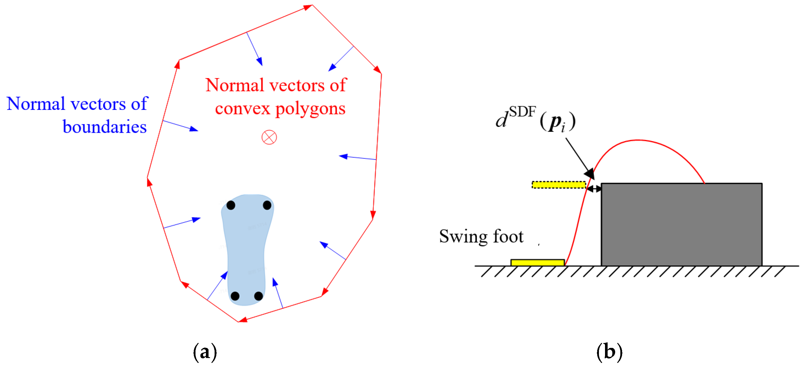
For the four contact points of the supporting leg, each contact point must lie within a three-dimensional space bounded by a convex polygon. This space is enclosed by N boundary surfaces, each of which is perpendicular to the plane of the convex polygon and passes through one edge of the convex polygon, as illustrated in Figure 4a. The condition that the contact points simultaneously lie on the positive side of the N boundary surfaces can be expressed in vector form as follows:

$$h_i^t=A_i^t\cdot p_i+b_i^t\ge 0$$

(23)

where $A_i^t\in {ℝ}^{N\times 3}$ and $b_i^t\in {ℝ}^N$ are the parameters of the boundary surfaces, and p_i is the position vector of the i-th contact point in the inertial coordinate system.

During the swing phase, to prevent collisions between the swinging foot and the environment, a one-dimensional nonlinear inequality constraint is applied to each contact point of the foot, expressed as:

$$h_i^d=d^{\mathrm{SDF}}(p_i)-d_{\min }\left(t\right)\ge 0$$

(24)

where a signed distance field is used to describe the shortest distance from the position of contact point p_i to the obstacle d^SDF(p_i), as shown in Figure 4b, and d_min(t) is a time-dependent shaping function that relaxes this constraint under specific conditions.

To prevent relative sliding between the supporting foot and the environment, a second-order nonlinear inequality constraint is applied to each contact point, expressed as follows:

$$h_i^f={\mu }_c{F}_z-\sqrt{\left(F_x^2+F_y^2+{\epsilon }^2\right)}\ge 0$$

(25)

where μ_c is the friction coefficient, [F_x F_y F_z]^T = ^FR_If_i represents the tangential contact force in the foot coordinate system, and ε > 0 is introduced to ensure the continuity of the constraint derivative when f_i = 0. Additionally, the linear velocity of the contact points should be constrained to zero, i.e., v_i = 0.

During the swing phase, a height trajectory constraint is imposed on the four contact points, expressed as follows:

$$n^T\left(t\right)\left(v_i^{\mathrm{ref}}-v_i+k_p\left(p_i^{\mathrm{ref}}-p_i\right)\right)=0$$

(26)

where p_i^ref and v_i^ref are the reference position and velocity of the i-th contact point, respectively, and k_p is the position error gain. The normal vector $n\left(t\right)\in {ℝ}^3$ of the plane is obtained through time-based interpolation, with the starting point being the terrain normal vector at the lift-off moment and the endpoint being the terrain normal vector at the landing moment.

To fully constrain the motion of the swinging foot, a constraint is imposed on the foot’s orientation angles, expressed as a three-dimensional nonlinear equality:

$$k_p\cdot dis\left(q_i^{\mathrm{ref}},q_i\right)=0$$

(27)

where $q_i^{\mathrm{ref}}\in {ℝ}^4$ is the orientation reference value of the i-th foot, obtained through time-based interpolation and represented using quaternions, and dis(•) is a function that calculates the distance between two quaternions. Additionally, to ensure that the swinging foot does not make contact with the environment, the contact force should be constrained to zero, i.e., f_i = 0.

Throughout the whole motion, all actuated joints are required to satisfy physical constraints on joint positions and velocities, expressed as multidimensional linear inequalities:

$$h_i^j=\left[\begin{array}{c}{q}_{j,ub}-q_j\\ q_j-q_{j,lb}\\ {\dot{q}}_{j,ub}-{\dot{q}}_j\\ {\dot{q}}_j-{\dot{q}}_{j,lb}\end{array}\right]\ge 0$$

(28)

where $q_{j,ub}$ and ${\dot{q}}_{j,ub}$ are the upper limits for joint positions and velocities, respectively, and $q_{j,lb}$ and ${\dot{q}}_{j,lb}$ are the corresponding lower limits.

4. Numerical Optimization

The standard MPC in Equation (19) is derived from a continuous-time formulation and needs to be transformed into a nonlinear optimization problem for a numerical solution. In this section, the direct multiple-shooting method is employed to discretize the continuous optimal control problem into a finite-dimensional nonlinear optimization problem, which is subsequently solved in real-time using sequential quadratic programming.

4.1. Discretization

Within the prediction horizon [t, t + T], the continuous control signal u(t) is discretized to obtain a finite-dimensional decision variable. These nodes $k\in 0,\dots ,N$ define a series of discrete time instants t_k, with the interval between two adjacent instants being $\delta t\approx T/\left(N-1\right)$. A zero-order hold is applied to discretize the control signal u(t). Let x_k = x(k) and u_k = u(k), and by integrating the continuous system dynamics over a time interval $\delta t$, the discrete dynamics can be expressed as follows:

$$f_k^d\left(x_k,u_k\right)=x_k+{\displaystyle {\int }_{t_k}^{t_k+{\delta }_t}{f}^c\left(x\left(\mathrm{\tau }\right),u_k,t\right)} d\mathrm{\tau }$$

(29)

In this work, an explicit second-order Runge–Kutta (RK2) integration method is employed for numerical approximation in simulating the evolution of the continuous system under zero-order hold inputs. After discretization, the loss function and constraints of the NLP can be described by the loss function and constraints at each node, as follows:

$$\begin{array}{ll}\underset{X, U}{\min }& \Phi \left(x_N\right)+{\displaystyle \sum _{k=0}^{N-1}{L}_k\left(x_k,u_k\right)}\\ \mathrm{s}.\mathrm{t}.& x_0=\tilde{x}\\ & x_{k+1}=f_k^d\left(x_k,u_k\right),\forall k\in \left[0,N-1\right]\\ & g_k\left(x_k,u_k\right)=0,\forall k\in \left[0,N-1\right]\end{array}$$

(30)

where X = [x₀^T, …, x_N^T]^T and U = [u₀^T, …, u_N^T]^T represent the sequences of state variables and input variables, respectively. The nonlinear loss function at each node is denoted as L_k, and the constraints are denoted as g_k. By consolidating all variables into a single vector w = [X^T U^T]^T, the above formulation can be summarized as follows:

$$\begin{array}{ll}\underset{w}{\min }& \varphi \left(w\right)\\ \mathrm{s}.\mathrm{t}.& \left[\begin{array}{c}F\left(w\right)\\ G\left(w\right)\end{array}\right]=0\end{array}$$

(31)

where $\varphi \left(w\right)$ represents the loss function, F(w) is the set of initial state constraints and dynamics constraints, and G(w) is the set of all equality and inequality constraints.

4.2. Sequential Quadratic Programming

For nonlinear constrained optimization problems, the SQP method decomposes the original problem into a series of quadratic programming (QP) problems, which are solved iteratively. At each iteration step, a QP problem is solved, where the objective function is a second-order approximation of the Lagrangian function, and the constraints are linear approximations of the original constraints.

The Lagrangian function corresponding to Equation (31) is given by

$$L\left(w,{\mathrm{\lambda }}_F,{\mathrm{\lambda }}_G\right)=\varphi \left(w\right)+{\mathrm{\lambda }}_F^{T}F\left(w\right)+{\mathrm{\lambda }}_G^{T}G\left(w\right)$$

(32)

where λ_F and λ_G are the Lagrange multipliers associated with the dynamics constraints and equality constraints, respectively. By linearizing the constraints and quadratizing the objective function around the current iterative solution w_i, the QP subproblem is formulated as follows:

$$\begin{array}{ll}\underset{\mathrm{\delta }w}{\min }& {\nabla }_w\varphi {\left(w_i\right)}^T\mathrm{\delta }w+{\displaystyle \frac{1}{2}}\mathrm{\delta }{w}^T{B}_i\mathrm{\delta }w\\ \mathrm{s}.\mathrm{t}.& F\left(w_i\right)+{\nabla }_{w}F{\left(w_i\right)}^T\mathrm{\delta }w=0\\ & G\left(w_i\right)+{\nabla }_{w}G{\left(w_i\right)}^T\mathrm{\delta }w=0\end{array}$$

(33)

where B_i is the Hessian matrix of the Lagrangian function, and the optimization variable δw defines the step size update from the current iterative solution w_i. The solution to this QP problem, denoted as δw*, is used as the search direction for the next iteration, yielding the next iterative point w_i+1. The iteration terminates if w_i+1 satisfies the termination criteria to a given precision or if the maximum number of iterations is reached.

5. Whole-Body Motion Control

High-degree-of-freedom humanoid robots must simultaneously address the requirements of multiple tasks during execution. To resolve these challenges, this study employs a whole-body motion control method based on hierarchical optimization. This approach decomposes the control problem into multiple levels according to task priority, addressing task conflicts and constraint conflicts through optimization methods to achieve whole-body coordinated control and enhance the robot’s ability to execute multiple tasks.

5.1. Task Construction

The complete tasks are divided into two layers, as detailed in

Table 1. Task hierarchy and type.

Hierarchy	Task	Type 1
First-layer	Dynamics equations	=
	Foot contact	=
	Contact force	=
	Friction cone	≥
	Joint torque saturation	≥
Second-layer	Linear momentum	=
	Floating-base orientation	=
	Swing foot pose	=
	Arm joint angles	=
	Contact force regularization	=
	Self-collision avoidance	≥
	Joint limits	≥

¹ = represents that the task is formulated as an equality constraint. ≥ represents that the task is formulated as an inequality constraint.

. The dynamics equation, which provides the most fundamental description of the relationship between robot motion and forces, is assigned the highest priority. To prevent physical damage to hardware due to torque saturation, joint torque limits are also considered in the highest-priority tasks. For underactuated systems, the external forces required for motion are entirely derived from the contact forces between the feet and the ground. Maintaining contact between the feet and the ground is a prerequisite for all other tasks, so the foot contact task is also assigned the highest priority. When the feet are in contact with the ground, the friction cone task must be considered, while for the swinging foot, its contact force task must be addressed.

The primary objective of the second-layer tasks is to follow the trajectories (including momentum, joint space angles, workspace poses, and contact force trajectories) generated by the MPC planning module while satisfying the robot’s dynamic and physical constraints. Under the premise of ensuring the first-layer tasks, the robot’s center of mass position and floating base orientation need to be adjusted to achieve the desired motion, i.e., the linear momentum and floating base orientation tasks. When the robot is walking, the pose of the swinging foot must be controlled to track the optimized trajectory. Additionally, to prevent self-collision between the legs during walking, a self-collision avoidance task is incorporated. To avoid exceeding joint position limits during motion, joint limit tasks are also included. The contact force regularization task aims to ensure a reasonable distribution of contact forces, while the arm joint angle task is designed to track the arm joint trajectory.

5.2. Hierarchical Optimization

Each of the aforementioned hierarchical tasks can be described in the following standard form:

$$\left\{\begin{array}{c}Ax-b=0\\ Dx-f\le 0\end{array}\right.$$

(34)

where A is the task matrix, b is the task vector, D is the constraint matrix, and f is the constraint vector. This formulation includes both equality and inequality constraints, which can be structured into a QP form:

$$\begin{array}{ll}\underset{x, v}{\min .}& {‖Ax-b‖}^2+{‖v‖}^2\\ \mathrm{s}.\mathrm{t}.& Dx-f\le v\end{array}$$

(35)

where the optimization variables are x and v, with v being the slack variable for the inequality constraints.

Assume that an optimal solution for the p-th layers of tasks is x*_p and v*_p. When solving the (p + 1)-th layer task, a key principle must be followed: the solution for the (p + 1)-th layer must not violate the equality constraints of the p-th layers, nor should it violate the inequality constraints of the p-th layers. In order to ensure the strict prioritization of tasks [43], the solution of the (p + 1)-th layer can be found in the null space of all higher-priority layers, which is expressed as follows:

$${\mathit{N}}_p={\mathit{N}}_{p-1}\left(\mathit{I}-{\widehat{\mathit{A}}}_p^{\#}{\widehat{\mathit{A}}}_p\right)$$

(36)

where N_p−1 denotes the null space of all layers from layer 1 to p − 1, and $\left(\mathit{I}-{\widehat{\mathit{A}}}_p^{\#}{\widehat{\mathit{A}}}_p\right)$ denotes the null space of the p-th layer. ${\widehat{\mathit{A}}}_p$ equals A_pN_p−1, which describes the task matrix of the p-th layer projected into the null space of all higher-priority layers. ${\widehat{\mathit{A}}}_p^{\#}$ denotes the pseudo-inverse matrix of ${\widehat{\mathit{A}}}_p$.

The solution of the (p + 1)-th layer can be expressed as follows:

$${\mathit{x}}_{p+1}={\mathit{x}}_p^{*}+{\mathit{N}}_p{\mathit{u}}_{p+1}$$

(37)

where u_p+1 denotes an arbitrary vector lying in the row space of N_p. Substituting x_p+1 into the QP problem in the (p + 1)-th layer yields the following:

$$\begin{array}{ll}\underset{{\mathit{u}}_{p+1},{\mathit{v}}_{p+1}}{\min }& {‖{\mathit{A}}_{p+1}\left({\mathit{x}}_p^{*}+{\mathit{N}}_p{\mathit{u}}_{p+1}\right)-{\mathit{b}}_{p+1}‖}^2+{‖{\mathit{v}}_{p+1}‖}^2\\ \mathrm{s}.\mathrm{t}.& {\mathit{D}}_{p+1}\left({\mathit{x}}_p^{*}+{\mathit{N}}_p{\mathit{u}}_{p+1}\right)-{\mathit{f}}_{p+1}\le {\mathit{v}}_{p+1}\\ & {\mathit{D}}_p\left({\mathit{x}}_p^{*}+{\mathit{N}}_p{\mathit{u}}_{p+1}\right)-{\mathit{f}}_p\le {\mathit{v}}_p^{*}\\ & ⋮\\ & {\mathit{D}}_1\left({\mathit{x}}_p^{*}+{\mathit{N}}_p{\mathit{u}}_{p+1}\right)-{\mathit{f}}_1\le {\mathit{v}}_1^{*}\end{array}$$

(38)

The standard QP form for the (p + 1)-th layer task is expressed as follows:

$$\begin{array}{ll}\underset{X_{p+1}}{\min .}& \frac{1}{2}{X}_{p+1}^T{H}_{p+1}{X}_{p+1}+X_{p+1}^T{g}_{p+1}\\ \mathrm{s}.\mathrm{t}.& {\tilde{D}}_{p+1}{X}_{p+1}\le {\tilde{f}}_{p+1}\end{array}$$

(39)

where X^T_p+1 is the optimization variable, H_p+1 is the Hessian matrix, g_p+1 is the gradient vector, ${\tilde{D}}_{p+1}$ is the constraint matrix, and ${\tilde{f}}_{p+1}$ is the constraint boundary.

The recursive process above is summarized in the pseudocode provided in Algorithm 1.

Algorithm 1. Pseudocode of hierarchical optimization algorithm.

Require: $\begin{array}{l}{\mathit{A}}_1,{\mathit{A}}_2,\cdots ,{\mathit{A}}_N\\ {\mathit{b}}_1,{\mathit{b}}_2,\cdots ,{\mathit{b}}_N\\ {\mathit{D}}_1,{\mathit{D}}_2,\cdots ,{\mathit{D}}_N\\ {\mathit{f}}_1,{\mathit{f}}_2,\cdots ,{\mathit{f}}_N\end{array}$ where N is the number of layers

While p from 1 to N do

if p equals 1 then

x*1 and v*1  ←  solving Equation (35)                   ${\widehat{\mathit{A}}}_1={\mathit{A}}_1$

else

${\mathit{N}}_{p-1} \leftarrow \mathit{I}-{\widehat{\mathit{A}}}_{p-1}^{\#}{\widehat{\mathit{A}}}_{p-1}$                   u*p and v*p  ←  solving Equation (38)                   x*p ← x*p−1 + Np−1 u*p                   ${\widehat{\mathit{A}}}_p$$\leftarrow {\mathit{A}}_p{\mathit{N}}_{p-1}$                 ${\mathit{N}}_p \leftarrow {\mathit{N}}_{p-1}\left(\mathit{I}-{\widehat{\mathit{A}}}_p^{\#}{\widehat{\mathit{A}}}_p\right)$

end if

end while

6. Simulation and Results

To validate the effectiveness of the proposed framework, this study leverages the MuJoCo simulation platform to evaluate the locomotion capabilities of a robot (height: 1.5 m, total mass: 48 kg). Our experimental protocol is designed to quantify three critical performance metrics: dynamic stability, robustness under perturbation scenarios, and adaptive capacity in unstructured terrains. The specific experiments conducted include the following:

(a)

Forward walking: This experiment aims to evaluate the robot’s dynamic stability and locomotion efficiency. The robot is tasked with walking forward on a flat surface, and its gait patterns, balance maintenance, and speed consistency are analyzed to evaluate its dynamic performance.

(b)

External force disturbance: This experiment is designed to test the robot’s robustness against external perturbations. External forces are applied to the robot at various points during its motion, and its ability to recover balance and maintain stable locomotion is observed. This test highlights the control framework’s capability to handle unexpected disturbances.

(c)

Complex terrain walking: This experiment aims to evaluate the robot’s adaptability to uneven and challenging terrains. The robot is required to traverse surfaces with varying slopes, steps, and obstacles. Its ability to adjust its gait, maintain stability, and avoid collisions is analyzed to demonstrate its adaptability to real-world environments.

These simulated experiments collectively provide a comprehensive assessment of the robot’s motion control framework, ensuring its effectiveness in dynamic, robust, and adaptive scenarios. The simulation videos are included in the Supplementary Materials.

6.1. Forward Walking

The whole-body motion control algorithm and state estimation operate at a frequency of 500 Hz. The MPC algorithm runs at a frequency of 50 Hz, with a prediction horizon of 1 s and a discrete time step of 0.015 s. The SQP solver [44] based on HPIPM [45] is employed with a convergence tolerance of 1 × 10⁻⁴ and a maximum of one iteration per optimization cycle. To ensure the computational efficiency, three threads are allocated for SQP calculations. The simulation time step is set to 0.002 s. In the absence of external disturbances and on a flat ground surface, the desired velocity of the robot in the X-direction is set to gradually accelerate from 0 m/s to 1 m/s and then decelerate back to 0 m/s.

Figure 5 shows the velocity tracking curve of the robot’s floating base. The robot successfully follows the commanded acceleration, constant velocity, and deceleration processes. The maximum velocity tracking error at 1 m/s is 0.07 m/s, while the velocity fluctuation in the Y-direction remains within 0.05 m/s. Figure 6 displays the joint torque vs. speed curves during the robot’s walking process, providing a basis for motor selection. Throughout the process, the Hip Pitch joint exhibits the maximum torque, approximately 200 Nm. The joint speeds are generally low, all below 4 rad/s.

6.2. External Disturbance

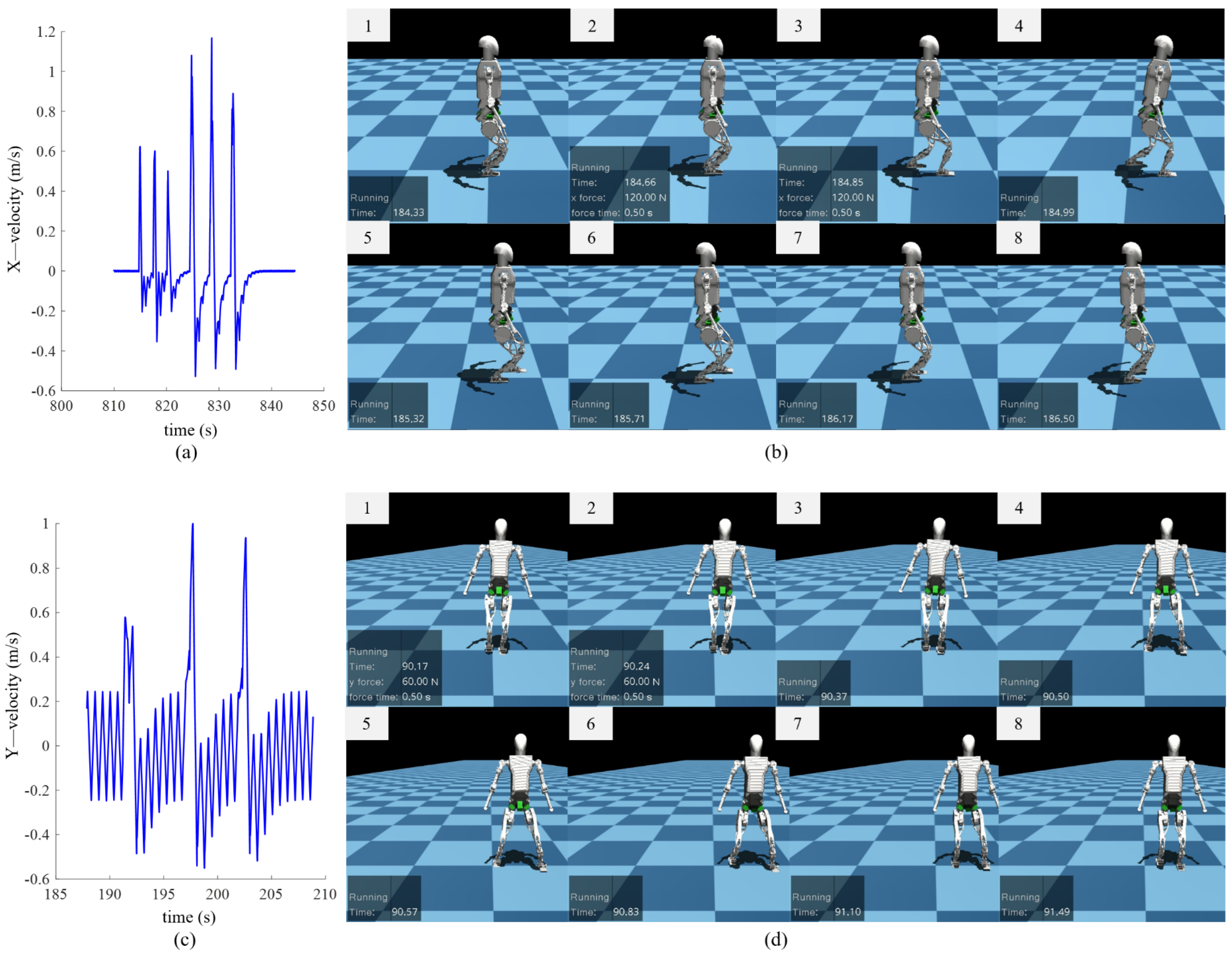
After demonstrating basic walking capabilities, the robot’s stability under external force disturbances is further evaluated. In the simulation environment, the robot is commanded to perform in-place stepping while external disturbances are simulated by applying impulsive forces. The magnitude of the impulsive force is set to 120 N with durations ranging from 0.2 s to 0.5 s.

Figure 7a illustrates the velocity curve of the robot’s floating base. The first three impulsive forces have a duration of 0.2 s, while the latter three have a duration of 0.5 s. It is observed that after experiencing an impulse of 24 Ns, the robot’s velocity exhibits brief fluctuations, with a peak reaching 0.6 m/s. When subjected to an impulse of 60 Ns, the robot’s velocity shows more significant fluctuations, with a peak reaching 1.1 m/s. In this case, the robot adjusts its velocity by taking two consecutive steps forward, as illustrated in the corresponding timing diagram in Figure 7b. The disturbance resistance capability (forward push impulse: 60 Ns, robot mass: 48 kg) demonstrates comparable performance with the learning-based approach implemented on the iCub robot (forward push impulse: 40 Ns, robot mass: 33 kg) [46].

Figure 7c depicts the velocity curve under lateral impulsive forces. Given that the lateral disturbance resistance is weaker than forward resistance, the magnitude of the three lateral impulsive forces is set to 60 N, each with a duration of 0.5 s. It can be seen that after experiencing lateral impulses, the robot’s lateral velocity exhibits substantial fluctuations, with a peak reaching 1 m/s. The robot adjusts its lateral velocity by modifying its lateral foot placement, as shown in the corresponding timing diagram in Figure 7d. Notably, the robot does not exhibit leg crossing after lateral disturbances, validating the effectiveness of the self-collision avoidance constraint in the whole-body control framework.

6.3. Walking Experiments on Complex Terrain

To evaluate the robot’s adaptability to complex terrains, an RGB-D sensor and a staircase terrain were integrated into the simulation environment. The RGB-D sensor was utilized to acquire depth information about the terrain. The staircase consists of four steps, each with a height of 0.16 m and a width of 0.5 m. The elevation map was configured with a size of 3 m × 3 m and a resolution of 0.04 m. The robot was commanded to move forward at a speed of 0.36 m/s with a gait cycle of 0.8 s.

Figure 8a illustrates the timing diagram of the robot climbing the stairs. As the robot approaches the stairs, it autonomously adjusts its base height and modifies its foot placement to align with the step surfaces. To provide a more intuitive representation of the motion details, Figure 8b presents the timing diagram of foot placement planning during the stair-climbing process. In the figure, two robot models are displayed: one representing the current state (with high transparency) and the other representing the 1-second-ahead state (with low transparency). The blue points denote the nominal foot placement points, while the green points represent the projected foot placement points. The swing trajectories of the four contact points are depicted by curves of different colors, and the convex polygonal regions corresponding to the projected foot placement points are represented by polygons of different colors. As shown in Figure 8b, when the nominal foot placement point approaches the edge of a step, the projected foot placement point automatically adjusts to either the current step surface or the next step surface. If the projected foot placement point lies on the next step surface, the swing leg trajectory smoothly transitions from the current step surface to the next, ensuring seamless stair climbing. Simultaneously, the robot’s base height is dynamically adjusted based on the elevation map to align with the step height.

Figure 9 compares the simulation results with and without the swing leg collision avoidance constraint. When the swing leg collision avoidance constraint is not considered, the swing foot trajectory optimized by MPC collides with the stairs (as shown in Figure 9a), resulting in the robot falling. In contrast, when the swing leg collision avoidance constraint is incorporated, the swing foot trajectory optimized by MPC automatically avoids the stair edges (as shown in Figure 9b), ensuring that the swing foot does not collide with the staircase.

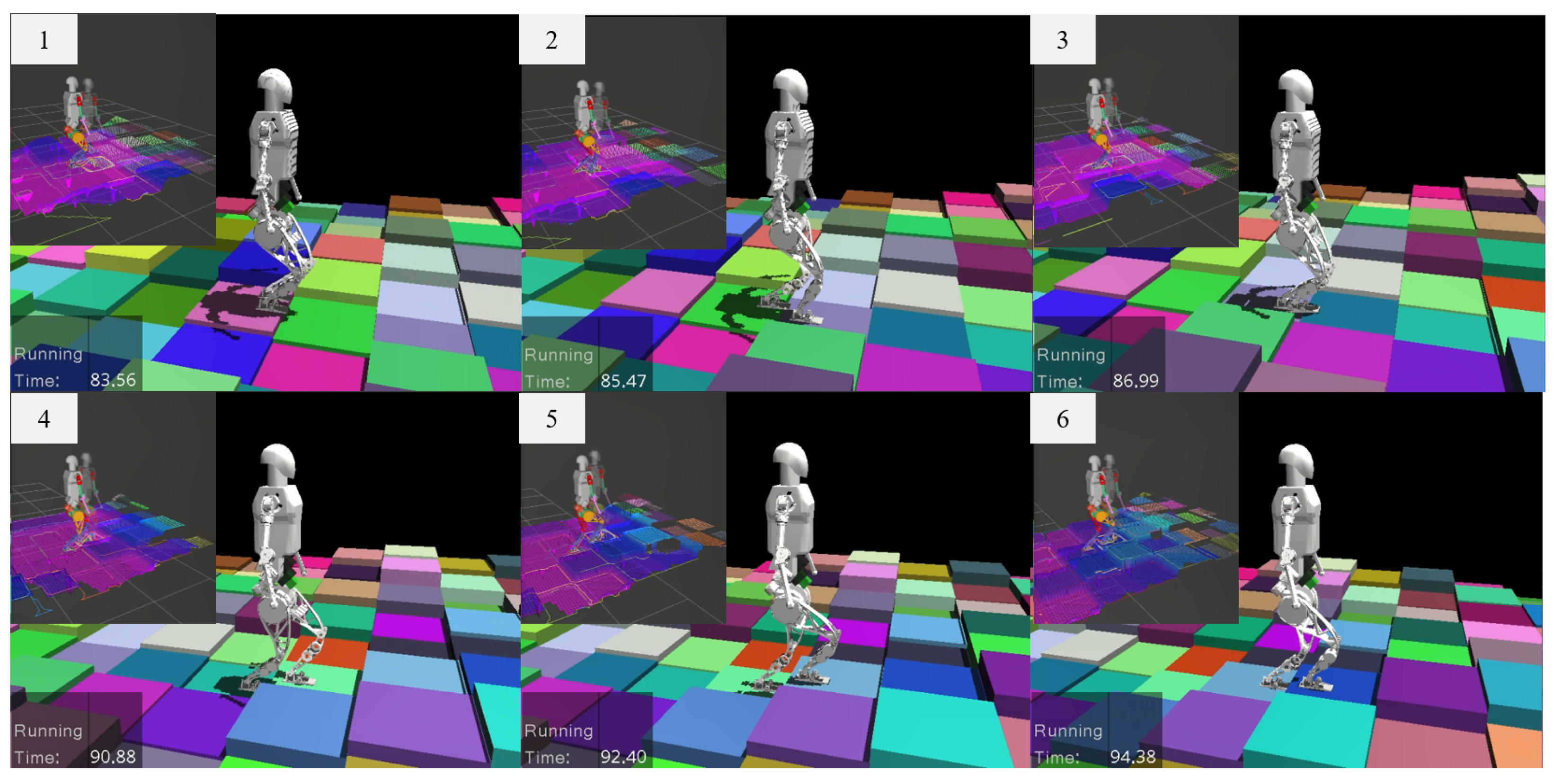
To further evaluate the robot’s terrain adaptability in complex environments, a 20 × 20 grid terrain was constructed in the simulation environment, as illustrated in Figure 10. Each grid cell measures 0.6 m × 0.6 m, with randomly assigned height differences between adjacent grids (up to 0.16 m). For minor height differences, adjacent grids are classified as coplanar regions, enabling direct traversal by the robot. In such scenarios, the robot’s stability is predominantly ensured by the controller’s inherent robustness. Conversely, for significant height variations, foothold planning becomes the critical determinant of successful traversal. Figure 10 illustrates the temporal sequence of the robot navigating this randomized terrain. The results demonstrate that despite stochastic elevation variations between adjacent grids, the robot achieves stable locomotion through adaptive foothold selection and dynamic control.

7. Conclusions

This study has developed a comprehensive terrain-aware hierarchical framework that effectively bridges the perception–planning–control loop for humanoid locomotion in complex environments. By segmenting the elevation map to obtain convex polygonal terrain features, a terrain-constrained nonlinear MPC formulation enabling real-time foothold adaptation through convex polygon constraints is constructed. The sequential quadratic programming algorithm ensures real-time generation of gaits and trajectories with a 50 Hz update rate, while a hierarchical optimization-based whole-body control strategy effectively coordinates dynamic balance and trajectory tracking tasks. The proposed framework has been validated through simulation to significantly enhance the robot’s dynamism, robustness, and terrain adaptability. It provides a novel solution for addressing the challenges of the dynamic motion control of humanoid robots in unstructured environments.

The terrain perception in this work is grounded in elevation mapping techniques, which may introduce inherent limitations when confronting extreme terrains such as sandy substrates, overgrown vegetation, or jagged rocks. It would be hard to extract the convex polygon from these highly irregular geometries or deformable surfaces. Additionally, real-world deployment on physical robots faces challenges, including sensor noise and latency, actuator nonlinearities, and discrepancies between simulated and physical system dynamics. Future investigations are necessary to integrate multimodal perceptions for accurate and robust terrain reconstruction, such as the learning-based method [47], and implement hardware validation to bridge the gap between simulation and real-world deployment.