Abstract
Remaining Useful Life (RUL) prediction is crucial for optimizing predictive maintenance and resource management in industrial machinery. However, existing methods struggle with rigid spatiotemporal feature fusion, difficulty in capturing long-term dependencies, and poor performance on small datasets. To address these challenges, we propose a GPT-based RUL prediction model that enhances feature integration flexibility while leveraging few-shot learning and cross-modal knowledge transfer for improved accuracy in both data-rich and data-limited scenarios. Experiments on the NASA N-CMAPSS dataset show that our model outperforms state-of-the-art methods across multiple metrics, enabling more precise maintenance, cost optimization, and sustainable operations.
1. Introduction
Remaining Useful Life (RUL) prediction serves as a critical enabler for achieving efficient predictive maintenance and resource optimization. Accurately estimating the RUL of mechanical systems can maximize operational efficiency in production lines and control systems, reduce unplanned downtime, enhance product quality, and optimize resource allocation. By precisely assessing the lifespan of mechanical components, industries can proactively identify equipment nearing failure, mitigate unexpected breakdowns, and lower maintenance costs. This capability plays an indispensable role in improving operational efficiency, particularly in high-demand or high-risk industries.
Over the past decades, the significance of RUL estimation has gained widespread recognition, establishing RUL prediction as a core component of Prognostics and Health Management (PHM). Traditionally, industries relied on reactive maintenance strategies—performing repairs only after equipment failure—which often led to abrupt downtime and operational inefficiencies. However, with technological advancements, proactive maintenance has become increasingly vital for reducing operational costs and enhancing equipment availability [1].
The evolution of Predictive Maintenance (PdM) technologies has driven the widespread adoption of machine learning and deep learning models for equipment failure prediction and maintenance optimization [2,3,4]. These methods empower enterprises to forecast failures in advance, optimize downtime scheduling, minimize unnecessary preventive maintenance, and extend equipment uptime while reducing repair costs [5,6]. Furthermore, RUL prediction supports inventory management by enabling timely procurement of replacement parts based on predicted component lifespans, preventing production halts due to critical part shortages.
Deep learning, as a pivotal branch of machine learning, has emerged as a cornerstone technology for RUL prediction due to its capability to autonomously extract features from raw data and perform predictions [7,8,9,10,11]. Despite progress in RUL estimation, challenges persist, particularly in spatiotemporal feature fusion and small-sample learning. Real-world equipment failures often occur infrequently, and the complexity of diverse failure modes complicates data annotation. Additionally, existing models exhibit limitations in flexibly integrating spatiotemporal features from sensor data, struggle to capture long-term dependencies, and underperform on small-sample datasets, collectively exacerbating the difficulty of RUL estimation.
Most feature extraction-based data-driven methods face significant challenges in spatiotemporal feature fusion. Traditional approaches often fuse temporal and spatial features through simplistic operations such as addition or concatenation, which lack flexibility in distinguishing feature importance, thereby compromising feature extraction efficacy. Furthermore, industrial sensor datasets are typically constrained by rare failure events, difficulties in collecting extreme operating conditions, and imperfect data acquisition processes, resulting in insufficient data volume and small-sample datasets. These constraints impose rigorous challenges on model training and generalization capabilities [12,13].
To address these challenges, we propose a novel RUL prediction model integrating spatiotemporal feature fusion with a GPT-based pretrained architecture (DMLP-GPT). The model resolves the inflexibility of traditional feature fusion methods via a dedicated spatiotemporal feature fusion module. By leveraging the few-shot learning capability and cross-modal knowledge transfer of pretrained language models, our approach achieves robust prediction performance under both data-sufficient and data-scarce conditions, significantly enhancing adaptability and robustness.
RUL prediction inherently involves multidimensional monitoring data from diverse equipment, particularly sensor data under varying operating conditions. Current data-driven methods often suffer from rigid feature fusion strategies, especially during spatiotemporal feature extraction [14,15,16]. Conventional fusion techniques, such as additive or concatenative operations, fail to accurately reflect feature importance, thereby degrading prediction accuracy. Moreover, real-world datasets frequently suffer from scarcity due to rare failure modes, extreme operating conditions, or data collection limitations, leading to suboptimal model performance in small-sample scenarios.
To overcome these limitations, this study proposes an RUL prediction framework that combines spatiotemporal feature fusion with few-shot learning capabilities from pretrained language models. First, a flexible feature fusion module is designed to integrate temporal and spatial information effectively, overcoming the limitations of simplistic fusion operations. Second, by leveraging the cross-modal knowledge transfer of pretrained language models, the model compensates for data scarcity through pretrained knowledge, substantially improving prediction accuracy under small-sample conditions.
To validate our approach, experiments are conducted on the NASA N-CMAPSS Turbofan Engine Simulation Dataset. This benchmark dataset, released by NASA, provides comprehensive sensor monitoring data across the full lifecycle of turbofan engines—from healthy states to complete failure—including operational parameters (e.g., altitude, Mach number, throttle resolver angle) and time-series data from 21 critical performance sensors (e.g., temperature, pressure, vibration). High-fidelity simulations replicate engine degradation under diverse operating conditions (e.g., load fluctuations, environmental disturbances) with precise RUL labels, capturing the spatiotemporal heterogeneity of equipment degradation in complex industrial scenarios. Experimental results demonstrate that our model achieves high-precision RUL predictions and maintains superior generalization performance under small-sample training conditions, significantly outperforming state-of-the-art methods.
Key contributions of this study include:
- A spatiotemporal feature fusion module that addresses the inflexibility of existing models in integrating temporal and spatial features, enhancing fusion capability.
- GPT-based pretrained model fine-tuning, leveraging its few-shot learning and cross-modal knowledge transfer advantages, significantly improving RUL prediction performance on small-sample datasets.
2. Related Work
2.1. RNN-Based RUL Prediction
In recent years, there have been significant advancements in Recurrent Neural Networks (RNNs) for Remaining Useful Life (RUL) prediction [9,17]. However, conventional RNN models encounter gradient vanishing/exploding issues when processing long-span temporal sequences, limiting their ability to model long-term dependencies. To address these limitations, Long Short-Term Memory (LSTM) [18,19] and Gated Recurrent Unit (GRU) [20,21] networks have emerged as prominent variants. LSTM employs gating mechanisms to regulate information flow, effectively capturing complex temporal patterns while mitigating long-term dependency challenges [22,23]. GRU achieves comparable performance through a simplified architecture with fewer parameters, offering computational efficiency advantages [24,25]. Both variants demonstrate strong capabilities in equipment RUL prediction, particularly for complex temporal data analysis [26,27].
In practical applications, Liu et al. [18] developed an LSTM framework integrated with statistical process analysis for multi-level feature extraction from vibration signals, outperforming traditional LSTM and Support Vector Regression (SVR) models. Han et al. [19] and Wang et al. [28] enhanced LSTM with attention mechanisms to prioritize critical temporal points. For bearing RUL prediction, Zang et al. [29] optimized LSTM hyperparameters using the Slime Mould Algorithm (SMA), while Zhao et al. [30] combined Bidirectional LSTM (BiLSTM) with attention mechanisms for weighted feature extraction. GRU-based approaches have also shown efficacy: Zhang et al. [20] integrated variational mode decomposition with GRU to leverage time-frequency features, while Xiao et al. [21] improved prediction accuracy through adaptive noise-assisted decomposition methods. She et al. [31] further enhanced model robustness using BiGRU with bootstrap uncertainty quantification. These studies collectively demonstrate that optimized RNN variants achieve robust RUL prediction performance, particularly when augmented with attention mechanisms and decomposition techniques. Nevertheless, existing models still face challenges in flexibly fusing spatiotemporal features from sensor data and capturing long-term dependencies.
2.2. CNN-Based RUL Prediction
The success of Convolutional Neural Networks (CNNs) in computer vision has spurred their adoption for RUL prediction [32]. CNNs excel at extracting localized spatial features through hierarchical convolution and pooling operations, proving particularly effective for equipment fault diagnosis. To adapt CNNs for temporal signal processing, researchers commonly convert sensor data into time-frequency representations using Fourier Transform (FFT) [33] or Continuous Wavelet Transform (CWT) [34,35]. Advanced architectures like ResNet [36,37] and Temporal Convolutional Networks (TCNs) [38,39] further enhance prediction capabilities through residual learning and temporal dependency modeling. Hybrid approaches combining CNNs with complementary methods have demonstrated improved accuracy in complex equipment health monitoring [26,27].
Notable implementations include Ding et al. [33], who combined FFT with CNN for bearing RUL prediction using hierarchical frequency-domain sampling. Yoo et al. [34] achieved 18.96% RMSE reduction on the PRONOSTIA dataset through CWT-based time-frequency image analysis. Wang et al. [35] enhanced empirical wavelet transforms via mutual information for superior performance on both PRONOSTIA and XJTU-SY datasets. Mo et al. [40] developed multi-scale feature fusion with attention weighting, while Zou et al. [41] employed data augmentation to achieve RMSE 0.019 on PRONOSTIA. ResNet adaptations include Mo et al.’s [40] hybrid attention implementation (RMSE/MAE: 0.1079/0.0831) and Wang et al.’s [37] parallel architecture for time-domain/time-frequency feature fusion. Bai et al. [42] combined TCN with CNN for enhanced temporal modeling, while He et al. [38] and Li et al. [39] integrated Graph Convolutional Networks (GCNs) to improve feature robustness. Despite these advancements, current deep learning approaches for RUL prediction still suffer from critical limitations: (1) inflexible fusion of spatiotemporal features in sensor data; (2) difficulties in modeling long-term dependencies; (3) suboptimal performance on small-sample datasets.
3. Proposed Method
The structure of the DMLP-GPT model is shown in Figure 1. The model primarily consists of a spatiotemporal feature extraction module and a GPT pre-trained model. The spatiotemporal feature extraction module is based on a lightweight MLP module, constructing a universal module for preliminary data preprocessing [43,44]. The GPT pre-trained model parameters are then used for the task of predicting the remaining useful life (RUL) of equipment. The model is trained by fine-tuning a subset of the GPT pre-trained parameters.
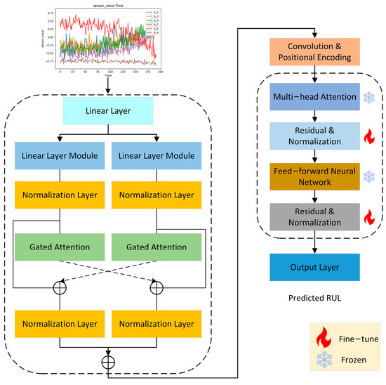
Figure 1.
DMLP-GPT Model Structure.
3.1. Spatiotemporal Feature Extraction Module
The spatiotemporal feature extraction module is divided into temporal and spatial components, as shown in Figure 2. The core distinction between these two parts lies in the dimensions of the input features they process. By applying transpose operations to alter the dimensions of the input data, the model can capture different aspects of the data by processing them along two distinct sets of dimensions.
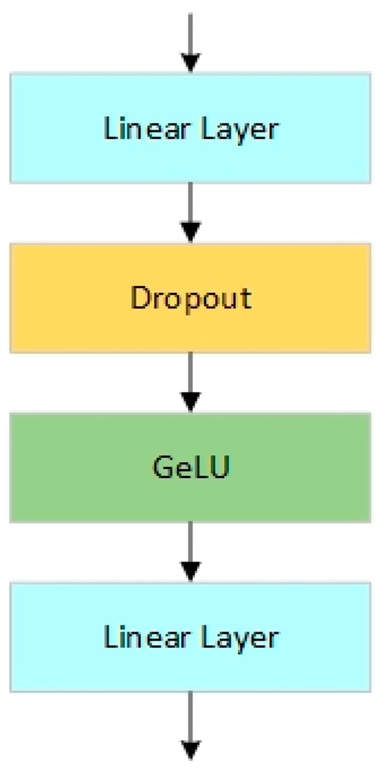
Figure 2.
MLP Module Structure.
The temporal and spatial feature extraction components are primarily based on MLP modules. The interaction and fusion of features between these two parts occur at the black dashed connection lines shown in Figure 1. Similar to residual connections that exchange information along the depth direction of neural networks, these interaction connections facilitate information exchange along the width direction of the neural network. Additionally, to control the feature flow between the two parts, a gated attention module is employed to filter features before fusion.
As shown in Figure 2, the MLP module mainly consists of two linear layers and an activation function. The key formula is:
As shown in Figure 3, the gated attention module filters features by performing a linear transformation and activation function on the input variables, followed by a Hadamard product calculation with the original input. The features filtered by the gating module are solely used for feature exchange and not for subsequent processing within their respective branches. This design prevents gradients from propagating exclusively through the Sigmoid function used in the gating block during backpropagation, thereby mitigating the impact of the gradient saturation regions of the Sigmoid function on the model’s convergence speed.
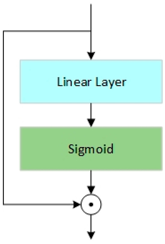
Figure 3.
Gated Attention Module Structure.
The formula is shown below, where denotes the Hadamard product:
3.2. GPT Module
The GPT pre-trained model is primarily composed of decoder modules of the Transformer, as shown in Figure 4.
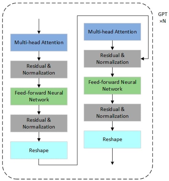
Figure 4.
GPT Model Structure.
Based on existing research in time series forecasting, it has been concluded that the feedforward neural network (FFN) and self-attention modules in the GPT pre-trained model retain most of the learned knowledge. Therefore, during fine-tuning, this study chooses to freeze the FFN and self-attention modules, focusing adjustments on the positional encoding layers and normalization layers to adapt to the RUL prediction task. The overall architecture includes Linear Probing, Patching, Data Embedding Layer, Freezing Pretraining Module, and Output Layer. At the input end, the model extracts time-series features through a data processing layer and converts them into a format acceptable to the GPT-2 model. At the output end, a dedicated prediction layer is added to align with the target dimensions of RUL prediction.
3.2.1. Linear Probing
Linear Probing is an efficient strategy for fine-tuning pre-trained models. Since GPT-2 has already learned rich features during pre-training, this study fine-tunes only the data embedding layer and output layer to minimize training parameters and enhance the model’s generalization capability. The data embedding layer maps time- series data to the input dimensions of GPT-2, while the output layer ensures the final predictions align with RUL requirements.
3.2.2. Patching
To optimize the processing of time-series data, this study adopts a Patching strategy, dividing the input time series into fixed-length segments. The length of each patch is controlled by patch_size, and the step size between adjacent patches is determined by stride. The number of patches, patch_num, can be calculated using the following formula:
where L is the time series window length. This method reduces input sequence length, lowers computational complexity, and enables efficient learning of long-term temporal features.
3.2.3. Data Embedding Layer
To address GPT-2’s limitations in modeling time-series data, positional encoding and value embedding are employed to enhance temporal information. Positional encoding uses sine and cosine functions to preserve temporal dependencies:
where pos denotes the position index, and dmodel represents the embedding dimension. Additionally, the value embedding module transforms input data into feature vectors compatible with the model through convolution operations and dimensionality adjustments.
3.2.4. Freezing Pretraining Module
The FFN and self-attention layers of GPT-2 have learned general features during pre-training. To avoid disrupting this knowledge, these layers are frozen, allowing updates only to parameters in residual connections and normalization layers. This approach reduces trainable parameters and improves the model’s adaptability to small-sample datasets.
3.3. Output Layer
The role of the output layer is to transform the output dimensions of the pre-trained GPT model into the target task’s output dimensions. The formula for the output layer is shown below:
The above formula indicates that the input features undergo a linear transformation through a final linear layer, mapping the extracted features to the prediction label space. This process adapts the model to the downstream task of remaining useful life (RUL) prediction.
3.4. Evaluation Metrics
This study employs two metrics, Mean Squared Error (MSE) and Root Mean Squared Error (RMSE), to evaluate the performance of the proposed model. MSE quantifies the average squared difference between predicted and true values, directly reflecting the model’s prediction error level. RMSE converts the error back to the original scale via square root transformation, providing a more intuitive measure of the actual deviation between predictions and ground truth.
MSE calculates the average of the squared differences between predicted and true values. Its formula is:
where yi is the true value, is the predicted value, and n is the total number of samples. A smaller MSE value indicates lower prediction error.
RMSE transforms the error to the same scale as the original data by taking the square root of MSE. Its formula is:
A smaller RMSE value signifies higher prediction accuracy and stronger interpretability in real-world engineering scenarios.
Compared to a single metric, the combined use of MSE and RMSE provides a comprehensive evaluation of the model’s error distribution characteristics: MSE is more sensitive to outliers, making it suitable for analyzing the absolute magnitude of errors, while RMSE aligns more closely with intuitive error interpretation in practical applications. In industrial predictive maintenance scenarios, the physical significance of RMSE is particularly critical, as it directly guides maintenance strategy formulation and resource allocation optimization.
4. Experimental Results
4.1. Dataset
The experiments utilize the publicly available C-MAPSS (Commercial Modular Aero-Propulsion System Simulation) dataset, proposed by NASA for turbofan engine degradation detection. This dataset collects sensor data from engines during their operational cycles until failure. Each engine’s parameter information includes three operational condition monitoring parameters (flight altitude, Mach number, throttle angle) and 21 performance monitoring parameters.
Table 1 summarizes the basic statistics of the dataset, including the sizes of the training, test, and validation sets. FD001, FD002, FD003, and FD004 are four sub-datasets of C-MAPSS. This study employs FD001 and FD003, two single-operational-condition sub-datasets. FD001 records the operational data of an aircraft engine under high-pressure compressor degradation, while FD003 contains information on two fault modes: high-pressure compressor degradation and fan degradation.
The selection of FD001 and FD003 follows a controlled variable methodology to establish an experimental verification framework. FD001, containing a single fault mode under fixed operational conditions, isolates interference from environmental variables to specifically validate the model’s capability in capturing fundamental degradation patterns. In contrast, FD003 introduces multi-fault coupling scenarios under identical operational conditions, such as simulating synergistic effects between fan wear and lubrication failure, to evaluate the model’s precision in modeling complex fault interaction mechanisms. The performance comparison between the two datasets directly quantifies the impact of fault complexity on prediction errors. The dataset details are shown in Table 1:

Table 1.
Training, Test, and Validation Set Sizes for FD001 and FD003 Datasets.
Table 1.
Training, Test, and Validation Set Sizes for FD001 and FD003 Datasets.
| Dataset | C-MAPSS | |
|---|---|---|
| FD001 | FD003 | |
| Training Set Size | 14,118 | 17,811 |
| Test Set Size | 10,196 | 13,696 |
| Validation Set Size | 3613 | 4009 |
4.2. Data Preprocessing
Figure 5 and Figure 6 illustrate the data distributions of the 21 sensor parameters for the FD001 and FD003 datasets. Based on the distributions, variables with constant values are removed. For example, in the FD001 dataset, sensor variables such as s_1, s_5, s_10, s_15, s_18, and s_19 are excluded.
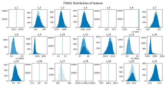
Figure 5.
Data Distribution Histogram for FD001.
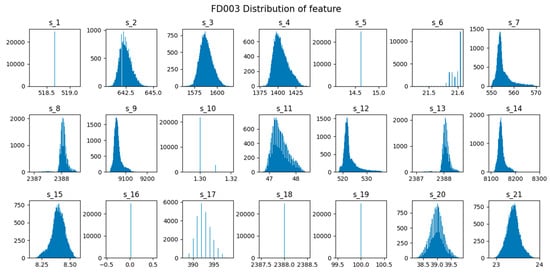
Figure 6.
Data Distribution Histogram for FD003.
Since the data originates from multiple sensors with varying units, standardization is applied to eliminate scale differences between features, improving model convergence speed and accuracy. The standardization formula converts feature data into a distribution with a mean of 0 and a standard deviation of 1:
where x represents the raw feature value, μ denotes the column mean, and σ is the column standard deviation.
This study employs a sliding window approach to construct training samples, ensuring the data captures extensive engine degradation information while mitigating noise and errors. The sliding window size is set to 30, with a stride of 1.
4.3. Experimental Results and Analysis
4.3.1. Comparative Experiments
Under sufficient data conditions, the proposed model is compared with BiGRU_TSAM [45], IMDSSN [46], LSTM [47], and MLP [48] on the C-MAPSS dataset for prediction performance. BiGRU_TSAM employs bidirectional gated recurrent units (BiGRU) for bidirectional temporal modeling, combined with temporal attention mechanisms (TSAM) to dynamically weight critical time-step features, achieving temporal dynamic fusion. LSTM and MLP, as classic baseline models, serve fundamental roles: LSTM captures temporal dependencies via gating mechanisms, while MLP provides basic feature mapping through fully connected layers. The results are shown in Table 2.
Table 2.
Comparison of MSE and RMSE Metrics for Five Models on FD001 and FD003 Datasets.
Table 2 details the performance results of RUL prediction methods on the FD001 and FD003 datasets. In terms of RMSE, our proposed model outperforms others on both datasets, with a more significant improvement on FD003. For example, on FD003, DMLP-GPT achieves an RMSE of 0.0893, representing an 8.2% reduction compared to the next-best method, BiGRU_TSAM. Figure 7 illustrates the prediction results over a full lifecycle in the FD001 test set:
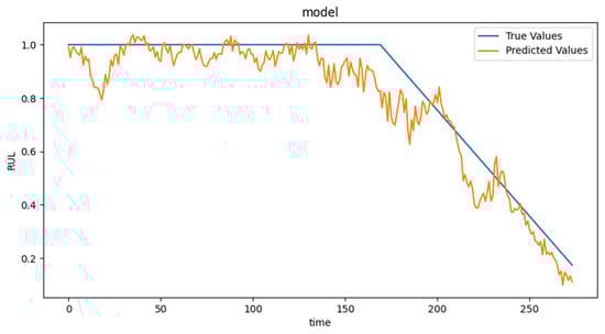
Figure 7.
Line Chart of Prediction Results on FD001 Test Set.
For the few-shot scenario, the training sets are reduced to approximately 15% of their original sizes, while validation and test sets remain unchanged. The revised dataset sizes are summarized in Table 3:
Table 3.
Training, Test, and Validation Set Sizes for FD001 and FD003 (Few-Shot).
The model is compared with BiGRU_TSAM, IMDSSN, LSTM, and MLP on the few-shot FD001 and FD003 datasets. Results are shown in Table 4.
Table 4.
Performance Comparison of Five Models on Few-Shot Datasets (FD001 & FD003).
The table above demonstrates the prediction performance of RUL methods on few-shot datasets. Our model achieves superior results in both MSE and RMSE metrics. For FD001 (few-shot), DMLP-GPT reduces RMSE by 12.3% compared to BiGRU_TSAM and by 32.9% compared to IMDSSN. On FD003 (few-shot), it reduces RMSE by 1.4% compared to BiGRU_TSAM and by 13% compared to MLP. These results validate the effectiveness of our model in few-shot scenarios.
4.3.2. Ablation Study
To investigate the role of the GPT module, an ablation study is conducted by removing the GPT module. Results are shown in Table 5:
Table 5.
Ablation Study Results on FD001 and FD003 Datasets.
The ablation study results presented in the table clearly demonstrate the critical role of the GPT module in the proposed model’s performance. On the FD001 dataset, the removal of the GPT module leads to a moderate increase in RMSE by approximately 0.74%, indicating that even in relatively simple scenarios, the GPT module contributes to improved prediction accuracy. However, the impact becomes significantly more pronounced on the more complex FD003 dataset, where the absence of the GPT module results in a substantial degradation of RMSE by 24.6%. This stark contrast underscores the GPT module’s ability to handle complex, multi-modal data patterns and its effectiveness in capturing long-term dependencies that are crucial for accurate RUL prediction.
5. Conclusions
This study addresses the limitations of existing Remaining Useful Life (RUL) prediction methods, including inflexible spatiotemporal feature fusion, limited long-term dependency modeling, and degraded performance in few-shot scenarios, by proposing the DMLP-GPT framework, integrating spatiotemporal feature fusion with a GPT-based pretrained model. Experimental results demonstrate its superior performance across critical metrics and provide novel insights for industrial equipment health management. Key contributions include:
- Adaptive Spatiotemporal Feature Fusion Module
A gated attention mechanism combined with multi-layer MLP architecture dynamically fuses spatiotemporal features from multidimensional sensor data, overcoming the limitations of traditional additive/concatenative operations.
- 2.
- GPT-Driven Cross-Modal Knowledge Transfer
Leveraging the few-shot learning capability of pre-trained language models, a lightweight fine-tuning strategy (freezing 90% parameters while adjusting positional encodings) achieves an RMSE of 0.1106 with only 15% training data, validating data efficiency.
- 3.
- Robust Long-Term Dependency Modeling
On the NASA C-MAPSS dataset, DMLP-GPT achieves state-of-the-art RMSE (0.0893) and MAE, outperforming benchmarks by 8.2%. Ablation studies reveal a 24.6% RMSE degradation on FD003 when removing the GPT module.
- 4.
- Enhanced Multi-Condition Adaptability
A clustering-based preprocessing method improves the model’s capability to capture heterogeneous degradation patterns in complex industrial scenarios with multi-fault coupling.
Author Contributions
Conceptualization, H.C., X.G. and L.Y.; Investigation, H.C., X.G. and L.Y.; Methodology, H.C., X.G. and L.Y.; Validation, H.C., X.G. and L.Y.; Writing—original draft, H.C.; Writing—review & editing, L.Y. All authors have read and agreed to the published version of the manuscript.
Funding
This work is supported by the National Natural Science Foundation of China under Grant (No. 62171086).
Data Availability Statement
The data presented in this study are available on request from the corresponding author (the data are not publicly available due to privacy).
Conflicts of Interest
The authors declare no conflicts of interest.
References
- Carvalho, T.P.; Soares, F.A.A.M.N.; Vita, R.; Francisco, R.d.P.; Basto, J.P.; Alcalá, S.G.S. A systematic literature review of machine learning methods applied to predictive maintenance. Comput. Ind. Eng. 2019, 137, 106024. [Google Scholar] [CrossRef]
- Serradilla, O.; Zugasti, E.; Rodriguez, J.; Zurutuza, U. Deep learning models for predictive maintenance: A survey, comparison, challenges and prospects. Appl. Intell. 2022, 52, 10934–10964. [Google Scholar]
- Liu, C.-L.; Su, H.-C. Temporal learning in predictive health management using channel-spatial attention-based deep neural networks. Adv. Eng. Inform. 2024, 62, 102604. [Google Scholar]
- Samatas, G.G.; Moumgiakmas, S.S.; Papakostas, G.A. Predictive Maintenance—Bridging Artificial Intelligence and IoT. In Proceedings of the 2021 IEEE World AI IoT Congress (AIIoT), Seattle, WA, USA, 10–13 May 2021. [Google Scholar]
- Sakib, N.; Wuest, T. Challenges and Opportunities of Condition-based Predictive Maintenance: A Review. Procedia CIRP 2018, 78, 267–272. [Google Scholar]
- Polese, F.; Gallucci, C.; Carrubbo, L.; Santulli, R. Predictive Maintenance as a Driver for Corporate Sustainability: Evidence from a Public-Private Co-Financed R&D Project. Sustainability 2021, 13, 5884. [Google Scholar] [CrossRef]
- Liao, X.; Chen, S.; Wen, P.; Zhao, S. Remaining useful life with self-attention assisted physics-informed neural network. Adv. Eng. Inform. 2023, 58, 102195. [Google Scholar]
- Lv, S.; Liu, S.; Li, H.; Wang, Y.; Liu, G.; Dai, W. A hybrid method combining Lévy process and neural network for predicting remaining useful life of rotating machinery. Adv. Eng. Inform. 2024, 61, 102490. [Google Scholar]
- Wang, Y.; Zhao, Y.; Addepalli, S. Remaining Useful Life Prediction using Deep Learning Approaches: A Review. Procedia Manuf. 2020, 49, 81–88. [Google Scholar]
- Deutsch, J.; He, D. Using deep learning-based approach to predict remaining useful life of rotating components. IEEE Trans. Syst. Man Cybern. Syst. 2017, 48, 11–20. [Google Scholar]
- Chen, Z.; Wu, M.; Zhao, R.; Guretno, F.; Yan, R.; Li, X. Machine remaining useful life prediction via an attention-based deep learning approach. IEEE Trans. Ind. Electron. 2020, 68, 2521–2531. [Google Scholar] [CrossRef]
- Aldekoa, I.; del Olmo, A.; Sastoque-Pinilla, L.; Sendino-Mouliet, S.; Lopez-Novoa, U.; de Lacalle, L.N.L. Early detection of tool wear in electromechanical broaching machines by monitoring main stroke servomotors. Mech. Syst. Signal Process. 2023, 204, 110773. [Google Scholar]
- de Lacalle, L.N.L.; Viadero, F.; Hernández, J.M. Applications of dynamic measurements to structural reliability updating. Probabilistic Eng. Mech. 1996, 11, 97–105. [Google Scholar]
- Del Olmo, A.; de Lacalle, L.L.; de Pissón, G.M.; Pérez-Salinas, C.; Ealo, J.; Sastoque, L.; Fernandes, M. Tool wear monitoring of high-speed broaching process with carbide tools to reduce production errors. Mech. Syst. Signal Process. 2022, 172, 109003. [Google Scholar]
- Coro, A.; Macareno, L.M.; Aguirrebeitia, J.; de Lacalle, L.N.L. A Methodology to Evaluate the Reliability Impact of the Replacement of Welded Components by Additive Manufacturing Spare Parts. Metals 2019, 9, 932. [Google Scholar] [CrossRef]
- Sun, S.; Wang, J.; Xiao, Y.; Peng, J.; Zhou, X. Few-shot RUL prediction for engines based on CNN-GRU model. Sci. Rep. 2024, 14, 16041. [Google Scholar] [CrossRef] [PubMed]
- Malhi, A.; Yan, R.; Gao, R.X. Prognosis of defect propagation based on recurrent neural networks. IEEE Trans. Instrum. Meas. 2011, 60, 703–711. [Google Scholar] [CrossRef]
- Liu, J.; Pan, C.; Lei, F.; Hu, D.; Zuo, H. Fault prediction of bearings based on LSTM and statistical process analysis. Reliab. Eng. Syst. Saf. 2021, 214, 107646. [Google Scholar]
- Han, G.J.; Shi, G.H.; Gou, L.F. A Reasoning Network Model for Aero-Engine RUL Prediction. Mini. Micro. Syst. 2022, 43, 1217–1220. [Google Scholar]
- Zhang, Y.; Guan, P. Health status characterization and RUL prediction method of escalator bearing based on VMD-GRU. In Journal of Physics: Conference Series; IOP Publishing: Bristol, UK, 2023. [Google Scholar]
- Xiao, L.; Liu, Z.; Zhang, Y.; Zheng, Y.; Cheng, C. Degradation assessment of bearings with trend-reconstruct-based features selection and gated recurrent unit network. Measurement 2020, 165, 108064. [Google Scholar]
- Li, X.; Li, J.; Qu, Y.; He, D. Semi-supervised gear fault diagnosis using raw vibration signal based on deep learning. Chin. J. Aeronaut. 2020, 33, 418–426. [Google Scholar]
- Jalayer, M.; Orsenigo, C.; Vercellis, C. Fault detection and diagnosis for rotating machinery: A model based on convolutional LSTM, Fast Fourier and continuous wavelet transforms. Comput. Ind. 2021, 125, 103378. [Google Scholar]
- Xiang, W.; Li, F.; Wang, J.; Tang, B. Quantum weighted gated recurrent unit neural network and its application in performance degradation trend prediction of rotating machinery. Neurocomputing 2018, 313, 85–95. [Google Scholar]
- Zhou, J.; Qin, Y.; Luo, J.; Wang, S.; Zhu, T. Dual-thread gated recurrent unit for gear remaining useful life prediction. IEEE Trans. Ind. Inform. 2022, 19, 8307–8318. [Google Scholar]
- Wu, Z. Research on Fault Diagnosis and Prediction Methods for Rotating Machinery and Their Applications. Ph.D. Thesis, Beijing Jiaotong University, Beijing, China, 2016. [Google Scholar]
- Xie, Y.; Zhang, T. A Long Short Term Memory Recurrent Neural Network Approach for Rotating Machinery Fault Prognosis. In Proceedings of the 2018 IEEE CSAA Guidance, Navigation and Control Conference (CGNCC), Xiamen, China, 10–12 August 2018. [Google Scholar]
- Wang, X.; Meng, T.Y.; Zhou, J.X. Remaining Useful Life Prediction of Aero-Engine Based on Attention and LSTM. Sci. Technol. Eng. 2022, 22, 2784–2792. [Google Scholar]
- Zang, C.T.; Liu, R.R.; Yan, H.B. SMA-LSTM-Based Bearing Remaining Life Prediction Method. J. Jiangsu Inst. Technol. 2022, 28, 110–120. [Google Scholar]
- Zhao, Z.; Li, Q.; Yang, S.; Li, L. Research on Remaining Useful Life Prediction Based on BiLSTM and Attention Mechanism. J. Viration Shock. 2022, 41, 44–50+196. [Google Scholar]
- She, D.; Jia, M. A BiGRU method for remaining useful life prediction of machinery. Measurement 2021, 167, 108277. [Google Scholar] [CrossRef]
- Krizhevsky, A.; Sutskever, I.; Hinton, G.E. ImageNet classification with deep convolutional neural networks. Commun. ACM 2017, 60, 84–90. [Google Scholar]
- Ding, H.; Yang, L.; Cheng, Z.; Yang, Z. A remaining useful life prediction method for bearing based on deep neural networks. Measurement 2021, 172, 108878. [Google Scholar]
- Yoo, Y.; Baek, J.-G. A novel image feature for the remaining useful lifetime prediction of bearings based on continuous wavelet transform and convolutional neural network. Appl. Sci. 2018, 8, 1102. [Google Scholar] [CrossRef]
- Wang, W.; Zhao, J.; Ding, G. RUL prediction of rolling bearings based on improved empirical wavelet transform and convolutional neural network. Adv. Mech. Eng. 2022, 14, 16878132221106609. [Google Scholar] [CrossRef]
- Mo, R.P.; Li, T.M.; Si, X.S. Equipment Remaining Useful Life Prediction Method Using Residual Network and Convolutional Attention Mechanism. J. Xi’an Jiaotong Univ. 2022, 56, 194–202. [Google Scholar]
- Wang, X.; Qiao, D.; Han, K.; Chen, X.; He, Z. Research on predicting remain useful life of rolling bearing based on parallel deep residual network. Appl. Sci. 2022, 12, 4299. [Google Scholar] [CrossRef]
- He, K.; Su, Z.; Tian, X.; Yu, H.; Luo, M. RUL prediction of wind turbine gearbox bearings based on self-calibration temporal convolutional network. IEEE Trans. Instrum. Meas. 2022, 71, 3501912. [Google Scholar] [CrossRef]
- Li, P.; Liu, X.; Yang, Y. Remaining useful life prognostics of bearings based on a novel spatial graph-temporal convolution network. Sensors 2021, 21, 4217. [Google Scholar] [CrossRef] [PubMed]
- Mo, R.P.; Si, X.S.; Li, T.M.; Zhu, X. Bearing Life Prediction Based on Multi-Scale Features and Attention Mechanism. J. Zhejiang Univ. Eng. Sci. 2022, 56, 1447–1456. [Google Scholar]
- Zou, W.; Ji, C.; Chen, W.X.; Zheng, K. Multi-Bearing Remaining Life Prediction Based on Data Augmentation and Convolutional Neural Network. J. Mech. Des. 2021, 38, 84–90. [Google Scholar]
- Bai, S.; Kolter, J.Z.; Koltun, V. An empirical evaluation of generic convolutional and recurrent networks for sequence modeling. arXiv 2018, arXiv:1803.01271. [Google Scholar]
- Ekambaram, V.; Jati, A.; Nguyen, N.; Sinthong, P.; Kalagnanam, J. Tsmixer: Lightweight mlp-mixer model for multivariate time series forecasting. In Proceedings of the 29th ACM SIGKDD Conference on Knowledge Discovery and Data Mining, Long Beach, CA, USA, 6–10 August 2023. [Google Scholar]
- Chen, S.A.; Li, C.L.; Yoder, N.; Arik, S.O.; Pfister, T. Tsmixer: An all-mlp architecture for time series forecasting. arXiv 2023, arXiv:2303.06053. [Google Scholar]
- Zhang, J.; Tian, J.; Li, M.; Leon, J.I.; Franquelo, L.G.; Luo, H.; Yin, S. A Parallel Hybrid Neural Network With Integration of Spatial and Temporal Features for Remaining Useful Life Prediction in Prognostics. IEEE Trans. Instrum. Meas. 2023, 72, 3501112. [Google Scholar] [CrossRef]
- Zhang, J.; Li, X.; Tian, J.; Luo, H.; Yin, S. An integrated multi-head dual sparse self-attention network for remaining useful life prediction. Reliab. Eng. Syst. Saf. 2023, 233, 109096. [Google Scholar] [CrossRef]
- Sayah, M.; Guebli, D.; Al Masry, Z.; Zerhouni, N. Robustness testing framework for RUL prediction Deep LSTM networks. ISA Trans. 2021, 113, 28–38. [Google Scholar] [PubMed]
- Tolstikhin, I.O.; Houlsby, N.; Kolesnikov, A.; Beyer, L.; Zhai, X.; Unterthiner, T.; Yung, J.; Steiner, A.; Keysers, D.; Uszkoreit, J.; et al. Mlp-mixer: An all-mlp architecture for vision. Adv. Neural Inf. Process. Syst. 2021, 34, 24261–24272. [Google Scholar]
Disclaimer/Publisher’s Note: The statements, opinions and data contained in all publications are solely those of the individual author(s) and contributor(s) and not of MDPI and/or the editor(s). MDPI and/or the editor(s) disclaim responsibility for any injury to people or property resulting from any ideas, methods, instructions or products referred to in the content. |
© 2025 by the authors. Licensee MDPI, Basel, Switzerland. This article is an open access article distributed under the terms and conditions of the Creative Commons Attribution (CC BY) license (https://creativecommons.org/licenses/by/4.0/).