Automated Selection of Time Series Forecasting Models for Financial Accounting Data: Synthetic Data Application

Abstract

The continuous forecasting of anticipated trends in company accounting helps to prepare for possible challenges and investment possibilities. The forecasting of performance indicators for each partner and metric in a company requires a high volume of resources, as each forecasting model requires some supervised adjustment. To solve the challenge of manual work in this task, AutoML solutions can be used. In this study, we propose an automated forecasting model selection option. The time series data are summarized by 21 statistical features and different experiments are performed to find the best-suited forecasting method. Different classifier models are tested with the dataset, estimating the impact of data sampling and synthetic data generation. The results indicate that the undersampling approach is more suitable, as it helps in balancing the classes. Random forest methods usually show the best performance, achieving about 74% accuracy. The usage of a synthetic data-based dataset for model training reduced the accuracy by almost 20%, while the integration of synthetic and real time series data allowed us to achieve balance between both classes. This confirms that synthetic time series data generation might increase the accuracy of forecasting method selection, but it should be used in combination with real data.

1. Introduction

Data analytics and forecasting have become an important part of business management [1]. Artificial intelligence (AI) and machine learning (ML) methods are applied to analyze available data, and based on this, to predict upcoming results, possible risks, etc. In the current state, general AI is already capable of performing some common data analysis for financial tasks [2], but more specific models are used for certain data analysis and prediction tasks. This allows for more accurate model results to be obtained. However, building such an AI model requires experts to work to adjust the model or to conduct systematic experiments to analyze all possible model parameters and feature sets to find the most suitable configuration. In both cases, building an accurate AI model requires a good quality dataset and time [1,2]. The task of forecasting company financial accounting data for each client does not provide any of these resources. The following requirements and limitations apply to this task:

• Companies have multiple clients with different collaboration patterns. Building one model to fit all clients is not feasible, considering the data variety of clients’ collaboration patterns.
• The financial accounting data for each client have a set of monitored features (number of sales/purchases, amount, delays, discounts, etc.). The development of separate AI models for each client and each relevant financial accounting data feature would lead to an enormous number of models and consequently model building efforts.
• New clients are coming and going; therefore, in the case of one AI model, it should be retrained or fine-tuned to reflect the collaboration pattern of the client. Otherwise, a new AI model or models have to be developed for this client specifically.
• Forecasting tasks are very “live”, as data are changing constantly. This requires new model training after each data update.
• The landscape of data forecasting models and their parameters is wide. The selection of a suitable method and the grid search of its parameters might be too costly and slow.

Automated Machine Learning (AutoML) is used to overcome these limitations and challenges. These are methods and processes designed to automate the application of machine learning in real-world situations [3]. The automation can include steps such as collecting and processing the dataset, selecting the model and tuning its parameters, and evaluating the results.

The main objective of this research is to automate the forecasting of financial accounting data for each company client and the monitored financial accounting data fields. This reflects a real situation when companies want to forecast different features for the selected clients and an AutoML solution is needed. They do not have time to manually build separate forecasting models when the forecast is needed immediately to make decisions on further steps. Therefore, we aim to reduce the data forecasting model selection time by proposing a model data forecasting method, which would allow companies to fully automate data forecasting, keeping the needed forecast accuracy.

This paper is oriented on two main research questions:

• How does the utilization of synthetic data affect the data forecasting prediction method selection accuracy?
• How accurately can the best forecasting method be predicted based on time series descriptive data?

To answer the research questions, in Section 2 we review the related work. Then, Section 3 summarizes the forecasting method prediction experiments with the existing dataset. The dataset, classification model selection, and the obtained results are presented there. Section 4 describes the dataset augmentation solution we propose and investigates the effect of different dataset balancing options. Section 5 and Section 6 summarize the research.

2. Related Work

Data forecasting involves predicting the future values of a specific variable based on historical data [4]. Typically, this forecasting is performed for a single variable, considering only its past values and excluding additional variables. Such data forecasting is commonly referred to as time series forecasting. The choice and application of existing data forecasting methods for financial accounting data can vary significantly, so understanding the different types and their unique characteristics is crucial.

One of the earliest approaches to time series forecasting was through stochastic methods [5]. Stochastic models make assumptions about the underlying process and associated probability distributions [6]. These models perform well when data changes are not overly complex, and the initial conditions meet the stationary assumption. Examples of stochastic time series forecasting models include VAR, ARIMA, and ARIMAX models [7], with variations proposed for seasonal data (such as SARIMAX [8]).

However, the requirement for data to be stationary limits the applicability of these models. Exponential smoothing is a solution for non-stationary data [9]. One such model is the Damped Local Trend (DLT) model, which supports linear, log-linear, and logistic deterministic global trends, along with a regression component.

For handling non-stationary data, artificial intelligence methods come into play [10]. Common AI models in this context include Support Vector Machine (SVM), Naive Bayes, Decision Tree, Multilayer Perceptron (MLP), Recurrent Neural Network (RNN), and Long Short-Term Memory (LSTM) [11]. Among these, LSTM is widely used for general-purpose time series forecasting due to its ability to address the vanishing gradient problem [12].

Despite the effectiveness of these models, manually building a data forecast for every client a company collaborates with can be impractical due to the workload on data analysts. Automation is essential to transition toward adaptive data forecasting models or automated model development.

To assist data analysts in building accurate data forecasts and prediction models, additional solutions are available. Algorithm selection and hyperparameter optimization fall under the umbrella of Automated Machine Learning (AutoML) [13]. Existing AutoML tools (such as auto-sklearn [14], TPOT [15], ML-Plan [16], Auto-WEKA [17], and others) test various models with different hyperparameters to find the best fit. As the performance and application requirements dictate, AutoML is gaining traction.

Research papers explore AutoML applications in diverse fields, including healthcare [18], video analytics [19], manufacturing [20], and telecommunications [21]. In finance and accounting, Agrapetidou et al. [22] demonstrated that AutoML can enhance financial data analysts’ productivity by automating bank failure forecasts. However, further research is needed to fully unlock AutoML’s potential and reduce the cost of building forecast models, especially in scenarios requiring numerous individual models.

For higher forecasting automation, zero-shot forecasting models have arisen during the last few years [23,24]. The ForecastPFN solution [23] is based on building a large time series forecasting model based on synthetic data. The trained model is then used for the forecast of the input data to achieve the prediction. Some solutions [24] adapt large language models for time series forecasting by encoding numerical values into numerical digits. Such solutions indicate promising results and a very high level of automation, while at the same time, their limitation is the need for the large model and dataset it requires.

In the area of time series data augmentation and synthetic data generation, multiple initiatives exist. In some cases, the time series are used for anomaly detection [25] and fault diagnosis [26]. These situations require additional data for the rare cases but keep a similar pattern of data. In this case, noise adding is more effective, rather than the generation of synthetic data. While different time series application areas exist, the data augmentation of time series always tries to take into account the existing data and extend it, rather than generate new patterns [27].

Generating a new time series is common as well, but is usually closely related to a specific area. For example, in medicine [28] and edge computing [29] synthetic time series data can be generated to reflect real signals. Such a situation requires the real signals to be mimicked and they are usually based on some theoretical model or the identification of the existing time series properties. Generating new time series data for unknown patterns might be complicated. Recently, some tools were introduced for time series data generation [30], but the main metric for a generated time series is usually human evaluation and quality estimation.

To combine the benefits of traditional forecasting methods and the requirement for limited resource usage, a two-shot approach could be utilized. In the first step, the most suitable forecasting model would be selected, while the second step would produce the output of the selected model.

3. Model for Company Financial Accounting Data Forecasting Method Selection

3.1. Company Financial Accounting Data

For the automated data forecasting model selection, accounting data from four companies were collected. All four companies were located in Lithuania; however, their activity and size varied, and foreign customers existed among their clients. The accounting data were selected from the year when the companies started using the accounting system and had a full year of accounting records available. The data from the accounting system was aggregated by month (to reflect the traditional accounting period), reflecting the culminative values of 23 features, indicating the count of invoices, products, the sum of purchase, selling costs, delays in payment, discounts, etc. For further experiments, only the sum of purchase costs for each month were used, forming a data file for each collaborating company and presenting records for each month. This field was selected as the main one, illustrating the possible income in the company. In addition, it was the most common non-zero-value-containing field. The data field was used as the time series data and the main idea was to forecast its values using univariate forecasting methods for the next year ahead.

The summarized numbers of the initial dataset used are presented in

Table 1. Summary of company data used as initial dataset.

Company ID	No. of Clients	Record From	Record Until	No. of Non-Zero Records	Percentage of Non-Zero Months
#1	196	2012 January	2020 December	8682	41% (stdev = 0.25)
#2	698	2015 January	2020 December	3884	8% (stdev= 0.15)
#3	140	2017 January	2020 December	3930	58% (stdev = 0.29)
#4	21	2015 January	2020 December	834	55% (stdev = 0.33)

. They illustrate that company #2 is more oriented on short, non-recurrent orders as it has the biggest number of clients, while having the smallest relative number of non-zero records (only 8% of months in the history of collaboration have non-zero values). Meanwhile, about half of the records of all other companies have non-zero values, but the variation in the constant collaboration is very high (the standard deviation is more than 0.25).

The data are not very systematic, as none of the companies have many strongly connected clients which purchase something every month. From the dataset, company #2 had two clients which purchased something in all 72 months in the analyzed period. Companies #1 and #4 had only one company which purchased something every month, while company #3 had no such companies.

3.2. Experimental Environment

The research experiments were conducted using the KNIME 5.4.3 platform and JupyterLab environment for Python 3 programming, using various Python libraries and packages. Python was used to build the dataset for the forecasting method selection: the statsmodels package was used to analyze the time series and forecast with the SARIMA model, the Orbits package was used for the DLT forecasting model, and the Keras library from Tensorflow library was used to implement the LSTM model. The KNIME platform was used to model different situations and investigate the suitability of the classifiers for the selection of the prediction model.

3.3. Dataset for Forecasting Method Selection

The purpose of this research was to predict which data forecasting model would work best for specific time series data from company accounting data. The original dataset was not suitable for use as an input for the model because it had to be presented as one record with fixed features. Therefore, from the obtained initial dataset, a new dataset was built. To build the dataset, we took the 1055 data files representing each client of the companies. Records with at least 12 non-zero values in the clients’ time series were selected as part of the next dataset. This left only 424 files/records and was performed to eliminate mostly inactive collaboration cases, where mostly constant zero values were present.

The time series were summarized into 21 features (quantity of monthly records, min. value, max. value, mean value, standard deviation, lower quartile, median, upper quartile, annual correlation coefficient, augmented Dickey–Fuller test value, p-value, critical values for augmented Dickey–Fuller test statistic at 5% and 10%, augmented Dickey–Fuller test value after first order differencing, p-value after first order differencing, critical values for augmented Dickey–Fuller test statistic at 5% and 10% after first order differencing, augmented Dickey–Fuller test value after first order differencing and third-degree root transformation, p-value after first order differencing and third-degree root transformation, and critical values for augmented Dickey–Fuller test statistic at 5% and 10% after first order differencing and third-degree root transformation), reflecting the statistical features of the time series.

At the same time, the normalized time series data were used to find the best forecasting model. For each of the files, three time series forecasting methods were used using the AutoML option, where, in total, 659 combinations of their parameters were applied to achieve the least RMSE value for the next 12 months [31]. As a result, the LSTM model was the most suitable (with the lowest RMSE value) in 319 cases out of 424. SARIMA showed the smallest error in 105 cases. While DLT was never better than other methods, it sometimes demonstrated the same lowest accuracy as the SARIMA method (mostly in cases of constant zero values). In this way, we achieved a new dataset composed of 424 records. The process of building the dataset is presented in Figure 1.

The number of records obtained in the dataset was relatively small to try to achieve a very high accuracy. To estimate what the accuracy of the forecasting method prediction could be, the initial experiments were executed.

3.4. Forecasting Method Selection Performance

Business recommendation systems are characterized by a large number of clients. For each of them, a recommendation model needs to be developed, and therefore also a classification model. The classification model cannot be complex without overloading the servers/system processes. Therefore, in this paper, traditional machine learning algorithms were chosen: k-NN, Naïve Bayes, SVM, MLP, PNN, random forest, and gradient boosted trees. For the same reasons, the parameterization options of the algorithms were constrained. The analyzed parameters are listed in

Table 2. Parameters for the forecasting method prediction.

Classification Method	Parameter	Parameter Values
		Start	End	Step
k-NN	k	3	10	1
SVM	c	0.01	100	0.1
Naïve Bayes	Max. number of norm. values	20	100	1
MLP	Iterations	20	200	00
	Layers	1	5	1
	Neurons	8	100	2
PNN	Theta plus	0.4	1	0.1
	Theda minus	0.1	0.4	0.1
random forest	Trees	10	200	10
	Tree depth	5	50	1
gradient boosted trees	Trees	10	200	10
	Tree depth	5	50	1

.

The research was carried out in two cases: with an imbalanced dataset (424 records) and with a dataset balanced towards the smaller SARIMA class (210 records). The oversampling option was not analyzed, as it would generate synthetic data and would not reflect a real situation where only real data are used.

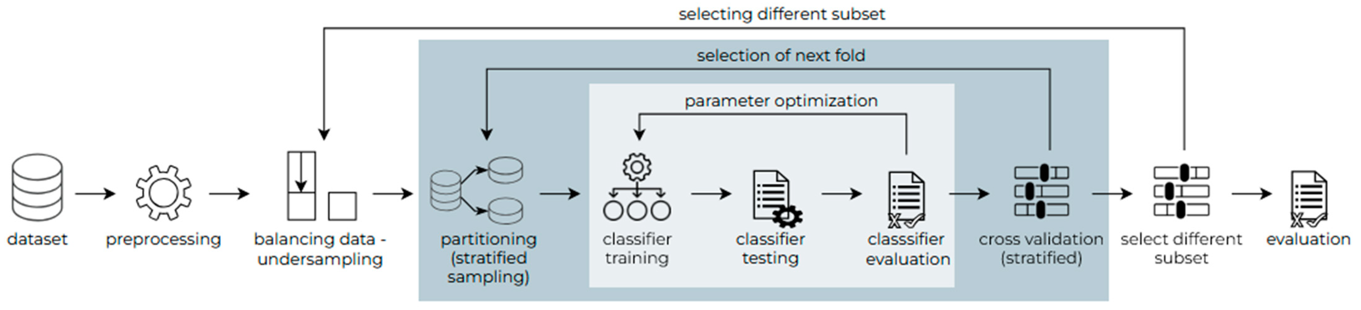
The flowchart for the research on the imbalanced dataset can be seen in Figure 2. The dataset consisted of 424 records, of which 105 were SARIMA and 319 were LSTM. The data were min–max normalized and split by 20%/80% to train and test the classifiers. Five-fold cross validation was applied to maximize the accuracy of the results. The whole process was repeated five times.

In the case of undersampling, a subset of LSTM was randomly selected so that the size of the two classes was the same: 105 SARIMA and 105 LSTM. The methodology was the same as in the imbalanced case and the research was repeated five times, each time selecting a different subset of the LSTM class dataset (see Figure 3).

The parameters that were optimized for each model can be seen in

Table 3. Evaluation of forecasting method classifiers with original dataset.

	Classifiers	Average Acc.	Best Case Metrics
			Classes	Recall	Precision	F1	Parameters
Imbalanced	k-NN	0.755	LSTM	0.830	0.772	0.800	k = 3
			SARIMA	0.257	0.333	0.290
	SVM	0.752	LSTM	1.000	0.752	0.858	c = any value
			SARIMA	0.000	0.000	0.000
	Naïve Bayes	0.366	LSTM	0.206	0.808	0.329	56 max number norm. val.
			SARIMA	0.847	0.260	0.398
	MLP	0.776	LSTM	0.915	0.800	0.853	138 iter., 3 layers, 60 neurons
			SARIMA	0.304	0.542	0.390
	PNN	0.774	LSTM	0.956	0.776	0.856	theta plus 0.573, theta minus 0.105
			SARIMA	0.161	0.548	0.250
	random forest	0.778	LSTM	0.968	0.786	0.867	54 trees, 17 tree depth
			SARIMA	0.200	0.677	0.308
	gradient boosted trees	0.767	LSTM	0.774	0.817	0.795	91 trees, 50 tree depth
			SARIMA	0.476	0.409	0.440
Undersampled	k-NN	0.585	LSTM	0.695	0.603	0.646	k = 4
			SARIMA	0.542	0.640	0.587
	SVM	0.584	LSTM	0.314	0.733	0.440	c = 0.456
			SARIMA	0.885	0.563	0.688
	Naïve Bayes	0.537	LSTM	0.676	0.554	0.609	72 max number norm. val.
			SARIMA	0.457	0.585	0.513
	MLP	0.630	LSTM	0.647	0.647	0.647	47 iter., 3 layer, 88 neurons
			SARIMA	0.647	0.647	0.647
	PNN	0.611	LSTM	0.619	0.656	0.637	theta plus 0.847, theta minus 0.392
			SARIMA	0.676	0.639	0.657
	random forest	0.615	LSTM	0.647	0.653	0.650	101 trees, 30 tree depth
			SARIMA	0.657	0.650	0.654
	gradient boosted trees	0.650	LSTM	0.704	0.672	0.688	199 trees, 6 tree depth
			SARIMA	0.657	0.690	0.673

. It indicates that in the case of the imbalanced dataset, all the classifiers learned to mostly predict the LSTM class (except for the Naïve Bayes, which learned to predict only the SARIMA class). In the case of the undersampled dataset, gradient boosted trees and MLP showed the best results.

Taking into account that there were only two classes, the classification accuracy could have been higher. In the case of imbalanced data, the average accuracy was higher than in the case of undersampling (reached 78% in comparison to the maximum of 65% accuracy). However, the high differences in recall between each class made the classifiers unreliable. Therefore, attempts have been made to improve it by adding synthetic data to the dataset.

4. Synthetic Data Generation for Dataset Extension in Forecasting Method Selection

4.1. Synthetic Data Generation Method

The real dataset is rather small and unbalanced, which makes it difficult to train classification models. Real client data are characterized by an abundance of zero: only 28 clients have a minimum data value that is not zero, and at least 25% of the data are zero for 333 out of 425 clients. Most of the real client data shows poor seasonality too. For these two reasons, it is decided to generate synthetic client data with non-zero values and add records with annual seasonality.

The augmentation of the real time series is not the best option in this case, as it would mimic the existing patterns but would not introduce a new one. This way, the augmented dataset usage would potentially lead to overfitting of the model and would not work for newly added time series patterns. Therefore, the approach to generate at least some common pattern data is selected.

Traditionally, adding synthetic data to the dataset might incorporate bias or distortions that are not common in real data. Therefore, the data augmentation and generation must be performed with high attention and validation. Existing research [32] indicates that the usage of time series data augmentation can significantly increase forecast accuracy; however, it is very dependent on using data augmentation methods, dataset size, and situation specifics.

In this research, the forecasting method selection uses preprocessed time series data, not the time series itself. Based on the estimated features of the time series, the classification model estimates under what properties of the time series one or another time series forecasting model would potentially be the most suitable. To avoid the generation of the classification model training data, we generate time series, which are used to model different situations and to estimate which method is the most accurate for its data forecasting. In this way, the classification model dataset is real, obtained by multiple modelling activities, and not generated. Only the data used to obtain the dataset is synthetic.

Usually, a time series signal can be expressed in three components: seasonality, trend, and noise. Taking into account the fact that the interaction between them is additive, the signal can be expressed as:

$$Y_t=f\left(S_t,T_t,N_t\right)=S_t+T_t+N_t,$$

(1)

where $Y_t$ is the time series signal at time t, $S_t$—seasonality, $T_t$—trend, and $N_t$—noise.

Different seasonality and trend cases were generated for the synthetic dataset, while in all cases, the same red noise [33] function—noise serially correlated in time, in other words, noise with memory—was used to define the noise. The noise was used to reflect possible variations in the time series data, which could rise in real life (accounting delays, change in supply chain, economics, etc.).

The red noise parameters were chosen during all synthetic data generations as follows: variation was randomly chosen between 0.01 and 0.3 and multiplied by the trend base, and correlation was randomly chosen between 0.7 and 0.99. A relatively small noise variation was chosen because a larger variation would obscure the signal and make it unpredictable. A high correlation was chosen to better match real data. The exact ranges of the parameters were determined by manual experimental tests to reflect various but still similar to realistic conditions.

For the dataset extension with synthetic data, 900 different time series were generated. For the signal generation, the mokseries library was used [34]. To reflect different patterns of the time series, several strategies were used:

• A total of 60 synthetic time series were generated without seasonality and with an exponential trend and red noise, including different a and b parameter values to reflect the exponential trend by the function

$$Y_t=a^t+b+N_t,$$

(2)

• A total of 300 synthetic time series were generated without seasonality and with a linear trend and red noise, including different a and b parameter values to reflect the linear trend by the function

$$Y_t=a\times t+b+N_t,$$

(3)

• A total of 300 synthetic time series were generated with sinusoidal yearly seasonality, a linear trend, and red noise, including different k parameter values to reflect the amplitude of seasonality and different parameter a and b values to reflect the linear trend by the function

$$Y_t=k·\sin \left(t\right)+a·t+b+N_t,$$

(4)

• A total of 240 synthetic time series were generated with yearly periodic seasonality, a flat trend, and red noise, including different parameter b values to reflect the trend by the function

$$Y_t={S[1\dots 12]}_t+b+N_t,$$

(5)

The selected functions for synthetic data generation allowed different time series patterns to be reflected, while variations in each of the time series cases provided a better distribution of the extended dataset.

4.2. Description of Synthetic Time Series Generation Situations

Each of the four strategies for synthetic time series generation are detailed below, explaining how the parameter values were selected for the dataset extension.

4.2.1. Time Series Without Seasonality and with an Exponential Trend and Red Noise

To reflect the exponential trend, both increasing and decreasing trends were modelled. The list of parameters and their values is summarized in

Table 4. List of parameters and their values for time series generation with no seasonality and with an exponential trend and red noise.

Quantity of Synthetic Client Data	Trend Factor (a)	Trend Base (b)	The Length of One Client Dataset
10	random (1.01, 1.1)	180 + random (−100, 0)	108 (9 years × 12 months)
10			72 (6 years × 12 months)
10			48 (4 years × 12 months)
10	random (0.7, 0.95)	6263 + random (−1124, 1124)	108 (9 years × 12 months)
10			72 (6 years × 12 months)
10			48 (4 years × 12 months)

.

For an exponentially increasing trend, the trend base value was set to 180 because it was the average of the minimum values of the real client data. Analogously, in the case of an exponentially decreasing trend, 6263 was the average of the maximum values of the real client data. The average of the standard deviations of the real data was 1124 and was intended to diversify the data (a random number between −100 and 0 is used in the case of an exponentially increasing trend, so that the values are not less than 0 and do not go to infinity so quickly).

The trend factor interval (1.01, 1.1) was determined by manual testing and comparing it with real company data to see what trends were visible there. Values greater than 1.1 approached infinity too quickly and did not match the true data at all. Similarly, for exponential decreases, trend factor values less than 0.7 quickly approached 0, resulting in the generation of only zeros. Values between 0.95 and 1.01 had practically no effect on the trend.

Synthetic monthly data for 4, 6, and 9 years were generated due to the real client data characteristics. Despite the fact that the six listed strategies for time series generation did not reflect all possible cases, the inclusion of 10 different time series with different random parameters for each of them allowed some variations to be reflected while keeping the identified pattern of the time series.

4.2.2. Time Series Without Seasonality and with a Linear Trend and Red Noise

This time series generation strategy had three factors, which were changed to generate the time series (see

Table 5. List of parameters and their values for time series generation with no seasonality and with a linear trend and red noise.

Quantity of Synthetic Client Data	Trend Coefficient (a)	Trend Base (b)	The Length of One Client Dataset
50	random (0.1, 10)	962 + random (−200, 200)	108 (9 years × 12 months)
50			72 (6 years × 12 months)
50			48 (4 years × 12 months)
50	random (−10, −0.1)		108 (9 years × 12 months)
50			72 (6 years × 12 months)
50			48 (4 years × 12 months)

). These were selected to reflect increasing and decreasing trends as in the previous strategy. In this strategy, 50 time series for each case were generated, taking into account that the noise effect to the linear trend might be more notable.

The trend base value was set to 962 because it was the average of the averages of the real client data. The range of the trend coefficient did not exceed 10 and −10, because the generated values would become too large and not representative of the real data. A random number between −200 and 200 was intended to expand the variety of data, while the lengths of the time series were selected to match the previously used strategy for better comparison.

4.2.3. Time Series with Sinusoidal Yearly Seasonality, a Linear Trend, and Red Noise

The generation of this synthetic time series was identical to the previous case (see Table 5), but for this strategy, a sinusoidal function was added with an amplitude which in all cases was equal to the trend base multiplied by a random number between 0.01 and 0.3. The sinusoid was adjusted to reflect the yearly seasonality. Therefore, the final function for the signal generation was the following:

$$Y_t=k·\sin \left({\displaystyle \frac{\pi }{6}}t\right)+a·t+b+N_t,$$

(6)

As a result, 300 time series were generated with the help of this strategy, where half of them had an increasing trend, while other were decreasing. In addition, the time series represented 4, 6, and 9 year periods for each case.

4.2.4. Time Series with Yearly Periodical Seasonality, a Flat Trend, and Red Noise

To avoid seasonality being purely sinusoidal, an additional strategy was used. In this strategy, the months of a year were divided into four intervals. During the interval, the value could decrease or increase by a random value from 0 to 374 (one-third of the average of the standard deviation of the real data). Considering the possible variations in the three months to increase or decrease, there were eight possible variations for the intervals:

• [decrease; decrease; decrease];
• [decrease; decrease; increase];
• [decrease; increase; decrease];
• [decrease; increase; increase];
• [increase; decrease; decrease];
• [increase; decrease; increase];
• [increase; increase; decrease];
• [increase; increase; increase].

These eight variations were used to build the first three intervals, while the last interval was intended to return to the initial value of the year.

4.3. Description of the Dataset for Forecasting Method Selection

With the help of synthetic data, the real data were supplemented by two times more synthetic data. The average RMSE, achieved by the best forecasting model, decreased by 1% in the normalized time series data (see

Table 6. Comparison of real and synthetic dataset properties.

Dataset Properties		Real Data	Synthetic Data
Number of records		424	900
RMSE for best model	Average	8.6	7.6
	Standard deviation	5.0	3.1
Best model	LSTM	319	607
	SARIMA	29	288
	Equal	76	5
Final class distribution	Class LSTM	319	607
	Class SARIMA	105	293

). Using the t-test, the achieved improvement was significant (p < 0.0001). This could mean that the synthetic data, used for dataset augmentation did not reflect the real data. However, in this study, the purpose was not to mimic real data, but to extend it with more different patterns. The results indicated that the usage of clear patterns, even with added noise, allowed more accurate time series prediction.

Analyzing the distribution of cases where the LSTM or SARIMA models achieved lower RMSE values, the number of LSTM cases in the synthetic dataset increased proportionally to the real dataset (composed of about 70–75% of the dataset). Meanwhile, the number of cases where both models achieved the same results drastically decreased. Therefore, for further analysis, the SARIMA model was selected as being preferred in cases of the same results. This was in order to increase the number of SARIMA classes as well as to reflect the dataset class distribution.

4.4. Synthetic Dataset Usage Impact Estimation

The impact of synthetic data on data classification was analyzed in two cases: training classifiers using only synthetic data and training classifiers using real data augmented with synthetic data. The same classifiers as in Section 3.3 were investigated: k-NN, Naïve Bayes, Support Vector Machine, Multilayer Perceptron, probabilistic neural network, random forest, and gradient boosted trees.

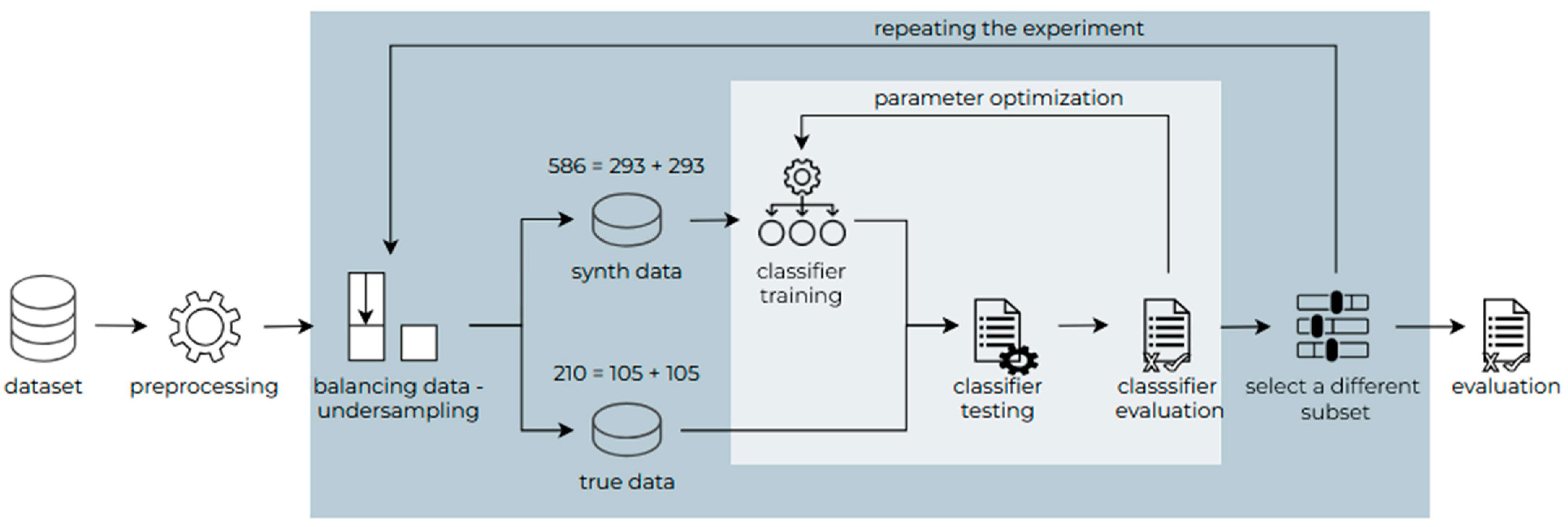
In the first case, the possibility of training the classifiers on synthetic data only and then testing them on real data only was investigated. The dataset was imbalanced—the LSTM class had twice as many synthetic records and three times as many real records as the SARIMA class; therefore, the data were balanced according to the class with fewer records—SARIMA. Random undersampling was applied for balancing.

Tree-Based Parzen Estimator was used to optimize the parameters of the MLP, random forest, and gradient boosted tree classifiers, while the hill climbing technique was applied to the remaining classifiers. To make the balancing less influential on the result, the whole process was repeated five times, and the average of the results was calculated. The flowchart of the research can be seen in Figure 4.

The results showed similar results as in the case of the not-augmented dataset, and even worse results, as the average accuracy was similar but the variation between class accuracy varied a lot. The random forest classifier achieved the best result—60.5%. The worst results were shown by Naïve Bayes, which failed to distinguish the class data at all and always guessed the LSTM class. It can be noted that all classifiers have learned to prioritize the LSTM class records. The results can be seen in

Table 7. Classifier evaluation (dataset balanced to the smallest class).

Classifiers	Average Acc.	Best Case Metrics
		Classes	Recall	Precision	F1	Parameters
k-NN	0.570	LSTM	0.771	0.558	0.648	k = 7
		SARIMA	0.390	0.630	0.482
SVM	0.561	LSTM	0.847	0.556	0.671	c = 87.027
		SARIMA	0.323	0.680	0.438
Naïve Bayes	0.500	LSTM	1.000	0.500	0.666	any value of the max no. of norm values
		SARIMA	0.000	0.000	0.000
MLP	0.592	LSTM	0.800	0.579	0.672	22 iter., 4 layers, 17 neurons
		SARIMA	0.419	0.676	0.517
PNN	0.556	LSTM	0.876	0.550	0.676	theta plus 0.920, theta minus 0.372
		SARIMA	0.285	0.697	0.405
random forest	0.605	LSTM	0.800	0.608	0.691	199 trees, 17 tree depth
		SARIMA	0.485	0.708	0.576
gradient boosted trees	0.575	LSTM	0.685	0.571	0.623	173 trees, 5 tree depth
		SARIMA	0.485	0.607	0.539

.

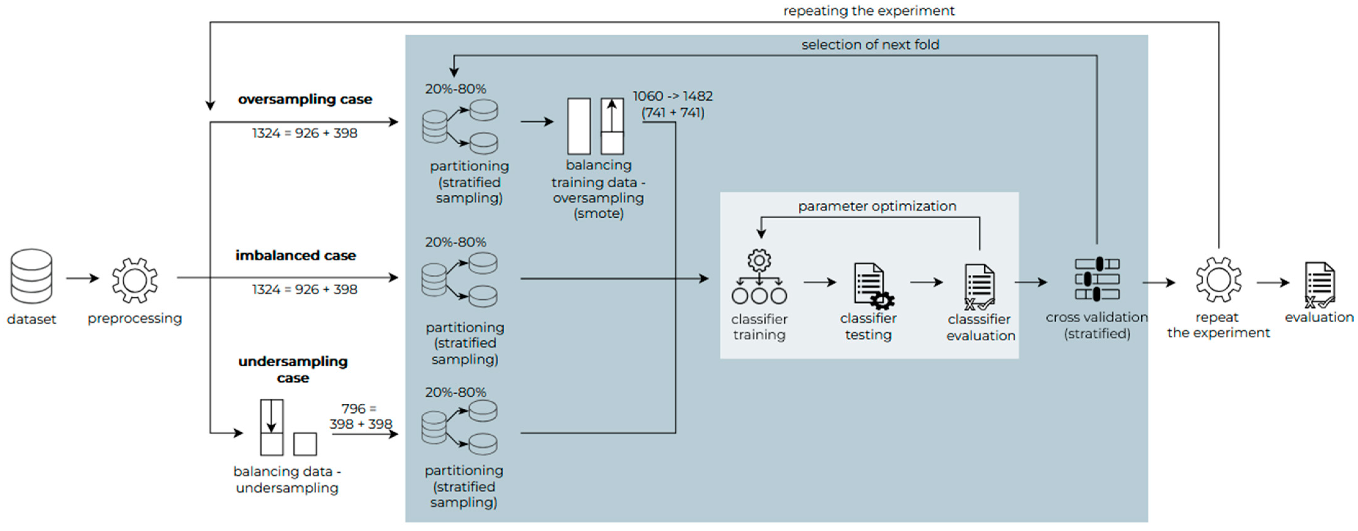
In the second case, to see how the accuracy of the classifiers changed, the classifiers were trained and tested on a real dataset augmented with synthetic data, i.e., the real dataset was merged with a synthetic dataset and the resulting dataset was submitted with a ratio of 80–20% for the training and testing of classifiers. The impact of balancing the dataset was simultaneously examined. The dataset was either unbalanced or balanced towards the SARIMA class with the fewest records (random undersampling) or balanced towards the LSTM class with the most records (oversampling using the Synthetic Minority Oversampling Technique (SMOTE)). For each data balancing case, cross validation with five subsets and stratified distribution was applied to validate the results. Finally, each experiment was repeated five times, and the average accuracy was evaluated.

All three cases of the real and synthetic data balancing strategies are illustrated in Figure 5. The balancing of the oversampled dataset was performed after the splitting of the dataset without affecting the testing of the data and thus distorting the results. In the case of an undersampled dataset, the balancing of the dataset was performed before the cross validation with the same options.

Analyzing the results between the sampling techniques, the imbalanced and oversampled options provided the highest average accuracy; however, they also showed the biggest variations between each class’s accuracy (see

Table 8. Accuracy and best model parameters for forecasting method prediction for different sampling techniques in mixed real and synthetically augmented datasets.

	Classifiers	Average Acc.	Best Case Metrics
			Classes	Recall	Precision	F1	Parameters
Oversampled	k-NN	0.705	LSTM	0.714	0.840	0.772	k = 9, knn smote = 44
			SARIMA	0.683	0.507	0.582
	SVM	0.745	LSTM	0.984	0.722	0.834	c = 0.049, knn smote 50
			SARIMA	0.188	0.796	0.205
	Naïve Bayes	0.708	LSTM	0.998	0.705	0.827	85 max number norm. val., knn smote 36
			SARIMA	0.030	0.923	0.058
	MLP	0.744	LSTM	0.768	0.852	0.808	143 iter., 5 layers, 40 neurons, knn smote 5
			SARIMA	0.690	0.562	0.620
	PNN	0.772	LSTM	0.890	0.802	0.844	theta plus 0.817, theta minus 0.362, knn smote 24
			SARIMA	0.489	0.658	0.561
	random forest	0.758	LSTM	0.836	0.836	0.835	28 trees, 6 tree depth, knn smote 27
			SARIMA	0.617	0.620	0.619
	gradient boosted trees	0.761	LSTM	0.852	0.827	0.839	82 trees, 5 tree depth, knn smote 10
			SARIMA	0.585	0.629	0.606
Imbalanced	k-NN	0.762	LSTM	0.876	0.800	0.836	k = 5
			SARIMA	0.489	0.631	0.551
	SVM	0.765	LSTM	0.887	0.798	0.840	c = 19.982
			SARIMA	0.479	0.647	0.551
	Naïve Bayes	0.706	LSTM	0.998	0.704	0.826	62 max number norm. val.
			SARIMA	0.025	0.909	0.048
	MLP	0.783	LSTM	0.893	0.812	0.850	171 iter., 4 layers, 48 neurons
			SARIMA	0.520	0.676	0.588
	PNN	0.777	LSTM	0.948	0.779	0.855	theta plus 0.661, theta minus 0.107
			SARIMA	0.374	0.756	0.500
	random forest	0.785	LSTM	0.914	0.807	0.857	139 trees, 27 tree depth
			SARIMA	0.492	0.712	0.582
	gradient boosted trees	0.769	LSTM	0.888	0.802	0.843	54 trees, 6 tree depth
			SARIMA	0.489	0.654	0.560
Undersampled	k-NN	0.683	LSTM	0.701	0.704	0.702	k = 9
			SARIMA	0.706	0.702	0.704
	SVM	0.642	LSTM	0.685	0.653	0.669	c = 57.519
			SARIMA	0.635	0.669	0.652
	Naïve Bayes	0.513	LSTM	0.997	0.511	0.676	65 max number norm. val.
			SARIMA	0.047	0.950	0.090
	MLP	0.731	LSTM	0.741	0.735	0.738	95 iter., 1 layer, 67 neurons
			SARIMA	0.733	0.739	0.736
	PNN	0.704	LSTM	0.773	0.704	0.737	theta plus 0.427, theta minus 0.138
			SARIMA	0.675	0.749	0.710
	random forest	0.740	LSTM	0.776	0.733	0.754	187 trees, 22 tree depth
			SARIMA	0.718	0.762	0.739
	gradient boosted trees	0.717	LSTM	0.711	0.736	0.723	21 trees, 6 tree depth
			SARIMA	0.746	0.720	0.733

). Meanwhile, the undersampled option led to well-balanced accuracy between both classes in most cases, while the accuracy of the models increased by almost 10% in comparison to the real dataset only.

After multiple testing cases, the MLP classifier with the undersampled dataset and the parameters set to 95 iterations, one layer, 67 neurons, the “relu” activation function, and the “adam” solver should be used to achieve the highest and more balanced prediction of both classes. In Figure 6, a case where the average accuracy is 70% (71% for LSTM and 69% for SARIMA) is illustrated (see Figure 6a). The analysis of the real (b) and synthetic (c) data among this case illustrates that the classification accuracy is a little bit higher for the real data (72%) rather than the synthetic (69%).

5. Discussion

This research concentrated on the prediction of the best time series forecasting data method. As a test case, multiple companies’ accounting data were selected and aggregated by month to predict the next 12-month potential purchase costs for each partner. This allowed us to form a dataset where 21 statistical time series measures were used as features for the best forecasting model definition.

The initial experiments (presented in chapter three) illustrated the need for a choice between more accurate average accuracy and a balance between each class prediction accuracy. This was affected by the imbalanced dataset and the limited number of records in the dataset. For example, the highest average accuracy was achieved using an imbalanced dataset and a random forest method—78.5%. In this case, the recall for the LSTM method was 91% and for SARIMA was 49%. This did not seem fair and should not have been accepted as a trusted model. Meanwhile, for the undersampled dataset, the highest accuracy was achieved by random forest and reached only 74% on average, but both classes had a very similar recall.

The Naïve Bayes method was probably the worst model in terms of the balance between classes. In all cases, it had the lowest average accuracy as well as always preferring one class (LSTM) against the second one (SARIMA). This could be explained by the nature of the probabilistic model and the variety of the features and results, where the Naïve Bayes method did not wave enough cases to match all possible cases for both classes.

This could be explained by the fact that random forest is better for matching to complex feature interactions, the prioritization of the features, weighted voting, and adjusting class weights to balance the classes, dynamically ignoring irrelevant features. Naïve Bayes does not have these features and treats all features as equally relevant and also does not work in this case, as all the features in this dataset are continuous and do not necessarily match Gaussian distribution.

A clear difference between the used classification models (except Naïve Bayes) was not very visible—some models worked better in one situation, some in another. This did not allow us to estimate what had the biggest effect on the average classification accuracy, as multiple factors might have affected it: a non-linear, complex dependency between features; a class imbalance or lack of feature value diversification for certain classes; and a limited number of records in the dataset. Random forest usually shows the best accuracy, because it is able to balance all of the properties, despite not being the fastest one.

While undersampling helps to balance the class accuracy, an attempt to increase the accuracy by generating synthetic data was performed (presented in Section 4). Different time series generation strategies were applied to generate more data for forecasting using different methods. By augmenting the dataset with the synthetically generated time series data, the dataset increased from 424 to 1324 records, adding 900 based on synthetic data. The purpose of the synthetic data was to add some time series with different patterns, as the real accounting data had a high level of variation and a lack of seasonality.

The ideal situation would be if we could train the model with synthetic data and accurately predict the best forecasting method for real data. This approach was tested (Chapter 4.4) and indicated that it did not provide good results—the average accuracy was close to 55%, but it was not balanced between each class, even if the dataset was undersampled. Such results might have been affected by the fact that real data did not match the patterns reflected in the synthetic dataset. However, to specify the specific patterns and reflect them, synthetic data were not an option, as they would require additional resources, while the purpose of the automated forecasting method selection was mainly to reduce the forecasting process resource usage.

Mixing real and synthetic data for training and testing was an option, as it would increase the dataset size and reflect patterns from both the real and synthetic time series. This approach for dataset balancing using oversampling with SMOTE was tested, with undersampling to the smaller class and usage of the imbalanced cases also tested. The same tendency was noticed as with real data only—undersampling in this case worked better than other strategies in the case of average accuracy and a balance between the accuracy of each class. The increase in dataset size through synthetic data generation contributed to an improvement in forecasting method selection. In comparison to real undersampled datasets, the average accuracy for real + synthetic dataset usage increased by approximately 8%. This was a statistically significant difference (using t-test for the seven cases, p = 0.0444).

All the results indicated that the synthetic time series generation for forecasting method selection had potential for increasing the accuracy. In this study, only several different patterns of synthetic data were generated and were allowed to generate twice as much data as we had in the real dataset. Generating a wider range of patterns and a higher volume of variations for each of them could lead to even higher accuracy. The increase in classification accuracy might have been affected by the increase in the training set as well as the introduction of more patterns in the time series. The fact that oversampled data did not perform much better than imbalanced data, but were a bit better than the undersampled dataset models, gave us reason to believe the variety of different patterns introduced was more important than the increase in the training dataset. The tested classification model’s accuracy varied for the analyzed cases, as they were different in their nature, bias variance, complexity, hyperparameter sensitivity, etc. As the accounting data were diverse, the classification model selection was also very dependent on the data. Therefore, modelling different datasets and model variations gave us new knowledge towards the search for the most suitable AutoML solution for financial accounting time series preprocessing and prediction.

This research was performed on company accounting data, aggregating the data for each month. The data normalization and the statistical measurement used as features for model prediction reduced the chance that the same approach would not work for another data aggregation period; however, it was not tested in this research and should be considered. Despite this, the research results indicated their potential to be applied in cases where a high volume of time series exist and it is not realistic to work on them manually, while the forecasting results could lead to better performance or planning. The company management case is the most common example—if a company wants to predict the different metrics (orders, purchases, debts, complains, costs, etc.) of its collaboration with all of its clients (for which the numbers can reach hundreds or even thousands of clients), automation is necessary. Proper forecasting of different metrics could be used as a tool for decision support or even undesired case prevention by applying some automated actions in advance, such as automatically estimating the potential best time series data forecasting method whose performance is 74% better than using a random one or modelling all possible cases (which could lead to high resource consumption). Based on the prediction, the time series forecasting count can be performed automatically too and leads to further steps oriented on notifications and even certain decision-making actions.

6. Conclusions and Future Work

Training time series data forecasting method selection models only on synthetic data is not a suitable option for selecting the best model for forecasting time series data. The experiments illustrate that fully synthetic data usage for training model for testing with real data cannot increase the model accuracy, and even decreases accuracy by almost 20%, even if the number of records increases multiple times. The need for real data is a must in the scope of the analyzed case.

The undersampling strategy for dataset balancing is the best option for forecasting the method prediction accuracy. Undersampling showed the best results for all our experiments with accounting data for time series model prediction: real data were used for model training and testing; synthetic data for training and real data for testing; and a mix of real and synthetic data for both training and testing. This indicates the importance of class balance and the limitations of data augmentation methods for training datasets.

The combination of real and synthetic data can improve the accuracy of the classifier. The experiment results indicate that the change is statistically significant (p < 0.05), which proves the potential of synthetic data generation for the best time series model prediction.

Data augmentation for the best time series forecasting model selection should take into account both synthetic data generation and undersampling to balance the data and guarantee that class prioritization will be avoided. Experiments with data sampling strategies show that the highest average accuracy can be achieved with an imbalanced dataset, but the accuracy of the classes becomes unbalanced as well. While undersampling reduces the average accuracy, it also guarantees both classes will be equally reflected in the model.

Synthetic time series generation to extend a dataset for best time series data forecasting model selection is an effective way to increase the model accuracy. The experiment results illustrate that it is possible to achieve up to 74% of the accuracy and maintain the balance between classes in comparison to a not-augmented dataset, where the maximum accuracy reached 65% only. In some cases, this might be enough, while other areas would require a higher accuracy. Considering the limited number of data augmentation patterns, the generation of synthetic data seems very promising and leads to a hope that the accuracy could be increased even more by extending the dataset with new data records.

For higher applicability, further research could concentrate not only on the forecast method prediction, but the best parameter estimation as well. Different strategies should be tested to estimate how effective the model and its parameter prediction is in comparison to the AutoML approach, including the forecasting error and resource utilization.