Singularity Analysis and Mode-Switching Planning of a Symmetrical Multi-Arm Robot

Abstract

Inspired by changing the operation mode via branch-chain switching, a symmetrical multi-arm robot is proposed to meet the demand of continuous high-performance output. The kinematics and Jacobian matrix of the mechanism are established and solved, and the parameter expression when singularity occurs is obtained. As Type-I singularity is the key limiting factor of continuous motion, a branch-chain switching and motion planning method is proposed. Numerical simulation and joint interpolation control are explained according to the pseudo-inverse matrix. The mechanism completes the switching between the executing branch chain and the branch chain to be executed to realize continuous rotation with a large angle. The results prove the feasibility of the design and the correctness of the model, proving that this method can be a reference method for the design of this kind of robot.

1. Introduction

With the rapid development of robot technology, robots have evolved from having a single operation mode to multi-function integration and fusion modes. They often need high working reliability and mode reconstruction to meet and adapt to the requirements of multi-tasking with high performance. Compared with single-arm robots, the multi-arm structure has more flexible operability and stability and can complete relatively complex tasks [1,2,3,4]. Many space on-orbit robots, such as Dextre [5] and Robonaut [6], are equipped with two mechanical arms, and each mechanical arm has seven degrees of freedom (DOFs). Ranger [7], a multi-arm space robot developed by Maryland University, is equipped with hands at the end of its mechanical arms to realize various grasping tasks.

When the configuration of a robot is determined, the tasks it can perform can only be operated according to the configuration structure. In order to realize the diversified manipulation of robots, researchers have proposed a multi-arm robot with structural reconfiguration characteristics. Typical designs of reconfigurable space multi-arm robots include the following: The reconfigurable space mechanical arm proposed by Nobumas [8] has five rotary joints, two of which can be connected autonomously. The hand and end effector of the mechanical arm are standardized parts, and the hand can enter the actuator and connect with it to realize the reconfiguration of the mechanical arm. The RBR robot proposed by Hiroshi [9] is another representative reconfigurable space mechanical arm. It can realize a three-arm mode and change the other two modes according to different tasks. One is the standing mode, where each mechanical arm and the base hub are released and then converted into the operation mode. The other mode involves one mechanical arm being in a standing state, while the other two arms are connected to form an operating state. Aghili [10] and others designed a reconfigurable space robot that can reconfigure itself from using one arm to using both arms by locking joints. Ibarreche [11] proposed a six-DOF reconfigurable parallel manipulator that has various motion modes, enabling it to adapt to different tasks.

When a multi-arm robot is operating, it encounters an inevitable singularity that severely limits its range of motion and performance. Through the connection and release of different branches and operating objects, the operation mode and then the operation performance can be changed. Researchers regard the whole system of a multi-arm robot and its operating objects as the topological form of a parallel mechanism, and they have carried out research on configuration design and mode-switching planning for multi-arm robots. Corves [12] proposed a multi-mechanical arm robot with structure and performance reconfiguration based on the design idea of a parallel mechanism that can realize the repetitive grasping of operative targets and mechanical performance reconfigurations. Tian [13,14,15,16] proposed a design of a multi-fingered grasping robot; the researcher compares the performance indexes of the obtained mechanism by combining the operating target with the operating branch chain and finally designs an ideal robot. According to the similarities and differences between mechanical arm robots and multi-fingered arm parallel robots, Ebert [17] analyzed the realization requirements and methods of grasping and operating under different driving types based on the angle of the parallel mechanism, combined with the mechanism constraints and the characteristics required to grasp objects. Jin [18,19] and others synthesized a multi-arm mechanism with a large rotary angle using Lie theory regarding the composition of different branches and operating objects as the topological form of the parallel mechanism. The designed mechanism has the high-performance characteristics of continuous large-rotary-angle output. Zhao [20] designed a kind of multi-arm robot with different modes via branch-chain switching and represented its motion form with a motion set method. Integrating multiple parallel mechanisms into a multi-fingered dexterous hand can significantly enhance a robot’s in-hand manipulation performance [21]. Xue [22] proposed a configuration optimization method for a dual-arm reconfigurable space robot based on closed-chain inertia matching, which allows for selecting a configuration with better performance during the task execution process. Moosavian [23] proposed a new method for the static enhancement of manipulators using lockable passive joints, resulting in a manipulator with high stiffness and the advantage of effectively avoiding singular configurations.

A symmetrical multi-arm robot is proposed that has four branches with the same structure, and three of them perform operation tasks. When the mechanism moves to near singularity, the fourth branch chain unfolds and connects with the operating object, while the branches near singularity are released with the operating objects. Due to the symmetrical structure of the branch chains, the mechanism can continue to perform the same operation tasks after switching, which ensures a continuous high-performance output. The structure of this paper is as follows: In Section 2, a symmetrical multi-arm robot is proposed, the kinematics model of the mechanism is established, and the velocity Jacobian matrix is solved. In addition, the singularity is analyzed, and the typical configuration diagrams of different singularity types are introduced. In Section 3, the motion planning of branch-chain switching is carried out by avoiding Type-I singularity, and the corresponding mode-switching control model and path planning algorithm are verified by simulation.

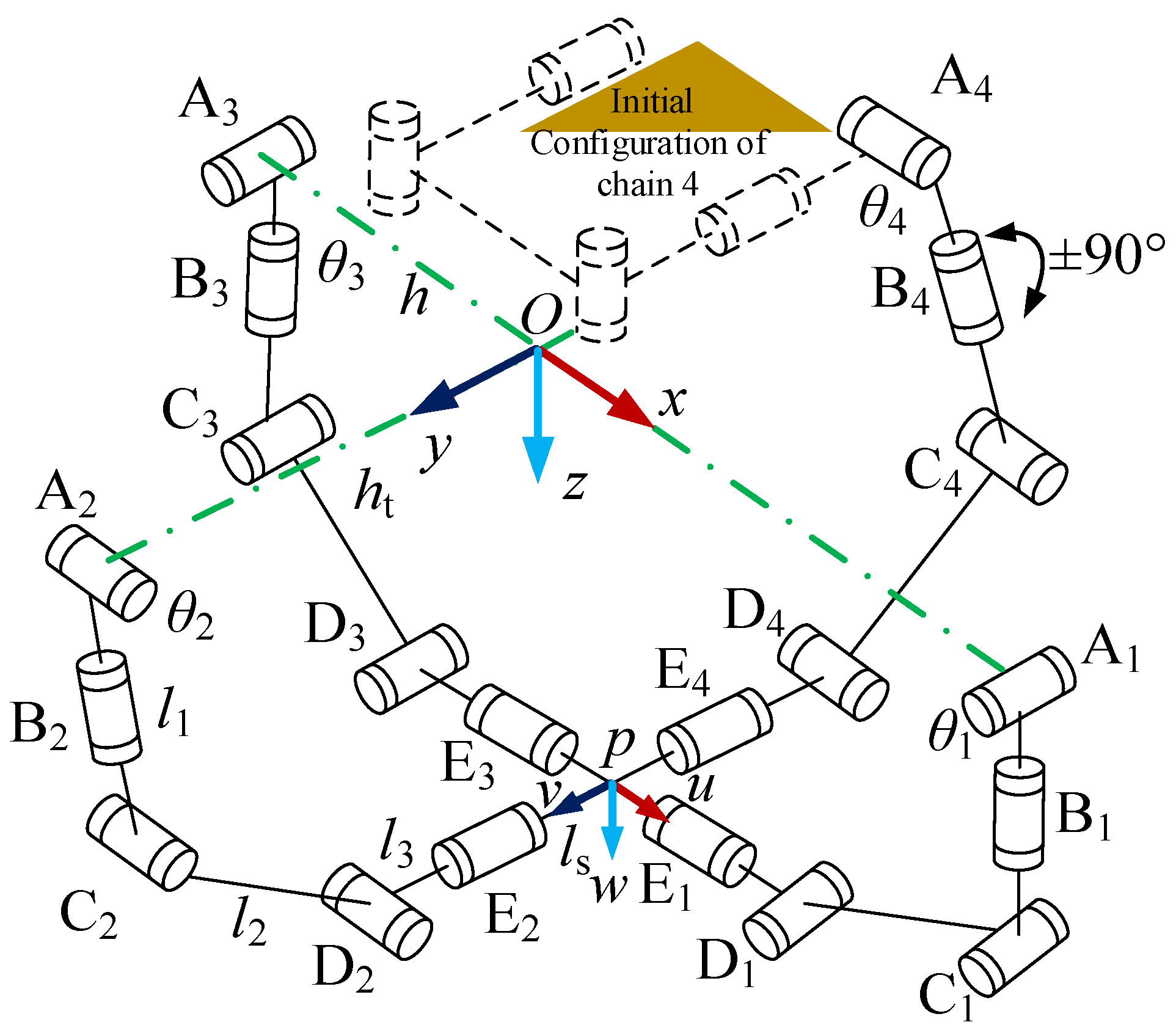
2. Mechanism Design and Analysis of a Multi-Arm Robot with a Symmetrical Structure

A system consisting of a multi-arm robot and an operating object can be regarded as the topological form of a parallel mechanism. The advantage lies in that the topological form and working performance of the formed parallel mechanism can be changed by the connection and release of different branches and operating objects to change the operation mode. In mechanism design, a large rotary angle and high stiffness have always been the design goals for high performance; however, large-rotary-angle motion is often limited by the occurrence of singularity. In this section, a multi-arm robot is designed to realize 2R1T bidirectional large-rotary-angle operation, and the mode switching of the mechanism is studied.

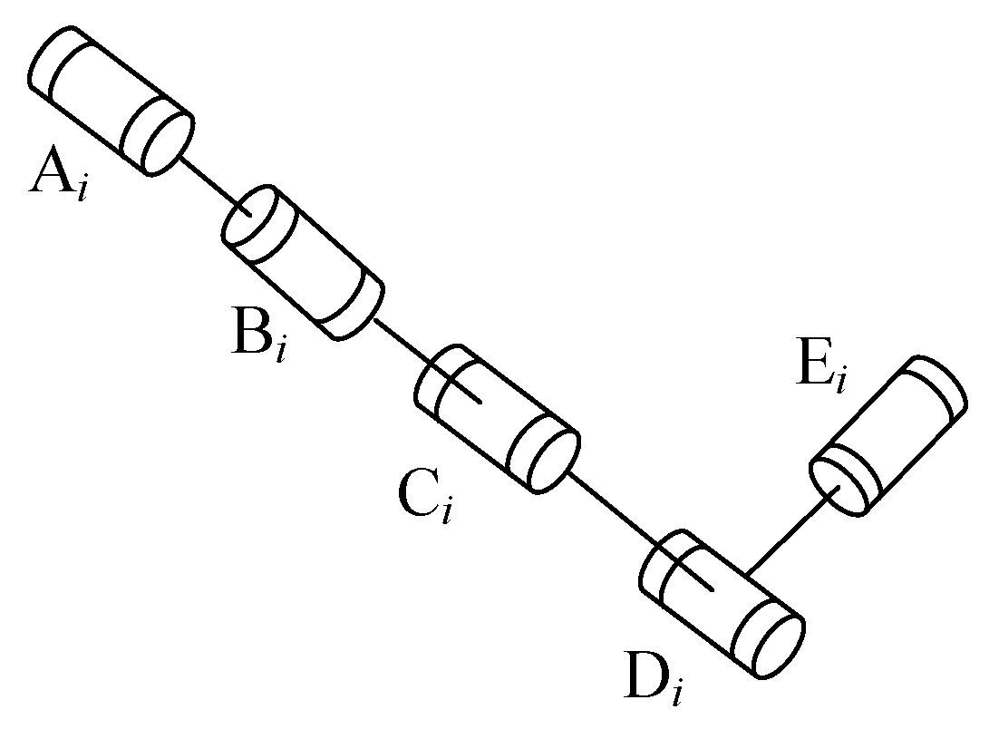
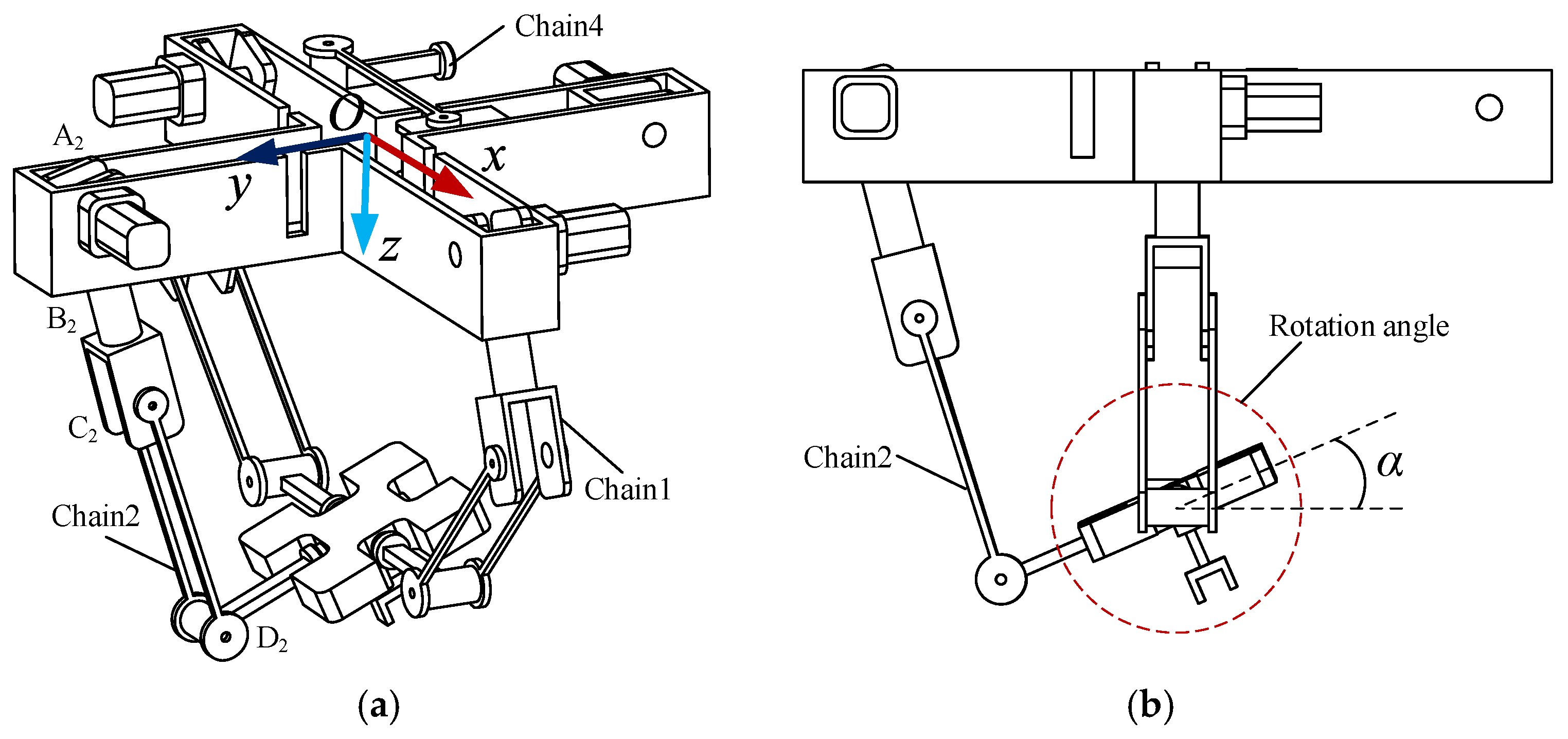
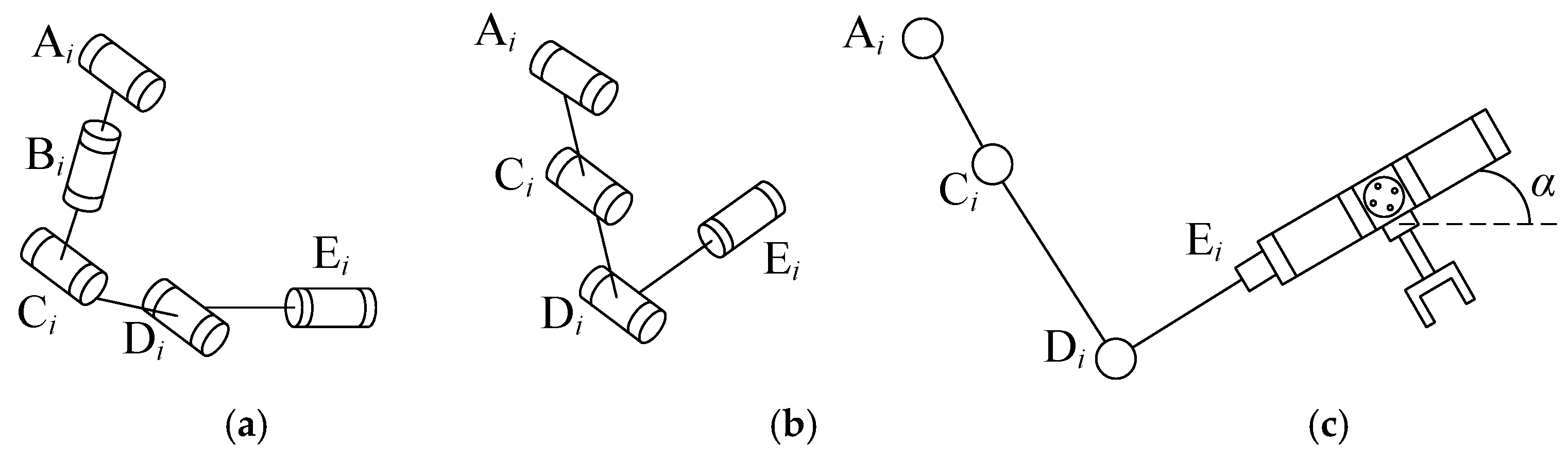
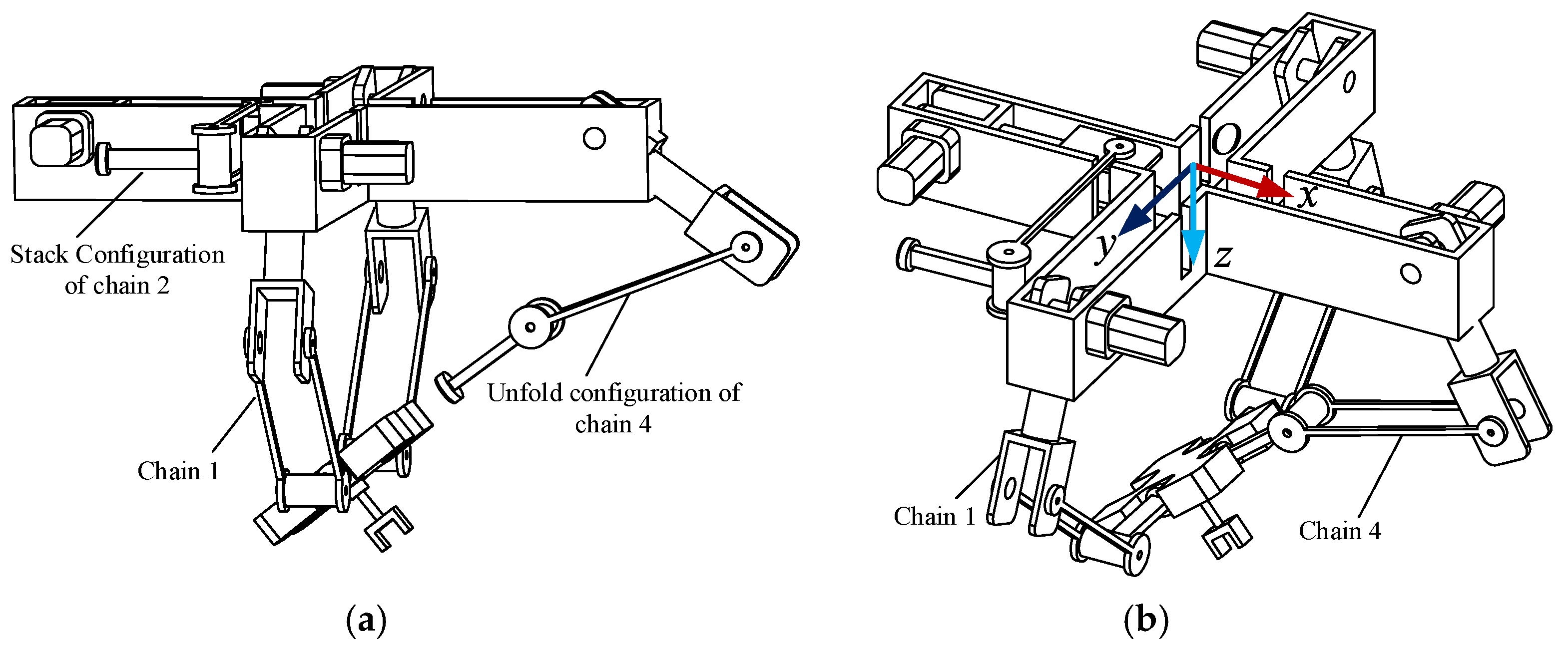
2.1. Mechanism Design

Firstly, it is assumed that the mechanism can complete rotary operations around the x- and y-axes and movement operations along the z-axis for the operating object. Its operation mode can be expressed using the motion set method [24,25] as M = (0 0 T_z; R_x R_y 0). Therefore, the intersection of the end motion forms of each branch chain should be M, where $\mathrm{M}={\mathrm{S}}_{i-1}\cap {\mathrm{S}}_i\cap {\mathrm{S}}_{i+1}$, (i = 1, 2, 3). T_z represents the moving platform’s movement along the z-axis, and R_n (n = x, y) represents the moving platform’s rotation around the n-axis.

The selected motion form to construct a multi-arm robot is S = (T_x 0 T_z; R_x R_y 0). In a four-chain symmetrically arranged robot, the branch chain has two forms of motion: (T_x 0 T_z; R_x R_y 0) and (0 T_y T_z; R_x R_y 0). When the branch chain is connected to the operating object, the motion form of the operating object is the intersection of the two motion forms of the branch chain; that is, M = (0 0 T_z; R_x R_y 0).

Figure 1 shows a symmetrical multi-arm robot, and the branch-chain structure is R^xR^xR^xR^y, where R^x and R^y indicate that, after the branch chain is connected to the operating object, the axis of the rotary pair is parallel to the x-axis and y-axis, respectively, and the second joint is a folding joint, which can stack the branch chain in the plane storage area through self-rotation. When any three branches or all branches are connected to an object, the branch chain completes the set M = (0 0 T_z; R_x R_y 0).

Figure 1 is a schematic diagram of different operation modes of a structurally symmetrical multi-arm robot. The two working modes are as follows: (a) any three branches are connected to the operating object to produce the 2R1T motion mode, and (b) four branches are connected to the operating object at the same time. In the first working mode, the mechanism can be connected to the operating object via different branches to realize the performance reconstruction and mode switching of the formed parallel mechanism, as shown in Figure 1a. In the second mode, the mechanism and the operating object can form an over-constrained parallel mechanism state. Although the rotary angle range is limited, it has better stiffness performance due to the existence of over-constrained characteristics, as shown in Figure 1b.

2.2. Kinematics Analysis

Figure 2 shows the kinematic model of the structure diagram of the structurally symmetrical multi-arm robot, which contains four identical branch chains. Each chain has five rotational joints, denoted by A_i, B_i, C_i, D_i, and E_i (i = 1, 2, 3, 4). θ_i is the angle between line A_iB_i and line OA_i, and it is the actuation angle of each chain. When the branch chains in the mechanism are connected to the object to form the topological form of the parallel mechanism, the object can be regarded as the moving platform in the parallel mechanism, and each branch chain can be regarded as the moving branch chains. According to the theory of parallel mechanisms, inverse kinematics analysis can be used to solve the variables of driving joints by providing the attitude and position of the terminal moving platform. In order to make the mechanism move according to 2R1T, joint B is locked when the joint moves to 90° after the branch chain is unfolded, and the branch chain of the parallel mechanism is R^xR^xR^xR^y.

Coordinate system O-xyz and coordinate system p-uvw are set on fixed and moving platforms, respectively. The motion form of the coordinate system {p} in {O} is p = (α, β, z)^T, where α represents the rotary angle around the x-axis and β is the rotary angle of the moving platform around the y-axis. Therefore, the transformation matrix R of the coordinate system {p} relative to {O} can be written as follows:

$$\mathit{R}={\mathit{R}}_x(\alpha ){\mathit{R}}_y(\beta )=\left[\begin{array}{ccc}1& 0& 0\\ 0& c\alpha & -s\alpha \\ 0& s\alpha & c\alpha \end{array}\right]\left[\begin{array}{ccc}c\beta & 0& s\beta \\ 0& 1& 0\\ -s\beta & 0& c\beta \end{array}\right]=\left[\begin{array}{ccc}c\beta & 0& s\beta \\ s\alpha s\beta & c\alpha & -s\alpha c\beta \\ -c\alpha s\beta & s\alpha & c\alpha s\beta \end{array}\right]$$

(1)

where si represents sini, and ci represents cosi, where i = (α, β).

For the convenience of calculation and expression, each rod length parameter is defined by the following vectors:

$${\mathit{a}}_i=‖O{A}_i‖, {\mathit{b}}_i=‖A_i{C}_i‖, {\mathit{c}}_i=‖C_i{D}_i‖, {\mathit{d}}_i=‖D_i{E}_i‖, {\mathit{e}}_i=‖p{E}_i‖$$

The coordinates of point Ai in the coordinate system {O} are a₁ = (h,0,0)^T, a₂ = (0,h,0)^T, a₃ = (−h,0,0)^T, and a₄ = (0,−h,0)^T.

The coordinate of the point C_i in the coordinate system {O} is

c_i =a_i+ ((cos(i − 1)π/2)l₁cosθ_i, (sin(i − 1)π/2)l₁cosθ_i, l₁sinθ_i)^T, i = 1–4.

The coordinate of point E_i in the coordinate system {O} is

e₁ = R^be₁ + o e₂ = R^be₂ + o e₃ = R^be₃ + o e₄ = R^be₃ + o

where ^be₁ represents the coordinate vector of E_i in the {p} coordinate system and o = (0,0,z)^T.

The coordinate of point D_i in the coordinate system {O} is d_i=R(^bd_i + ^be_i) + o, where i = 1–4.

According to the C_iD_i geometric constraint of rod length, the coordinate vectors of C_i and D_i satisfy the following equation:

(c_i − d_i)^T (c_i − d_i) = ||C_iD_i||

(2)

Equation (2) expresses the geometric operation relationship between joint angle θ_i and α, β, z, and the rod length parameters of the mechanism. As described in the preceding section, a rotary motion is achieved by the mechanism about the x-axis, a rotary motion about the y-axis, and a movement along the z-axis. When the mechanism is connected to the operating object, the number of independent drives required by the mechanism is 3. According to the traditional design method of parallel mechanisms, the first rotary pair closest to the fixed platform in each branch chain is selected as the driving joint in each branch chain, and the other joints are passive joints; this produces the 2R1T operation mode of the mechanism for operating objects.

$\mathbf{x}={[\alpha ,\beta ,z]}^{\mathrm{T}}$ and $\mathbf{q}={[{\theta }_1,{\theta }_2,{\theta }_3,{\theta }_4]}^{\mathrm{T}}$ represent the position and orientation matrix of the operating object and the angle matrix of the driving joint, respectively. After differentiating the time on both sides of Equation (2), the equation form ${\mathbf{J}}_{\mathrm{x}}\dot{\mathbf{x}}={\mathbf{J}}_{\mathbf{q}}\dot{\mathbf{q}}$ can be derived.

The matrix J_x and the matrix J_q can be obtained as follows:

$${\mathbf{J}}_{\mathbf{x}}={\left[\begin{array}{ccc}{a}_{11}& a_{12}& a_{13}\\ a_{21}& a_{22}& a_{23}\\ a_{31}& a_{32}& a_{33}\\ a_{41}& a_{42}& a_{43}\end{array}\right]}_{4\times 3},{\mathbf{J}}_{\mathbf{q}}=\left(\begin{array}{ccc}{u}_1& \cdots & 0\\ ⋮& \ddots & ⋮\\ 0& \cdots & u_4\end{array}\right)$$

(3)

Therefore, the total Jacobian matrix J of the mechanism can be written as follows:

$$\mathbf{J}={\mathbf{J}}_{\mathrm{x}}^{-1}{\mathbf{J}}_{\mathbf{q}}$$

(4)

where a_ij and u_i are the functions of the motion parameters α, β, z, and θ_i and the length of the rod.

The kinematics and Jacobian matrix of the parallel mechanism can be obtained by the above analysis when the four branches of the mechanism are connected to the operating object. The kinematics and Jacobian matrix can be obtained according to the corresponding situation of different branches when the parallel mechanism is composed of three branches and the operating object. Taking the mechanism composed of branch chains 1 to 3 as an example, the matrices J_x1 and J_q1 in Equation (4) become 3 × 3 matrices, and the corresponding equation relationship can be expressed as follows:

$$\left(\begin{array}{ccc}{u}_1& 0& 0\\ 0& u_2& 0\\ 0& 0& u_3\end{array}\right)\left(\begin{array}{c}{\dot{\theta }}_1\\ {\dot{\theta }}_2\\ {\dot{\theta }}_3\end{array}\right)+\left(\begin{array}{ccc}{a}_{11}& a_{12}& a_{13}\\ a_{21}& a_{22}& a_{23}\\ a_{31}& a_{32}& a_{33}\end{array}\right)\left(\begin{array}{c}\dot{\alpha }\\ \dot{\beta }\\ \dot{z}\end{array}\right)=0$$

(5)

The coefficient matrices J_x1 and J_q1 in the above equation are the basis for judging the singularity of the mechanism.

By further differentiating Equation (5), we obtain

$$\left(\begin{array}{c}{\dot{\theta }}_1\\ {\dot{\theta }}_2\\ {\dot{\theta }}_3\end{array}\right)=-{\left(\begin{array}{ccc}{u}_1& 0& 0\\ 0& u_2& 0\\ 0& 0& u_3\end{array}\right)}^{-1}\left(\begin{array}{ccc}{a}_{11}& a_{12}& a_{13}\\ a_{21}& a_{22}& a_{23}\\ a_{31}& a_{32}& a_{33}\end{array}\right)\left(\begin{array}{c}\dot{\alpha }\\ \dot{\beta }\\ \dot{z}\end{array}\right)$$

(6)

The Jacobian matrix ${\mathbf{J}}_1=-{\mathbf{J}}_{\mathbf{x}1}^{-1}{\mathbf{J}}_{\mathbf{q}1}$ under this configuration can be obtained.

Similarly, when the mechanism is connected to the operating object through any three branches, the mechanism also has the relational equations of the other three groups of Jacobian matrices; that is, the motion correspondence between the driving input values of the branches connected to the operating object and the output motion values of the operating object and the Jacobian matrices corresponding to these motion relations can be obtained using the same method.

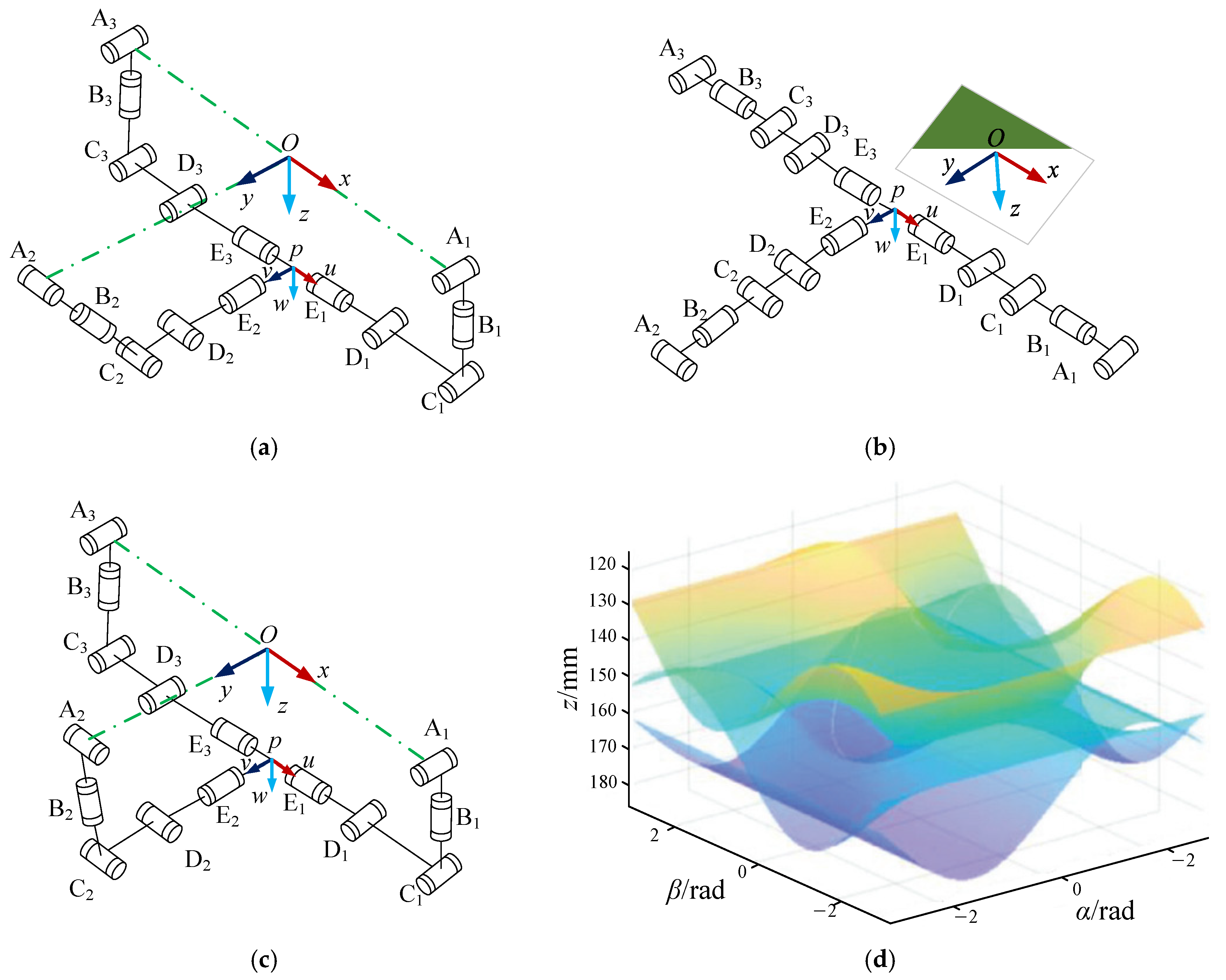
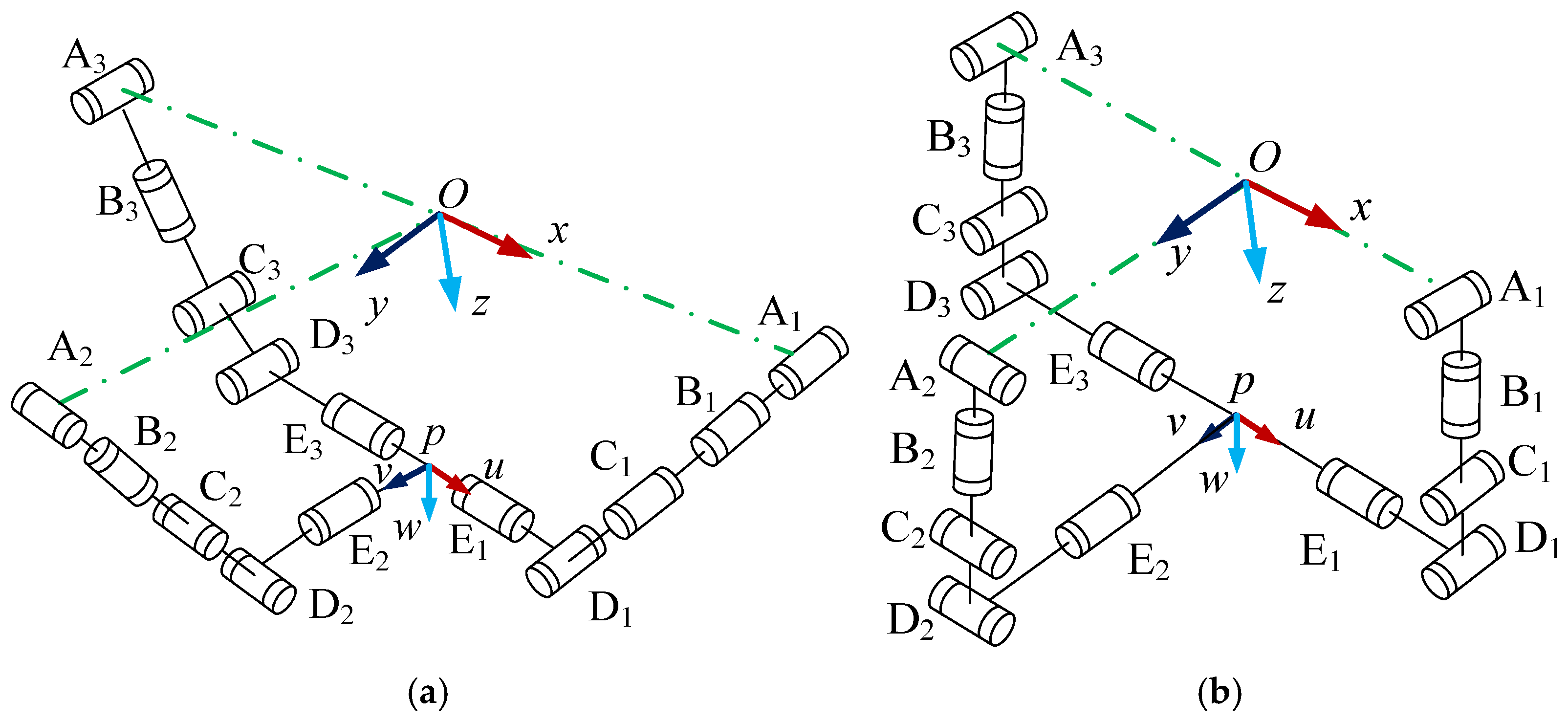
2.3. Singularity Analysis of Mechanism

When a singularity occurs in the mechanism, the configuration of the parallel mechanism can be reconstructed by switching the branch chain of the multi-arm robot to connect with the operating object, thus realizing the continuous and high-performance operation of the operating object. This section analyzes the singularity of the parallel mechanism composed of the mechanism and the operating object, and it studies the work planning and implementation of the mechanism mode switching and continuous operation by taking the example of avoiding singularity. The singularity of the parallel mechanism can be divided into three types: inverse kinematics singularity, forward kinematics singularity, and combined singularity [26].

2.3.1. Forward Kinematics Singularity

Due to the symmetry of the mechanism, this study analyzes the singularity of the configuration of the parallel mechanism composed of three branches of the mechanism, and when J_x1 deteriorates, it produces forward kinematic singularity. According to Figure 2, J_x1 in Equation (5) can be rewritten as follows:

$${\mathbf{J}}_{\mathbf{x}1}={\left[\begin{array}{ccc}{x}_{L1}& z_{L1}& 0\\ x_{L2}& z_{L2}& h_{\mathrm{t}}c{\theta }_2{z}_{L2}-h_{\mathrm{t}}s{\theta }_2{x}_{L2}\\ x_{L3}& z_{L3}& h_{\mathrm{t}}c{\theta }_3{z}_{L3}-h_{\mathrm{t}}s{\theta }_3{x}_{L3}\end{array}\right]}_{3\times 3}$$

(7)

According to J_x1 defined in Equation (7), when θ₁, θ₂, or θ₃ is 90°, the elements of the row corresponding to the matrix are equal to zero, and the corresponding configuration of the mechanism is shown in Figure 3a. It can be seen from Equation (7) that, when the rotary angles α and β are zero at the same time and z is equal to zero, each behavior of the matrix J_x1 is zero, and its corresponding configuration is shown in Figure 3b.

Similarly, when any column in J_x1 is zero, the determinant |J_x1| becomes zero. By observing Equation (7), it can be seen that, when θ₁, θ₂, and θ₃ are 90° at the same time, the elements in the first column are zero, and their corresponding configuration is shown in Figure 3c. Secondly, when there is a linear correlation between rows or columns, the mechanism is also in a singularity. When members D₁E₁ and D₃E₃ are collinear and coplanar with members C₂D₂, the first column of the matrix J_x1 has a linear correlation with the third column. Due to the symmetry of the mechanism, the singularity of the branch chain is the same as that of branch chain 2 in other modes.

The above results are obtained by observing Equation (7), but all the position information of singularity in the process of mechanism motion can be obtained with an analytical method. Figure 3d shows the value corresponding to the determinant |J_x1| = 0 that corresponds to the rotary angles α and β when the position z of the operating object is given. It can be observed from Figure 3 that the configurations correspond to three branch links that are coplanar with the moving platform. This results in uncontrolled DOFs and an uncertain motion in the following motion process.

2.3.2. Inverse Kinematic Singularity

When the determinant of J_q1 is |J_q1| = 0, the inverse kinematic singularity of the mechanism appears; that is, the rank of J_q1 is less than the whole DOF of the mechanism. As J_q1 is a diagonal matrix, when any one or more diagonal elements are zero, its determinant is zero. Similarly, when the operating object is operated by branch chain 1, branch chain 2, and branch chain 3, the expression corresponding to J_q1 can be written as follows:

$${\mathbf{J}}_{\mathbf{q}1}={\left(\begin{array}{ccc}{u}_1& 0& 0\\ 0& u_2& 0\\ 0& 0& u_3\end{array}\right)}_{3\times 3}$$

(8)

The diagonal elements in J_q1 are symmetrical with the mechanism structure. Therefore, the matrix element u1 corresponding to the singularity in the first branch chain is analyzed. It can be seen from Equation (8) that, when u₁ is equal to 0, the link A₂C₂ and the link C₂D₂ in the branch chain are straightened or folded collinearly, and the mechanism is in the inverse kinematic singularity at this time. The condition in which the other two diagonal elements of J_q1 are zero has a similar physical interpretation for the other two branches. Figure 4 shows an example of the configuration when three branches of the mechanism are simultaneously located in the inverse kinematic singularity.

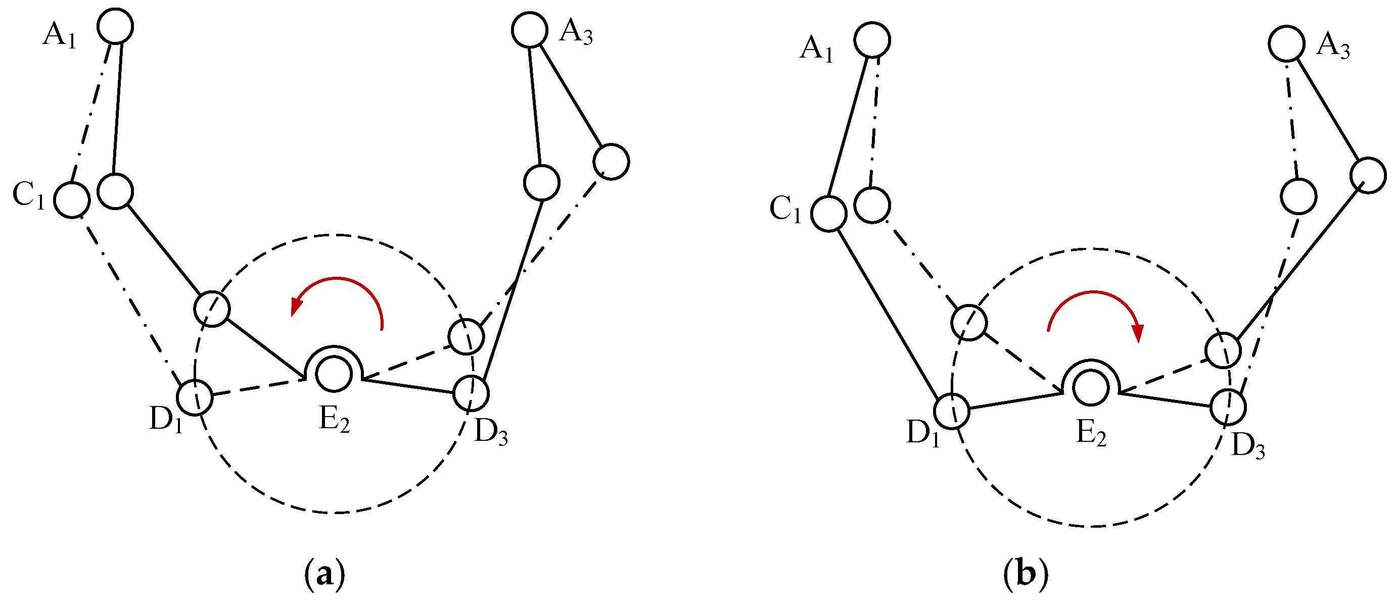
2.3.3. Combinatorial Singularity

When the rank of J_x1 and J_q1 is reduced, the mechanism produces a combined singularity in the process of motion, and this type of singularity is the combination of the above two singularities. From the above analysis, it can be seen that, if the lines related to D_iE_i are in the same plane position and A_iD_i are parallel to each other, and when either A_iC_i or C_iD_i are completely straightened or folded collinearly, the mechanism is in a combined singularity. Figure 3b and Figure 4b both show the combined singularity of the mechanism in three branches.

Several typical singularities of the mechanism are introduced. From the above results, it can be seen that, if the mechanism realizes the operation of a large rotary angle, the biggest limiting factor is the singularity of the branch chain, as shown in Figure 5. Figure 6 shows that the mechanism rotates the operating object through chain 1 and chain 3; when the mechanism moves to the inverse kinematics singularity, branch chain 4 is unfolded to connect with the operating object, and branch chain 2 is released from the connection with the operating object, so that the operating object can continue to rotate, thus realizing the large-rotary-angle operation.

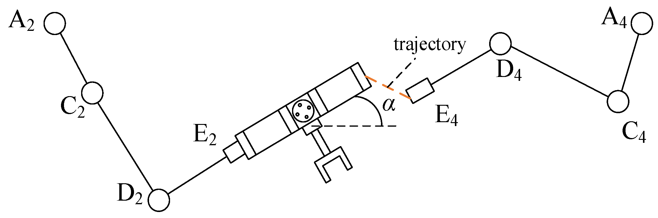
2.4. Motion Planning Based on a Type-I Singular Branch Chain

As mentioned in the previous section, the occurrence of the singularity of the branch chain is the biggest influencing factor for the mechanism to realize large-rotary-angle operation. Based on the mode-switching planning by releasing and connecting with the operating object through branch chain 2 and branch chain 4, respectively, it avoids the singularity of the branch chain. The whole process can be planned as follows:

(1) The occurrence of singularity for the mechanism

Figure 7 shows the movement of branch chain 2 in the mechanism for a singularity when the mechanism rotates about the x-axis. For the traditional parallel mechanism, the rotary angle has reached the motion limit. The configuration in Figure 7 corresponds to that in Figure 4a; that is, link A₂C₂ is collinearly straightened with rod C₂D₂. Therefore, the moving platform cannot continue to rotate in the same direction around the X-axis at this time. In the multi-arm robot, when branch chain 2 is singular or near a singularity, the opposite branch chain 4 can be unfolded and connected to the operating object to keep the continuity of motion. Branch chains 1 and 3 and branch chains 2 and 4 are opposite branches. When the members A_iC_i and C_iD_i are straightened and collinear, the branch chain is in Type I (inverse kinematic singularity), as shown in Figure 8.

(2) The opposite branch chain is connected to the operating object

In the second stage of the working process, when branch chain 2 moves to singularity, branch chain 4 unfolds and moves to the designated position and then connects with the operating object. Branch chain 2 and the operating object are folded in the designated area after being released, as shown in Figure 9. It can be divided into two motion processes. Branch chain 4 first moves to the position adjacent to the operating object, that is, position E₄, and keeps the slope of D₄E₄ the same as the slope of the operating object at the rotary angle α, as shown in the A_iC_iD_iE_i configuration in Figure 10. Then, point E₄ is positioned through each driving joint so that branch chain 4 is connected to the operating object.

(3) The maintenance of rotary continuity of the mechanism

As shown in Figure 11, when branch chain 4 is connected to the operating object, the topological form of the parallel mechanism at this time consists of branch chains 1, 3, and 4 and the operating object. The mechanism can be connected to the operating object through the three branch chains, and the operating object can continue to rotate around the x-axis. Figure 12 shows a structural diagram of the branch-chain switching and operating object. The rotary angle range of the operating object is mainly affected by the interference between the link A₄C₄D₄E₄ and the platform and the interference between the links in branch chain 4. In the next section, the planning and control of branch-chain folding and switching in the working process of the mechanism are discussed.

3. Simulation Control of the Planning of Branch-Chain Switching

3.1. Position and Pose Model of Branch-Chain Motion

Taking branch chain 4 as the branch to be executed as an example, its initial stacking position is planned from an unfolding to a docking position. In the movement process, branch chain 4 is an operation branch chain in a series. According to the D-H modeling method, the coordinate system of each joint is defined as shown in Figure 13. The flexion joint θ₂ rotates from 0° to 90° so that the plane A₄C₄D₄E₄ formed by the branch chain coincides with the plane Oyz and that the end of the branch chain is positioned based on the motion of θ₁, θ₃, and θ₄ and connected to the operating object.

When plane A₄C₄D₄E₄ coincides with plane Oyz, the driving joints in the operating branch chain are A₄, C₄, and D₄. The operating branch chain is equivalent to the planar 3R redundant DOF branch chain. Before the branch chain is docked with the operating object, the branch-chain end E₄ is moved to the designated position shown in Figure 13.

$$\left\{\begin{array}{c}{x}_{\mathrm{E}4}=x_p=0\\ y_{\mathrm{E}4}=y_p+\Delta y\\ z_{\mathrm{E}4}=z_p+\Delta z\end{array}\right.$$

(9)

According to the position condition in the figure, the following geometric constraints exist between the branch chain and the operating object: (a) the slope of the link D₂E₂ is the same as that of link D₄E₄, and (b) the angles between members D₄E₄ and C₄D₄ are greater than 90° and less than 180°.

$$\left\{\begin{array}{c}{k}_{D_2{E}_2}=k_{D_4{E}_4}\\ \cos <C_4{D}_4,D_4{E}_4>\in [-1,0]\end{array}\right.$$

(10)

According to the constraint conditions of Equations (9) and (10), the coordinate position of the point E₄ at the end of the branch chain is determined by giving the initial values of Δy and Δz. From the inverse solution of the parallel mechanism formed by branches 1, 2, and 3 and the operating object, the slope k_D2E2 of the link D₂E₂ can be obtained when the branches are switched; thus, the slope of the link D₄E₄ in branch chain 4 can be obtained.

3.2. Path Planning Algorithm for Branch Chains

The path planning of branch chain 4 from the initial position to the docking position is carried out. When the initial position Θ₀ and the termination state Θ_f of the joint in the branch chain are known, the problem of the branch-chain motion planning can be described by the motion of the joint planning.

$$\mathrm{\Theta }(t)=f(t)$$

(11)

The following condition needs to be met:

$$\mathrm{\Theta }(0)={\mathrm{\Theta }}_0,\mathrm{\Theta }(t_f)={\mathrm{\Theta }}_f$$

(12)

Based on the requirement of smoothness in the process of branch-chain motion, the boundary constraints of angular velocity are set as follows: $\dot{\mathrm{\Theta }}(0)=0$, $\mathrm{\Theta }(t_f)={\mathrm{\Theta }}_f$. Each joint function is expressed by a high-order polynomial:

$${\mathrm{\Theta }}_i(t)=a_{i3}{t}^3+a_{i2}{t}^2+a_{i1}t+a_{i0},i=1,2,\dots ,4$$

(13)

In order to avoid the singularity in calculation, the time t is unified.

$$\stackrel{⌢}{t}={\displaystyle \frac{t}{T}}$$

(14)

Here, T represents the movement time of the branch chain.

Each joint function can be written as follows:

$${\stackrel{⌢}{\mathrm{\Theta }}}_i(\stackrel{⌢}{t})={\stackrel{⌢}{a}}_{i3}{\stackrel{⌢}{t}}^3+{\stackrel{⌢}{a}}_{i2}{\stackrel{⌢}{t}}^2+{\stackrel{⌢}{a}}_{i1}\stackrel{⌢}{t}+{\stackrel{⌢}{a}}_{i0}$$

(15)

$${\dot{\stackrel{⌢}{\mathrm{\Theta }}}}_i(\stackrel{⌢}{t})=3{\stackrel{⌢}{a}}_{i3}{\stackrel{⌢}{t}}^2+2{\stackrel{⌢}{a}}_{i2}\stackrel{⌢}{t}+{\stackrel{⌢}{a}}_{i1}$$

(16)

After obtaining the parameters of Equation (15), the values of the actual joint angle and angular velocity can be obtained based on the joint angle and angular velocity obtained from the unified calculation. Based on the maximum value, the motion time of the branch chain can be obtained, and thus, the motion function of each joint can be obtained:

$${\mathrm{\Theta }}_i(t)={\stackrel{⌢}{\mathrm{\Theta }}}_i(\stackrel{⌢}{t}),{\dot{\mathrm{\Theta }}}_i(t)={\dot{\stackrel{⌢}{\mathrm{\Theta }}}}_i(\stackrel{⌢}{t})/T$$

(17)

The movement planning of the branch chain is carried out based on the pseudo-inverse matrix method [27]. The expected movement speed and angular speed of the branch-chain end can be planned through the error of the position and attitude of the branch-chain end relative to the expected state, as shown in Equation (18):

$$\left(\begin{array}{c}{v}_d\\ {\omega }_d\end{array}\right)=\mathit{K}\left(\begin{array}{c}{}^{0}r_i\\ \Delta {\Psi }_t\end{array}\right)$$

(18)

Here, v_d and ω_d represent the relative velocity and angular velocity of the end of the branch chain in the initial state, respectively; Ψ_t is the attitude deviation of the end of the branch chain relative to the end state; and r_E is the position vector of the target point relative to the end of the branch chain.

$${\mathit{r}}_E={\mathit{r}}_r-{\mathit{r}}_e$$

(19)

Here, r_r represents the position coordinate vector of the target point in the fixed coordinate system, and r_e is the coordinate vector of the end of the branch chain.

The angular velocity of each driving joint is calculated using the pseudo-inverse matrix method:

$$\dot{\mathrm{\Theta }}={\mathbf{J}}^{\mathrm{T}}{(\mathbf{J}{\mathbf{J}}^{\mathrm{T}})}^{-1}\left(\begin{array}{c}{v}_d\\ {\omega }_d\end{array}\right)$$

(20)

According to the constraint condition of the maximum angular velocity value, Θ is adjusted to make the planning result fulfill the requirements of the branch-chain motion.

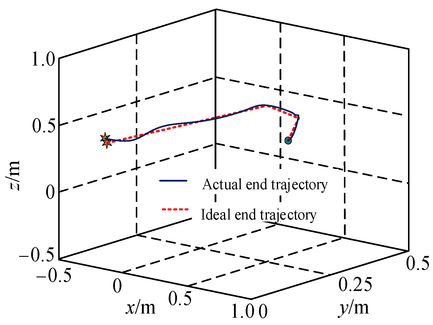
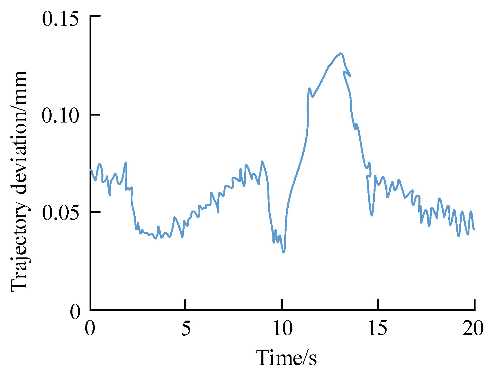
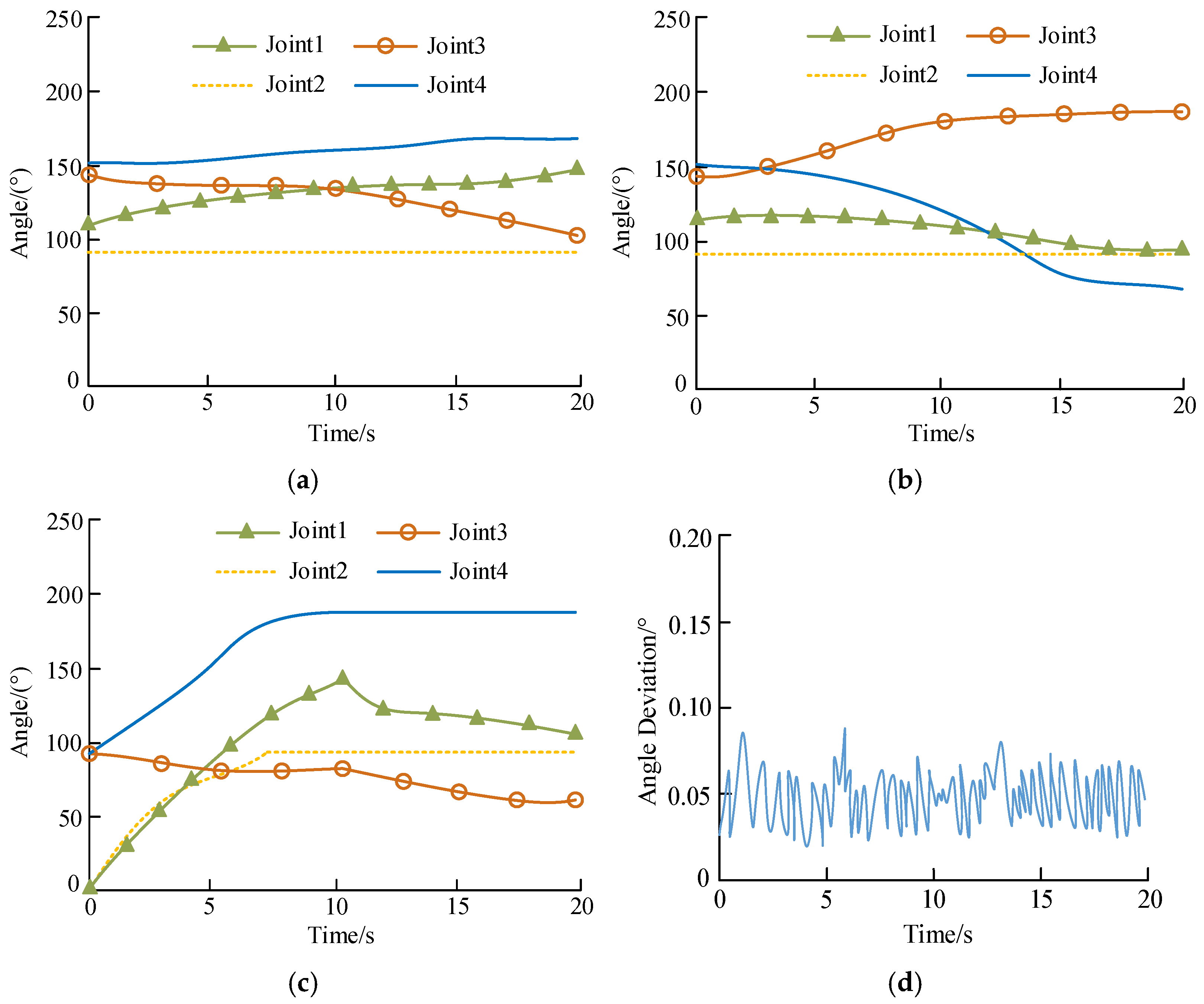
3.3. Simulation Analysis

The unfolding process of branch chain 4 is simulated. When branch chains 1, 2, and 3 and the operating object move to singularity, branch chain 2 is separated from the operating object, and branch chain 4 is unfolded and connected to the operating object to continue the operation task. The starting position and target point of branch chain 4 are set in the folding process: the starting position P_E0 = {0.1, 0.3, 0.05} of the branch-chain end point E4, and the target position P_E = {0.06, 0, 0.48}, in m. The rotary angle of the operating object is 48.5°. The simulation running time is T = 20 s, the interpolation period is ΔT = 5 ms, the maximum linear velocity is Vmax = 0.05 m/s, and the maximum rotary speed is Ωmax = 22.918°/s. The translation position error compensation coefficient is β_t = 300, and the rotary position error compensation coefficient is β_r = 100. Figure 14 shows the ideal end trajectory and the actual end trajectory of the branch-chain end point in the switching process, and the trajectory deviation is shown in Figure 15. Figure 16a,b show the joint variation curves of branch chains 1 and 2 before singularity, respectively. Branch chains 3 and 1 are symmetrically arranged, and their trends are consistent. Figure 16c shows the variation curve of each joint during the unfolding movement of branch chain 4 to the target position.

The simulation results show that the actual motion of the end point of branch chain 4 moves around the ideal trajectory in the unfolding process, and the trajectory deviation is less than 0.15 mm, which is caused by the inconsistency between the mechanical structure and the idealized motion model. In the actual structure, the position of the end point of the branch chain in the direction of the z-axis is not located at the origin of the coordinates, and the distance (d) between them is 50 mm; thus, the trajectory deviates. As shown in Figure 16d, the deviation tracking curve of the end point of branch chain 4 is calculated under the ideal model of d = 10 mm. Through a theoretical analysis, it can be seen that the closer the actual mechanical structure of the branch chain is to the ideal motion model, the smaller the corresponding end trajectory deviation; that is, the deviation decreases with a decrease in d.

In order to verify the correctness of the above theoretical calculation, in this section, a virtual prototype is established using SolidWorks 2022 to simulate the branch-chain switch, and the implementation process is shown in Figure 17. The specific planning steps are as follows:

(a) When the rotary angle of the mechanism is α = 48.5°, that is, when branch chain 2 moves to singularity, the rotary movement stops.

(b) Branch chain 4 is unfolded so it can move to the position of point E₄ by setting the joint function in the joints A₄, C₄, and D₄.

(c) By continuing to drive joints A4 and C4, branch chain 4 moves to the target contact point. Branch chain 2 is released from the operating object, and the action sequence drives joint A₂ to the position where the link A₂C₂ is coplanar with the platform and drives joint C₂ and joint D₂ so that the link C₂D₂ is perpendicular to the platform and link D₂E₂. It drives joint B₂ to return branch chain 2 to the stacked position.

(d) Branch chain 2 returns to the folded state. Branch chain 4 is connected to the operation object and maintains the rotary operation of the mechanism.

(e) The operation task is carried out under the $\cos <C_4{D}_4,D_4{E}_4>\in [-1,0]$ condition maintained by branch chain 4, and the operation object moves with a large rotary angle α of −90°.

(f) The mechanism maintains the rotary operation task until branch chain 4 moves to the set limit position.

Through the simulation results, it can be seen that, using the planned switching method, the multi-arm robot can avoid singularity when the mechanism moves to near singularity by switching the connection and releasing between the two opposite branches and the operating object. Due to each branch chain having the same structure, the mechanism still retains the same operation characteristics after switching branches, thus realizing continuous operation.

4. Conclusions

In this study, a symmetrical multi-arm robot is proposed that has four branch chains with the same structure, three of which are connected to the operating object to perform the operation task, and the fourth is used as the chain to be executed. When the branch chain approaches singularity, singularity can be avoided by releasing and connecting with the operating object, which ensures a continuous and highly accurate movement. Based on the Jacobian matrix, typical configurations of mechanisms with different singular types are obtained. According to the requirements of connection and mode switching of the branch chain, a motion planning simulation is carried out. The simulation results show that the motion plan and mode-switching design of the branch chain are feasible and correct when moving from the initial folding position to the connection position. This method can solve the problem of a small workspace of the parallel mechanism and can realize large-angle continuous rotation. In future studies, we will carry out prototype development and performance tests for this kind of mechanism to improve the design theory and analysis method.

References

1. Dai, Y.C.; Li, Z.; Chen, X.J. A Novel Space Robot with Triple Cable-Driven Continuum Arms for Space Grasping. Micromachines 2023, 14, 416. [Google Scholar] [CrossRef] [PubMed]
2. Zhang, H.; Jin, H.; Ge, M. Real-Time Kinematically Synchronous Planning for Cooperative Manipulation of Multi-Arms Robot Using the Self-Organizing Competitive Neural Network. Sensors 2023, 23, 5120. [Google Scholar] [CrossRef]
3. Liu, J.J.; Chen, Y.T.; Dong, Z.P. Robot cooking with stir-fry: Bimanual non-prehensile manipulation of semi-fluid objects. IEEE Robot. Autom. Lett. 2022, 7, 5159–5166. [Google Scholar] [CrossRef]
4. Avigal, Y.; Berscheid, L.; Asfour, T. Speedfolding: Learning efficient bimanual folding of garments. In Proceedings of the 2022 IEEE/RSJ International Conference on Intelligent Robots and Systems (IROS), IEEE, Kyoto, Japan, 23–27 October 2022; pp. 1–8. [Google Scholar]
5. McGhan, C.L.R.; Atkins, E.M. Human productivity in a workspace shared with a safe robotic manipulator. J. Aerosp. Inf. Syst. 2014, 11, 42753. [Google Scholar] [CrossRef]
6. Myron, A.; Joshua, M.; Muhammad, E. Robonaut 2-the first humanoid robot in space. In Proceedings of the IEEE International Conference on Robotics and Automation, Shanghai, China, 9–13 May 2011; pp. 2178–2183. [Google Scholar]
7. Roderick, S.; Roberts, B.; Atkins, E. The ranger robotic satellite servicer and its autonomous software-based safety system. IEEE Intell. Syst. 2004, 19, 12–19. [Google Scholar] [CrossRef]
8. David, J.C.; Ulrik, P.S.; Kasper, S. A distributed and morphology-independent strategy for adaptive locomotion in self-reconfigurable modular robots. Robot. Auton. Syst. 2013, 61, 1021–1035. [Google Scholar]
9. Saburo, M. Advanced space robot for in-orbit servicing mission. Jpn. Soc. Mech. Eng. 2003, 46, A6–A8. [Google Scholar]
10. Aghili, F.; Parsa, K. A reconfigurable robot with lockable cylindrical joints. IEEE Trans. Robot. 2009, 25, 785–797. [Google Scholar] [CrossRef]
11. Ibarkreche, J.I.; Hernández, A.; Petuya, V. A methodology to achieve the set of operation modes of reconfigurable parallel manipulators. Meccanica 2019, 54, 2507–2520. [Google Scholar] [CrossRef]
12. Corves, B.; Mannheim, T.; Riedel, M. Re-grasping: Improving capability for multi-arm robot system by dynamic reconfiguration. In Proceedings of the International Conference on Intelligent Robotics and Applications, Aachen, Germany, 6–8 December 2011; pp. 132–141. [Google Scholar]
13. Tian, C.; Zhang, D. Design and analysis of novel kinematically redundant reconfigurable generalized parallel manipulators. Mech. Mach. Theory 2021, 166, 104481. [Google Scholar] [CrossRef]
14. Tian, C.X.; Fang, Y.F.; Guo, S. Structure synthesis of reconfigurable parallel mechanisms with closed-loop metamorphic linkages. Proc. Inst. Mech. Eng. Part C J. Mech. Eng. Sci. 2018, 232, 1303–1316. [Google Scholar] [CrossRef]
15. Tian, C.X.; Xia, Z.H.; Li, L.Q. The novel synthesis of reconfigurable generalized parallel manipulators with kinematic redundancy. Mech. Mach. Theory 2024, 201, 105748. [Google Scholar] [CrossRef]
16. Tian, C.X.; Zhang, D.; Tang, H.Y. Structure synthesis of reconfigurable generalized parallel mechanisms with configurable platforms. Mech. Mach. Theory 2021, 160, 104281. [Google Scholar] [CrossRef]
17. Riedel, M.; Corves, B.; Nefzi, M. An adjustable gripper as a reconfigurable robot with a parallel structure. In Proceedings of the Second International Workshop on Fundamental Issues and Future Research Directions for Parallel Mechanisms and Manipulators, Montpellier, France, 21–22 September 2008; pp. 1–8. [Google Scholar]
18. Jin, X.D.; Fang, Y.F.; Zhang, D. Synthesis of 3-[P][S] Parallel Mechanism-Inspired Multimode Dexterous Hands With Parallel Finger Structure. J. Mech. Des. 2020, 142, 083301. [Google Scholar] [CrossRef]
19. Jin, X.D.; Fang, Y.F.; Zhang, D. Design of a class of generalized parallel mechanisms with large rotational angles and integrated end-effectors. Mech. Mach. Theory 2019, 134, 117–134. [Google Scholar] [CrossRef]
20. Zhao, F.Q.; Guo, S.; Su, H.J. Design of self-reconfigurable multiarm robot mechanism based on deployable kinematic chains. Chin. J. Mech. Eng. 2020, 33, 70. [Google Scholar] [CrossRef]
21. Xu, D.L.; Guo, S.; Zhao, F.Q. Design and Analysis of a Bimanual Parallel Dexterous Hand with Cooperative Manipulation Capability. J. Mech. Robot. 2025, 17, 061014. [Google Scholar] [CrossRef]
22. Xue, Z.H.; Liu, J.G.; Li, Y.M. Configuration Optimization of a Dual-Arm Reconfigurable Space Robot Based on Closed-Chain Inertia Matching. IEEE Trans. Autom. Sci. Eng. 2024, 1–18. [Google Scholar] [CrossRef]
23. Moosavian, A.; Xi, F.J. Design and analysis of reconfigurable parallel robots with enhanced stiffness. Mech. Mach. Theory 2014, 77, 92–110. [Google Scholar] [CrossRef]
24. Gao, F.; Li, W.M.; Zhao, X.C. New kinematic structures for 2-, 3-, 4-, and 5-dof parallel manipulator designs. Mech. Mach. Theory 2002, 11, 37. [Google Scholar] [CrossRef]
25. Gao, F.; Yang, J.; Ge, Q.J. Type synthesis of parallel mechanisms having the second class GF sets and two dimensional rotations. J. Mech. Robot. 2011, 3, 011003. [Google Scholar] [CrossRef]
26. Gosselin, C.M.; Angeles, J. Singularity analysis of closed-loop kinematic chains. IEEE Trans. Robot. Autom. 1990, 6, 281–290. [Google Scholar] [CrossRef]
27. Xu, W.; Li, C.; Liang, B. The Cartesian path planning of free-floating space robot using particle swarm optimization. Int. J. Adv. Robot. Syst. 2008, 5, 301–331. [Google Scholar] [CrossRef]
Figure 1. The schematic diagram of the proposed multi-arm robot. (a) Three branch chains connected to objects. (b) Four branch chains connected to objects.
Electronics 14 01131 g001
Figure 2. The structural diagram of the symmetrical multi-arm robot.
Electronics 14 01131 g002
Figure 3. Typical configurations in forward kinematic singularity position: (a) θ1 and θ3 are both equal to 90°; (b) α, β, and z are both equal to zero; (c) when DiEi and CiDi are coplanar; (d) values of α and β when |Jx1| = 0.
Electronics 14 01131 g003
Figure 4. Typical configurations in inverse kinematic singularity position. (a) A2C2 and C2D2 are straight and collinear; (b) AiCi and CiDi are straight and collinear.
Electronics 14 01131 g004
Figure 5. Branch-chain singularities.
Electronics 14 01131 g005
Figure 6. A mechanism rotates the operating object through chain 1 and chain 3: (a) counterclockwise rotation; (b) clockwise rotation.
Electronics 14 01131 g006
Figure 7. The configuration diagram of branch chain 2 in a singularity: (a) axonometric view; (b) front view.
Electronics 14 01131 g007
Figure 8. Configuration diagram of Type-I singularity: (a) the first configuration; (b) the second configuration; (c) front view.
Electronics 14 01131 g008
Figure 9. Branch chain 4 arrives at specified position: (a) unfolded configuration of chain 4; (b) chain 4 connects object.
Electronics 14 01131 g009
Figure 10. Branch chain 4 moves to adjacent position of contact point.
Electronics 14 01131 g010
Figure 11. Branch chain 4 is connected to the operating object. (a) Configuration I; (b) Configuration II.
Electronics 14 01131 g011
Figure 12. Structural diagram of branch chain 4 and the operating object: (a) configuration being switched; (b) the switched configuration.
Electronics 14 01131 g012
Figure 13. Typical configurations of branch chain during unfolding.
Electronics 14 01131 g013
Figure 14. End trajectory of chain 4.
Electronics 14 01131 g014
Figure 15. Trajectory deviation.
Electronics 14 01131 g015
Figure 16. Variation curve of joint angle of each branch chain: (a) articular angle in branch chain 1; (b) articular angle in branch chain 3; (c) joint angle in branch chain 4; (d) angle deviation.
Electronics 14 01131 g016
Figure 17. Simulation process of the branch-chain switching mechanism: (a) step a; (b) step b; (c) step c; (d) step d; (e) step e; (f) step f.
Electronics 14 01131 g017
Disclaimer/Publisher’s Note: The statements, opinions and data contained in all publications are solely those of the individual author(s) and contributor(s) and not of MDPI and/or the editor(s). MDPI and/or the editor(s) disclaim responsibility for any injury to people or property resulting from any ideas, methods, instructions or products referred to in the content.