Article

Collision Avoidance in Autonomous Vehicles Using the Control Lyapunov Function–Control Barrier Function–Quadratic Programming Approach with Deep Reinforcement Learning Decision-Making

Automated Driving Lab, The Ohio State University, Columbus, OH 43210, USA
*
Author to whom correspondence should be addressed.
Electronics 2025, 14(3), 557; https://doi.org/10.3390/electronics14030557
Submission received: 19 December 2024 / Revised: 28 January 2025 / Accepted: 29 January 2025 / Published: 30 January 2025
(This article belongs to the Special Issue Intelligent Technologies for Vehicular Networks, 2nd Edition)

Abstract

:
Collision avoidance and path planning are critical topics in autonomous vehicle development. This paper presents the progressive development of an optimization-based controller for autonomous vehicles using the Control Lyapunov Function–Control Barrier Function–Quadratic Programming (CLF-CBF-QP) approach. This framework enables a vehicle to navigate to its destination while avoiding obstacles. A unicycle model is utilized to incorporate vehicle dynamics. A series of simulations were conducted, starting with basic model-in-the-loop (MIL) non-real-time simulations, followed by real-time simulations. Multiple scenarios with different controller configurations and obstacle setups were tested, demonstrating the effectiveness of the proposed controllers in avoiding collisions. Real-time simulations in Simulink were used to demonstrate that the proposed controller could compute control actions for each state within a very short timestep, highlighting its computational efficiency. This efficiency underscores the potential for deploying the controller in real-world vehicle autonomous driving systems. Furthermore, we explored the feasibility of a hierarchical control framework comprising deep reinforcement learning (DRL), specifically a Deep Q-Network (DQN)-based high-level controller and a CLF-CBF-QP-based low-level controller. Simulation results show that the vehicle could effectively respond to obstacles and generate a successful trajectory towards its goal.

1. Introduction

Autonomous driving is currently a highly popular research topic in the mobility area with immense potential to enhance safety, reduce traffic congestion, and revolutionize urban transportation [1,2]. However, one of the major challenges in the development of autonomous vehicles is ensuring collision-free navigation in dynamic and unpredictable environments [3,4]. This challenge becomes particularly significant in environments ranging from multi-lane highways with fast-moving traffic [5] to crowded urban settings where vehicles must navigate amidst pedestrians [6].
Extensive research has been conducted in the field of autonomous driving to develop high-performance and robust collision-avoidance systems. Currently, most path-planning and collision-avoidance research focuses on two major approaches. The first is the optimization-based approach which frames path planning and collision avoidance as an optimization problem with well-defined constraints. The objective is to compute an optimal, collision-free trajectory by minimizing or maximizing specific objective functions. Among the various methods, the CLF-CBF-QP approach stands out as one of the most favored and widely used. This method formulates path following and collision avoidance as constraints using Control Lyapunov Functions (CLFs) for stability and Control Barrier Functions (CBFs) for safety. The optimal control is then calculated by solving a Quadratic Programming (QP) problem, ensuring both efficient and safe navigation [7,8,9,10]. Ames et al. introduced a novel framework that unified safety conditions, expressed as CBFs, with control stability objectives, represented by CLFs, within a QP setting. This framework was applied to design adaptive cruise control that balanced speed following performance with safety constraints to ensure that a vehicle maintained a safe following distance [11]. Later, Ames et al. further explored the application of CBFs in safety-critical systems and introduced two new types: reciprocal and zeroing. By integrating these functions, their methodology ensured the forward invariance of safe sets while effectively balancing safety and performance. The proposed method has been used in applications such as adaptive cruise control and lane keeping [12,13]. He et al. proposed the integration of a Finite State Machine (FSM) with the CLF-CBF-QP framework for autonomous vehicles, focusing on safe lane-change maneuvers in dynamic traffic environments. Their method ensured real-time safety constraints during lane changes [14]. Wang et al. introduced a decentralized method for ensuring collision-free operation in multirobot systems using Safety Barrier Certificates. Their approach utilizes CBFs to modify nominal controllers minimally while ensuring that safety constraints are satisfied in real-time applications [15]. Liu et al. compared potential games-based reinforcement learning and a traditional CBF-based approach for decision-making in autonomous driving. Their study highlighted that while potential games offer robustness in non-safety-conscious environments, CBFs are more computationally efficient and feasible for real-time applications [16]. Reis et al. integrated spline-based Barrier Functions for path following in multi-vehicle scenarios. Their approach integrated CLFs, elliptical CBFs, and spline-based CBFs to ensure smooth and collision-free navigation, particularly useful for highway driving with dynamic lane changes and vehicle interactions [17]. Moreover, Desai et al. introduced a CLF-CBF framework to handle nonholonomic mobile robots navigating around moving obstacles. Their approach included constraints on the steering angle to avoid impractical maneuvers, optimizing the trade-off between safety and control smoothness and achieved smooth avoidance performance [18]. Long et al. proposed a distributionally robust Lyapunov Function (LF) search method for closed-loop dynamical systems under uncertainty which can learn LFs with neural networks (NNs) [19], while Chang et al. proposed another method for learning control policies and NN-LFs which can significantly simplify the process of Lyapunov Function design and provide an end-to-end correctness guarantee [20]. Meanwhile, numerous optimization-based autonomous driving control approaches have been explored that do not rely on CLF-CBF frameworks [21,22,23,24] such as the Elastic Band algorithm [25], potential field-based approach [26], Support Vector Machine (SVM)-based approach [27], quintic spline optimization approach [28], and hybrid A* search in spatiotemporal maps [29]. However, the major limitations of the traditional optimization approach are its deficiency in real-time performance caused by its computational complexity and its shortage of control feasibility.
The second approach is the machine learning method which considers autonomous driving and collision-avoidance tasks as Markov Decision Processes (MDPs) and utilizes the reinforcement learning (RL) method to find optimal solutions. This approach makes the concurrent optimization of all processing phases possible and eventually yields superior performance. Kendall et al. pioneered the application of the DRL framework in autonomous driving, innovatively proposing an end-to-end model structure for autonomous driving [30]. Yurtsever et al. proposed an innovative hybrid deep reinforcement learning framework to develop Automated Driving Systems (ADSs) [31]. Smith et al. proposed a novel load-balancing framework that integrates CBFs with DRL to ensure both safety and efficiency in dynamic network environments. Their approach guarantees system stability by enforcing safety constraints through CBFs while DRL optimizes load distribution in real time [32]. Ashwin et al. proposed a DDPG-based sequential decision algorithm for autonomous vehicles, focusing on lane-keeping and overtaking scenarios. Their approach trains vehicles to navigate lanes, overtake static and moving obstacles, and avoid collisions, demonstrating effective performance in the TORC traffic simulator [33]. Muzahid et al. introduced a DRL-based driving strategy aimed at preventing chain collisions in autonomous traffic flow. By considering the behavior of both leading and following vehicles, their method effectively mitigates the risk of multi-vehicle collisions in high-density traffic scenarios [34]. Emuna et al. introduced a model-free DRL approach to imitate human driving behavior in collision-avoidance tasks. Their control algorithm combines model-driven rules with data-driven expert human knowledge, resulting in human-like driving policies in simulated highway scenarios [35]. Chen et al. applied a double deep reinforcement learning controller to the safety of vulnerable road users during their interactions with autonomous vehicles [5]. Albarella et al. proposed a hybrid controller that integrates DRL with Nonlinear Model Predictive Control (NMPC) for autonomous highway driving. The approach was evaluated using MATLAB and the Simulation of Urban Mobility (SUMO) traffic simulator, demonstrating robust and effective performance [36]. However, a notable disadvantage of the machine learning-based approach is the instability in model performance under normal traffic conditions due to the absence of hard-coded safety protocols. Without these predefined safety rules, the model’s actions may become unpredictable, especially in scenarios where the training data do not fully cover all possible traffic conditions. Moreover, in the DRL approach, safety is primarily ensured through the design of the reward function. Typically, a negative reward is assigned when unsafe behavior is detected, discouraging the agent from repeating such actions [37]. However, the reward setting is inherently a “soft” mechanism, as it provides guidance rather than hard constraints. It is also impractical to assign excessively large negative rewards because performing so can lead to several issues including overly conservative behaviors, sparse exploration, and instability in training.
In this paper, we propose a novel approach that combines traditional optimization-based control design with DRL to develop a high-performance and robust control strategy for autonomous vehicles. The contributions of this paper are as follows.
  • The proposed control system enables precise path tracking when no potential collisions are detected and performs effective collision avoidance when obstacles are nearby.
  • To achieve this, we first applied the CLF-CBF-QP approach to design an optimization-based path-tracking controller. The CLF constraint in the optimization ensures the stability and accurate path tracking of the autonomous vehicle, while the CBF constraint guarantees safety by preventing potential collisions between the vehicle and obstacles.
  • Building on this foundation, we integrated the traditional CLF-CBF-based control with a deep reinforcement learning algorithm for path planning.
  • The DRL algorithm generates a rough sketch of the optimal path, which the proposed optimization-based control then refines and executes.
  • To further enhance computational efficiency, a lookup table is incorporated into the CLF-CBF optimization framework, significantly accelerating the calculation process.
  • This hybrid approach leverages the strengths of both traditional control theory and modern machine learning to achieve robust, safe, and efficient autonomous vehicle operation.
The remainder of this paper is organized as follows: Section 2 introduces the methodologies employed in this study, including the unicycle vehicle dynamic model, the principles and design of the CLF and CBF, and the DRL frameworks. Section 3 presents the simulation results of the proposed algorithm, covering CLF-based path-tracking control, CLF-CBF path-tracking and collision-avoidance control for both static and dynamic obstacles, and the design of a hybrid CLF-CBF-based DRL autonomous driving agent. Detailed results and analysis are provided in this section. Finally, Section 4 concludes the paper and discusses potential directions for future work.

2. Methodology

To develop a high-performance and robust autonomous driving algorithm for navigating an autonomous vehicle from a starting point to an endpoint while performing collision avoidance as needed, we first present a simple unicycle vehicle dynamic model. After that, we introduce the basic principle of CLFs and CBFs and demonstrate how to design optimization-based control using the CLF-CBF-QP approach for autonomous vehicles. Finally, we introduce how to integrate CLF-CBF-QP control with deep reinforcement learning techniques to create a comprehensive algorithm for autonomous vehicles.

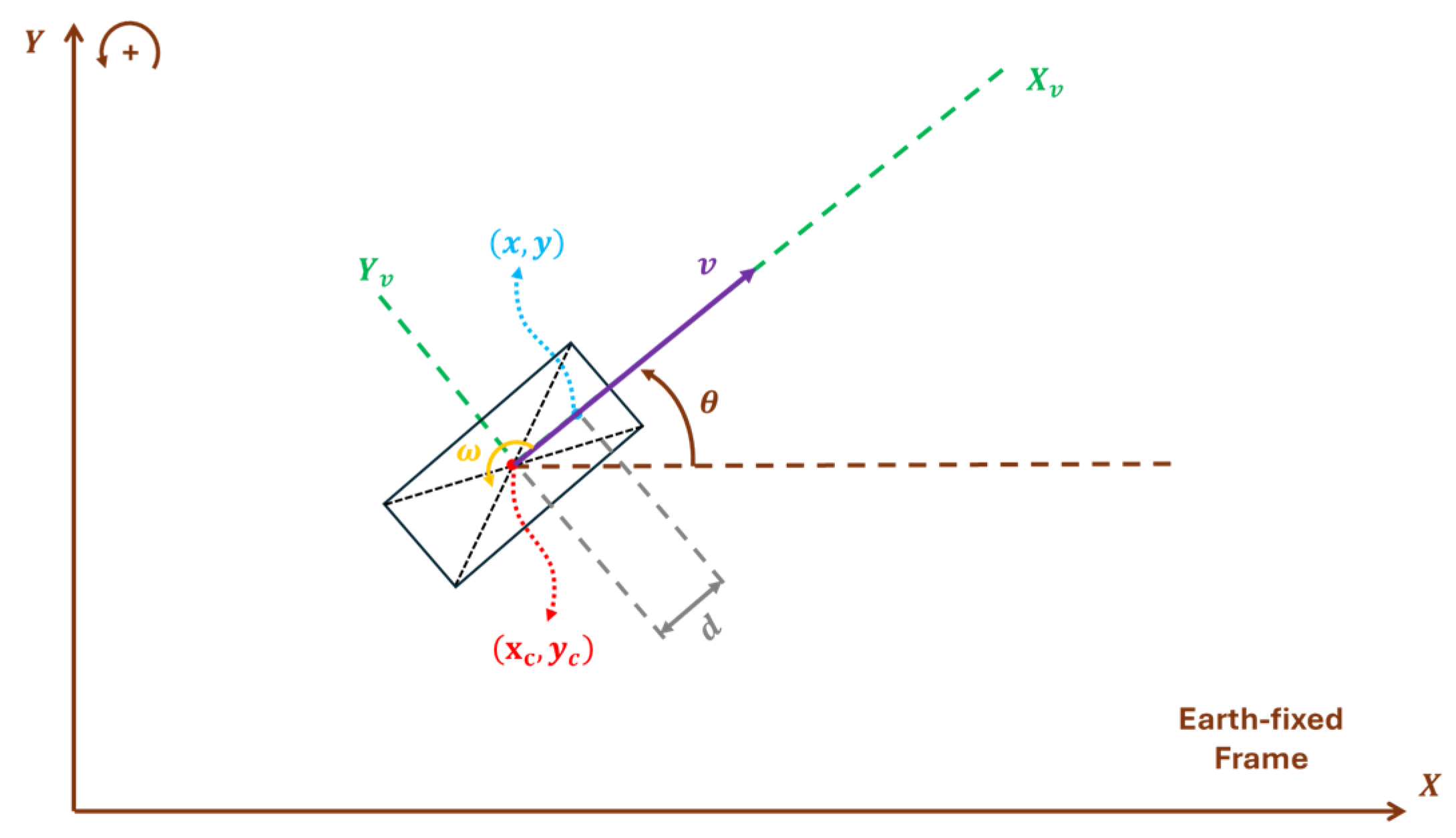
2.1. Unicycle Vehicle Dynamics

In this paper, we propose using a unicycle vehicle model for the dynamic simulation of a vehicle. Indeed, the unicycle model is widely adopted in the field of mobile robotics due to its simplicity. To achieve more realistic vehicle dynamic simulations, incorporating more complex vehicle models would be necessary. However, the use of advanced vehicle models introduces significant implementation challenges for the CLF-CBF approach and increases computational complexity. To balance real-time performance with realistic simulation, the unicycle model is used in this paper. As the simplest model, it provides a reasonable approximation of vehicle dynamics while maintaining computational efficiency. This choice aligns with many related studies, which also adopt the unicycle model to simplify the design and analysis of controllers while retaining sufficient representational fidelity for practical applications. Future work will aim to integrate more advanced vehicle models and explore efficient methods to address the associated computational challenges.
Figure 1 illustrates the plane motion of this unicycle vehicle. The vehicle can move forward with the various linear speed v and rotate with the various angular speed ω around its geometric center. Note that this is also the Dubins model of a vehicle if we fix the speed and limit the rotation angle. The state-space equation for this vehicle model is
[ x ˙ c y ˙ c θ ˙ ] = [ cos ( θ ) 0 sin ( θ ) 0 0 1 ] [ v ω ] ,
where [ x c y c ] T are the geometric center coordinates of the vehicle and θ donates the orientation of the vehicle. Now, consider another point, [ x y ] T , located in a different position along the longitudinal axis xv of the vehicle. This point is located at an offset distance, d , along the vehicle’s x-axis relative to the geometric center. The relationship between the point [ x y ] T and the vehicle’s geometric center [ x c y c ] T can be represented using the equations below.
[ x y ] = [ x c y c ] + [ cos ( θ ) sin ( θ ) sin ( θ ) cos ( θ ) ] [ d 0 ]
The state-space equation for the geometric center of the vehicle is given by
[ x ˙ y ˙ θ ˙ ] = [ cos ( θ ) d sin ( θ ) sin ( θ ) d cos ( θ ) 0 1 ] [ v ω ] .
Both state-space Equations (1) and (3) are driftless nonlinear systems which rely entirely on control inputs to define their motion. They are particularly useful for autonomous driving research, as they simplify the analysis and synthesis of control laws without the need to counteract drift dynamics. Moreover, the simplicity of the unicycle model largely simplifies the design of Control Lyapunov Functions and Control Barrier Functions by streamlining the calculations. For realistic simulation, we constructed the model in both Python 3.13 and Simulink 2024a for MIL and real-time MIL simulation. The simulation setting and results are presented in the Results Section.

2.2. Control Lyapunov Functions and Control Barrier Functions

2.2.1. Control Lyapunov Functions’ Principle and Design

The CLF is usually used as a constraint of an optimization problem to ensure the stability of dynamic systems by defining a scalar function that decreases over time as the system evolves. By encoding stability criteria into a function, the CLF allows the system to converge to the desired state with reasonable speed despite dynamic and environmental uncertainties. In autonomous driving, a CLF is employed to design a path-tracking controller that guides the vehicle towards the desired target position. This approach is robust in real-time applications where stability must be maintained even in the presence of disturbances, ensuring that the autonomous vehicle operates reliably and efficiently. Through CLF-based control strategies, vehicles can achieve precise trajectory tracking even in complex driving scenarios, which makes it a foundational element in advanced autonomous driving algorithms.
Let us first introduce the basic principle of the CLF. Consider the control affine system given by
x ˙ = f ( x ) + g ( x ) u
where x is the state vector, u is the control input vector, and f and g are Lipschitz continuous in x . f is the uncontrolled part, which represents the system’s natural dynamics, while g is the control distribution matrix which determines how the control inputs influence the system’s dynamics. Let V ( x ) :   R n R be a continuously differentiable function; the CLF V ( x ) satisfies the following:
(1)
Positive definiteness:
V ( x ) > 0   for   all   x x e ,   and   V ( x e ) = 0
where x e is the equilibrium point.
(2)
Sublevel set boundedness: For a given constant, c > 0 , the sublevel set Ω c = { x   ϵ   R n :   V ( x ) c } is bounded. This ensures that V ( x ) defines a meaningful region of attraction (ROA) around x e .
(3)
Stability: there exists a control input, u   ϵ   R n , such that the derivative of V ( x ) along the trajectory of the system satisfies
min u ϵ U V ˙ ( x , u ) = min u ϵ U   [ V ( x ) · ( f ( x ) + g ( x ) u ) ] < 0 ,         x   ϵ   Ω c \ { x e }
In this paper, a CLF is applied to design the path-tracking controller, ensuring that the vehicle accurately follows a predefined trajectory. Equations (7) and (8) demonstrate the design of a Lyapunov Function and its derivative where e is the path-tracking error. The path-tracking error can be calculated using the position of the vehicle and the position of the tracking point on the path, e = p p d ( γ ) , where p d ( γ ) : 2 represents the planar parameterized path, generated by B-spline fitting, for example, and γ is a time-dependent parameter for the position along the path. Equation (6) demonstrates the dynamics of the path where the desired path speed is γ d and g ( e ) is used to slow down the tracking point when the path-tracking error is too large. The CLF incorporates the path-tracking error, quantifying the deviation of the vehicle from the desired path. By integrating the CLF as a constraint within the Quadratic Programming (QP) optimization problem, the controller ensures that the system minimizes the path-tracking error in every time step. This formulation guarantees stability by driving the CLF to decrease over time, ultimately forcing the vehicle to converge to the predefined path. The detailed design of the CLF is illustrated in Equation (10) where ϵ is the relaxing term which indicates that the vehicle can temporarily deviate from the path when necessary.
V ( e ) = 1 2 e 2
V ˙ ( e ) = e T ( [ cos ( θ ) d sin ( θ ) sin ( θ ) d cos ( θ ) ] u p d γ γ ˙ )
γ ˙ = γ d + g ( e )  
e T ( [ cos ( θ ) d sin ( θ ) sin ( θ ) d cos ( θ ) ] u p d γ γ ˙ ) + α 2 e 2 ϵ

2.2.2. Control Barrier Functions’ Principle and Design

The Control Barrier Function (CBF) is usually used as a constraint in an optimization problem to ensure the safety of dynamic systems. A CBF defines a safe set which is a region in the state-space where the system can operate without violating safety conditions. By incorporating CBF constraints into optimization-based controllers, the controller ensures that the system remains within the defined safe set while allowing flexibility for other objectives such as stability or performance. In the context of autonomous driving, CBFs are usually employed to guarantee collision avoidance, maintain lane adherence, and respect speed limits. In this paper, we use a CBF to enforce minimum distance constraints between the autonomous vehicle and obstacles, ensuring safe operation in dynamic environments. By integrating CBFs with other constraints such as CLFs, an optimization-based control strategy can be designed for autonomous vehicles. This approach enables the simultaneous achievement of safety, efficient path tracking, and effective collision avoidance.
For the CBF, let h ( x ) :   R n R be a continuously differentiable function that defines the safe set
C = { x   ϵ   R n :   h ( x ) 0 }
where h ( x ) 0 represents the safe region and h ( x ) < 0 represents the unsafe region. The function h ( x ) is considered a CBF if there exists a control input, u   ϵ   R n , such that the following condition holds for all x   ϵ   C .
s u p u ϵ U [ h ( x ) x · ( ( f ( x ) + g ( x ) u ) ] α ( h ( x ) )
where α is a class- κ function, which specifies the rate at which the system can approach the boundary of the safe set.
In this paper, the CBF is utilized to design the collision-avoidance controller, ensuring the vehicle’s safety in the presence of nearby obstacles. To simplify the problem and enable an effective mathematical formulation, we assume that both the vehicle and obstacles have elliptical geometries. This assumption allows the use of an ellipse-based Barrier Function, which defines a safe region by ensuring that the vehicle maintains an appropriate distance from obstacles. By assuming that both the vehicle and obstacles have elliptical geometries, we imply that they can be approximated or enclosed by one or more elliptical shapes, depending on the complexity of their structures. Once these elliptical boundaries are established, elliptical CBF constraints can be applied, with each boundary corresponding to a specific CBF constraint, to formulate the QP problem. This approach enables the efficient calculation of the optimal control.
The primary purpose of utilizing CBFs is to ensure collision avoidance and maintain safety during path tracking. In our simulation, both the vehicle and obstacles are encircled with elliptical boundaries. CBFs are employed to guarantee that the vehicle’s boundary does not overlap with the obstacle boundaries, effectively preventing collisions. If there is more than one obstacle, each obstacle/boundary corresponds to a specific CBF constraint. While it is possible to impose input constraints by introducing additional constraints into the QP formulation, this approach significantly increases the problem’s complexity and computational time. To address this, our method solves the CLF-CBF-QP problem without input constraints and applies saturation directly during the execution of the calculated optimal input. This approach maintains computational efficiency while ensuring practical feasibility.
Equation (13) is the Barrier Function of an elliptical region with H ( θ ) = R ( θ ) Λ R ( θ ) T and Λ = diag { 1 / a 2 ,   1 / b 2   } where R ( θ ) is the 2D rotational matrix. The constants a and b are the longest and shortest radii of the ellipse. The center of this elliptical region is located at p c , the orientation of the region is θ , and the position of a random point is δ . This equation is used to determine whether a given point lies within the elliptical region. Equation (14) represents the boundary of the aforementioned elliptical region where ρ is the rotation angle between 0 and 2 π . Equation (15) demonstrates the design of the Barrier Function between two arbitrary elliptical regions, i and j, where h i represents the Barrier Function of the elliptical region i, j ( ρ ) represents the boundary function of the elliptical region j, and ξ c i , ξ c j represent the position and orientation of the two elliptical regions. By incorporating this Barrier Function into the control framework, the vehicle can dynamically adjust its trajectory to avoid collisions while preserving stability and operational efficiency. The detailed design of the CBF is illustrated in Equation (16).
h ( δ ) = 1 2 ( δ p c ) H ( δ p c ) 1 2
( ρ ) = [ a cos ( ρ ) cos ( θ ) b s i n ( ρ ) sin ( θ ) + x c a cos ( ρ ) sin ( θ ) + b s i n ( ρ ) cos ( θ ) + y c ]
h i j ( ξ c i , ξ c j ) = min ρ ϵ h i ( j ( ρ ) )
h i j ξ c i g c ( ξ c i ) u i + h i j ξ c j g c ( ξ c j ) u j + β h i j ( ξ c i , ξ c j )   0

2.2.3. CLF-CBF-QP Formulation

After designing the appropriate CLF and CBF constraints for the optimization-based controller, the next step was to formulate the CLF-CBF-QP framework. The complete formulation of the CLF-CBF-QP is presented in Equation (17).
u = arg min u , ϵ   u 2 + q ϵ 2
s . t       V ˙ ( ξ i , u i ) + α V ( ξ i ) ϵ   and
h ˙ i j ( ξ c i , ξ c j , u i , u j ) + β h i j ( ξ c i , ξ c j )   0 ,   f o r   j = 1 N
where ξ c i , ξ c j represent the position and orientation of the elliptical regions corresponding to the vehicle and obstacles, respectively. The index i refers to individual vehicles, while j corresponds to individual obstacles. The constants α and β are designed to ensure that the system converges to the optimal control solution at an exponential rate. ϵ is the relaxing term which indicates that the vehicle can temporarily deviate from the path when necessary. Additionally, q is a positive constant introduced to penalize the relaxation of the CLF constraint, thereby encouraging adherence to the desired trajectory. By solving this optimization problem, the autonomous vehicle can effectively avoid potential collisions with obstacles, achieve accurate path tracking to the greatest extent possible, and minimize control effort while ensuring efficient and safe navigation.

2.3. Deep Reinforcement Learning

A Markov Decision Process (MDP) is a mathematical framework for modeling sequential decision-making in situations where outcomes are uncertain. It is defined by four key components: the state, actions, transitions, and rewards. The goal in a Markov Decision Process is to find an optimal policy that can maximize the cumulative reward. Autonomy can be viewed as inherently being an MDP problem, as it requires continuous decision-making in a highly uncertain and dynamic traffic environment. This means that the system must account for evolving traffic conditions, unpredictable obstacles and vulnerable road users (VRUs), and complex interactions with other road users while making sequential decisions to achieve safe and efficient navigation. The state includes information like the vehicle’s position, speed, and surrounding environmental information. The actions represent the vehicle’s control decisions, such as acceleration, braking, or steering. The transition probabilities capture both the dynamics of vehicle and traffic environment, determining how the traffic environment and vehicle’s state evolve based on its actions. A reward function can guide the vehicle to achieve objectives like reaching a destination efficiently and safely. Moreover, the decision-making process satisfies the Markov property which means that the decision-making process and state transitions depend solely on the current state and action, without requiring knowledge of the past. Due to these characteristics, DRL has emerged as a promising tool for tackling this challenge. DRL has been extensively researched for developing advanced driver-assistance systems (ADASs), leveraging its ability to learn optimal policies directly from interactions with the environment. Currently, most research focuses on end-to-end DRL approaches where raw sensor inputs, such as images or videos, are directly processed to generate control commands for the vehicle. For instance, an autonomous vehicle may use camera images to predict steering angles or acceleration commands. This approach has several advantages; it simplifies the optimization process by avoiding the need for intermediate steps, such as feature extraction or trajectory planning, and allows the system to optimize all stages of decision-making and control simultaneously in a unified framework. Additionally, end-to-end methods are usually model-free and can adapt to complex scenarios by learning directly from large-scale data, capturing patterns that may be difficult to model explicitly.
However, the end-to-end DRL approach also presents significant limitations. One major drawback is the requirement for extensive computational resources to train the DRL agent effectively, often requiring large datasets and substantial training time. Another critical issue is the difficulty of incorporating hard-coded safety rules into the learned policy. While DRL excels at finding solutions that work well in training environments, it may fail to ensure safety under untrained or extreme conditions, which is unacceptable for real-world autonomous driving applications. These limitations highlight the need for a hybrid approach that combines the strengths of DRL with traditional optimization-based control methods.
To address these challenges, we propose a novel framework that integrates DRL with traditional CLF-CBF-based control. In this hybrid framework, DRL is utilized for high-level decision-making, such as generating rough path plans and determining strategic maneuvers based on environmental conditions. This enables the system to leverage DRL’s data-driven capabilities for better decision-making and adaptability in complex and uncertain environments. On the other hand, CLF-CBF-based control is responsible for refining and executing planned paths, ensuring the vehicle’s stability, safety, and efficiency during operation. By separating high-level decision-making from low-level control, this approach combines the flexibility and learning capabilities of DRL with the robustness and safety guarantees provided by traditional control techniques. This hybrid method not only addresses the limitations of end-to-end DRL approaches but also ensures that the autonomous vehicle can operate reliably and safely in a wide range of scenarios while benefiting from the strengths of both methodologies.
DRL can be broadly categorized into two methods: the value-based approach and policy-based approach. Value-based DRL, inspired by Q-learning [15], focuses on estimating the value of different actions to determine the best one. The Deep Q-Network (DQN) and its successor [16,17,18,19] extend this by using neural networks to approximate Q-values in environments with large state spaces. On the other hand, policy-based DRL methods directly learn the policy, which maps states to actions without explicitly estimating value functions. Policy Gradient (PG) methods, inspired by REINFORCE [20], Actor-Critic [21], such as A2C and A3C [22], PPO [23], and their successors [24,25,26], optimize a policy by adjusting its parameters in the direction that maximizes expected rewards. Both approaches in DRL are widely utilized in the field of autonomous driving [27,28,29,30].
In this paper, we propose using the DQN framework to design high-level control for autonomous driving. The DQN, as a value-based reinforcement learning algorithm, offers several advantages over policy-based algorithms. It is computationally efficient, particularly for discrete action spaces, and can achieve stable convergence with techniques like experience replay and target networks. These properties make the DQN an ideal choice for handling high-level decision-making in structured environments. To implement this, we converted the driving environment into a grid map, where the map is divided into discrete grids. Each grid represents a specific location, with grids containing the destination and obstacles distinctly marked. In each time step, the DQN framework determines a high-level decision, guiding the vehicle to move to a nearby grid based on its learned policy. The CLF-CBF controller then executes these high-level decisions, refining the vehicle’s trajectory and ensuring stability, safety, and efficiency throughout the process. This combination of the DQN for decision-making and CLF-CBF for control execution ensures a robust and effective approach to autonomous driving in dynamic environments.
Figure 2 illustrates an example of a traffic environment which can be used to train a DRL-based high-level decision-making agent. The yellow grid represents the vehicle’s current position, while the red grid indicates the presence of a dynamic obstacle. The green grid marks the destination. The vehicle’s objective is to navigate around the dynamic obstacle and reach the destination as quickly as possible. The DRL-based high-level decision-making agent is responsible for generating basic navigation commands, such as moving to the grid above or below the current position. These commands serve as guidance for the overall trajectory planning. The CLF-CBF-QP-based low-level controller, in turn, interprets and executes these commands with precision, ensuring smooth and safe motion while adhering to vehicle dynamics and avoiding collisions. This hierarchical structure enables the seamless integration of high-level strategic decision-making with low-level control execution, providing both flexibility and robustness in navigation.
Figure 3 demonstrates how to use the CLF-CBF controller to execute high-level steps generated by the DRL agent. Each high-level decision corresponds to a unique trajectory. After the DRL-based high-level controller decides, the CLF-CBF controller ensures that the vehicle moves from the center of the current grid to the center of the next grid. Notably, there are two possible ways to move to the grid behind the vehicle: either a left turn or a right turn, both of which are feasible. To handle such scenarios, an additional rule-based algorithm can be incorporated to select the optimal path based on specific conditions. Furthermore, the DRL controller may occasionally decide that the vehicle should remain stationary. If the DRL chooses not to move, the low-level controller will maintain the vehicle’s position until the next time step.
Algorithm 1 demonstrates the DQN framework that was used to train the autonomous driving high-level decision-making agent in this paper. The Q-value, also known as the action value, represents the expected cumulative reward that an agent can obtain by starting from a specific state, s , and then taking a specific action, a . In the DQN, a neural network approximates the Q-value function. The network takes the current state s as the input and outputs vectors of Q-values, one for each possible action in the action space. The update equation of the Q-value function essentially updates the parameter in the neural network. The Q-value function is updated using the Bellman equation, where the target Q-value is calculated as the immediate reward plus the discounted maximum Q-value of the next state (lines 12 and 14 in Algorithm 1). This update process adjusts the parameters of the neural network through gradient descent, minimizing the loss between the predicted Q-value and the target Q-value, thereby enabling the network to learn and improve its approximation of the optimal Q-value function.
Algorithm 1: DQN algorithm flowchart.
1: Initialize replay memory D
2: Initialize target network Q ^ and Online Network Q with random weights θ
3: for each episode do
4:     Initialize traffic environment
5:     for t = 1 to T do
6:         With probability ϵ select a random action a t
7:         Otherwise select a t = max a Q ( s t , a ; θ )
8:         Execute a t in CARLA and extract reward r t and next state s t + 1
9:         Store transition ( s t , a t , r t , s t + 1 ) in D
10:       if t mod training frequency == 0 then
11:             Sample random minibatch of transitions ( s j , a j , r j , s j + 1 )) from D
12:             Set y j = r j + γ max a Q ^ ( s j + 1 , a ) ; θ )
13:             for non-terminal s j + 1
14:             or y j = r j   for terminal s j + 1
15:             Perform a gradient descent step to update θ
16:             Every N steps reset Q ^ = Q
17:         end if
18:         Set s t + 1 = s t
19:     end for
20: end for
Figure 4 demonstrates the structure of the neural network used in the DQN framework. The neural networks used in this paper are feedforward neural networks. The proposed DQN agent contains two fully connected hidden layers that each contain 32 neurons. The corresponding activation function for the hidden layer is ReLU. The learning rate for training is set to 0.001, using the Adam optimizer, and the model evaluates training performance using the mean absolute error (MAE) metric. The agent undergoes 1000 warm-up steps before learning and updates the target network with a rate of 0.01.
The neural network in Figure 4 is a deep neural network. The distinction between shallow and deep neural networks depends on the number of hidden layers; shallow neural networks typically contain only one hidden layer, while deep neural networks have two or more hidden layers. Whether a shallow neural network or deep neural network is appropriate depends largely on the complexity of the task. Neural networks with two hidden layers are very common in research and often strike a balance between simplicity and performance. In our research, the environment is relatively simple, with a small grid map and a limited action space. The deep neural network with two hidden layers is sufficient to capture the necessary features of this environment. Additionally, because the neural network used is simple, the training complexity is low, requiring less computational power and a smaller amount of data. This simplicity also minimizes the risk of overfitting, making it an efficient choice for this task. In practical applications, if this method were to be used in a more complex environment—such as one with a larger map size or a more diverse action space—a more sophisticated neural network architecture would be required. This might involve convolutional layers or vision transformer layers for feature extraction and perception. However, for the given task, the current network design is both sufficient and computationally efficient.

3. Results

In this section, we present the simulation results of the proposed controller to evaluate its performance and robustness. First, the CLF-based path-tracking simulation results are shown, highlighting the controller’s ability to achieve precise path tracking under normal conditions. Next, the simulation results of the CLF-CBF-based autonomous driving controller are shown for scenarios involving both static and dynamic obstacles. These results illustrate the vehicle’s capability to maintain precise path tracking during normal traffic conditions and effectively execute collision-avoidance maneuvers in emergency situations. Finally, we present the simulation results of the hybrid framework, where the DQN-based high-level decision-making agent was combined with the CLF-CBF-based low-level controller. These results demonstrate how integrating traditional optimization-based controllers with deep reinforcement learning can significantly enhance the autonomous driving capabilities of vehicles, enabling better decision-making and improved driving safety in complex traffic environments. Moreover, all the test conditions were initially evaluated using simulations within a Python-based environment. These simulations were then followed by Simulink-based real-time model-in-the-loop (MIL) simulations, which validated the real-time capabilities of the proposed controller. This two-stage testing process ensured both the feasibility and practicality of the controller in dynamic and real-time scenarios.

3.1. CLF-CBF-Based Optimization Controller

In this section, simulations of the CLF-CBF-based autonomous driving controller are discussed. The vehicle started at a designated initial position and had to navigate to the given destination. The original path, which was pre-calculated, included obstacles along the way. The objective of the simulation was to evaluate whether the controller could effectively perform collision avoidance near obstacles while maintaining accurate path tracking to the greatest extent possible.

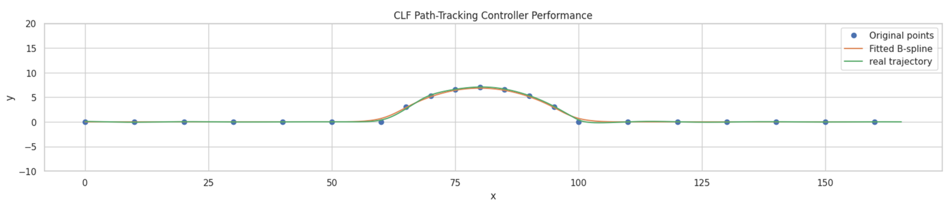
3.1.1. CLF-Based Path-Tracking Controller

Figure 5 shows the real-time MIL simulation results of the CLF-based path-tracking controller. In the figure, the XY coordinates represent a bird’s-eye view map of the testing traffic conditions, with the units for both the x- and y-axes being meters. The figure illustrates that the vehicle followed the desired path with high precision under most conditions, demonstrating the controller’s effectiveness in path-tracking tasks. However, a slight deviation from the original path is observed in regions with higher curvature, where tracking accuracy decreases marginally. This minor deviation could be attributed to the dynamic complexity introduced by the path’s curvature, which challenged the controller’s ability to maintain perfect alignment. Despite these small discrepancies, the overall performance of the CLF-based path-tracking controller was robust, showing its capability to handle real-time scenarios effectively while maintaining accurate path tracking. Further refinements or adjustments may help address the minor tracking offsets in the curved sections to improve performance further. Figure 6 shows the steering angle response, θ , of the vehicle over time during the simulation. The plot indicates that the controller maintained stable steering behavior throughout the scenario.

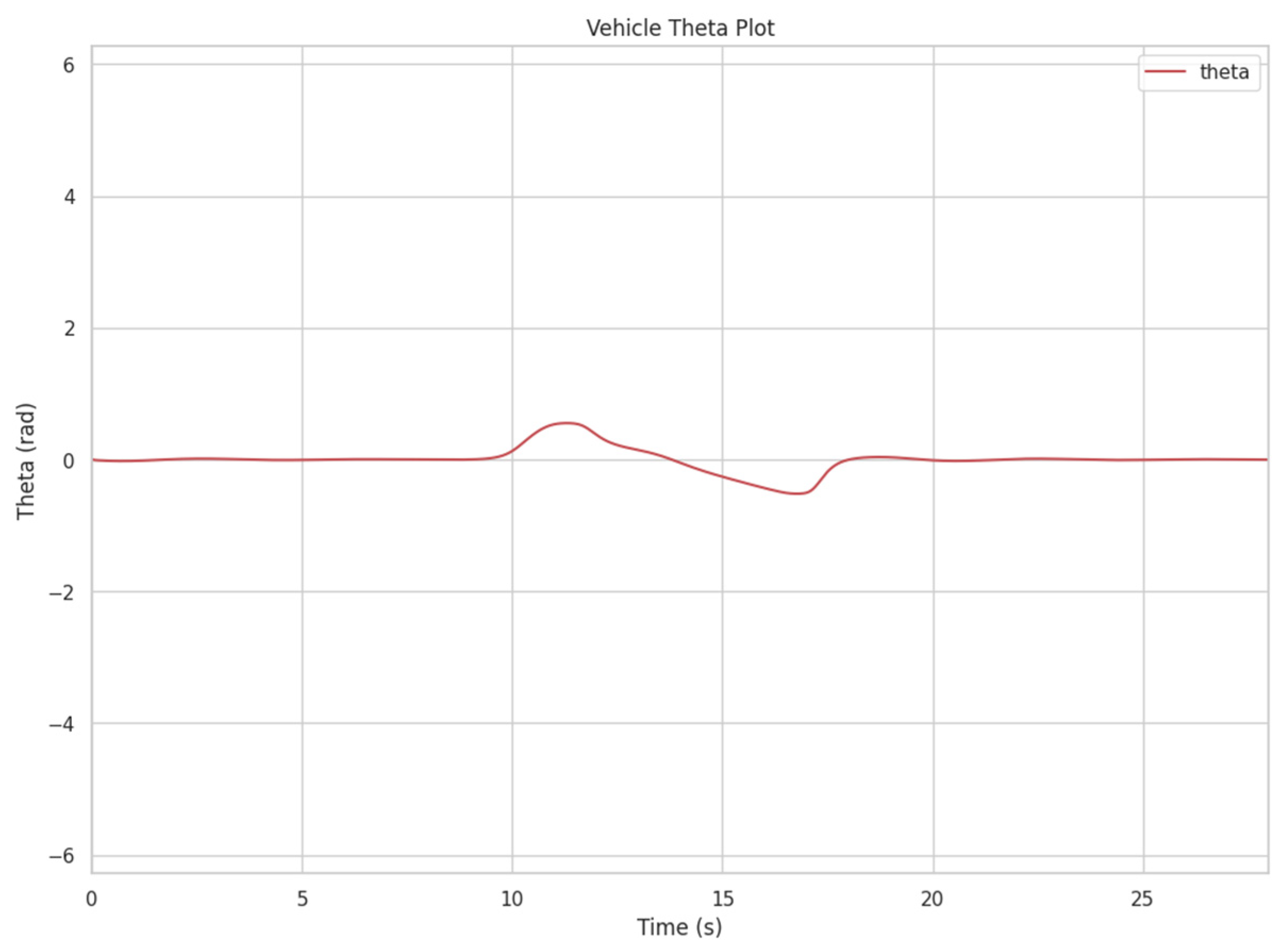
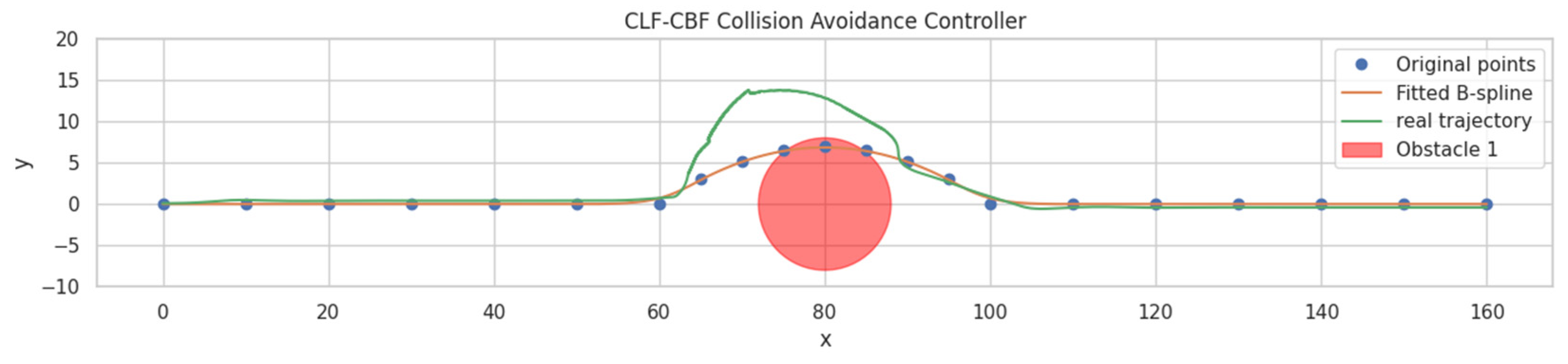
3.1.2. CLF-CBF-Based Autonomous Driving Controller for Static Obstacle

Figure 7 illustrates the simulation results of the CLF-CBF-based autonomous driving controller in an environment with a static obstacle. In the figure, the XY coordinates represent a bird’s-eye view map of the testing traffic conditions, with the units for both the x- and y-axes being meters. The figure marks the original path waypoints in blue dots, the fitted B-spline trajectory in orange, and the vehicle’s actual trajectory in green. The presence of an obstacle, marked as a red circle, required the vehicle to deviate from the original path to avoid a collision. The simulation demonstrated that the controller successfully adjusted the vehicle’s trajectory while maintaining safe navigation around the obstacle. This result highlights the controller’s ability to combine path tracking with collision avoidance effectively. The smooth transitions and minimal deviation from the intended path illustrate the robustness of the CLF-CBF framework in handling static obstacles. Figure 8 shows the steering angle response, θ , of the vehicle over time during the simulation. The plot indicates that the controller maintained stable steering behavior throughout the scenario. During the initial phase, slight oscillations in the steering angle could be observed as the vehicle adjusted to follow the desired trajectory and avoid the static obstacle. These oscillations diminished over time, and the steering angle stabilized as the vehicle returned to the planned path after bypassing the obstacle. These results demonstrate the controller’s ability to make precise adjustments while ensuring stability and smooth operation, even in scenarios requiring significant maneuvering. The demo video link of this scenario is attached at the end of this paper.

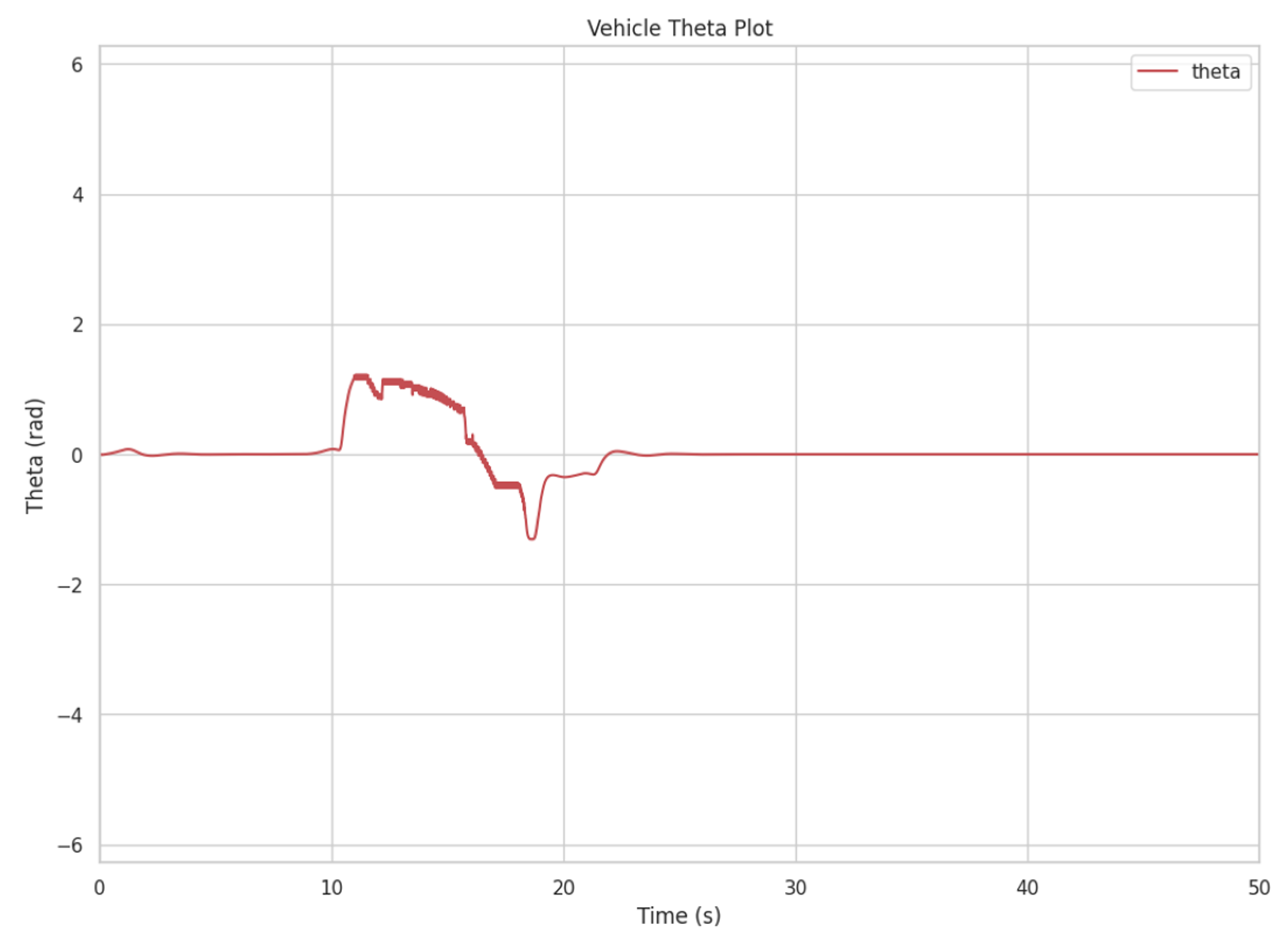
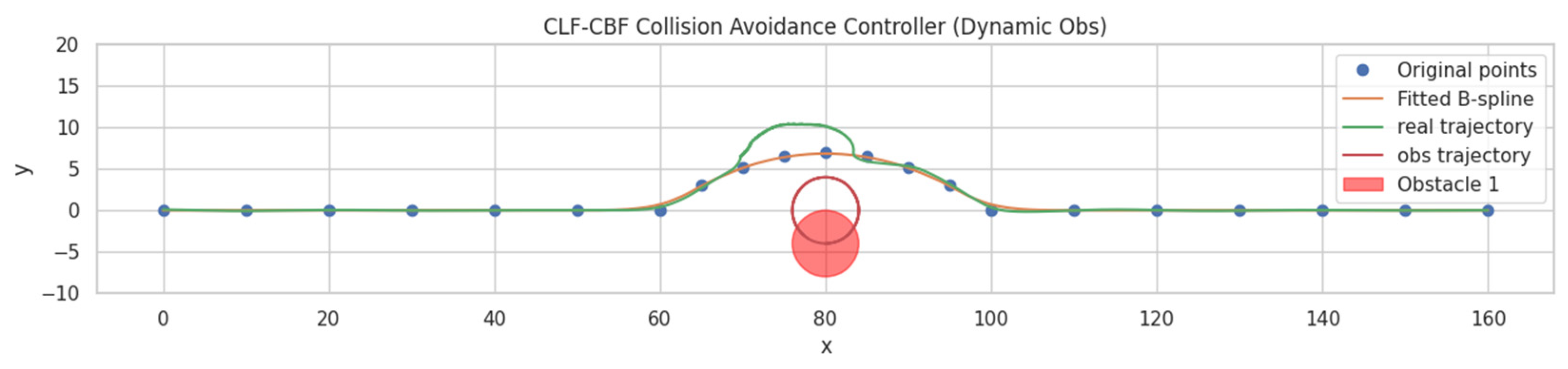
3.1.3. CLF-CBF-Based Autonomous Driving Controller for Dynamic Obstacle

Figure 9 presents the simulation results of the CLF-CBF-based autonomous driving controller in an environment with a dynamic obstacle. In the figure, the XY coordinates represent a bird’s-eye view map of the testing traffic conditions, with the units for both the x- and y-axes being meters. The original path waypoints are marked with blue dots, the fitted B-spline trajectory is in orange, and the vehicle’s actual trajectory is in green. A dynamic obstacle, represented as a red circle, moved in a circular pattern. When the obstacle moved to the top and blocked a section of the pre-planned trajectory, the vehicle was required to deviate from the original path to avoid a collision. The simulation results demonstrate the controller’s ability to adjust the vehicle’s trajectory dynamically, ensuring safe navigation around the obstacle. The smooth transitions and minimal deviation from the intended path highlight the robustness of the CLF-CBF framework in handling dynamic obstacles effectively. Additionally, Figure 10 illustrates the vehicle’s steering angle response, θ , over time during the simulation. The plot reveals stable steering behavior throughout the scenario, with minor oscillations in the middle phase as the vehicle adjusted to the desired trajectory while avoiding the obstacle. The demo video link of this scenario is attached at the end of this paper.

3.2. Hybrid DRL- and CLF-CBF-Based Controller

In this section, simulations of the hybrid DRL- and CLF-CBF-based autonomous driving controller are presented. The vehicle started in a designated initial position and needed to navigate to a specified destination, with a freely moving obstacle present in the environment. There was no pre-calculated path between the initial position and the destination. Instead, the high-level DRL agent dynamically calculated a rough path based on the vehicle’s status and the surrounding traffic conditions, while the low-level CLF-CBF-based controller executed the agent’s decisions. The objective of the simulation was to evaluate whether the controller could effectively perform collision avoidance and ensure safe navigation in a dynamic environment.
In this paper, the state representation includes the distance between the vehicle and the obstacle, as well as the distance between the vehicle and the destination. The action space consisted of four possible movements: forward, backward, left, and right. A positive reward of +25 was assigned when the vehicle successfully reached the destination grid. Conversely, a large negative reward of −300 was imposed if the vehicle collided with an obstacle by entering its grid. Additionally, a small negative reward of −1 was applied for every move to encourage the vehicle to reach the destination as quickly as possible, promoting efficient navigation.

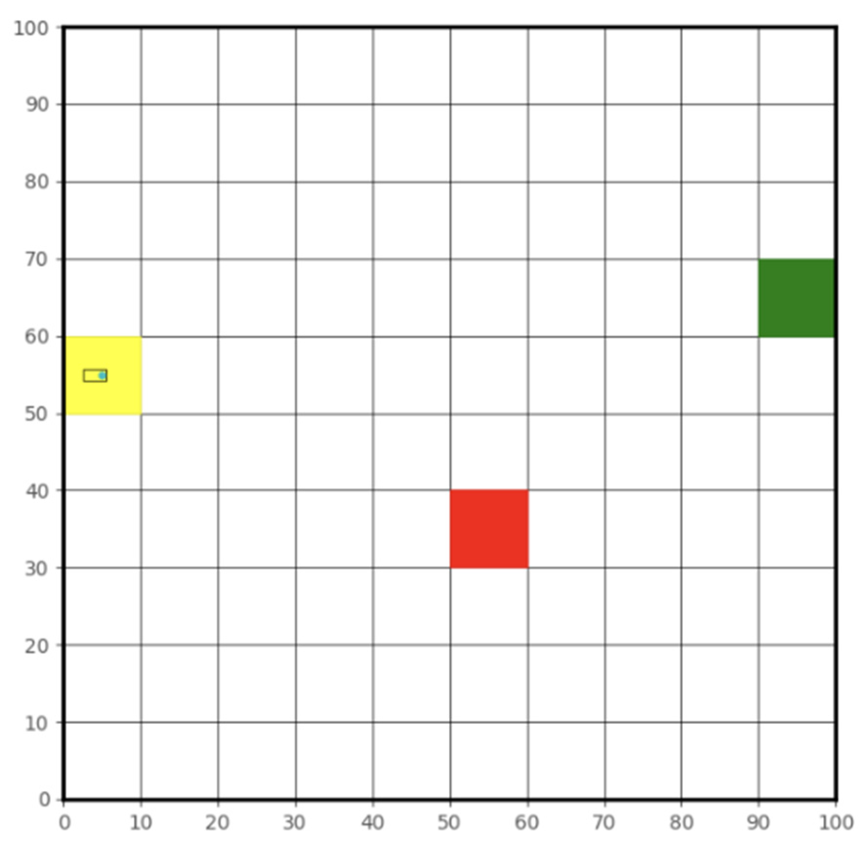
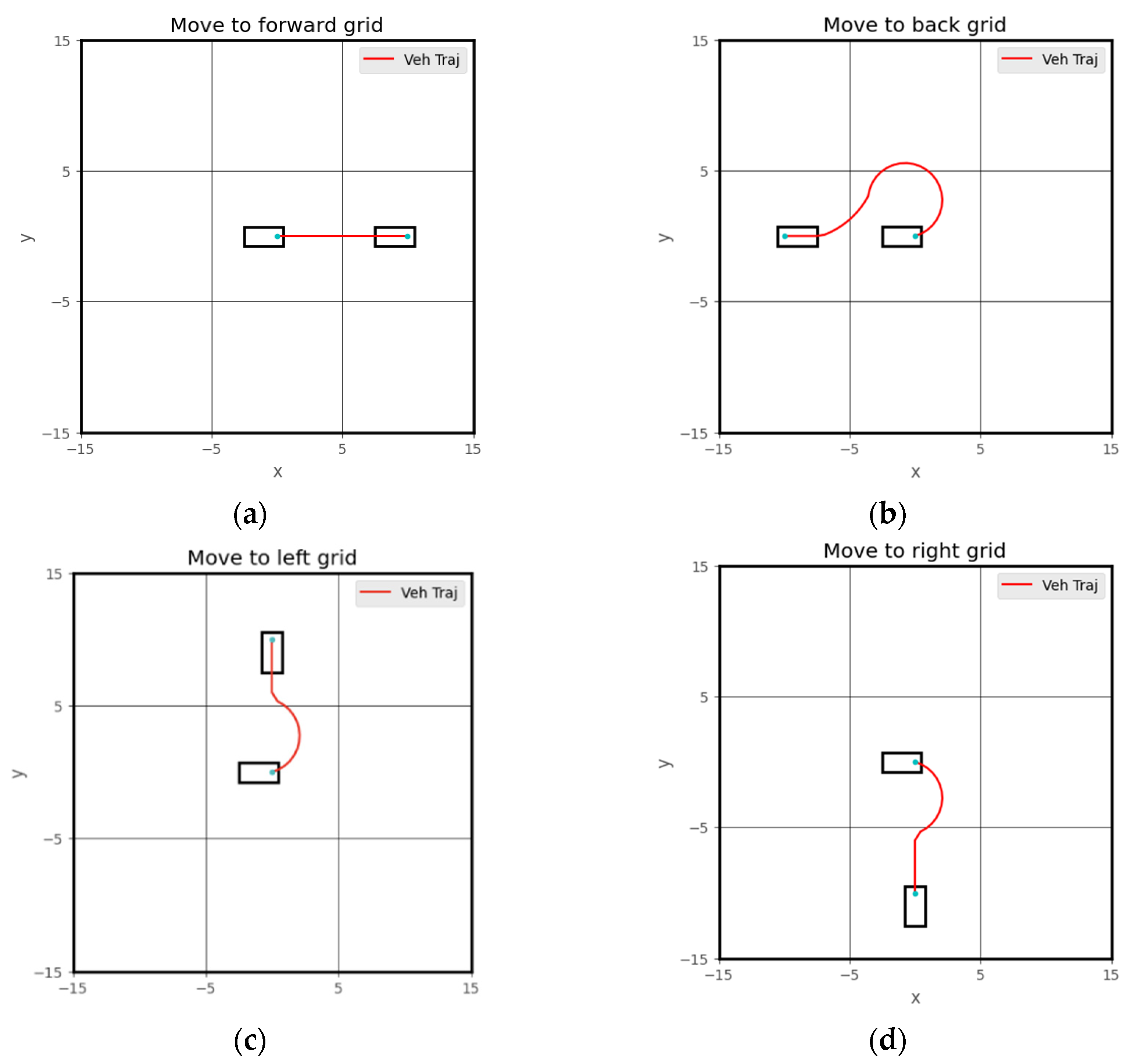
3.2.1. DRL High-Level Decision-Making Agent

Figure 11 demonstrates the training process of the proposed DRL high-level decision-making agent, which indicates significant improvements in the agent’s performance over time. The reward plot shows a sharp increase during the early stages, starting from a highly negative value −6.2 and stabilizing near 0.5 after 300,000 steps, indicating that the agent quickly learned a basic policy and continued to refine it. The loss decreases rapidly from an initial high value 106 to a more stable range after 100,000 steps, with minor fluctuations throughout the end, which reflects that the agent could effectively minimize the prediction error. Similarly, the mean Q-values show a notable increase, transitioning from early negative values to a stable value range around 20 after 100,000 steps. This demonstrates improved confidence in the action value estimations. Together, these three plots indicate the agent’s ability to effectively learn and optimize its policy, balancing exploration and exploitation to achieve improved performance as training progresses. The minor fluctuations in loss and reward suggest that further fine-tuning may still enhance stability and performance.
Figure 12 demonstrates an example of the proposed DRL high-level decision-making agent. In the figure, the XY coordinates represent a bird’s-eye view map of the testing traffic conditions, with the units for both the x- and y-axes being meters. The blue line indicates the trajectory of the proposed agent, and the red line indicates the motion of the obstacle. It is shown that the agent could navigate through the grid while avoiding obstacles. The agent began from the starting position on the left and successfully reached the goal area on the right. The smooth progression of the blue line highlights the agent’s ability to make efficient decisions to circumvent the moving obstacles while maintaining a clear path toward the target. In contrast, the red trajectory depicts the dynamic movement of the obstacle, adding complexity to the environment. This example demonstrates the agent’s effective decision-making capabilities in handling high-level planning and real-time obstacle avoidance. The demo video link of other scenarios is attached at the end of this paper.

3.2.2. Hybrid DRL and CLF-CBF Controller

Figure 13 demonstrates the trajectory generated by the proposed DRL high-level decision-making agent. The blue line indicates the real trajectory which could be tracked by the vehicle. From Figure 13, it can be seen that the rough sketch generated by the DRL high-level agent was successfully converted into a control feasible path that could be tracked by the vehicle. Combined with CLF-CBF-QP-based control, the autonomous vehicle could follow this path, navigating from the starting point to the endpoint without colliding with the obstacle.
Figure 14 shows the control flow chart of proposed DRL- and CLF-CBF-QP-based hybrid autonomous driving control. In this framework, the environment provided the DRL high-level decision-making agent with key information, such as the relative distance between the vehicle, the obstacle, and the destination, which served as the input for decision-making. Simultaneously, the environment sent path-tracking data to the CLF-CBF-QP-based low-level controller, ensuring precise trajectory tracking. The unicycle model, on the other hand, supplied the vehicle’s position and orientation to both the environment and the low-level controller for updates and control command calculations. In each step, the DRL high-level decision-making agent determined the next grid to move to based on the vehicle’s status and surrounding information. Once the next grid was selected, the CLF-CBF-QP-based low-level controller executed the decision by enabling the vehicle to track and follow a pre-designed trajectory. The unicycle model then carried out the control commands sent by the low-level controller and updated its status in real time, closing the feedback loop. This hierarchical structure ensured that the high-level agent focused on strategic planning while the low-level controller handled precise execution, maintaining safety and efficiency.
Overall, the proposed DRL high-level controller demonstrated its capability to find collision-free and optimal paths which can be further improved by increasing training episodes and fine-tuning the hyperparameter.

4. Conclusions and Future Work

This paper explored the potential of integrating learning-based controllers with traditional optimization-based controllers to address path-planning and collision-avoidance challenges for autonomous vehicles. We proposed a hybrid control framework that combines CLFs, CBFs, and DRL to achieve safe and efficient autonomous driving. The unicycle vehicle dynamic model was utilized as a simplified yet practical foundation for designing and evaluating the proposed control strategies. The simulation results demonstrated that the proposed approach effectively combines the stability and safety guarantees of optimization-based methods with the adaptability and decision-making capabilities of machine learning techniques.
Compared to traditional optimization-based controllers, which may struggle to find optimal paths in complex traffic conditions, the incorporation of a DRL-based high-level decision-making agent further enhanced the system’s capability to navigate complex traffic environments. Additionally, the CLF-CBF-QP approach, specifically designed to handle low-level control steps that are relatively fixed, offers the potential for exploring the use of lookup tables in the future to further simplify their execution. Compared to the end-to-end DRL approach, the proposed method did not require extensive computational resources to train the agent, thus reducing the required training time substantially. Moreover, the inclusion of CLF-CBF-QP as low-level control allows for the integration of hard-coded safety rules by setting different CBF constraints and ensures safety under varying traffic conditions. The CLF-CBF-QP approach exhibited robust performance in different traffic scenarios with obstacles, achieving precise path tracking while maintaining collision avoidance. Finally, the real-time performance demonstrated in the MIL simulations underscores the potential applicability of the proposed framework in real-world autonomous driving systems.
Despite the advancements presented in this paper, the proposed hybrid controller has several limitations that require further exploration in future work. First, the unicycle vehicle model used in this study is an oversimplification and does not fully capture the complexities of real-world vehicle dynamics. To enhance the controller’s performance and enable its application in real-world scenarios, a more realistic vehicle dynamic model should be adopted in the future. However, incorporating advanced vehicle models will increase the implementation challenges of the CLF-CBF approach and the computational complexity. To address these issues, advanced techniques should be employed to simplify the design of CLF-CBF constraints and accelerate the computation process. Future studies could explore methodologies such as integrating neural networks to approximate the CLF and CBF, thereby enhancing their applicability to more complex systems.
In addition, the DQN high-level decision-making agent generated a suboptimal solution in the current test case. This may have been due to many reasons, including a lack of exploration, training instability, or hyperparameter selections. This highlights a common limitation of DRL agents, which often settle for “good-enough” (suboptimal) solutions rather than achieving globally optimal ones. In the future, further improvement can be achieved by using better exploration strategies, more stable algorithms (like the DDQN, Dueling DDQN, or other advanced variants), and the careful tuning of hyperparameters. By integrating these improvements, the DRL agent can potentially generate optimal solutions most of the time.
Furthermore, the current test case was relatively simple and did not fully showcase the potential of the proposed method in more complex environments. Future work should involve simulations of more challenging scenarios and explore sophisticated neural network architectures to validate the framework comprehensively. SUMO, a highly capable traffic simulator, can be utilized to create a more realistic traffic environment for training and evaluating the high-level DRL agent. By leveraging SUMO, we can develop simulations that closely mimic real-world conditions, enabling the DRL agent to achieve improved results and enhanced performance in complex and dynamic traffic scenarios. Also, comparisons between the proposed approach and other RL-based collision-avoidance strategies should be conducted to better contextualize its performance and advantages.
Moreover, the current testing pipeline was insufficient to comprehensively evaluate the controller’s capabilities. In this work, the control strategies were only tested using MIL simulations. To further validate the controller’s performance, hardware-in-the-loop (HIL) testing should be conducted in future studies. Afterwards, rigorous testing using the vehicle-in-virtual-environment (VVE) framework [6], as well as real-world road tests, should be implemented to ensure the robustness, safety, and reliability of the proposed controller in practical scenarios. Sensing and perceiving obstacles was outside the scope of this work and can be treated in future work which can also include vehicle-to-vehicle communication [38]. These future steps will be useful in advancing the hybrid controller for deployment in autonomous driving systems.

Supplementary Materials

The following supporting information can be downloaded. Demo Video Link: CLF-CBF for static obstacle (https://www.youtube.com/watch?v=ENxxqRS7FhM, accessed on 20 January 2025), CLF-CBF for dynamic obstacle (https://www.youtube.com/watch?v=v8SkkTvIjtk, accessed on 20 January 2025), high-level DRL (https://www.youtube.com/shorts/EJVAaHTkuRY, accessed on, 20 January 2025).

Author Contributions

Conceptualization, H.C., F.Z., and B.A.-G.; methodology, H.C., F.Z., and B.A.-G.; software, H.C. and F.Z.; validation, H.C. and F.Z.; formal analysis, H.C. and F.Z.; investigation, H.C. and F.Z.; resources, B.A.-G.; data curation, H.C. and F.Z.; writing—original draft preparation, H.C. and F.Z.; writing—review and editing, B.A.-G.; visualization, H.C. and F.Z.; supervision, B.A.-G.; project administration, B.A.-G.; funding acquisition, B.A.-G. All authors have read and agreed to the published version of the manuscript.

Funding

This project was funded in part by Carnegie Mellon University’s Safety21 National University Transportation Center, which is sponsored by the US Department of Transportation.

Data Availability Statement

The original contributions presented in this study are included in the article. Further inquiries can be directed to the corresponding author.

Acknowledgments

The authors thank the Automated Driving Lab at Ohio State University.

Conflicts of Interest

The authors declare no conflict of interest.

References

  1. Wen, B.; Gelbal, S.; Aksun-Guvenc, B.; Guvenc, L. Localization and Perception for Control and Decision Making of a Low Speed Autonomous Shuttle in a Campus Pilot Deployment. SAE Int. J. Connect. Autom. Veh. 2018, 1, 53–66. [Google Scholar] [CrossRef]
  2. Gelbal, S.Y.; Guvenc, B.A.; Guvenc, L. SmartShuttle: A unified, scalable and replicable approach to connected and automated driving in a smart city. In Proceedings of the 2nd International Workshop on Science of Smart City Operations and Platforms Engineering, in SCOPE ’17, Pittsburgh, PA, USA, 11–12 November 2017; Association for Computing Machinery: New York, NY, USA, 2017; pp. 57–62. [Google Scholar] [CrossRef]
  3. Autonomous Road Vehicle Path Planning and Tracking Control|IEEE eBooks|IEEE Xplore. Available online: https://ieeexplore.ieee.org/book/9645932 (accessed on 24 October 2023).
  4. Emirler, M.T.; Wang, H.; Güvenç, B. Socially Acceptable Collision Avoidance System for Vulnerable Road Users. IFAC-PapersOnLine 2016, 49, 436–441. [Google Scholar] [CrossRef]
  5. Chen, H.; Cao, X.; Guvenc, L.; Aksun-Guvenc, B. Deep-Reinforcement-Learning-Based Collision Avoidance of Autonomous Driving System for Vulnerable Road User Safety. Electronics 2024, 13, 1952. [Google Scholar] [CrossRef]
  6. Cao, X.; Chen, H.; Gelbal, S.Y.; Aksun-Guvenc, B.; Guvenc, L. Vehicle-in-Virtual-Environment (VVE) Method for Autonomous Driving System Development, Evaluation and Demonstration. Sensors 2023, 23, 5088. [Google Scholar] [CrossRef] [PubMed]
  7. Ding, Y.; Zhong, H.; Qian, Y.; Wang, L.; Xie, Y. Lane-Change Collision Avoidance Control for Automated Vehicles with Control Barrier Functions. Int. J. Automot. Technol. 2023, 24, 739–748. [Google Scholar] [CrossRef]
  8. Jang, I.; Kim, H.J. Safe Control for Navigation in Cluttered Space Using Multiple Lyapunov-Based Control Barrier Functions. IEEE Robot. Autom. Lett. 2024, 9, 2056–2063. [Google Scholar] [CrossRef]
  9. Nasab, A.A.; Asemani, M.H. Control of Mobile Robots Using Control Barrier Functions in Presence of Fault. In Proceedings of the 2023 9th International Conference on Control, Instrumentation and Automation (ICCIA), Tehran, Iran, 20–21 December 2023; pp. 1–6. [Google Scholar] [CrossRef]
  10. Alan, A.; Taylor, A.J.; He, C.R.; Ames, A.D.; Orosz, G. Control Barrier Functions and Input-to-State Safety With Application to Automated Vehicles. IEEE Trans. Control Syst. Technol. 2023, 31, 2744–2759. [Google Scholar] [CrossRef]
  11. Ames, A.D.; Grizzle, J.W.; Tabuada, P. Control barrier function based quadratic programs with application to adaptive cruise control. In Proceedings of the 53rd IEEE Conference on Decision and Control, Los Angeles, CA, USA, 15–17 December 2014; pp. 6271–6278. [Google Scholar] [CrossRef]
  12. Ames, A.D.; Xu, X.; Grizzle, J.W.; Tabuada, P. Control Barrier Function Based Quadratic Programs for Safety Critical Systems. IEEE Trans. Autom. Control 2017, 62, 3861–3876. [Google Scholar] [CrossRef]
  13. Ames, A.D.; Coogan, S.; Egerstedt, M.; Notomista, G.; Sreenath, K.; Tabuada, P. Control Barrier Functions: Theory and Applications. In Proceedings of the 2019 18th European Control Conference (ECC), Naples, Italy, 25–28 June 2019; pp. 3420–3431. [Google Scholar] [CrossRef]
  14. He, S.; Zeng, J.; Zhang, B.; Sreenath, K. Rule-Based Safety-Critical Control Design using Control Barrier Functions with Application to Autonomous Lane Change. arXiv 2021, arXiv:2103.12382. [Google Scholar] [CrossRef]
  15. Wang, L.; Ames, A.D.; Egerstedt, M. Safety Barrier Certificates for Collisions-Free Multirobot Systems. IEEE Trans. Robot. 2017, 33, 661–674. [Google Scholar] [CrossRef]
  16. Liu, M.; Kolmanovsky, I.; Tseng, H.E.; Huang, S.; Filev, D.; Girard, A. Potential Game-Based Decision-Making for Autonomous Driving. arXiv 2023, arXiv:2201.06157. [Google Scholar] [CrossRef]
  17. Reis, M.F.; Andrade, G.A.; Aguiar, A.P. Safe Autonomous Multi-vehicle Navigation Using Path Following Control and Spline-Based Barrier Functions. In Proceedings of the Robot 2023: Sixth Iberian Robotics Conference, Coimbra, Portugal, 22–24 November 2023; Marques, L., Santos, C., Lima, J.L., Tardioli, D., Ferre, M., Eds.; Springer Nature: Cham, Switzerland, 2024; pp. 297–309. [Google Scholar] [CrossRef]
  18. Desai, M.; Ghaffari, A. CLF-CBF Based Quadratic Programs for Safe Motion Control of Nonholonomic Mobile Robots in Presence of Moving Obstacles. In Proceedings of the 2022 IEEE/ASME International Conference on Advanced Intelligent Mechatronics (AIM), Hokkaido, Japan, 11–15 July 2022; pp. 16–21. [Google Scholar] [CrossRef]
  19. Long, K.; Yi, Y.; Cortes, J.; Atanasov, N. Distributionally Robust Lyapunov Function Search Under Uncertainty. arXiv 2024, arXiv:2212.01554. [Google Scholar] [CrossRef]
  20. Chang, Y.-C.; Roohi, N.; Gao, S. Neural Lyapunov Control. arXiv 2022, arXiv:2005.00611. [Google Scholar] [CrossRef]
  21. Knox, W.B.; Allievi, A.; Banzhaf, H.; Schmitt, F.; Stone, P. Reward (Mis)design for autonomous driving. Artif. Intell. 2023, 316, 103829. [Google Scholar] [CrossRef]
  22. Kiran, B.R.; Sobh, I.; Talpaert, V.; Mannion, P.; Sallab, A.A.A.; Yogamani, S.; Pérez, P. Deep Reinforcement Learning for Autonomous Driving: A Survey. IEEE Trans. Intell. Transp. Syst. 2022, 23, 4909–4926. [Google Scholar] [CrossRef]
  23. Ye, F.; Zhang, S.; Wang, P.; Chan, C.-Y. A Survey of Deep Reinforcement Learning Algorithms for Motion Planning and Control of Autonomous Vehicles. In Proceedings of the 2021 IEEE Intelligent Vehicles Symposium (IV), Nagoya, Japan, 11–17 July 2021; pp. 1073–1080. [Google Scholar] [CrossRef]
  24. Zhu, Z.; Zhao, H. A Survey of Deep RL and IL for Autonomous Driving Policy Learning. IEEE Trans. Intell. Transp. Syst. 2022, 23, 14043–14065. [Google Scholar] [CrossRef]
  25. Wang, H.; Tota, A.; Aksun-Guvenc, B.; Guvenc, L. Real time implementation of socially acceptable collision avoidance of a low speed autonomous shuttle using the elastic band method. Mechatronics 2018, 50, 341–355. [Google Scholar] [CrossRef]
  26. Lu, S.; Xu, R.; Li, Z.; Wang, B.; Zhao, Z. Lunar Rover Collaborated Path Planning with Artificial Potential Field-Based Heuristic on Deep Reinforcement Learning. Aerospace 2024, 11, 253. [Google Scholar] [CrossRef]
  27. Morsali, M.; Frisk, E.; Åslund, J. Spatio-Temporal Planning in Multi-Vehicle Scenarios for Autonomous Vehicle Using Support Vector Machines. IEEE Trans. Intell. Veh. 2021, 6, 611–621. [Google Scholar] [CrossRef]
  28. Zhu, S. Path Planning and Robust Control of Autonomous Vehicles. Ph.D. Thesis, The Ohio State University, Columbus, OH, USA, 2020. Available online: https://www.proquest.com/docview/2612075055/abstract/73982D6BAE3D419APQ/1 (accessed on 24 October 2023).
  29. Chen, G.; Yao, J.; Gao, Z.; Gao, Z.; Zhao, X.; Xu, N.; Hua, M. Emergency Obstacle Avoidance Trajectory Planning Method of Intelligent Vehicles Based on Improved Hybrid A*. SAE Int. J. Veh. Dyn. Stab. NVH 2023, 8, 3–19. [Google Scholar] [CrossRef]
  30. Kendall, A.; Hawke, J.; Janz, D.; Mazur, P.; Reda, D.; Allen, J.-M.; Lam, V.-D.; Bewley, A.; Shah, A. Learning to Drive in a Day. arXiv 2018, arXiv:1807.00412. [Google Scholar] [CrossRef]
  31. Yurtsever, E.; Capito, L.; Redmill, K.; Ozguner, U. Integrating Deep Reinforcement Learning with Model-based Path Planners for Automated Driving. arXiv 2020, arXiv:2002.00434. [Google Scholar] [CrossRef]
  32. Dinh, L.; Quang, P.T.A.; Leguay, J. Towards Safe Load Balancing based on Control Barrier Functions and Deep Reinforcement Learning. arXiv 2024, arXiv:2401.05525. [Google Scholar] [CrossRef]
  33. Ashwin, S.H.; Naveen Raj, R. Deep reinforcement learning for autonomous vehicles: Lane keep and overtaking scenarios with collision avoidance. Int. J. Inf. Technol. 2023, 15, 3541–3553. [Google Scholar] [CrossRef]
  34. Muzahid, A.J.M.; Kamarulzaman, S.F.; Rahman, M.A.; Alenezi, A.H. Deep Reinforcement Learning-Based Driving Strategy for Avoidance of Chain Collisions and Its Safety Efficiency Analysis in Autonomous Vehicles. IEEE Access 2022, 10, 43303–43319. [Google Scholar] [CrossRef]
  35. Emuna, R.; Borowsky, A.; Biess, A. Deep Reinforcement Learning for Human-Like Driving Policies in Collision Avoidance Tasks of Self-Driving Cars. arXiv 2020, arXiv:2006.04218. [Google Scholar] [CrossRef]
  36. Albarella, N.; Lui, D.G.; Petrillo, A.; Santini, S. A Hybrid Deep Reinforcement Learning and Optimal Control Architecture for Autonomous Highway Driving. Energies 2023, 16, 3490. [Google Scholar] [CrossRef]
  37. Sallab, A.E.; Abdou, M.; Perot, E.; Yogamani, S. Deep Reinforcement Learning framework for Autonomous Driving. EI 2017, 29, 70–76. [Google Scholar] [CrossRef]
  38. Kavas-Torris, O.; Gelbal, S.Y.; Cantas, M.R.; Aksun Guvenc, B.; Guvenc, L. V2X Communication between Connected and Automated Vehicles (CAVs) and Unmanned Aerial Vehicles (UAVs). Sensors 2022, 22, 8941. [Google Scholar] [CrossRef]
Figure 1. Unicycle vehicle dynamic model.
Electronics 14 00557 g001
Figure 2. A deep reinforcement learning traffic environment setting. The yellow box shows the vehicle. The green box shows the target position and the red box shows the obstacle. Reaching the target in the presence of a rapidly moving dynamic obstacle is demonstrated in this paper and can be seen in the appropriate demo video links (Supplementary Materials).
Electronics 14 00557 g002
Figure 3. Sample of low-level control steps: (a) move to forward grid; (b) move to back grid; (c) move to left grid; (d) move to right grid.
Electronics 14 00557 g003
Figure 4. DQN framework’s neural network structure.
Electronics 14 00557 g004
Figure 5. CLF path-tracking controller MIL results; x and y coordinates are in m.
Electronics 14 00557 g005
Figure 6. CLF path-tracking controller theta plot.
Electronics 14 00557 g006
Figure 7. CLF-CBF-based autonomous driving controller for static obstacle; x and y coordinates are in m.
Electronics 14 00557 g007
Figure 8. CLF-CBF-based controller steering plot.
Electronics 14 00557 g008
Figure 9. CLF-CBF-based autonomous driving controller for dynamic obstacle; x and y coordinates are in m.
Electronics 14 00557 g009
Figure 10. CLF-CBF-based controller steering plot for dynamic obstacle.
Electronics 14 00557 g010
Figure 11. Deep reinforcement learning training progress.
Electronics 14 00557 g011
Figure 12. DRL high-level agent demo. Coordinates’ units are in m. Trajectory of obstacle is marked in red line.
Electronics 14 00557 g012
Figure 13. DRL high-level agent trajectory for vehicle. Coordinates’ units are in m. Trajectory of obstacle is marked in red line.
Electronics 14 00557 g013
Figure 14. Proposed DRL- and CLF-CBF-QP-based hybrid control flow chart.
Electronics 14 00557 g014
Disclaimer/Publisher’s Note: The statements, opinions and data contained in all publications are solely those of the individual author(s) and contributor(s) and not of MDPI and/or the editor(s). MDPI and/or the editor(s) disclaim responsibility for any injury to people or property resulting from any ideas, methods, instructions or products referred to in the content.

