Abstract
This study, based on existing research on the dynamic response of transmission tower–line systems under wind and rain loads, proposes a method for predicting these responses using the TimesNet deep learning surrogate model. Initially, a numerical model of the tower–line system is developed to generate dynamic response time series data under the influence of wind velocity and rainfall forces. Wind velocity and precipitation intensity are used as inputs for the surrogate model, with the tower’s maximum displacement and the highest tension in the line serving as the corresponding outputs. Afterward, the fast Fourier transform (FFT) is used to transform the original one-dimensional input signals into their corresponding two-dimensional representations. Feature extraction is then performed using an Inception module with 2D convolutional kernels of varying sizes. Finally, based on the amplitude-weighted information obtained through the FFT, the two-dimensional tensors are transformed back into one-dimensional output signals. The experimental results show that the proposed surrogate model provides highly accurate dynamic response predictions, even under complex conditions involving the interaction between transmission towers and lines, as well as the combined effects of wind and rainfall.
1. Introduction
Overhead transmission lines can be viewed as an interconnected system consisting of transmission towers and conductors. The system’s tall structures and extensive spans make it particularly vulnerable to the joint impact of wind and precipitation, necessitating the consideration of its dynamic structural response [1]. Under extreme weather conditions, strong winds and rainfall can cause tower collapses or conductor failures, potentially leading to widespread power outages and significant economic losses [2]. During severe convective weather, raindrops are driven by wind forces, resulting in strong horizontal velocities and a phenomenon known as wind-driven rain (WDR). This coupling effect further complicates the behavior of tower–line structures under the simultaneous impact from wind and rain [3]. Therefore, analyzing the temporal behavior of these systems under such conditions is essential for maintaining the stability of power grids and avoiding catastrophic failures.
In response, substantial investigations have been undertaken to examine the structural performance of the tower–line systems under the combined influence of wind and rainfall [4]. These approaches are generally divided into laboratory and field testing methods. Laboratory studies encompass wind tunnel experiments and numerical simulations, whereas field tests involve onsite monitoring and full-scale trials. Onsite measurements are typically performed on active transmission tower–line systems to gather dynamic response data under varying environmental conditions [5,6]. Bian et al. combined field measurement data with finite element models to study the oscillations of transmission lines under wind effects during typhoon conditions. They also conducted a reliability assessment [7]. Full-scale experiments are typically conducted on transmission towers at full scale [8,9]. Full-scale experiments sometimes fail to meet the requirements for dynamic response analysis. Li et al. built a full-scale 1000 kV lattice steel transmission tower and, by employing a finite element approach, assessed the tower’s failure characteristics [10]. However, field testing, while more representative, is constrained by the availability of real-world strong wind events, and monitoring the full dynamic response of the system under extreme weather conditions poses significant challenges.
Laboratory approaches consist of wind tunnel experiments and numerical simulations. Wind tunnel testing generally uses scaled models inside the tunnel to replicate how the tower–line system responds to realistic wind conditions. Lou et al. found that, compared with the Davenport wind velocity spectrum, using the Kaimal spectrum to calculate the coupling between wind and structure yielded results that aligned better with experimental wind tunnel data [11]. Xie et al. undertook wind tunnel experiments by using an aeroelastic model to examine the behavior of extra-high voltage transmission lines, discovering that, in contrast to a standalone tower, 70–90% of the response in the coupled tower–line arrangement was driven by the transmission line [12]. Liang et al. built an aeroelastic model featuring a single tower and a pair of lines, showing that the interplay between the tower and lines amplified the tower’s dynamic displacement [13]. Huang et al. studied a 370-meter-high tower–line configuration, utilizing both wind tunnel experiments and numerical modeling. Their findings showed that the transmission line had a major effect on the damping properties of the system [14]. The presence of the line is essential in influencing the system’s behavior under wind forces, making it vital to consider its impact when predicting dynamic responses. However, wind tunnel tests often fail to fully capture the complexities of the real world, especially for large-scale systems like the transmission tower–line system.
Recently, numerical simulations have become a valuable alternative for assessing the influence of wind and precipitation forces on transmission tower–line systems [15]. Battista et al. created a 3D numerical model to explore the interaction effects in tower–line systems [16]. Felchak et al. applied key loads, such as wind loads, to two finite element models to evaluate the structural response, cost, and efficiency of different transmission tower designs [17]. Fu et al. created a finite element-based model that incorporates uncertainties to determine the vulnerability in tower–line systems from wind and precipitation forces. This approach effectively integrates the randomness of environmental forces, providing a more comprehensive tool for dynamic response analysis [18,19]. However, finite element models typically require substantial computational resources, limiting their efficiency for large-scale or real-time applications.
Structural health monitoring aims to deliver early warning signals before unforeseen hazards or disasters arise, particularly when significant damage or deformation is detected, thus minimizing potential losses. Surrogate models, which can efficiently and quickly evaluate the dynamic response of structures, play an important role in this context [20,21]. A surrogate model refers to an approximate model used as an approximation for the original model, reducing computational effort while maintaining high consistency with the results of the original model. These models are designed to reveal the connections between particular variables and their corresponding results. With the advancement of deep learning, surrogate models based on deep learning have become an active area of research across various fields [22]. Li et al. proposed a prediction method utilizing a temporal attention mechanism to forecast the structural behavior caused by earthquake loading [23]. Xiang et al. put forward a neural network approach based on LSTM networks, using numerical simulations to generate response data for predicting the random seismic behavior of a train–bridge coupling system [24]. Liao et al. introduced an AttLSTM model, utilizing finite element models of bridges to generate response data and predict the dynamic behavior of bridges under seismic excitation [25]. Zilong Zhang et al. constructed a model to forecast the stability of tower slopes, integrating the ISCSO technique with an SVM to effectively forecast slope stability [26]. Xue et al., concentrating on a single tower, used finite element simulations to generate response data and developed a prediction model employing convolutional neural networks (CNNs) to estimate the dynamic displacement time data of the tower exposed to wind forces. This method demonstrates high accuracy [27]. Zhu X et al. put forward an LSTM-based surrogate model to forecast the upper displacement of transmission towers in a single-span line [28].
Deep learning has shown exceptional performance in nonlinear structural analysis [29,30]. In this study, we applied fast Fourier transform (FFT) to convert one-dimensional complex input data into a two-dimensional format, allowing for the use of advanced deep neural networks from image processing to examine the dynamic behavior of the tower–line coupling system under the combined effects of wind and rain. The TimesNet model can identify multiple periods within time series, accounting for variations both within and between periods, which enhances the model’s capacity to recognize complex patterns [31]. This methodology has been shown to enhance prediction accuracy in wind power forecasting (WPF) [32,33].
Leveraging the advantages of the TimesNet model architecture in capturing and utilizing periodic patterns across multiple scales, this approach is highly suitable for processing complex multi-periodic time series data. We introduce a surrogate model utilizing the TimesNet deep neural network, which employs Fourier transform to convert one-dimensional input signals into two-dimensional representations. This facilitates the use of deep learning methods to predict the behavior of tower–line systems under wind and rain conditions. Unlike traditional numerical analysis methods, this approach focuses solely on examining the connection between external forces (wind velocity and rainfall intensity in this case) and the resulting structural responses (such as the tower’s maximum displacement and maximum tension in the transmission line).It enables the accurate forecasting of tower–line system responses under wind and rain conditions while greatly enhancing computational efficiency. Moreover, this study represents the first application of the TimesNet model to forecast the time-varying behavior of tower–line systems subjected to combined wind and rain forces, highlighting its ability to precisely capture the complex behavior of these systems under coupled excitations.
2. Wind and Rain Response Mechanism of Tower–Line Systems
2.1. Wind Field Model
When assessing the impact of wind on structures, wind velocity at a given height is typically split into two components: the mean and fluctuating wind. This relationship is expressed as follows:
denotes the wind velocity at a particular position; denotes the average velocity at that point, which changes with elevation; and to the variable part of the wind velocity at the same location.
2.1.1. Mean Wind Model
In the near-ground region, the wind velocity distribution is commonly described using the power law. The relationship between mean wind velocity and height can be formulated as the equation below:
In the equation, z denotes the height at which wind velocity is evaluated; represents the reference height’s average wind velocity, commonly defined as the 10-minute mean wind velocity at a height of 10 m; and refers to the roughness coefficient, which explains how velocity changes with height. The value of is influenced by terrain conditions and is determined according to relevant standards [34,35].
2.1.2. Fluctuating Wind Model
Fluctuating wind consists of three-dimensional turbulent components, including longitudinal (streamwise), lateral, and vertical turbulence. For tall structures, the effects of lateral and vertical turbulence are relatively minor. Although the transmission line in the system is a slender structure, its movement is constrained by the relatively rigid tower. Therefore, this study emphasizes the impact of streamwise fluctuating wind.
The variable part of the wind velocity is represented as a stochastic process, exhibiting continuous variation over both time and space. This work utilizes the Kaimal wind spectrum, which considers height variations, and it is employed to represent the energy distribution of fluctuating wind velocity across different frequencies [36]. The corresponding expression is as follows:
By utilizing the harmonic superposition method proposed by Shinozuka et al., fluctuating wind velocity can be simulated. This is represented as n zero-mean, one-dimensional random processes:
The cross-spectral density matrix is formulated as:
Here, represents the self-spectral density function, represents the spectral density between different points. The matrix is semi-positive definite and can be decomposed using the Cholesky decomposition as follows:
In this expression, represents the matrix with non-zero elements only in the lower triangle, while denotes its conjugate transpose. The matrix is defined as:
Each random process is then expressed as:
The fluctuating wind velocity time history is a random process where both wind velocity and direction differ unpredictably over time and space. The spatial relationship of fluctuating wind velocity is commonly represented by a spectral coherence. Ref. [37] is adopted and is expressed as:
Thus, the cross-power spectrum of the fluctuating wind velocity at any two spatial points i and j can be expressed as:
The method of harmonic superposition is utilized to represent the streamwise fluctuating wind velocity at 28 positions on the transmission tower and 400 locations along the transmission line. The Kaimal spectrum is selected as the reference spectrum to realistically represent turbulence characteristics of wind. The ground roughness coefficient is specified as 0.15 to account for typical terrain conditions. The mean wind velocity at 10 m is fixed at 27 m/s, with the cutoff frequency being established at 10 Hz, with a frequency resolution of 0.01 Hz, resulting in 2048 equal intervals. A time step of 0.05 s is used in the simulation, with a total duration of 1000 s and 20,000 samples to capture the temporal evolution of wind behavior.
The spatial coherence function for fluctuating wind velocity incorporates decay coefficients , , and , assigned values of 16, 8, and 10, respectively, to consider the spatial dependence of the wind velocity field. These parameters influence the time-dependent and spatial characteristics of wind forces on the tower–line system, allowing for precise modeling of the interaction between wind turbulence and structural dynamics. This ensures the reliability of the simulation. The time series of wind velocity at the uppermost point is shown in Figure 1. Figure 2 presents a comparison of the power spectrum of simulated wind velocity alongside the reference spectrum and demonstrates a high degree of agreement, validating the accuracy of the generated wind field.
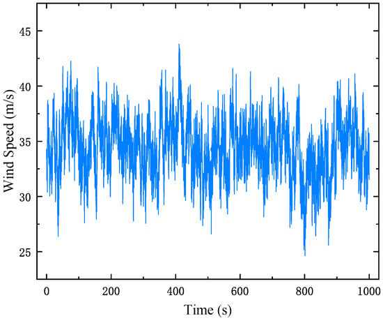
Figure 1.
Wind velocity time history.
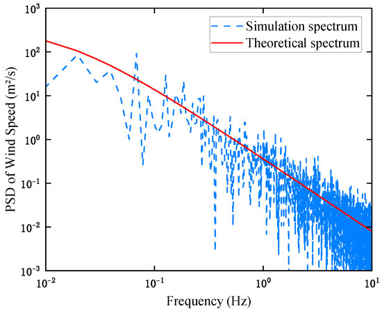
Figure 2.
Power spectrum comparison plot.
2.2. Rain Pressure Model
As a raindrop with diameter D descends, the horizontal and vertical rain pressures and can be defined as follows [38]:
In the equation, represents the density of the raindrop, taken as 1000 kg/m³, while and represent the instantaneous velocity components along the horizontal and vertical axes, respectively; denotes the velocity ratio [19]; represents the integral of the normalized curve from 0 to ; and denotes the number of raindrops within a given volume unit, while describes the raindrop size distribution raindrop spectrum, where indicates the slope factor and I represents the rainfall rate in mm/h.
2.3. Wind and Rain Load Impacts on the Tower–Line System
2.3.1. Wind and Rain Loading Effects on Lines
The wind force exerted on the lines is determined using the following formula:
In the equation, represents the force exerted by the wind on the transmission conductors and grounding cables; represents the wind pressure’s non-uniformity factor, set at 0.61; denotes the coefficient for height-dependent variation in wind pressure, taken as 1.0, and represents the shape factor for cables and grounding wires, with a value of 1.1; and d denotes the external diameter of the conductors and ground wires, represents the horizontal distance between the towers, and specifies the wind direction angle.
Due to the extensive length of transmission lines, the rain load is separated into horizontal and vertical components. The rain force exerted on the transmission lines is calculated using the equations provided below:
2.3.2. Wind and Rain Loading Effects on Towers
The wind force exerted on the tower is calculated based on the following equation:
In this formula, represents the wind stress exerted on the tower, denotes the tower’s shape coefficient, refers to the area of the tower’s surface exposed to the wind, and is the wind load adjustment factor, set to 1.0.
Owing to the design characteristics of towers, the area exposed to rain in the vertical direction is minimal. Therefore, only the horizontal component of the rain load is considered. However, raindrop impacts affect both sides of the tower in the horizontal plane. The rainfall force exerted on the tower is computed according to the equation below:
2.3.3. Wind and Rain Load Scenarios for Tower–Line Systems
The wind pressure exerted on the wires is decomposed into components in the x and y directions, denoted as and , respectively. For the tower body, wind forces are distributed across the “a” and “b” faces, represented by and , as illustrated in Figure 3. This figure visualizes the loading mechanisms on the “a” and “b” faces of the tower and the wires, offering a visualization of the loading mechanisms. These forces, which vary with the wind direction angle (), are calculated using standard design formulas [34]. Table 1 presents a comprehensive breakdown of the force components exerted by the wind on both the wires and the tower structure under different wind conditions.
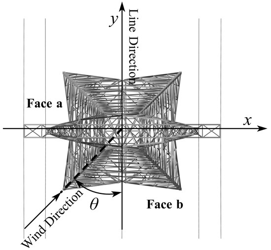
Figure 3.
Schematic diagram of wind direction angles.

Table 1.
Wind load components on wires and tower body under various wind directions.
This table presents a comprehensive breakdown of wind load components (, , , ) acting on the wires and tower body for various wind direction angles ().
Rainfall is considered an additional load working in conjunction with wind forces to excite the structure. Rather than being treated as an independent force, the rain-induced loads are combined with the wind loads, representing a coupled excitation acting on the wires and tower body.
2.4. Tower–Line System Dynamic Behavior Under Wind and Rain Forces
In this study, a real-world overhead transmission line project is chosen as the research subject. The system comprises two tower types: tension and suspension towers. A straight tension section without angle changes is selected for analysis, with Towers 1 and 3 as tension towers and Tower 2 as a suspension tower. The geometric configuration, including the positions of the towers, spans, and line heights, is illustrated in Figure 4, offering a comprehensive overview of the system.
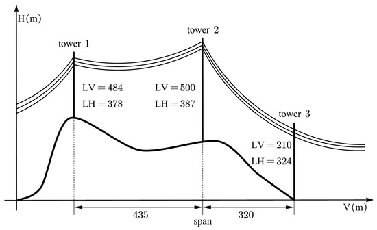
Figure 4.
Tower position diagram.
The tension tower has a total elevation of 39.50 m and a base size of 10.56 m, while the suspension tower measures 45.20 m in height and has a base width of 6.976 m. A detailed representation of the towers’ geometric design, including their dimensions and structural layouts, is shown in Figure 5. The transmission towers use Q345 equal-angle steel as the primary material, with Q235 equal-angle steel serving as the auxiliary material. Detailed cross-sectional properties of the sub-members, classified by tower sections and their components (e.g., ground wire support, cross arms, tower body, and legs), are presented in Table 2 and Table 3, which include the geometric properties of each sub-member.
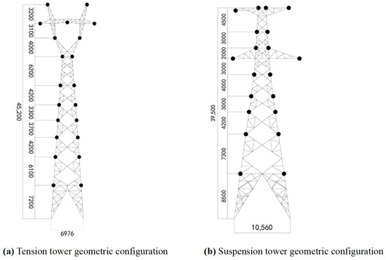
Figure 5.
Tower geometry diagram.
Table 2.
Tension tower parameters.
Table 3.
Suspension tower parameters.
Table 4 displays an overview for the properties of the tower components. A bilinear isotropic hardening model is utilized to account for material nonlinearity. The transmission conductor is specified as type JL/G1A-240/40, and the ground wire is type GJX-80, with their respective physical properties being listed in Table 5. The finite element model is constructed using ANSYS software, employing BEAM188 elements to simulate the structural members (angle steels) with precision in geometry and material characteristics. Connections between the steel bars in the towers are modeled with shared nodes, ensuring displacement and rotational continuity, effectively representing bolted or welded joints typically found in transmission tower structures. The tower legs are fixed to the concrete foundation, restricting all movement and rotation at the base nodes. This configuration reflects real-world boundary conditions by allowing the foundation to transfer forces and moments from the tower to the ground, ensuring overall structural stability. Link8 elements are used to represent insulators, which only carry tension, while Cable280 elements are used to represent the transmission lines and grounding cables, reflecting their tension-dominated, cable-like behavior. Support constraints are applied at the terminals of the conductors and grounding wires in the final span to improve stability. Figure 6 shows the complete finite element representation of the tower–line system.
Table 4.
Bilinear isotropic hardening model parameters for equal-angle steel.
Table 5.
Conductor and ground wire parameters.
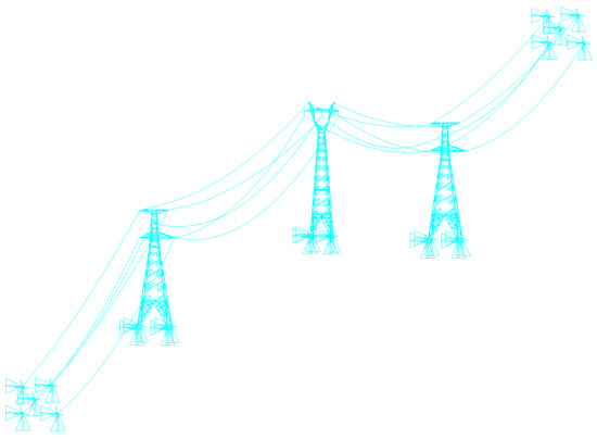
Figure 6.
Tower–Line system finite element model.
The tower and conductors are categorized into specific wind-exposed sections based on their structural configuration. The wind force applied to each section is represented as a concentrated load to enhance computational efficiency while maintaining the accuracy of the load distribution. The spatially discretized loading points for the wind and rain forces are depicted in Figure 7. The maximum displacement dynamic history of the tower and the maximum tension dynamic history of the line are illustrated in Figure 8a and Figure 8b, respectively.
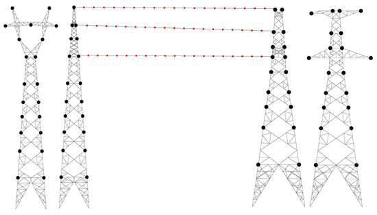
Figure 7.
Wind and rain load application points.
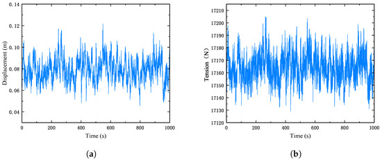
Figure 8.
Tower–Line system response. (a) Top displacement time history of the transmission tower; (b) maximum tension time history of the transmission line.
3. Surrogate Model Methodology
In summary, the surrogate model takes the time series of wind velocity and rainfall intensity as inputs, with the displacement at the tower’s peak and the maximum tension in the line serving as the outputs. A surrogate model built on TimesNet is employed to predict how the tower–line system behaves under the combined effects of wind and rain. The structure of the model implemented in this study is presented in Figure 9.
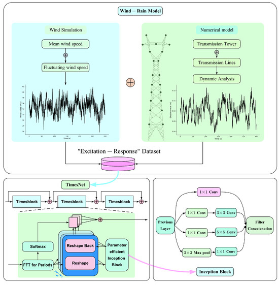
Figure 9.
Surrogate model framework.
3.1. Response Prediction Surrogate Model Based on TimesNet
TimesNet is a deep learning model specifically tailored to capture the complex periodic characteristics inherent in time series data. This is accomplished by using The fast Fourier transform to shift time-based data into the frequency domain, which allows for the identification of key periodic patterns. Using the extracted periodic information, the model reshapes the time series data into a 2D format, facilitating the capture of intricate temporal dependencies [31]. TimesNet is structured with stacked TimesBlock modules, connected via residual links to enhance feature propagation. The structure of TimesNet is illustrated in Figure 10. The input to the j-th TimesBlock is represented as , and the process is mathematically described as follows:
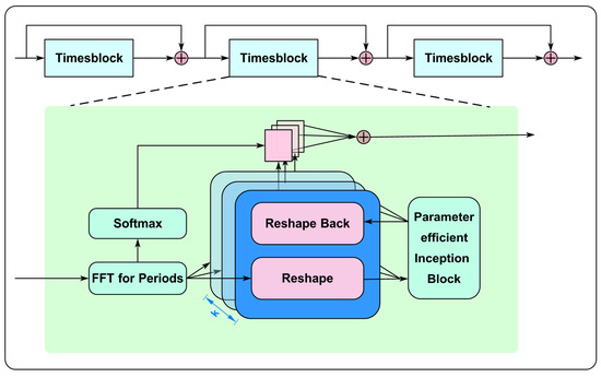
Figure 10.
Structure of TimesNet.
In the TimesBlock module, the original 1D wind and rain time series data are first transformed using FFT to shift from the time space to the frequency space. The frequency spectrum data are then applied to transform the original 1D temporal data into a 2D tensor format. The mathematical expression for this transformation process is given below:
In this equation, the time series data undergo a conversion from the time-based domain to the frequency-based domain through the use of . Here, denotes the computation of amplitude values. denotes the process of averaging the strength of each component across N-dimensions, resulting in A ∈ T. From this, the k components with the highest strength, denoted as , are extracted along with their corresponding periodic lengths . This process effectively identifies and preserves the most significant periodic features within the time series, laying a foundation for subsequent analysis.
Through the above process, k significant periodic lengths are obtained. Based on these periodic lengths, the raw 1D time series is folded accordingly. This method can be mathematically expressed as shown below:
To ensure that the time series length is divisible by the periodic parameter , the 1D time series is extended by appending zeros at the end using the function. Here, and represent the row and column dimensions of the reshaped 2D tensor.
Through this procedure, after converting the raw 1D time data into a 2D tensor, the TimesBlock employs the Inception block structure to extract feature representations from the tensor. The Inception block captures multi-scale features by utilizing convolution kernels of varying sizes within a single module while also reducing computational complexity. The design of the Inception block is depicted in Figure 11. This module effectively captures both the temporal features within individual segments of the time series and the relationships between different time periods, demonstrating its capacity to model the periodic characteristics of the data in depth. This process is mathematically expressed as:
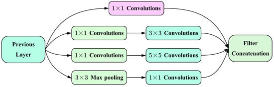
Figure 11.
Structure of the Inception block.
To enable the adaptive aggregation of multi-dimensional features in subsequent steps, the features obtained through the above equation are projected back into a one-dimensional space. This process is represented mathematically as:
The function eliminates the padded zeros introduced in Equation (23).
The significance of the chosen frequencies and periods is determined by the amplitude A obtained from the previous equation, which demonstrates the significance of each converted 2D tensor. Using the derived weight information, the k different 1D features are aggregated for further processing in the subsequent layer. This process is expressed as:
By utilizing variations within periods and across periods within the rows and columns of the two-dimensional tensor, the TimesBlock module effectively captures multi-scale temporal features in a two-dimensional framework. This approach allows TimesNet to extract features more efficiently compared with directly processing one-dimensional time series data.
3.2. Deep Learning-Based Surrogate Model for Time Series Prediction
As the current behavior of the tower–line system is impacted by its prior states, the structural dynamics demonstrate temporal dependencies. Therefore, it is logical to use a wind velocity time series with a time interval of T to forecast the corresponding response time series over the same interval T.
For a given set of excitation inputs v, a corresponding set of structural displacement response outputs x is obtained. The excitation time series is expressed as , while the structural response time series is represented by . Together, the input v and response x form structural “excitation–response” pairs, and multiple such pairs make up the input–output dataset used by the surrogate model. In this study, wind velocity and rain pressure are utilized for predicting the structural response. As a result, the final layer of the surrogate model is set up as a regression layer, with the mean squared error (MSE) serving as the loss function:
In the equation, represents the true value, signifies the predicted value, and n is the total number of predictions.
4. Experimental Results and Analysis
In this study, the data used for the surrogate model were created using a finite element numerical model. The dataset was distributed with 60% allocated to training, 20% to validation, and 20% to testing. All experiments were conducted on a system featuring an Intel Core i7-13700K processor, an NVIDIA GeForce RTX 4090 graphics card, and 32 GB of RAM.
4.1. Evaluation Metrics for Surrogate Model Performance
The surrogate model is devised to forecast the peak displacement of the tower and the highest tension in the lines, effectively capturing the time-varying response of the tower–line system affected by wind and rainfall forces. To measure the performance of the model’s predictions, three standard regression metrics are utilized: mean squared error (MSE), mean absolute error (MAE), and the coefficient of determination ():
4.2. Hyperparameters of Surrogate Model
The surrogate model includes several modules and parameters, each significantly influencing its prediction accuracy. The hyperparameters associated with the model are detailed in the Table 6:
Table 6.
Hyperparameters of the surrogate model.
In the Table 6, Batchsize indicates how many samples the model processes during each iteration. Dropout randomly deactivates certain neurons and their connections with a probability of 0.1 during training to minimize the risk of overfitting. indicates the number of TimesBlock modules included in the model. represents the size of the embedding layer in the model. indicates the size of the model’s fully connected layer. refers to the selection of the top k frequencies with the highest amplitude values. Each hyperparameter was carefully selected to optimize both training efficiency and prediction accuracy. To optimize the surrogate model, The Adam optimizer was used, starting with a learning rate of 0.0001. To ensure stable convergence, an exponential decay strategy was implemented, progressively reducing the learning rate during training. To avoid overfitting, an early stopping criterion was applied, which halts the training if the validation loss shows no substantial improvement over three consecutive epochs. This approach ensures a trade-off between model generalization and computational efficiency.
4.3. Effect of Window Size and Wind Direction Angle on Surrogate Model Performance
The time series data, comprising wind–rain load excitations and structural responses, are divided into equal-sized time windows during preprocessing. The window size affects the information density of the training data, which subsequently impacts the model’s performance. Therefore, this study evaluates five different window sizes: 10, 30, 50, 80, and 100.
To measure the prediction accuracy of the surrogate model under different wind direction angles, this study evaluates the most critical cases: 0°, 45°, 60°, and 90°. The baseline value for wind velocity is 27 m/s, with the rainfall intensity being maintained at 20 mm/h. Figure 12 illustrates the model’s predictive performance across different window sizes under these wind direction angles.
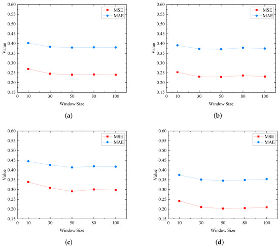
Figure 12.
Predictive performance of the surrogate model for different window sizes under various wind direction angles. (a) MSE and MAE for different window sizes at a 0° wind direction angle; (b) MSE and MAE for different window sizes at a 45° wind direction angle; (c) MSE and MAE for different window sizes at a 60° wind direction angle; (d) MSE and MAE for different window sizes at a 90° wind direction angle.
From the experimental findings in this research, the following conclusions can be made for various wind direction angles:
- When the window size is 10, both MSE and MAE reach their maximum values. As the window size increases, MSE and MAE gradually decrease, reaching their minimum values when the window size is 100. Therefore, a window size of 100 is recommended;
- The surrogate model demonstrates high predictive accuracy. For a 90° angle of wind direction, MSE is the smallest, at 0.2093, while for a 60° wind direction angle, the MSE is the largest, at 0.2997;
- As the window size increases, the accuracy of the surrogate model’s predictions improves, suggesting that the model is able to capture additional features. This outcome confirms the effectiveness of the surrogate model.
4.4. Performance Analysis of the Surrogate Model Prediction
In the previous section, we examined the effect of window size on the surrogate model’s prediction performance and determined that a window size of 100 yields the best results. The dataset utilized in this study consists of 20,000 samples, with input data comprising simulated wind velocity and rain pressure at monitoring points and outputs corresponding to the maximum displacement and tension in the system.
This section compares various models for predicting the dynamic behavior of the tower–line system, further evaluating the performance of the proposed surrogate model. All comparison algorithms, along with the surrogate model, were trained, validated, and tested using the same dataset and consistent preprocessing methods. The findings from these experiments are presented in Table 7.
Table 7.
Predictive performance of different models under various wind direction angles.
By analyzing the MSE, MAE, and metrics between actual and predicted values, the following conclusions are drawn: The 1D CNN model produces smaller prediction errors compared with the LSTM model, while the combined CNN-LSTM hybrid model further enhances prediction accuracy. It is noteworthy that the TimesNet-based surrogate model consistently surpasses the CNN, LSTM, and CNN-LSTM models for all wind direction angles. Specifically, the surrogate model reduces the MSE by an average of 27.6% compared with the CNN model, 29.4% compared with the LSTM model, and 26.1% compared with the CNN-LSTM model. Similarly, the MAE is reduced by an average of 18.6%, 20.3%, and 18.1%, respectively, while the metric improves by an average of 15.8%, 16.5%, and 15.4%, respectively. These findings show that the surrogate model maintains high prediction accuracy under different wind directions, even when considering the joint effects of wind and rain loads and the internal interactions within the tower–line system. Moreover, the results highlight the advantage of the TimesNet surrogate model, which leverages 2D CNN convolution to capture more intricate features compared with the 1D CNN convolution, significantly enhancing its accuracy and reliability. As illustrated in Figure 13a–c, the line charts for MSE, MAE, and metrics provide a clear comparison, underscoring the effectiveness of the TimesNet model across various wind direction angles.
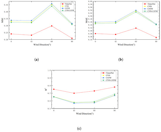
Figure 13.
Performance comparison of different models across various wind direction angles. (a) MSE comparison for different wind direction angles; (b) MAE comparison for different wind direction angles; (c) comparison for different wind direction angles.
4.5. Generalization Performance of the Surrogate Model
Assessments were performed to assess the generalization capabilities of the proposed TimesNet model and its predictive performance under various representative weather conditions. These scenarios were designed to encompass a wide variety of situations that transmission tower–line systems might encounter in real-world environments. Specifically, three wind velocities (20 m/s, 27 m/s, and 35 m/s) and three rainfall intensities (20 mm/h, 80 mm/h, and 120 mm/h) were selected, resulting in nine distinct weather combinations. This parameter set was carefully chosen to ensure a comprehensive evaluation of the model’s robustness and applicability.
The selected wind velocities correspond to moderate, strong, and extreme wind conditions. For example, 20 m/s represents typical strong wind scenarios, 27 m/s aligns with the design wind velocity of the analyzed tower–line system, and 35 m/s reflects extreme weather events, such as severe typhoons. Similarly, rainfall levels of 20 mm/h, 80 mm/h, and 120 mm/h correspond to moderate, heavy, and extreme rainfall conditions, respectively. By combining these wind velocities and rainfall intensities, nine unique weather scenarios were created. These scenarios, outlined in Table 8, comprehensively capture the behavior of the tower–line system under various environmental conditions, conducting a thorough examination of the model’s generalization performance.
Table 8.
Weather conditions.
In Section 4.3, we assessed how window size influences the capability of the surrogate model. In light of the experimental results, a window size of 100 was identified as optimal for achieving the best model performance and was therefore adopted for subsequent generalization experiments. Following the methodology outlined in Chapter 2, dynamic response samples of the tower–line system, impacted by the forces of wind and rain, were generated for nine distinct weather scenarios. Each sample consisted of 20,000 data points spanning a duration of 1000 s. The data were divided into training, validation, and testing sets with a 6:2:2 distribution. The final experimental outcomes are presented in Table 9.
Table 9.
Prediction performance of the surrogate model under different weather conditions.
The outcomes of the generalization experiments show that the proposed TimesNet model demonstrates strong predictive capabilities across different weather scenarios. By averaging the performance metrics across all nine scenarios, the model obtained an MSE value of 0.2542, an MAE value of 0.3895, and an score of 0.7214. These findings confirm that the TimesNet model consistently provides high prediction accuracy and reliability, highlighting its effectiveness in modeling the time-varying responses of tower–line systems.
5. Conclusions
This study presented a TimesNet-based surrogate model developed to forecast the dynamic behavior of tower–line systems affected by wind and rain forces. The research findings are summarized as follows: First, the model achieved optimal performance with a prediction window size of 100, attaining the lowest MSE and MAE, which demonstrates its ability to effectively capture temporal patterns and minimize prediction errors. Second, in generalization performance experiments conducted across nine weather scenarios (combining three wind velocities with three precipitation intensities), the model achieved an average MSE of 0.2542, an average MAE of 0.3895, and an average of 0.7214. These outcomes confirm the model’s robustness and reliability in predicting the system’s dynamic behavior under various weather conditions. Third, comparative experiments revealed that the TimesNet model outperformed the 1D CNN, LSTM, and CNN-LSTM models, with MSE being reduced by 27.6–29.4%, MAE being reduced by 18.1–20.3%, and being improved by 15.4–16.5%. These findings highlight TimesNet’s ability, leveraging its 2D convolution architecture, to capture complex temporal features and significantly improve predictive accuracy.
Moreover, the model requires only wind velocity and rainfall intensity to predict the system’s dynamic response with high accuracy, providing effective support for real-time health monitoring of transmission tower–line systems. A computational cost analysis reveals that the proposed TimesNet model has 1.18 million trainable parameters, achieving an average inference time of approximately 9 milliseconds per batch (batch size = 32) on an NVIDIA RTX 4090 GPU. These findings indicate that the model is lightweight and highly efficient, making it well suited for real-time applications. Additionally, by incorporating meteorological forecast data, the model can evaluate the system’s future response state, offering a robust scientific basis for disaster prevention and early warning strategies.
Given the limitations of existing methods and technologies, it is challenging for the dataset to encompass all potential wind velocity and rainfall intensities. To address this, this study selected nine representative weather scenarios. The findings show that the proposed surrogate model accurately predicts the dynamic behavior of the tower–line system under challenging environmental conditions. Furthermore, to explore the interactions between wind and rain loads, reasonable assumptions were made regarding their coupling effects. While these assumptions may simplify the coupling dynamics, they were designed to enhance computational efficiency without compromising theoretical rigor. These assumptions are consistent with current theories and align with existing research findings. Future work could explore extending the TimesNet model to other structural health monitoring scenarios, such as real-time monitoring and early warning for bridges, buildings, or critical infrastructure under complex loading conditions. Such efforts would not only validate the model’s adaptability but also expand its application in structural engineering.
Author Contributions
Conceptualization, Y.L. (Yingna Li) and B.Y.; methodology, Y.L. (Yifan Luo) and B.Y.; software, Y.L. (Yifan Luo); validation, Y.L. (Yifan Luo); formal analysis, Y.L. (Yingna Li); Y.L. (Yifan Luo) and BY.; investigation, B.Y.; resources, Y.L. (Yingna Li) and B.Y.; data curation, Y.L. (Yifan Luo); writing—original draft preparation, Y.L. (Yifan Luo); writing—review and editing, Y.L. (Yingna Li), B.Y., L.W. and Y.L. (Yifan Luo); visualization, L.W., Y.L. (Yifan Luo) and J.Z.; supervision, Y.L. (Yingna Li) and B.Y.; project administration, Y.L. (Yingna Li) and B.Y.; funding acquisition, Y.L. (Yingna Li). All authors have read and agreed to the published version of the manuscript.
Funding
This research was funded by the Key projects of science and technology plan of Yunnan Provincial Department of Science and Technology (grant number 202201AS070029).
Data Availability Statement
The data that support the findings of this study are available from the author, Yifan Luo, upon reasonable request.
Conflicts of Interest
The authors declare no conflict of interest.
References
- He, B.; Zhao, M.; Feng, W.; Xiu, Y.; Wang, Y.; Feng, L.; Qin, Y.; Wang, C. A method for analyzing stability of tower-line system under strong winds. Adv. Eng. Softw. 2019, 127, 1–7. [Google Scholar] [CrossRef]
- Bi, W.; Tian, L.; Li, C.; Ma, Z. A Kriging-based probabilistic framework for multi-hazard performance assessment of transmission tower-line systems under coupled wind and rain loads. Reliab. Eng. Syst. Saf. 2023, 240, 109615. [Google Scholar] [CrossRef]
- Rong, W.; Wang, Z.; Jiang, W.; Xu, F.; Duan, Z.; Ou, J.P. CFD Numerical Simulation of Wind and Rain Load Characteristics on Transmission Towers. J. Disaster Prev. Mitig. Eng. 2024, 44, 1115–1125. [Google Scholar]
- Fu, X.; Li, H.; Li, G.; Xu, X. Advances in calculation theory of wind and rain loads and failure estimation for transmission tower-line systems. J. Build. Struct. 2023, 44, 198–212. [Google Scholar]
- Moschas, F.; Stiros, S. High accuracy measurement of deflections of an electricity transmission line tower. Eng. Struct. 2014, 80, 418–425. [Google Scholar] [CrossRef]
- Zhang, X.; Zhao, Y.; Zhou, L.; Zhao, J.; Dong, W.; Zhang, M.; Lv, X. Transmission tower tilt monitoring system using low-power wide-area network technology. IEEE Sens. J. 2020, 21, 1100–1107. [Google Scholar] [CrossRef]
- Bian, R.; Xu, Q.; Yu, E.; Huang, M.; Lou, W.; Hu, W.; Zhang, L. Multi-variate state monitoring and wind bias reliability analysis of a transmission tower-line system under action of typhoon. J. Vib. Shock 2020, 39, 52–59. [Google Scholar]
- Takeuchi, M.; Maeda, J.; Ishida, N. Aerodynamic damping properties of two transmission towers estimated by combining several identification methods. J. Wind Eng. Ind. Aerodyn. 2010, 98, 872–880. [Google Scholar] [CrossRef]
- Szafran, J.; Rykaluk, K. A full-scale experiment of a lattice telecommunication tower under breaking load. J. Constr. Steel Res. 2016, 120, 160–175. [Google Scholar] [CrossRef]
- Tian, L.; Pan, H.; Ma, R.; Zhang, L.; Liu, Z. Full-scale test and numerical failure analysis of a latticed steel tubular transmission tower. Eng. Struct. 2020, 208, 109919. [Google Scholar] [CrossRef]
- Lou, W.; Sun, B. Wind-Structure-Conpling effects and buffeting responses. Eng. Mech. 2000, 17, 16–22. [Google Scholar]
- Xie, Q.; Cai, Y.; Xue, S. Wind-induced vibration of UHV transmission tower line system: Wind tunnel test on aero-elastic model. J. Wind Eng. Ind. Aerodyn. 2017, 171, 219–229. [Google Scholar] [CrossRef]
- Liang, S.; Zou, L.; Wang, D.; Cao, H. Investigation on wind tunnel tests of a full aeroelastic model of electrical transmission tower-line system. Eng. Struct. 2015, 85, 63–72. [Google Scholar] [CrossRef]
- Huang, M.; Lou, W.; Yang, L.; Sun, B.; Shen, G.; Tse, K. Experimental and computational simulation for wind effects on the Zhoushan transmission towers. Struct. Infrastruct. Eng. 2012, 8, 781–799. [Google Scholar] [CrossRef]
- Haifeng, B. The Dynamic Response of Transmission Tower-Line System Sbujected to Environmental Loads. Ph.D. Thesis, Dalian University of Technology, Dalian, China, 2007. [Google Scholar]
- Battista, R.C.; Rodrigues, R.S.; Pfeil, M.S. Dynamic behavior and stability of transmission line towers under wind forces. J. Wind Eng. Ind. Aerodyn. 2003, 91, 1051–1067. [Google Scholar] [CrossRef]
- Felchak, L.; Fernandes, J.; Mendonça, J.; Dos Santos, A.; Jarek, A.; Tonetti, M.; De Lacerda, L.; Penteado, R. Numerical analysis of insulated and conventional cross arms for transmission line tower. Eng. Struct. 2023, 294, 116710. [Google Scholar] [CrossRef]
- Fu, X.; Li, H.N.; Li, G.; Dong, Z.Q. Fragility analysis of a transmission tower under combined wind and rain loads. J. Wind Eng. Ind. Aerodyn. 2020, 199, 104098. [Google Scholar] [CrossRef]
- Fu, X.; Li, H.N.; Li, G. Fragility analysis and estimation of collapse status for transmission tower subjected to wind and rain loads. Struct. Saf. 2016, 58, 1–10. [Google Scholar] [CrossRef]
- Dadras Eslamlou, A.; Huang, S. Artificial-neural-network-based surrogate models for structural health monitoring of civil structures: A literature review. Buildings 2022, 12, 2067. [Google Scholar] [CrossRef]
- Flah, M.; Nunez, I.; Ben Chaabene, W.; Nehdi, M.L. Machine learning algorithms in civil structural health monitoring: A systematic review. Arch. Comput. Methods Eng. 2021, 28, 2621–2643. [Google Scholar] [CrossRef]
- Silionis, N.E.; Liangou, T.; Anyfantis, K.N. Deep learning-based surrogate models for spatial field solution reconstruction and uncertainty quantification in Structural Health Monitoring applications. Comput. Struct. 2024, 301, 107462. [Google Scholar] [CrossRef]
- Li, T.; Pan, Y.; Tong, K.; Ventura, C.E.; de Silva, C.W. Attention-based sequence-to-sequence learning for online structural response forecasting under seismic excitation. IEEE Trans. Syst. Man Cybern. Syst. 2021, 52, 2184–2200. [Google Scholar] [CrossRef]
- Xiang, P.; Zhang, P.; Zhao, H.; Shao, Z.; Jiang, L. Seismic response prediction of a train-bridge coupled system based on a LSTM neural network. Mech. Based Des. Struct. Mach. 2024, 52, 5673–5695. [Google Scholar] [CrossRef]
- Liao, Y.; Lin, R.; Zhang, R.; Wu, G. Attention-based LSTM (AttLSTM) neural network for seismic response modeling of bridges. Comput. Struct. 2023, 275, 106915. [Google Scholar] [CrossRef]
- Zhang, Z.; Liu, X.; Wang, Y.; Li, E.; Zhang, Y. Stability Prediction Model of Transmission Tower Slope Based on ISCSO-SVM. Electronics 2024, 14, 126. [Google Scholar] [CrossRef]
- Xue, J.; Xiang, Z.; Ou, G. Predicting single freestanding transmission tower time history response during complex wind input through a convolutional neural network based surrogate model. Eng. Struct. 2021, 233, 111859. [Google Scholar] [CrossRef]
- Zhu, X.; Ou, G.; Pu, Z.; Li, X.; Xue, J. In-event surrogate model training for regional transmission tower-line system dynamic responses prediction in realistic hurricane wind fields. Struct. Infrastruct. Eng. 2024, 1–21. [Google Scholar] [CrossRef]
- Fayaz, J.; Galasso, C. A deep neural network framework for real-time on-site estimation of acceleration response spectra of seismic ground motions. Comput.-Aided Civ. Infrastruct. Eng. 2023, 38, 87–103. [Google Scholar] [CrossRef]
- Peng, H.; Yan, J.; Yu, Y.; Luo, Y. Time series estimation based on deep learning for structural dynamic nonlinear prediction. Structures 2021, 29, 1016–1031. [Google Scholar] [CrossRef]
- Wu, H.; Hu, T.; Liu, Y.; Zhou, H.; Wang, J.; Long, M. Timesnet: Temporal 2d-variation modeling for general time series analysis. In Proceedings of the 2023 11th International Conference on LeFarning Representations, Kigali, Rwanda, 1–5 May 2023. [Google Scholar]
- Yang, M.; Han, C.; Zhang, W.; Wang, B. A short-term power prediction method for wind farm cluster based on the fusion of multi-source spatiotemporal feature information. Energy 2024, 294, 130770. [Google Scholar] [CrossRef]
- Wei, H.; Chen, Y.; Yu, M.; Ban, G.; Xiong, Z.; Su, J.; Zhuo, Y.; Hu, J. Alleviating distribution shift and mining hidden temporal variations for ultra-short-term wind power forecasting. Energy 2024, 290, 130077. [Google Scholar] [CrossRef]
- DL/T5154-2012; Technical Code for the Design of Tower and Pole Structures of Overhead Transmission Line. China Planning Press Beijing: Beijing, China, 2012.
- ASCE-No.74; Guidelines for Electrical Transmission Line Structural Loading. American Society of Civil Engineers: Reston, VA, USA, 2009.
- Kaimal, J.C.; Wyngaard, J.; Izumi, Y.; Coté, O. Spectral characteristics of surface-layer turbulence. Q. J. R. Meteorol. Soc. 1972, 98, 563–589. [Google Scholar]
- Zhitao, Y. Study on Wind-Induced Vibration of Long Span Half-Through Arch Bridges. Ph.D. Thesis, Chongqing University, Chongqing, China, 2006. [Google Scholar]
- Wang, Z.; Xiang, Y.; Wang, T. Assessment Method of Tower Falling and Line Disconnection Accidents for 110 kV Line in Typhoon andTorrential Rain Disaster. Autom. Electr. Power Syst. 2022, 46, 59–66. [Google Scholar]
Disclaimer/Publisher’s Note: The statements, opinions and data contained in all publications are solely those of the individual author(s) and contributor(s) and not of MDPI and/or the editor(s). MDPI and/or the editor(s) disclaim responsibility for any injury to people or property resulting from any ideas, methods, instructions or products referred to in the content. |
© 2025 by the authors. Licensee MDPI, Basel, Switzerland. This article is an open access article distributed under the terms and conditions of the Creative Commons Attribution (CC BY) license (https://creativecommons.org/licenses/by/4.0/).