Abstract
Modern AMSs (automated manufacturing systems) on the one hand bring many benefits, but on the other hand, they are cumbersome to coordinate. AMSs consist of various subsystems (e.g., production lines) that share a finite number of resources (robots, machines, buffers, automated guided vehicles, etc.). This forces AMS designers to build flexible and decentralized systems. However, in these cases, the danger of deadlocks exists. Consequently, such a situation requires the application of advanced supervisors. One solution to the deadline problem is the application of Petri nets. This paper is motivated by AMS control based on deadlock prevention by means of ordinary Petri nets (OPNs) and generalized Petri nets (GPNs). This paper examines two areas of AMS Petri net-based model structures and presents methods of deadlock prevention. First, simpler structures of AMSs modeled by OPNs and GPNs will be investigated, and then more complex structures of AMSs modeled by the same kinds of Petri nets (PNs) will be analyzed. The siphon-based approach will be used for deadlock prevention in all of these cases. The principal results are introduced, explained, and illustrated through examples. Key results are introduced, especially in Example 1 and Example 2.
1. Introduction
Automated manufacturing systems (AMSs), often called flexible manufacturing systems (FMSs), are systems consisting of a set of production robotic cells and lines capable of automatically producing a variety of piece types (parts) simultaneously. They are discrete-event systems (DESs) and are controlled by computers. AMSs pose a high degree of automation, integration, and flexibility far beyond traditional forms of handling with raw materials and parts in manufacturing systems. Petri nets (PNs) are frequently used in modeling AMSs and in their supervisory control synthesis. It is useful when both the plant itself and its supervisor can be modeled by such a uniform formalism.
This research area dates back more than four decades. A very important part of this research is the problem of allocation of resources. Resource allocation systems (RASs) with shared resources contain many proposed methodologies. Practically all of the papers referred here, except [1,2], use siphons for deadlock prevention. These two articles deal with reachability graphs and graphs in general, respectively.
There are many subclasses of PN models in the literature—see, e.g., Table 1 in [3], where 27 subclasses are presented with their full names and shortcuts, and it is also stated there whether a given subclass belongs to ordinary or generalized Petri nets.
It is necessary to mention Systems of Simple Sequential Processes with Resources (PR) and Extended PR (PR), which are both used very frequently. In addition, Systems of Simple Sequential Processes with General Resource Requirements () are used (e.g., in [4,5,6,7,8]), and a Generalized Linear System of Simple Sequential Processes with Resources (PR) is used in [9], which is a subclass of R [10,11]. The same class of resource acquisition behavior, named as the PR (Simple Systems of Simple Sequential Processes with Resources) net structure, was originally proposed in [12] and mentioned as well in [5], where strict minimal siphons are also further elaborated with the intent of avoiding the necessity to find all elementary siphons. Further works in the area of GPNs and PR include [5,6,9,10,13,14,15,16,17,18,19,20,21,22,23,24,25,26].
There are three principal strategies for dealing with deadlocks. (i) Deadlock detection and recovery [27,28,29,30,31,32] is usually used in cases where deadlocks are not so frequent and the consequences are not too serious. (ii) Deadlock prevention (see e.g., [4,9,10,15,16,17,18,19,20,26,31,33,34,35,36,37,38,39,40,41,42,43,44,45,46,47]) restricts interactions among resources and their users; requests for resources have to be prevented because they may lead to deadlocks. (iii) Deadlock avoidance ([11,15,28,31,36,48,49,50]) assigns a resource to a user only if the consequential state is not a deadlock. This paper examines only the deadlock prevention strategy.
This paper is a free continuation of the author’s previous paper [34]. Here, not only simple AMS models but also more complex AMS models, based on ordinary PNs (OPNs) and/or generalized PNs (GPNs), will be presented. The deadlock prevention strategy will be in all cases based on siphons. Siphons are [51] immediately related to deadlocks. Some authors in older studies, e.g., in [52,53], even identify siphons with deadlocks. Therefore, siphons are often utilized in the analysis and control of deadlocks. Any Petri net has a reachability tree/graph unambiguously that belongs to it. Hence, such a tree/graph is very suitable for verifying the deadlock’s absence. In this paper, no other quantitative metrics are utilized. Of course, there exist papers—see, e.g., [54,55]—where such research is performed. This paper is based on logical inconsistency measures. Observable PN liveness is analyzed in [56]. Some other papers devoted to deadlock detection are presented, e.g., in [57], where PN decomposition techniques are applied, such as in [58], and in [59,60], a transitive matrix of resource share places is used.
In order to verify the deadlock’s absence, reachability trees/graphs will be used in this paper.
1.1. Multisets
Multisets will be used to simplify the complexity of the problems. A more comprehensive definition of a multiset follows:
Definition 1
([33]). A multiset Ω, over a non-empty set A, is a mapping , which we represent as a formal sum . A multiset is a generalization of the concept of a set. In multiset Ω, non-negative integer is the coefficient of element , indicating the number of occurrences of a in Ω. It is said that belongs to Ω, which is denoted by , if . It does not belong to Ω, as denoted by , if . Let and be two multisets. The basic operations on multisets are union, intersection, addition, difference, and comparison, which are defined, respectively, as follows:
- ;
- ;
- ;
- ;
- ;
- .
Example of Applications
A few micro-examples are provided here to demonstrate what it is like working with multisets. Let , and be three multisets over . We have , , , , , , , , and . It can be said that multiset is less than if and is greater than or equal to if . A multiset without any element is denoted by ∅ (i.e., as an empty set). If the multiplicity of every element is one, a multiset becomes a set.
With respect to [14], a multiset , over a non-empty set D, is a mapping , which is denoted as a formal sum .
Here, represents the set of natural numbers plus zero.
1.2. Aim of the Paper
The main aim of this paper is to resolve situations related to AMS control when the capacity for resources is minimal. In the case of OPN models of AMSs, these are the situations when the marking of places representing resources are equal to one. In case of GPN models of AMSs, these are the situations when the marking of the place representing a resource is equal to the weight of the arc, which is greatest out of all of the weights of arcs directed to output transitions.
In such cases, it is not so much a matter of computational complexity as it is of finding a solution that exists when other approaches fail.
The subgoal is also to compare the results with those obtained using complementary siphons.
Example 1 demonstrates the case of an OPN model of an AMS with limited resources using siphons to prevent deadlocks, while Example 2 uses complementary siphons for the same case. By comparing the results in the form of reachability graphs, it was found that the results obtained in Example 1 for deadlock prevention are better than those obtained in Example 2.
As mentioned above, this paper is a free continuation of the paper [34], where a case of deadlock prevention of the PR model of an AMS was presented. Here, five examples are presented. Three of them—Examples 1, 2, and 4—concern PR kinds of OPN models, while the remaining two—Examples 3 and 5—concern PR kinds of GPN models.
1.3. Structure of the Article
In Section 2, basic knowledge about Petri nets is introduced. The conditions and constraints of the controllability of siphons are introduced in Section 3. Both OPN-based and GPN-based models of AMSs are analyzed. Definitions, lemmas, propositions and theorems concerning the siphon-based control are introduced here. All of them include references to the original literature. Procedures that ensure the parameters of supervisors and the deadlock-freeness are introduced here as well.
Section 4 is devoted to four illustrative examples (Examples 1–4) documenting the results of the supervisory control of particular paradigms of AMS models. Two categories of AMS models are introduced—models with a simpler structure based either on an OPN (Example 1 in Section 4.1 and Example 2 in Section 4.2) or on a GPN (Example 3 in Section 4.3) and the model with a more complex structure based on an OPN (Example 4 in Section 4.4). In Section 5, the approach to deadlock prevention in PR models of AMSs based on GPNs is presented and illustrated by Example 5 in Section 5.2.
2. Basics of Petri Nets
A short introduction to the Petri net topic was already made in [34]. However, it is necessary to introduce the basics of them here as well.
A Petri net is a quadruplet where P and T are finite non-empty sets; the set of places while the set of transition , whereby it is true that and ; ∅ means an empty set. The set expresses the flow relation in N. Flows consist of both directed arcs from the places to transitions and vice versa. The mapping assigns a weight to an arc: if and W(f) = 0 otherwise. Here, represents the set of natural numbers plus zero. The net N where , is the ordinary Petri net (OPN) . If , the net is the generalized net (GPN).
A transition without input places is called a source transition and a transition without output places is called a sink transition. Source transitions are always enabled, while the firing of a sink transition generates no tokens. Sink transitions are only consuming (devouring) tokens.
A place in N is marked at marking M if . A place is insufficiently marked with respect to a transition at M if . The symbol denotes the set of output transitions emerging from the place p. If at least one place in a subset is marked at M, then S is marked at M. denotes the sum of tokens in all places in S, i.e., . If , S is said to be empty at M. If , S is said to be insufficiently marked at M.
A subset is marked by M if and only if at least one place is marked by M. Thus, represents the sum of tokens in all places in D.
In general, is the preset of a node , while is the postset of a node .
Let a marked ordinary Petri net be . A transition t is enabled at M, expressed by , if . An enabled transition t at M can be fired. Consequently, a new marking arises. It may be denoted by , where , ; otherwise, .
A PN marking M is an vector. It is frequently called a state vector. The evolution of PN marking is performed by means of the following relationship:
where is an initial marking, is the incidence matrix, and is a vector of non-negative integers, which is called a firing vector. Elements of indicate the algebraic sum of all occurrences of t in . The set of all markings reachable from M by firing any possible sequence of transitions is denoted as . is the set of reachable markings of a Petri net starting from the initial marking .
Equation (1) constitutes the mathematical model of the Petri net N. The matrix is the incidence matrix. It presents the matrix form of the set F. It can also be written in the shape . Finally, is an vector expressing the firing of transitions. It can also be called the control vector because it represents the state of transitions. When a transition is enabled (i.e., able to be fired), the i-th element of the vector is indicated by 1. In the opposite case, when the transition is disabled, it is indicated by 0. It is important is to say that the enabled transition may or may not be fired. The marking of a place p is an integer indicating the number of tokens located in this place. The place p is marked by M if and only if .
A non-empty subset of places is a siphon if and only if . A non-empty subset of places is a trap if and only if . A siphon S is minimal if and only if there is no siphon contained in it as a proper subset. A minimal siphon S is said to be strict if . When a minimal siphon S does not contain a marked trap, it is called a strict minimal siphon (SMS). Such siphons have to be controlled in order to prevent their emptying.
Siphons are extensively used in a large amount of approaches concerning the deadlock control and liveness-enforcing for both OPN and GPN models of AMSs.
A siphon (trap) S (Q) is said to be empty at marking M if and only if ().
S or Q is said to be max-marked (min-marked) at a marking M if and only if or such that , where .
As to [61] and many other sources, P-invariant (place invariant) and T-invariant (transition invariant) are two weighty structural properties of PNs that are important in mathematical computations with PN models of AMSs.
It is necessary to emphasize that a P-vector is a column vector (indexed by P), where is the set of all integers. A P-vector I is called P-invariant if and . A P-invariant is minimal if and only if it contains no P-invariant as a proper subset. A P-invariant I is P-semiflow if every element of I is non-negative. is named the support of a P-invariant. It is defined as .
A T-vector is a column vector (indexed by T). A T-vector D is called T-invariant if and . The support of a T-invariant is defined as .
3. Siphon Controllability Conditions and Constraints
In the literature, there is a galaxy of articles that deal with the control of DESs, AMSs, and FMSs. A large number of them use Petri nets (PNs) of different kinds to model and control such systems. Some papers use an approach based on P-invariants of the PN model—see, e.g., [62], but many more papers use approaches based on PN siphons. Among these, the following are worthy of mention [5,7,8,13,35,38,41,42,43,44,45,57,62,63,64,65,66,67,68,69,70,71,72]. Some of the definitions, properties, lemmas and theorems used in this paper have been taken from other literature. For each such item, there is a corresponding reference to the authors. Also, some PhD theses are well known in this area—see, e.g., [49,73,74].
Here, in this section, particular classes of PN models will be analyzed: first, AMS models based on ordinary Petri nets (OPNs), being represented by means of PRs, and then those models based on generalized Petri nets (GPNs).
3.1. Systems of Simple Sequential Processes with Resources (PRs)
Definition 2
([40]). A System of Simple Sequential Processes with Resources (PR) is defined as a union of a set of nets sharing common places, where the following statements are true:
- 1.
- is called the process idle place of . Places from sets and are called operation and resource places, respectively.
- 2.
- (a) ;(b) ;(c) The two following statements are verified: (i) and (ii) ;(d) .
- 3.
- .
- 4.
- is a strongly connected state machine, where is the resultant net after the places in and related arcs are removed from .
- 5.
- Every circuit of contains place .
- 6.
- Any two s are composed when they are composables. Every shared place must be a resource.
More precise definitions of PRs utilizing concurrently PRs (Simple Sequential Processes with Resources) can be found in [17,75].
For each SMS in N (i.e., in the PN model of a plant), a monitor has to be added [17] in order to prevent it from emptying. By adding a sufficient amount of monitors (frequently called control places), the liveness of N is enforced in order to prevent siphons from emptying.
Definition 3
([17]). A siphon S is said to be controlled in a net system if and only if , .
In a deadlock structure, the set of transitions plays an important role. In accordance with [17], the set of resources used in output places of the transition set is equal to the set of resources used in the input places of the transition set. In such a situation, the system enters a deadlock state just at that moment if the number of resources that the deadlock structure uses is equal to the resource capacity. Therefore, the control policy consists of adding places, called monitors, that ensure that for each resource involved, the deadlock structure always requires fewer resources than the system actually has. Moreover, in such a case, the policy is minimally restrictive; that is, it is [17,47,76,77] optimal or maximally permissive.
Concisely said, the necessity of a supervisor arises from the fact that for each SMS in N, a monitor must be added to prevent it from emptying.
SMSs in Petri nets are either elementary or dependent. Dependent siphons are further divided into strongly and weakly dependent with respect to elementary siphons. It was proved [17] that the number of the elementary siphons is ; i.e., it is bounded by the smaller from the counts of places and transitions. In addition, a dependent siphon can be controlled by properly supervising the number of tokens in its elementary siphons.
In the literature, e.g., [78], two concepts are distinguished—bad state and dangerous state. In a bad marking, N will inevitably reach a deadlock. In a dangerous marking, the system may not reach a deadlock if the firings of enabled transitions are properly controlled by the supervisor. The policy of deadlock avoidance consists of ensuring that the system never reaches a bad state.
Monitors can only be added for elementary siphons. The controllability of a dependent siphon is ensured by properly supervising the initial number of tokens in the monitors. This means that it no longer needs to explicitly add a monitor for a dependent siphon.
3.1.1. Controllability of Elementary Siphons
Definition 4
([17]). Let be a subset of places of Petri net . P-vector S is called the characteristic P-vector of S if and only if ; otherwise, .
Definition 5
([17]). is called the characteristic T-vector of S, where is the transpose of incidence matrix .
Definition 6
([17]). Let be a net with and be a set of siphons of . Let be the characteristic -vector of siphon . and are called the characteristic P- and T-vector matrices of the siphons in N, respectively.
Definition 7
([17]). Let be a linearly independent maximal set of matrix . Then, is called a set of elementary siphons in N.
Definition 8
([17]). is called a strongly dependent siphon if , where .
Definition 9
([17]). is called a weakly dependent siphon if , such that , and , where .
Lemma 1
([17]). The number of elements in any set of elementary siphons in net N equals the rank of .
Theorem 1
([17]). .
With respect to [75], a siphon S is a set of places where tokens can leak out into another set of places called complementary set of the siphon. It means that tokens stay either in S or . Thus, S and together form the support of a P-invariant. So, the total number of tokens in S and is conservative.
Once a siphon capable of being emptied (i.e., emptiable siphon) is found, the output transitions of places included in it can never be fired. This implies that the net N is not live and includes deadlocks. To prevent a siphon S from emptying, a control place (monitor) and some control arcs are added so that together with form a part of the support of a new P-invariant. It means that with the help of controlling the initial number of tokens in , we can restrict the maximal number of tokens leaking from S into . Thus, it can be said that S is invariant-controlled.
Property 1
([75]). For a given SMS S in an PR N, is the support of a P-invariant of N.
Property 2
([17,75]). Let be a strict redundant (the newer term is strongly dependent in the sense of [79]) SMS with respect to elementary siphons , in an PR. We have .
Lemma 2
([75]). Let be an ordinary Petri net (PN) system, and let S be an SMS. Monitor with added to S such that and form the support of a new minimal P-invariant associated with S, where , and .
- 1.
- .
- 2.
- .
- 3.
- If S is never empty, then .
- 4.
- .
Hence, plus its holder set of places form the support of a new P-invariant.
Lemma 3
([75]). Let S be an SMS in a marked PR . Monitor with added to S such that and form the support of a new P-invariant. If siphon S is never empty, then .
Definition 10
([15]). Let be an PR and S be a strict minimal siphon in N, where , and . Let . is called the complementary set of siphon S.
In some studies, P is denoted as .
It was proved in [16] that for a siphon S in an PR which does not contain the support of a P-invariant, , also we have . Moreover, we have the following:
- and are the supports of P-invariants of the PR;
- Let be a strict minimal siphon in N, where . Then, and ;
- Given a strict minimal siphon S in N, is the support of a P-invariant of N.
Definition 11
([80]). Let be a siphon of N, is called the complementary vector of S if ; otherwise, .
3.1.2. Controllability for Strongly Dependent Siphons
The aim of deadlock prevention is to disturb the controller region the least [81]. Therefore, should be allowed to reach its maximum. Thus, setting , S is said to be limit controlled. In general, , where , is the control depth variable. If some dependent siphons are not controlled, is adjusted to be greater than 1. As a consequence, max is less than and the controller region is more disturbed. Due to this, the controller is losing more reachable states.
Definition 12
([81]). Let where is called the control depth variable. S is said to reach its limit state when ; it is limit-controlled if and only if it is able to reach its limit state but not able to reach unmarked state; i.e., or .
Theorem 2
([81]). Let be a net system and be a strongly dependent SMS with respect to elementary siphons such that where , and if and only if . is extended by n control places such that are limit-controlled. can never be emptied if and only if .
It means that for strongly dependent siphon is a single resource r. means that in the initial marking of r, there is only one token.
Definition 13
([82]). Let be a reliable resource place in an PR N. The operation places that use r are known as the set of holders of r, which are indicated by . is said to be the complementary set of S if .
3.1.3. Controllability for Weakly Dependent Siphons
Theorem 3
([17]). A weakly dependent siphon S is controlled if where and .
With respect to [51], a weakly dependent siphon S is max-controlled if , where .
Corollary 1
([17]). A weakly dependent siphon S is controlled if where and
3.2. Controllability of Siphons in GPN Models of AMSs
Definition 14
([14]). A siphon is said to be maximally (respectively, minimally) controlled if it is max-marked (respectively, min-marked) at any reachable marking.
When at least one place p in a siphon S contains enough tokens to fire any transition , S is called the max-marked siphon.
When at least one of places p of a siphon S contains enough tokens to fire at least one transition , S is called the min-marked siphon.
If a siphon is max-controlled, it is also min-controlled but not vice versa.
The following three formulations ensure the max cs-property of N.
Definition 15
([39,83]). A net is said to be satisfying the max cs-property (controlled-siphon property) if and only if each minimal siphon of N is max-controlled.
Lemma 4
([39,83]). If a net satisfies the max cs-property, it is deadlock-free.
Theorem 4
([36]). Let be a marked R net. N is live under if and only if it satisfies the max cs-property.
Consequently, invariant-controlled siphons represent a special case of max-controlled siphons.
Proposition 1
([83]). Let be a Petri net and S be a siphon of N. If there exists a P-invariant I such that , and , then S is max-controlled.
This concept of cs-property was utilized in [34] to solve a problem of deadlock prevention in the case of PR models of AMSs. Here, it will be used for PR models.
4. Examples of PN Models with a Simpler Structure
In this section, applications of the above introduced theory are introduced in the form of examples. In each of them, our partial contribution is submitted.
Here, the term simpler structure means a PN structure with a smaller number of places and transitions (the sharp boundary between smaller and larger numbers is not determined) and less complex structure of interconnections between places and transitions (however, there is no sharp definition here, either). Another factor is how the PN model behaves in different calculations. Therefore, this term is only intuitive.
Let us solve the following example utilizing Definitions 4–6 introduced in Section 3.1.1 as well as further definitions, properties, theorems and lemmas in Section 3.1.1 and Section 3.1.2.
4.1. Example 1
Consider the example of the PN model of an AMS displayed in Figure 1. The PR model of AMS (on the left) and its reachability tree (RT) are on the right. As we can see in RT, there are two discontinuities, namely, RT nodes 13 and 14 have no output arcs. It means that the PN states represented by them are deadlocks. Strict minimal siphons and traps are introduced in Table 1.
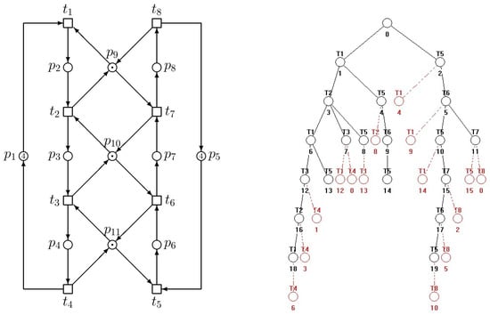
Figure 1.
An PR PN model of AMS (left) and its RT (right).

Table 1.
Siphons and traps.
In this paper, the siphons and traps were computed by the Matlab-based tool GPenSIM, which is elaborated upon and supported in [84].
The CPU runtime and memory statistics of the computing siphons in examples of smaller PN models in general were not unfavorable on a PC with an Intel(R)Core(TM)i7-10700 CPU@2.96 GHz, 16 GB RAM with Windows 11. When using larger PN models in critical cases, the Lenovo Think System SD630 v2 + SR670 v2, CPU cores 221184CUDA + 13824 Tensor, 38 TB with CentOS 7.x was used. The measurement of such statistics is not the aim of this paper.
We can eliminate the siphons denoted by * because they are equal to the corresponding traps. They cannot be emptied because while siphons tend to lose tokens, traps tend to gather tokens. There are three SMSs in the N: and . Let us rename them to and , respectively, to simplify their manipulation.
Hence,
The product gives us
Here,
Invariants of the N are as follows:
In this N, there is a set of elementary siphons and is a strongly dependent siphon, because .
Let us assign a specific task as follows. We necessarily need to prevent deadlocks and synthesize a supervisor able to control the PN model in the given marking of resource places , i.e., make all of them equal to 1.
Nonstandard Synthesis of a Monitor to Control the Strongly Dependent Siphon
At a standard synthesis of a monitor ensuring the controllability of the strongly dependent siphon , we should obtain the controlled as the consequence of the controlled siphons and with respect to Section 3.1.2.
The matrix is given in (2), the incidence matrix in (4), and in (3). From follows the supervisor structure consisting of monitors and corresponding, respectively, to elementary siphons and , which is pictured in a simplified way on the right side of Figure 2. However, the corresponding RT on the left side of Figure 3 shows us that there remains still one deadlock in the original system controlled by such a supervisor. Because the theory described in Section 3.1.2 disallows adding a monitor to the strongly dependent siphon in a similar way to that used in elementary siphons, we have to find another way to deal with the controllability of the siphon .
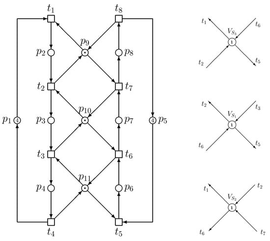
Figure 2.
An PR PN model of AMS (left) and its supervisor (right).
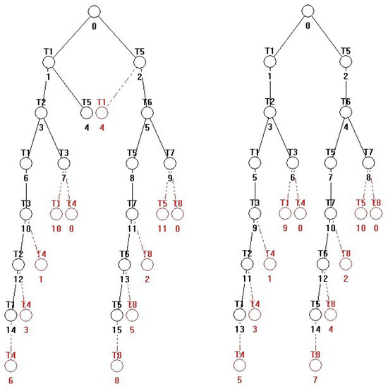
Figure 3.
The RT of the supervised system displayed in Figure 2. On the left, there is an RT corresponding to applying the supervisor consisting of . It can be seen that node 4 represents a deadlock. On the right, there is an RT corresponding to applying the supervisor consisting of . It can be seen that there is no deadlock (node 4 was eliminated), but the other RT parts are identical (as to the structure) with those in the RT on the left. Only the number of nodes is less by one node.
Here, it is necessary to say that the monitor does not follow from the third row of , because monitors were assigned only to elementary siphons.
Firing transition decreases the number of tokens in , and firing decreases the number of tokens in and . Firing decreases the number of tokens in and . Firing decreases the number of tokens in , and firing decreases the number of tokens in . Details are given in Table 2.
Table 2.
Transitions taking away the tokens from siphons.
These facts determine the following procedure and its considerations. Because and are controlled by monitors and , respectively, in order to control , we have to add a token to and (because must not be emptied) and take a token from and (because are controlled). From such a simple consideration, we can construct the monitor —see the upper right side of Figure 2. At an initial marking , , and .
In general, let the marking of , where are markings of , respectively, hold. Evidently, the strongly dependent siphon can never become unmarked. That is to say, this siphon will always be marked provided that and are always guaranteed to be marked.
This procedure is a partial contribution to the deadlock prevention. The functionality of after its adding to and is documented by means of the RT of the supervised system given in Figure 2.
With respect to the approach in [46], this supervisor can be said to be optimal, i.e., maximally permissive.
4.2. Another Approach Using a Complementary Set of SMSs
We can also solve the problem that occurred in Example 1 in Section 4.1 by applying complementary set of the siphon S. The complementary set of an SMS S is the set of operation places which on the one hand are the holders of the resources in S, but on the other hand, they do not belong to S. is the support of a P-invariant. It means that the operation places in will compete for the resources in S with the operation places belonging to S. Consequently, when all tokens marked in S flow into , S will be emptied. In particular, in PR [15], the union of the complementary sets of its elementary siphons is the complementary set of a strongly dependent SMS.
If a siphon , then is called the complementary siphon of S and is the support of a P-invariant. Here, is the minimal siphon containing r. The sum of tokens in is a constant. Thus, forms the support of a minimal P-invariant.
Lemma 5
([85]). Let , while the minimal siphon containing r is (also the support of a minimal P-invariant) with , and .
Corollary 2
([15]). Let be a marked PR, S be an SMS of , and be its complementary set of S. Suppose a control place is added by Proposition 2 [15] such that S is invariant controlled and denote the new net by . Then, is the support of the P-invariant of .
Proposition 2
([15]). Let be an SMS of a net system , where . Add a control place to to make P-vector be a P-invariant of a new net system , where ; and , where is a row vector due to the addition of place . Let where . Then, S is an invariant-controlled SMS and hence always marked at any reachable marking of .
Therefore, we have and, consequently, is a strongly dependent siphon.
Because for , we can write [15] .
Corollary 3
([15]). Let be a strongly dependent SMS with respect to elementary siphons in an PR. We have .
Theorem 5
([15]). Let be a marked PR and be a strongly dependent SMS with respect to elementary siphons . By Definition 8, add n control places such that are controlled with the control depth variables respectively. can never be emptied if , where .
Now, the marking of the supervisor monitors has to be determined. With respect to the initial rubric of Section 3.1.2 concerning the limit controlled S, any unmarked state is reached when or .
Theorem 6
([81,86]). Let be a net system and be strongly dependent SMS with respect to elementary siphons such that where , and if and only if . is extended by n control places so that are limit-controlled. can never be emptied if and only if , .
Note that for strongly dependent siphon is a single resource r, while implies that there is only one token in the initial marking of r.
A siphon S is a set of places where tokens can leak out into another set of places called the complementary set of the siphon.
In [87], a more precise definition is introduced: The complementary set of S, denoted by , is a set of operation places that are not in S but their execution needs the resources contained in SMS. denotes the set of critical transitions of r, where . denotes the set of critical transitions of S.
The term self-max-controlled siphons also exists.
Definition 16
([88]). Given a well-marked PR , a siphon S in N is self-max-controlled if there is a marked trap in it or such that , where ’%’ is modulus operator.
In our case, N in Figure 1 and Figure 5 is and . is max-marked at since
Definition 17
([89]). Let S be a strict minimal siphon in a well-marked PR net . S is said to be -marked (-marked) at if at least one (none) of the following conditions hold:
- ;
- ;
- and (t is enabled at M).
Here, is a binary variable indicating whether the arc is enabled (enabled means: ; disabled means: ).
Definition 18
([89]). Let S be a strict minimal siphon in a well-marked PR net ). S is said to be -controlled if S is -marked at any reachable marking from .
Theorem 7
([89]). Let be a well-marked PR net and be the set of SMSs. It is live if and only if is -controlled.
Applying this theoretical background to the AMS model from Example 1, we can elaborate the following Example 2.
Example 2
Consider the AMS model displayed on the left side of Figure 2. There are .
Hence, we have siphons , where .
In agreement with Definitions 13 and 30, their complementary sets are , respectively.
As it was mentioned above, a minimal siphon S is said to be strict if . Let be a set of SMS of N. Let us have , and . Here, denotes the operation places of operations and denotes resource places.
Definition 19
([82]). Let be a reliable resource place in an PR N. The operation places using resources r are known as the set of holders of r, which is indicated by . is said to be the complementary set of S if .
Definition 20
([17]). Let and be marked Petri nets; , where . We call with a synchronous net resulting from the integration of and and denote it as when the following conditions are satisfied: (1) , and ; (2) ; (3) ; (4) , where ; (5) , where .
Definition 21
([82]). Let be an PR with . The deadlock controller for developed by Ezpeleta et al. (see [37]) is denoted as , where (1) is a set of control places; (2) ; (3) is the set of directed arcs that join the control places with transitions (and vice versa); (4) For all , where is called an initial marking of a control place .
is the support of a P-invariant. It means that the operation places included in [S] will compete for the resources in S with the operation places belonging to S. Then, S will be without tokens (i.e., unmarked) when all tokens in S flow into . This fact can be used in the following control policy.
Concisely said, let S be a strict minimal siphon which does not contain the support of any place semiflow (i.e., a siphon that can be emptied). Then, we have , , . , where indicates the positive support of the place invariant . For the siphon S, is the set of holders, corresponding to resources in S that do not belong to S. For that reason, is said to be the complementary set for S. Due to this fact, a monitor (control place) is added for and the initial marking is .
Hence,
It can be seen on the right side of Figure 4 that no deadlock exists there in the RT; however, the RT does not have as many nodes (PN model states) as that in Example 1. This finding is another part of our contribution (result) to the topic of deadlock prevention.
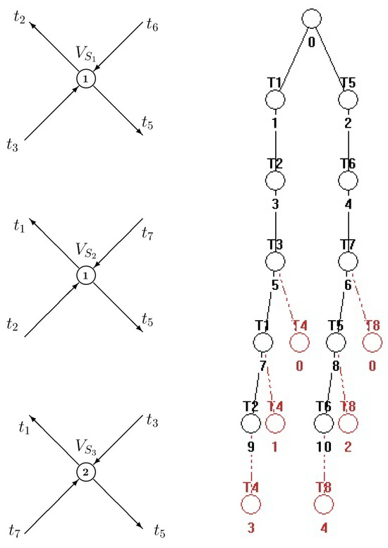
Figure 4.
The supervisor computed by means of the procedure using complementary sets of siphons for the AMS model represented by N in Figure 2 (left) and the corresponding RT of the controlled system (right). It documents that there are no deadlocks in the controlled N; however, the RT does not have as many nodes as that in Example 1.
The next matrix (6) presents the supervisor incidence matrix, while the incidence matrix of the controlled system is shown in (7).
Summary: Upon comparing the results obtained in Example 1 and Example 2, respectively, we can see that the approach to deadlock prevention in Example 1 is more effective and more favorable regarding the size of the state space of the controlled system (i.e., less restricting and makes the behavior of the controlled system more free—its RT yields 14 states vs. 10).
4.3. Simpler AMS with GPN Models
The procedure used for the solution of such problems consists of the application of the following knowledge.
Definition 22
([17]). A siphon S in an ordinary PN is invariant controlled by P-invariant I under the initial marking if and only if and , or equivalently, and . Here, is the positive support of I.
Lemma 6
([39,83]). Let ) be a marked net and S be a siphon of N. S is max-controlled if there exists a P-invariant I such that , , , and .
In a R N, r is a resource place, S is an SMS, and . Let . It can be seen that is true. Let us use to denote . says that siphon S loses just tokens when the number of tokens in p increases by one.
Definition 23
([39,83]). Let the net be a marked net and S be a siphon of N. S is said to be max-controlled if and only if S is max-marked at any reachable marking.
Theorem 8
([25,90]). Let , be a marked net and S be a strongly dependent siphon with , where are elementary siphons of S. S is max-controlled if the following apply:
- 1.
- is a P-invariant of N, , and ;
- 2.
- .
Corollary 4
([90]). Let be an PR net system and S be a strongly dependent siphon with where are the elementary siphons of S. S is max-controlled if the following apply:
- 1.
- is extended by adding n monitors such that are max-controlled, respectively;
- 2.
- , where.
Corollary 5
([90]). Let be an initially well-marked PR net system and S be a weakly dependent siphon with , where are the elementary siphons of S. S is max-controlled if the following apply:
- 1.
- is extended by adding n monitors such that are max-controlled, respectively, due to Proposition 3 (below);
- 2.
- , where
Proposition 3
([90]). Let S be a strict minimal siphon in a marked PR net , where . Construct for S due to Definition 35 (introduced below in Section 4). A monitor is added to by the enforcement that is a P-invariant of the resultant net system , where ; . Let and . Then, S is max-controlled if .
Example 3
Let us use the same basic structure of the AMS model as that in the left side of Figure 1 but with four duple directed arcs—see the left side of Figure 5. This is an PR (extended PR) structure. Siphons are the same because they are structural entities. The supervisor computed using complementary sets of siphons is shown on the right side of Figure 5.
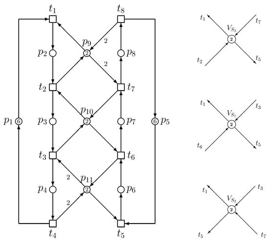
Figure 5.
The GPN N of the kind of PR (left) and its supervisor synthesized by means of the procedure using complementary sets of siphons (right).
The following procedure was used to perform the deadlock prevention. The incidence matrix of this GPN is shown below:
Because of elements greater than 1 in the matrix (8), the marking of resources must be increased, too. Siphons are structural parameters, and they do not depend on the weights of arcs. There are three sets of places in Figure 5: namely, is a set of operation places, is a set of resource places, and is a set of idle places. Siphons create rows of the matrix (9):
Realizing the matrix multiplication , we obtain the matrix (10) expressing the supervisor structure.
Here, we can easily see that the third row of the matrix is the sum of the previous two rows, i.e., . This implies two elementary siphons and and the strongly dependent siphon .
N has five P-invariants: ; ; ; ; or in the matrix form (11):
As we can see, only three of them have something to do with resources (see rows 2, 3 and 4 of the matrix (11)).
Let us rewrite siphons into the multiset form. Thus,
;
;
.
Similarly, there are P-invariants, where the framed elements are concerning the following resources:
;
+ ;
+ ;
+ ;
.
Let r be a resource place, S be an SMS and in an R net. Let us define . We can see that is correct. Use to denote . shows the fact that when the number of tokens in the place p increases by one, the number of tokens in the siphon S decreases by .
Here, ; ; .
.
.
.
Because , and are elementary siphons and is the siphon that is strongly dependent on them. The controllability of can be verified by using Theorem 9 and its Corollaries 4 and 5. and are P-invariants satisfying Theorem 9 (condition (1)).
Seeing that siphons, as structural entities, do not depend on the weights of directed arcs, we have the same siphons as in N displayed in Figure 1 , and . Thus,
Because and ,
i.e., , it can be said that is max-controlled by means of the P-invariant .
The analogical sequence we may apply for the second SMS follows:
Because and ,
i.e., , it can be said that is max-controlled by means of the P-invariant .
Thus, the controllability of the elementary siphons was verified. Now, we will verify the controllability of the strongly dependent siphon . are P-invariants satisfying condition (1) of Theorem 9. Now, condition (2) of Theorem 9 will be verified. . While .
Because 6 > 4, we can say that is max-controlled, too.
The setting of monitors corresponds to Corollary 4 [90].
As we can see from the RT in Figure 6, there are 36 nodes (i.e., 36 states of the state space including the initial state). This result cannot be compared with the results of the previous two examples, because due to the multiplicity of arcs in the PN model, the resources (more precisely the markings of resource places) also had to be increased.
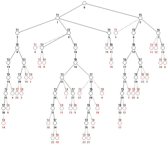
Figure 6.
The RT of the controlled in Figure 5. It documents that there are no deadlocks in the controlled N. The expansiveness of the tree documents the freedom of the controlled system behavior.
4.4. More Complex AMS with OPN Model
Example 4
Consider a more complex system of the structure symbolically expressed in Figure 7. It comprises three robots R1–R3, four machines M1–M4, and three input places I1–I3 as well as three output places O1–O3. In this AMS scheme, robots serve as quasi “conveyors” in order to transfer parts among particular regions of the AMS. The sphere of activity for R1 consists of I1, O1, and M1–M4; the sphere of activity for R2 consists of I2, O3, M1, and M3; and the sphere of activity for R3 consists of I3, O2, M2, and M4. The AMS produces three kinds of products: J1–J3.
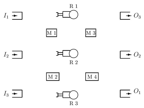
Figure 7.
The scheme of the more complex AMS.
R1 is loading raw materials for J1 to M1, where J1 is fabricated, and unloading finished products J1 to O1. The procedure for the fabrication of J2 is more complicated. Raw materials for J2 and finished products J2 are loaded from I2 and unloaded to O2 by R1 and R3, respectively. Meanwhile, two optional routes for the fabrication of J2 are possible: (i) M1 → R1 → M2, which means that J2 is fabricated by M1 and M2 in such sequence; or (ii) M3 → R1 → M4, which means that J2 is fabricated by M3 and M4 in such sequence. Between M1 and M2 or M3 and M4, the conveying operation from the former (i.e., M1 or M2), to the latter (i.e., M3 or M4) is performed by R1. The final product J2 is obtained at the end of either route.
Raw materials for J3 are loaded from I3 and finished products J3 are unloaded to O3 by R3 and R2, respectively. Meanwhile, J3 is produced by M4 and M3 in sequence, where the conveying operation from the former to the latter is performed by R1.
The PN model in Figure 8 has 18 SMS as follows:
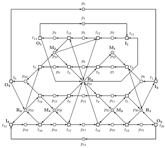
Figure 8.
The PN model of the AMS schematically depicted in Figure 7.
The PN model of this complex is shown in Figure 8.
This SMS set consists of six elementary siphons () and 12 strongly dependent siphons (denoted by *). The relations between dependent siphons and elementary ones follow:
Hence, all siphons denoted by * are strongly dependent siphons.
Expressing elementary siphons in the form of the matrix and consequently, after multiplication , we have
The rank of the matrix is 6. The P-invariants are the rows of the following matrix:
or they have the following form:
The invariants denoted by * do not have anything to do with resources.
Monitors can be marked by means of the inequality , where M means the marking in the PN model of the original plant, while expresses the marking in the extended system (plant + supervisor). Because , it is sufficient to put . Similarly, because , and consequently, it is sufficient to put , , . Analogically, , ; , ; , .
With respect to [15,16], adding a control place for each elementary siphon does not result in the creation of a new SMS. Putting for , we obtain It means that adding a control place for each elementary siphon guarantees that all of the elementary siphons will be in any case marked.
is called the siphon control depth variable. It can also be greater than 1, i.e., . It ensures that the SMS can never be emptied. In the opposite case, a new deadlock originates.
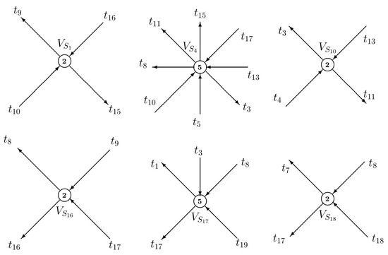
Figure 9.
The supervisor for the PN model in Figure 8. The directed arches show (1) from which PN transitions they come out (i.e., from the set ) and then enter the ; and (2) into which PN transitions they enter after coming out of the (i.e., into the set ), .
As it was shown in [91,92], in general, a deadlock-freeness does not necessarily imply liveness. The main difference between a siphon and a trap is that a siphon with no tokens remains without tokens, while a marked trap remains marked. All transitions associated with an empty siphon are not live. It is also very important that for any marking that does not allow firing any transition, the set of empty places creates a siphon.
5. More Complex GPN Models of AMSs
In this section, the GPN model has the form of an PR (Simple System of Simple Sequential Processes with Shared Resources).
Definition 24
([17]). An R is a generalized connected self-loop-free Petri net where the following apply:
- 1.
- .
- 2.
- is a partition such that (i) is called the set of operation places, where and ; (ii) is called the set of idle places; (iii) is called the set of resource places.
- 3.
- is called the set of transitions, where and .
- 4.
- , the subnet generated by , is a strongly connected state machine such that every circuit of the state machine contains idle place .
- 5.
- , there exists a unique minimal P-semiflow such that , and .
- 6.
- .
Definition 25
([18]). An PR is a connected generalized self-loop free Petri net where the following apply:
- 1.
- is a partition such that the following apply:
- , where for each , and for each , .
- .
- .
- 2.
- , where for each , and for each .
- 3.
- For each , the subnet is a strongly connected state machine such that every cycle contains .
- 4.
- For each , there exists a unique minimal P-invariant such that , and .
- 5.
- .
Definition 26
([18]). Let , be an initially marked PR. Marking is said to be an acceptable initial marking for N if and only if the following apply:
- 1.
- ;
- 2.
- ; and
- 3.
- .
Definition 27
([18]). Let be an acceptably marked PR. Let , and the set of holders of r is the support of a minimal P-invariant without place r, i.e., .
Definition 28
([18]). Let be an acceptably marked PR. Let S be an emptiable siphon, and is called the thieves of S, where , and .
For an arbitrary marking , a transition t is M-process-enabled if and only if such that . Similarly, a transition t is M-resource-enabled if and only if such that [18].
Proposition 4
([18]). Let be an acceptably marked PR. The system is not live if and only if there exists a marking such that the set of M-process-enabled transitions is non-empty and each of them is M-resource-disabled.
Proposition 5
([18]). Let be an acceptably marked PR. The system is not live if and only if there exists a marking and a siphon such that the following apply:
- 1.
- .
- 2.
- .
- 3.
- .
Propositions 4 and 5 ascribe the non-liveness of an PR net to the presence of (i) an insufficiently marked siphon and (ii) a corresponding marking. This is extremely helpful because we can detect and forbid such siphons instead of computing and controlling all SMS; therefore, the number of all SMS exponentially accrues with the size of a PN model. Such an approach may create a skeletal framework of source materials for further publications.
5.1. Properties of Siphons in PR Nets
Definition 29
([17]). For , , the operation places that use r are called the set of holders of r. Let . is called the complementary set of siphon S.
Definition 30
([17]). Let r be a resource place and S be a strict minimal siphon in an R. The holder of resource r is defined as the difference of two multisets and r: . As a multiset, is called the complementary set of siphon S.
Definition 31
([17]). is called the support of complementary set of siphon S.
We can easily see [17] that is true. Let . Then, . Let denote . Then, indicates that siphon S loses tokens if the number of tokens in the place p increases by one. is often named the risk coefficient of the place p.
The set is the set of operation places. Each place is called an idle place. Namely, it represents the state in which the corresponding i-th processes are idle. is a set of resource places.
Proposition 6
([93]). A minimal siphon S in an PR N is an SMS if S is an emptiable minimal siphon (EMS).
Definition 32
([17]). An initial marking is acceptable for an R if and only if (i) ; (ii) ; and (iii) .
Theorem 9
([10,36]). Let S be a strict minimal siphon in an R . Then, satisfies and .
Definition 33
([17]). Let r be a resource place and S be a strict minimal siphon in an R. The holder of resource r is defined as the difference of two multisets and r: . As a multiset, is called the complementary set of siphon S.
Proposition 7
([17]). Let S be a strict minimal siphon in an R net , where . A monitor is added to by the enforcement that is a P-invariant of the resultant net system , where . Let and ). Then, S is max-controlled if and .
is the control depth variable of siphon S. Thus, .
Theorem 10
([17]). Let be an R and S be a strongly dependent siphon with , where are the elementary siphons of S. S is max-controlled if the following apply:
- 1.
- is extended by adding n monitors such that are max-controlled, respectively, due to Proposition 7;
- 2.
- ,where ;
- 3.
- .
Lemma 7
([17]). Let S be a siphon in net and be a marking. S is max-marked under M if , where .
Theorem 11
([17]). Let be an R and S be a weakly dependent siphon with , where are the elementary siphons of S. S is max-controlled if
- 1.
- is extended by adding n monitors such that are max-controlled, respectively, due to Proposition 7;
- 2.
- ,where ;
- 3.
- .
This theorem was proved in [17]. Since is initially well marked, the controllability of a weakly dependent siphon depends only on . That is, its controllability depends on only. Thus, this result is right. is termed well-initially-marked if and only if . This means that a siphon in such a PN has the maximal number of tokens at the initial marking.
Definition 34
([90]). Let be a liveness-enforcing Petri net supervisor of an PR net model , where . , assign a weight α to each place according to a reverse topological numbering on the acyclic state machine induced by if there exists an elementary path from p to ; then, .
Lemma 8
([83,90]). Let ) be a marked net and S be a siphon of N. S is max-controlled if there exists a P-invariant I such that , and .
Proposition 8
([90]). Let S be a strict minimal siphon in a marked PR net , where . Construct for S due to Definition 35 (below). A monitor is added to by the enforcement that is a P-invariant of the resultant net system , where . Let and . Then, S is max-controlled if .
Definition 35
([17,90]). Let S be a strict minimal siphon in an PR plant net model , where . Let such that and . For S, a non-negative P-vector is constructed as follows:
- Step 1 ;
- Step 2 , where ;
- Step 3 , let be such a place that , , . We assume that there are m such places, . Certainly, we have . , let be such a place that . ;
- Step 4 , where , and s.t. .
5.2. Example 5
Consider the AMS with a GPN model as given in Figure 10. Its structure is very similar to that in Figure 8. The difference only is that here, in Figure 10, four directed arcs have the weight 2. They are the arcs and .
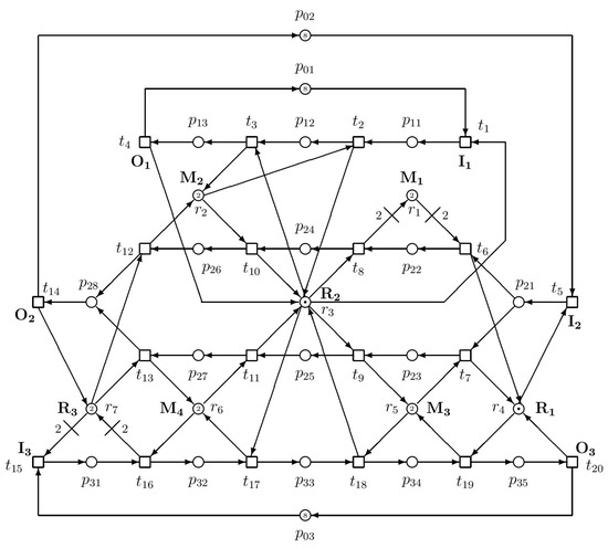
Figure 10.
The PN model of the AMS by PR net.
The functioning of the AMS in Figure 11 is very similar to that in Figure 8. By contrast to Figure 8, a problem only is that two copies of resources are required when M1 elaborates J2 and when R3 conveys J3 from I3 to M4.
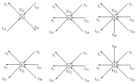
Figure 11.
The supervisor of the AMS PR.
The siphons of this GPN are as follows:
The strict minimal siphons are denoted by *.
Here, we have , . represents the first transition in the ith process. Formally, . Resources correspond to , and , respectively.
Because the structural properties (siphons, traps, invariants) of the PN model displayed in Figure 10 are the same as those in the previous net in Figure 8, we have 10 invariants as follows:
The invariants denoted by * do not have anything to do with resources.
In Figure 10, we have seven resources . Consequently, the corresponding minimal P-semiflows are the following:
In the initial state of the system .
In our example, we have the following holders:
. Hence, the complementary sets of siphons and their supports are as follows:
1. For the siphon ,
As to Proposition 7 [17],
, i.e., e.g., , and
2. For the siphon ,
3. For the siphon ,
e.g., , and
4. For the siphon
5. For the siphon
, e.g., , and
6. For the siphon ,
.
.
.
.
.
, e.g., , and
.
Thus,
.
To avoid confusion, is often used for denoting the set of places contained in as well as .
The controllability of strongly dependent siphons – can be verified by means of Theorem 9 [25,90], as it was demonstrated on the strongly dependent siphon in Example 3 introduced in Section 4.3.
6. Results
In this paper, two principal kinds of deadlock prevention were presented, namely for AMSs modeled by ordinary Petri nets (OPNs) and generalized Petri nets (GPNs), respectively. In both kinds, two approaches were verified—on small AMSs with simpler structures and on larger AMSs with more complicated structures. Both approaches were illustrated by several examples. In all cases, the deadlock prevention was based on Petri net siphons. Namely, the controllability of siphons plays a principal role in all cases. PN siphons are divided into elementary siphons and dependent ones. Empty siphons lead to deadlocks. For each SMS in the PN model of AMSs, a monitor has to be added to prevent it from emptying.
A group of monitors creates a supervisor that prevents all siphons from emptying and thus prevents Petri net-based models of AMSs from deadlocks.
6.1. Deadlock Prevention in Simpler OPN Models of AMSs
The theory of deadlock prevention for the PR model was introduced. The controllability of elementary siphons as well as siphons strongly and weakly dependent on them was presented.
Two illustrative examples were included—Example 1, in order to show deadlock prevention by means of elementary and strongly dependent siphons, as well as Example 2, in order to illustrate the approach of deadlock prevention based on the usage of complementary siphons.
Example 1 in Section 4.1 presents an PR model of an AMS with two processes (production lines) sharing three resources. Its OPN-based model is on the left side of Figure 1. On the right side of Figure 1, the reachability graph (RG) belonging to the net model is depicted. As it can be seen, this RG contains two deadlocks (see nodes 13 and 14). To prevent them, strict minimal siphons (SMS) are computed by means of the tool GPenSIM, which is described in [84]. There are three SMSs: two of them are elementary siphons and the third is a strongly dependent one (on the previous two ones). Figure 2 presents the given model with the supervisor consisting of three monitors –. The first two correspond to two elementary siphons, while is a strongly dependent one.
The problem was that at the given resources (i.e., the markings of – being a unit), the standardly proposed supervisor with monitors was not able to remove both deadlocks—see the left side of Figure 3, where it is clear that the RT node is a deadlock.
Consequently, the third monitor had to be added. However, it was constructed nonstandardly by another approach—see Section 4
Then, after including , all deadlocks are prevented, as it can be seen from the RG on the right side of Figure 3 representing the state space of the model controlled by the completed supervisor. The RG has an abundant number of reachable states (e.g., in comparison with the RG in Figure 4 belonging to Example 2 in Section 4.2). With respect to the approach in [46], this supervisor is optimal, i.e., maximally permissive. This can be understood to be a first result of this paper.
Example 2 in Section 4.2 represents the deadlock prevention of the same model as that in Example 1, but the process of the supervisor synthesis is based on complementary siphons. Three monitors of the supervisor are shown in Figure 4 (left) while the corresponding RG is shown on the right side of Figure 4. Although here, all deadlocks are also prevented, the corresponding RG is not as expansive as that in Example 1. It means that the state space of the model controlled by this supervisor has fewer reachable states than the model in Example 1 in Section 4.1. This finding is another one of our contributions (results) to the topic of deadlock prevention. However, information based on one simple example does not yet provide us with the basis for more serious generalization.
6.2. Deadlock Prevention in Simpler GPN Models of AMS
The theory of deadlock prevention for Extended Systems of Simple Sequential Processes with Resources (PRs) was introduced. The theory for the controllability of elementary siphons as well as siphons strongly and weakly dependent on them utilized a method completely different from those previous used. To synthesize monitors of the supervisor, Theorem 9 was applied. First, the analysis of holders of resources by means of PN P-invariants was performed. Then the complementary set of siphon S had to be computed. The function following from it helps find the corresponding monitor and its interconnections with the original uncontrolled PN model of the AMS as well as set its marking. The procedure consisting of Equations (12)–(27) corresponds to the control synthesis for elementary siphons . For the control of the strongly dependent siphon , condition (2) of the Theorem 9 has to be used.
Example 3 in Section 4.3 was inserted to illustrate deadlock prevention for a GPN by using a method that was completely different from those used in the previous two examples. The structure of the PN model is the same as those in the previous two examples. However, there are four arches with double weights. Already simply because of the existence of arches with such weights, the marking of places representing resources must be higher. This situation is shown on the left side of Figure 5. After the supervisor synthesis by the method described in Section 4.3, we obtained three monitors creating the supervisor displayed on the right side of Figure 5. The RG displayed in Figure 6 shows that there are 36 reachable states, which is a quite a nice number (“freedom”). This result cannot be compared with the results of the previous two examples, because due to the multiplicity of arcs in the PN model, the resources (more precisely markings of resource places) also had to be increased.
6.3. Deadlock Prevention in More Complex OPN Models of AMS
The same theory as that mentioned in Section 4.1, i.e., by elementary siphons as well as siphons strongly and weakly dependent on them, was applied to the deadlock prevention of a more complex OPN model.
Here, the same procedure as that in Example 1 was used, only the computing of the siphons took longer.
Example 4 in Section 4.4 was included to illustrate this application. The scheme of such a plant is displayed in Figure 7, and its OPN model is shown in Figure 8. The net has 18 SMSs. Six of them are elementary siphons, and the other ones are strongly dependent on them. The monitors of the supervisor are depicted in Figure 9. The procedure of synthesizing the supervisor is described in detail in Section 4.4. The RG is too large to be presented here.
6.4. Deadlock Prevention in More Complex GPN Models of AMSs
The theory for the deadlock prevention of Simple Systems of Simple Sequential Processes with Shared Resources (PRs) was introduced and applied in Section 4.
Here, the same procedure as that in Example 3 was used, only the computing of the siphons and setting of the monitors took longer.
To illustrate the deadlock prevention procedure, Example 5 was introduced in Section 5.2. The structure of the model is similar to that in Figure 8, except that the four arches weigh twice as much. This model is displayed in Figure 10. After applying the procedure described in Section 4, we obtained the monitors of the supervisor depicted in Figure 11.
7. Discussion
The results obtained in this paper are applicable for both OPN-based and GPN-based models of AMSs. While the former models are suitable for classical AMSs with simple interactions among devices (the weights of the PN arches are the same as that of the unit), the latter models are appropriate for more modern AMSs with multiple interactions among devices (the weights of PN arches are greater than that of the unit).
Deadlock prevention is an off-line process. The deadlocks have to be prevented before building the real AMS. This is the only way to avoid unnecessary delays and downtimes occurring during the reconstruction of the AMS, which is necessary to eliminate deadlocks that appeared during the already launched operation of the real AMS built without previous deadlock prevention on the mathematical model.
Before diving into the discussion, it is necessary to say that formal methods like fault diagnosis, performance evaluation, etc. are very important for the analysis of technical systems and for their control synthesis. AMSs are no exception in this regard. Mathematical modeling, simulation, supervisory control, etc. are very important parts of deadlock prevention in AMSs. They provide efficient help and knowledge of the construction and real implementation of AMSs. For mathematical descriptions of AMSs and their modeling, creating Petri nets is very effective. The same apparatus is very suitable also for synthesizing the supervisory control, making deadlock prevention possible. From this point of view, an AMS can be perceived as a resource allocation systems (RAS).
There are a multitude of PN-based approaches to deadlock prevention in AMSs. However, there exist two main streams of methods: namely, methods based on (i) reachability trees and P-invariants of PN and (ii) PN siphons and traps. The origin of the former method consists of forbidding states in DESs in such a way that a set of legal PN markings is demarcated by a set of constraints in the form of linear inequalities (so-called General Mutual Exclusion Constraints (GMEC)). In such a case, the PN-based solution exists, and it is maximally permissive (optimal). The latter method, i.e., siphon based control, is a way to effectively prevent the occurrence of deadlocks. Its main aim is to prevent emptying siphons, because empty or insufficiently marked siphons cause deadlocks. In general, especially for AMS models based on GPNs, a policy of siphon-based deadlock prevention usually does not make it possible to find a maximally permissive supervisor.
In this paper, the siphon-based approach was presented for both OPN and GPN based models of AMSs. The obtained results are illustrated in the five corresponding examples. They were described in detail in Section 6.
8. Conclusions
The area of deadlock prevention in complex AMSs is very large. Consequently, there are many development trends in the theory and its applications.
In the future, we would like to pay attention not only to deadlock prevention when it is necessary to know all of the siphons but also other trends where it is not necessary to know absolutely all of the siphons. Also, approaches based on optimization by means of MIP (Mixed Integer Programming) and MILP (Mixed-Integer Linear Programming) are interesting areas for further research for deadlock prevention. In our opinion, robust deadlock control for AMSs seems to be a very promising area of research. The approach based on extended elementary siphons applicable to GPN models of AMSs seems to be very useful, too.
Funding
This research received no external funding.
Data Availability Statement
Data are contained within the article.
Acknowledgments
This work was partially supported by the Slovak Grant Agency for Science VEGA under Grant No. 2/0005/25.
Conflicts of Interest
The author declares no conflicts of interest.
Abbreviations
The following abbreviations are used in this manuscript:
| AMSs | Automated Manufacturing Systems |
| DESs | Discrete-Event Systems |
| FMSs | Flexible Manufacturing Systems |
| PNs | Petri Nets |
| RASs | Resource Allocation Systems |
| OPNs | Ordinary PNs |
| GPNs | Generalized PNs |
| SMSs | Strict Minimal Siphons |
| PRs | Systems of Simple Sequential Processes with Resources |
| PR | Extended PR |
| PR | Generalized PR |
| s | Systems of Simple Sequential Processes with General Resources Requirement |
| PR | Generalized Linear System of Simple Sequential Processes with Resources |
| Rs | Systems of Sequential Systems with Shared Resources |
| PRs | Simple Systems of Simple Sequential Processes with Resources |
References
- Iordache, M.V.; Antsaklis, P.J. Supervisory Control of Concurrent Systems: A Petri Net Structural Approach; Birkhäuser: Boston, MA, USA, 2008. [Google Scholar] [CrossRef]
- Tarjan, R. Depth-First Search and Linear Graph Algorithms. SIAM J. Comput. 1972, 1, 146–160. [Google Scholar] [CrossRef]
- Liu, G.Y.; Barkaoui, K. A survey of siphons in Petri nets. Inf. Sci. 2016, 363, 198–220. [Google Scholar] [CrossRef]
- Yan, M.; Zhu, R.; Li, Z.; Zhou, M. A Siphon-based Deadlock Prevention Policy for a Class of Petri Nets-S3PMR. In Proceedings of the 17th World Congress of the International Federation of Automatic Control, Seoul, Republic of Korea, 6–11 July 2008; pp. 14467–14472. [Google Scholar]
- Chao, Y.C. Computation of Elementary Siphons in Petri Nets For Deadlock Control. Comput. J. 2006, 49, 470–479. [Google Scholar] [CrossRef]
- Hu, H.; Li, Z.W. Liveness Enforcing Supervision in Video Streaming Systems Using Siphons. J. Inf. Sci. Eng. 2009, 25, 1863–1884. [Google Scholar] [CrossRef]
- Chao, D.Y. Max*-controlled siphons for liveness of S3PGR2. IET Control Theory Appl. 2007, 1, 933–936. [Google Scholar] [CrossRef]
- Chao, D.Y.; Chen, J.-T.; Yu, F. A novel liveness condition for S3PGR2. Trans. Inst. Meas. Control 2012, 35, 131–137. [Google Scholar] [CrossRef]
- Hou, Y.F.; Li, Z.W.; Al-Ahmari, A.M.; El-Tamimi, A.-Z.M.; Nasr, E.A. Extended Elementary Siphons and Their Application to Liveness-Enforcement of Generalized Petri Nets. Asian J. Control 2014, 16, 1789–1810. [Google Scholar] [CrossRef]
- Tricas, F.; García-Vallés, F.; Colom, J.M.; Ezpeleta, J. An Iterative Method for Deadlock Prevention in FMS. In Discrete Event Systems; The Springer International Series in Engineering and Computer Science; Boel, R., Stremersch, G., Eds.; Springer: Boston, MA, USA, 2000; Volume 569. [Google Scholar]
- Park, J.; Reveliotis, S.A. Deadlock avoidance in sequential resource allocation systems with multiple resource acquisitions and flexible routings. IEEE Trans. Autom. Control 2001, 46, 1572–1583. [Google Scholar] [CrossRef]
- Tricas, F.; Colom, J.M.; Ezpeleta, J. A solution to the problem of deadlocks in concurrent systems using Petri nets and integer linear programming. In Proceedings of the 11th Europe Simulation Symposium (ESS’99), Erlangen, Germany, 26–28 October 1999; pp. 542–546, ISBN 1-56555-177-X. [Google Scholar]
- Hou, Y.; Zhao, M.; Liu, D.; Hong, L. An Efficient Siphon-Based Deadlock Prevention Policy for a Class of Generalized Petri Nets. Discret. Dyn. Nat. Soc. 2016, 2016, 1–12. [Google Scholar] [CrossRef]
- Liu, D.; Li, Z.W.; Zhou, M.C. A parameterized liveness and ratio-enforcing supervisor for a class of generalized Petri nets. Automatica 2013, 49, 3167–3179. [Google Scholar] [CrossRef]
- Li, Z.W.; Zhou, M.C. Elementary Siphons of Petri Nets and Their Application to Deadlock Prevention in Flexible Manufacturing Systems. IEEE Trans. Syst. Man Cybern.-Part A Syst. Hum. 2004, 34, 38–51. [Google Scholar] [CrossRef]
- Ezpeleta, J.; Colom, J.M.; Martinez, J. A Petri net based deadlock prevention policy for flexible manufacturing systems. IEEE Trans. Robot. Autom. 1995, 11, 173–184. [Google Scholar] [CrossRef]
- Li, Z.W.; Zhou, M.C. Deadlock Resolution in Automated Manufacturing Systems: A Novel Petri Net Approach; Springer: London, UK, 2009. [Google Scholar] [CrossRef]
- Tricas, F.; Garcia-Valles, F.; Colom, J.M.; Ezpeleta, J. A Petri net structure-based deadlock prevention solution for sequential resource allocation systems. In Proceedings of the IEEE International Conference on Robotics and Automation, ICRA 2005, Barcelona, Spain, 18–22 April 2005; pp. 271–277. [Google Scholar] [CrossRef]
- Zhuang, Q.; Dai, W.; Wang, S.G.; Ning, F. Deadlock Prevention Policy for S4PR Nets Based on Siphon. IEEE Access 2018, 6, 50648–50658. [Google Scholar] [CrossRef]
- Hou, Y.; Li, Z.; Zhao, M.; Liu, D. Extended elementary siphon-based deadlock prevention policy for a class of generalised Petri nets. Int. J. Comput. Integr. Manuf. 2014, 27, 85–102. [Google Scholar] [CrossRef]
- Zhong, C.; Li, Z.; Barkaoui, K. Monitor Design for Siphon Control in S4R Nets: From Structure Analysis Points of View. Int. J. Innov. Comput. Inf. Control 2011, 7, 6677–6690. [Google Scholar]
- Cano, E.E.; Rovetto, C.A.; Colom, J.M. An algorithm to compute the minimal siphons in S4PR nets. Discret. Event Dyn. Syst. 2012, 22, 403–428. [Google Scholar] [CrossRef]
- Wang, S.G.; You, D.; Zhou, M.C. A necessary and sufficient condition for a resource subset to generate a strict minimal siphon in S4PR. IEEE Trans. Autom. Control 2017, 62, 4173–4179. [Google Scholar] [CrossRef]
- Ma, T.; Wang, J.; Hu, H. A Strict Minimal Siphon-Based Necessary and Sufficient Condition for Liveness Verification in General Petri Nets. IEEE Access 2025, 13, 53517–53530. [Google Scholar] [CrossRef]
- Li, Z.W.; Zhang, J.; Zhao, M. Liveness-Enforcing Supervisor Design for a Class of Generalized Petri Net Models of Flexible Manufacturing Systems. IET Control Theory Appl. 2007, 1, 955–967. [Google Scholar] [CrossRef]
- Abdul-Hussin, M.H.; Banaszak, Z.A. Siphon-based deadlock prevention for a class of S4PR generalized Petri nets. In Proceedings of the 2017 International Conference on Control, Automation and Information Sciences (ICCAIS), Chiang Mai, Thailand, 31 October–1 November 2017; IEEE Xplore, Electronic: New York, NY, USA, 2017; pp. 239–244. [Google Scholar] [CrossRef]
- Pan, Y.-L.; Tseng, C.-Y.; Chen, J.-C. Enhancement of Computational Efficiency for Deadlock Recovery of Flexible Manufacturing Systems Using Improved Generating and Comparing Aiding Matrix Algorithms. Processes 2023, 11, 3026. [Google Scholar] [CrossRef]
- Kumaran, T.K.; Chang, W.; Cho, H.; Wysk, R.A. A structured approach to deadlock detection, avoidance and resolution in flexible manufacturing systems. Int. J. Prod. Res. 1994, 32, 2361–2379. [Google Scholar] [CrossRef]
- Gligor, V.D.; Shattuck, S.H. On deadlock detection in distributed systems. IEEE Trans. Softw. Eng. 1980, 6, 435–440. [Google Scholar] [CrossRef]
- Wysk, R.A.; Yang, N.-S.; Joshi, S. Resolution of deadlocks in flexible manufacturing systems: Avoidance and recovery approaches. J. Manuf. Syst. 1994, 13, 128–138. [Google Scholar] [CrossRef]
- Gebraeel, N.Z.; Lawley, M.A. Deadlock detection, prevention, and avoidance for automated tool sharing systems. IEEE Trans. Robot. Autom. 2001, 17, 342–356. [Google Scholar] [CrossRef]
- Grobelna, I.; Karatkevich, A. A Deadlock Recovery Policy for Flexible Manufacturing Systems with Minimized Traversing within Reachability Graph. In Proceedings of the 2022 21st International Symposium INFOTEH-JAHORINA (INFOTEH), East Sarajevo, Bosnia and Herzegovina, 16–18 March 2020; pp. 1–6. [Google Scholar] [CrossRef]
- Li, Z.W.; Liu, G.Y.; Hanisch, H.-M.; Zhou, M.C. Deadlock Prevention Based on Structure Reuse of Petri Net Supervisors for Flexible Manufacturing Systems. IEEE Trans. Syst. Man Cybern.-Part A Syst. Hum. 2012, 42, 178–191. [Google Scholar] [CrossRef]
- Čapkovič, F. Sustainability of Automated Manufacturing Systems with Resources by Means of Their Deadlock Prevention. Electronics 2024, 13, 3517. [Google Scholar] [CrossRef]
- Duan, W.; Zhong, C.; Wang, X.; Rehman, A.U.; Umer, U.; Wu, A.N. A Deadlock Prevention Policy for Flexible Manufacturing Systems Modeled With Petri Nets Using Structural Analysis. IEEE Access 2019, 7, 49362–49376. [Google Scholar] [CrossRef]
- Abdallah, I.B.; ElMaraghy, H.A. Deadlock prevention and avoidance in FMS: A Petri net based approach. Int. J. Adv. Manuf. Technol. 1998, 14, 704–715. [Google Scholar] [CrossRef]
- Li, Z.W.; Zhou, M.C.; Wu, N.Q. A Survey and Comparison of Petri Net-Based Deadlock Prevention Policies for Flexible Manufacturing Systems. IEEE Trans. Syst. Man Cybern.-Part C Appl. Rev. 2008, 38, 173–187. [Google Scholar] [CrossRef]
- Huang, Y.S. Design of deadlock prevention supervisors using Petri nets. Int. J. Adv. Manuf. Technol. 2007, 35, 349–362. [Google Scholar] [CrossRef]
- Barkaoui, K.; Abdallah, I.B. A Deadlock Prevention Method for a Class of FMS. In Proceedings of the IEEE International Conference on Systems, Man, and Cybernetics, Vancouver, BC, Canada, 22–25 October 1995; pp. 4119–4124. [Google Scholar] [CrossRef]
- Li, Z.; Shpitalni, M. Smart deadlock prevention policy for flexible manufacturing systems using Petri nets. IET Control Theory Appl. 2009, 3, 362–374. [Google Scholar] [CrossRef]
- More, S.S.; Bhatwadekar, S.D. Analysis of Flexible Manufacturing System using Petri Nets to design a Deadlock Prevention Policy. Int. J. Eng. Res. Technol. (IJERT) 2016, 5, 448–453. [Google Scholar] [CrossRef]
- Zhu, R. A deadlock prevention approach for flexible manufacturing systems with uncontrollable transitions in their Petri net models. Asian J. Control 2011, 14, 217–229. [Google Scholar] [CrossRef]
- Zhong, C.; Li, Z. A deadlock prevention approach for flexible manufacturing systems without complete siphon enumeration of their Petri net models. Eng. Comput. 2009, 25, 269–278. [Google Scholar] [CrossRef]
- Wang, S.G.; Wu, W.H.; Yang, J. Deadlock prevention policy for a class of petri nets based on complementary places and elementary siphons. J. Intell. Manuf. 2015, 26, 321–330. [Google Scholar] [CrossRef]
- Piroddi, L.; Cordone, R.; Fumagalli, I. Selective siphon control for deadlock prevention in Petri nets. IEEE Trans. Syst. Man, Cybern. Part A 2008, 38, 1337–1348. [Google Scholar] [CrossRef]
- Uzam, M. An Optimal Deadlock Prevention Policy for Flexible Manufacturing Systems Using Petri Net Models with Resources and the Theory of Regions. Int. J. Adv. Manuf. Technol. 2002, 19, 192–208. [Google Scholar] [CrossRef]
- Liu, G.; Chao, D.; Uzam, M. Maximally permissive deadlock prevention via an invariant controlled method. Int. J. Prod. Res. 2013, 51, 4431–4442. [Google Scholar] [CrossRef]
- Xing, K.; Zhou, M.C.; Liu, H.; Tian, F. Optimal Petri-Net-Based Polynomial-Complexity Deadlock-Avoidance Policies for Automated Manufacturing Systems. IEEE Trans. Syst. Man Cybern.-Part A Syst. Hum. 2009, 39, 188–199. [Google Scholar] [CrossRef]
- Tricas, F. Deadlock Analysis, Prevention and Avoidance in Sequential Resource Allocation Systems. Ph.D. Dissertation, University of Zaragoza, Zaragoza, Spain, 2003. [Google Scholar]
- Pan, Y.-L. One Computational Innovation Transition-Based Recovery Policy for Flexible Manufacturing Systems Using Petri Nets. Appl. Sci. 2020, 10, 2332. [Google Scholar] [CrossRef]
- Hou, Y.F.; Barkaoui, K. Deadlock analysis and control based on Petri nets: A siphon approach review. Adv. Mech. Eng. 2017, 9, 1–30. [Google Scholar] [CrossRef]
- Lautenbach, K.; Ridder, H. Liveness in bounded Petri nets which are covered by T-invariants. In Applications and Theory of Petri Nets, Lecture Notes in Computer Science; Valette, R., Ed.; Springer: Berlin, Germany, 1994; Volume 815, pp. 358–375. [Google Scholar]
- Lautenbach, K. Linear algebraic calculation of deadlocks and traps. In Concurrency and Nets; Voss, K., Genrich, H.J., Rozenberg, G., Eds.; Advances in Petri Nets; Springer: Berlin/Heidelberg, Germany, 1987. [Google Scholar]
- Unruh, E.; Delfmann, P.; Thimm, M. Quantitative Deadlock Analysis in Petri Nets using Inconsistency Measures. In Proceedings of the 2021 IEEE 3rd Conference on Business Informatics (CBI), Bolzano, Italy, 1–3 September 2021; 10p. [Google Scholar] [CrossRef]
- Thimm, M. On the evaluation of inconsistency measures. In Measuring Inconsistency in Information; Series Studies in Logic; Grant, J., Martinez, M.V., Eds.; College Publications: Melbourne, Australia, 2018; Volume 73, ISBN 9781848902442. [Google Scholar]
- Desel, J.; Kilinc, G. Observable Liveness. In Proceedings of the International Workshop on Petri Nets and Software Engineering, PNSE’14, a Satellite Event of Petri Nets 2014, Tunis, Tunisia, 23–24 June 2014; CEUR Workshop Proceedings, 1160. Moldt, D., Rölke, H., Eds.; Universität Hamburg: Hamburg, Germany, 2014; pp. 143–163. [Google Scholar]
- Zhong, C.; He, W.; Li, Z.; Wu, N.; Qu, T. Deadlock analysis and control using Petri net decomposition techniques. Inf. Sci. 2019, 482, 440–456. [Google Scholar] [CrossRef]
- Grobelna, I.; Karatkevich, A. Deadlock detection in Petri nets: One trace for one deadlock? In Proceedings of the 7th International Conference on Human System Interactions (HSI), Lisbon, Portugal, 16–18 June 2014; 5p. [Google Scholar] [CrossRef]
- Kim, J.; Lee, J. Efficient Deadlock Detection in FMS Based on the Transitive Matrix of Resource Share Places. In Proceedings of the 23rd International Technical Conference on Circuits/Systems, Computers and Communications (ITC-CSCC 2008), Shimonoseki City, Japan, 6–9 July 2008; pp. 277–280. [Google Scholar]
- Kim, S.; Lee, S.; Lee, J. Deadlock Analysis of Petri Nets Based on the Resource Share Places Relationship. Stud. Inform. Control 2007, 16, 33–44. [Google Scholar] [CrossRef]
- Bashir, M.; Zhou, J.; Muhammad, B.B. Optimal Supervisory Control for Flexible Manufacturing Systems Model with Petri Nets: A Place-Transition Control. IEEE Access 2021, 9, 58566–58578. [Google Scholar] [CrossRef]
- Yamalidou, K.; Moody, J.; Lemmon, M.; Antsaklis, P. Feedback control of Petri nets based on place invariants. Automatica 1996, 32, 15–18. [Google Scholar] [CrossRef]
- You, D.; Guang, W.S.; Zhou, M.C. Computation of strict minimal siphons in a class of Petri nets based on problem decomposition. Inf. Sci. 2017, 409–410, 87–100. [Google Scholar] [CrossRef]
- Chu, F.; Xie, X.-L. Deadlock Analysis of Petri Nets Using Siphons and Mathematical Programming. IEEE Trans. Robot. Autom. 1997, 13, 793–804. [Google Scholar] [CrossRef]
- Chao, Y.D. Revised dependent siphon. Int. J. Adv. Manuf. Technol. 2009, 43, 182–188. [Google Scholar] [CrossRef]
- Li, Z.W.; Uzam, M.; Zhou, M.C. Comments on “Deadlock Prevention Policy based on Petri Nets and Siphons”. Int. J. Prod. Res. 2004, 42, 5253–5254. [Google Scholar] [CrossRef]
- Hu, H.; Liu, Y.; Yuan, L. Supervisor Simplification in FMSs: Comparative Studies and New Results Using Petri Nets. IEEE Trans. Control Syst. Technol. 2016, 24, 81–95. [Google Scholar] [CrossRef]
- Wu, Y.; Xing, K.; Luo, J.; Feng, Y. Robust deadlock control for automated manufacturing systems with an unreliable resource. Inf. Sci. 2016, 346, 17–28. [Google Scholar] [CrossRef]
- Bashir, M.; Li, Z.; Uzam, M.; Wu, N.; Al-Ahmari, A. On structural reduction of liveness-enforcing Petri net supervisors for flexible manufacturing systems: An algebraic approach. IMA J. Math. Control Inf. 2018, 35, 1217–1249. [Google Scholar] [CrossRef]
- Cong, X.; Wang, A.; Chen, Y.; Wu, N.; Qu, T.; Khalgui, M.; Li, Z. Most permissive liveness-enforcing Petri net supervisors for discrete event systems via linear monitors. ISA Trans. 2019, 92, 145–154. [Google Scholar] [CrossRef] [PubMed]
- Li, Z.W.; Hu, H.S.; Wang, A.R. Design of Liveness-Enforcing Supervisors for Flexible Manufacturing Systems Using Petri Nets. IEEE Trans. Syst. Man-Cybern.-Part C Appl. Rev. 2007, 37, 517–526. [Google Scholar] [CrossRef]
- Wang, S.G.; Wang, C.Y.; Zhou, M.C.; Li, Z.W. A Method to Compute Strict Minimal Siphons in a Class of Petri Nets Based on Loop Resource Subsets. IEEE Trans. Syst. Mans Cybern.-Part A Syst. Hum. 2012, 42, 226–237. [Google Scholar] [CrossRef]
- Chen, Y. Optimal Supervisory Control of Flexible Manufacturing Systems. Ph.D. Thesis, Computer Science, Conservatoire National des Arts et Metiers–CNAM, École Doctorale Informatique, Télécommunications et Electronique de Paris, Paris, France, 2015. Available online: https://theses.hal.science/tel-01288919 (accessed on 29 July 2025).
- Liu, G. Supervisor Synthesis for Automated Manufacturing Systems Based on Structure Theory of Petri Net. Ph.D. Thesis, Automatic Control Engineering, Conservatoire National Des Arts et Metiers—CNAM, École Doctorale Informatique, Télécommunications et Electronique de Paris, Paris, France, 2014. (In English). [Google Scholar]
- Chao, D.Y. Improved Controllability Test for Dependent Siphons in S3PR Based on Elementary Siphons. Asian J. Control 2010, 12, 377–391. [Google Scholar] [CrossRef]
- Uzam, M.; Li, Z.W.; Abukubar, U.S. A General Approach for the Computation of a Liveness Enforcing Supervisor for the Petri Net Model of an FMS. In Proceedings of the 1st International Workshop on Petri Nets for Adaptive Discrete-Event Control Systems—ADECS 2014 (Co-Located with 35th International Conference on Application and Theory of Petri Nets and Concurrency (Petri Nets 2014), Tunis, Tunisia, 24 June 2014; Uzam, M., Li, Z.W., Abubakar, U.S., Eds.; University of Carthage: Carthage, Tunisia, 2014; pp. 1–15. [Google Scholar]
- Nasr, E.A.; Tamimi, A.M.; Al-Ahmari, S.; Kaid, H. Comparison and Evaluation of Deadlock Prevention Methods for Different Size Automated Manufacturing Systems. Math. Probl. Eng. 2015, 2015, 537893. [Google Scholar] [CrossRef]
- Wang, A.R.; Li, Z.W.; Jia, J.Y. A Petri nets based deadlock avoidance policy for flexible manufacturing systems. In Proceedings of the 30th Annual Conference of IEEE Industrial Electronics Society, IECON 2004, Chicago, IL, USA, 2–6 November 2004; Volume 2, pp. 1896–1901. [Google Scholar] [CrossRef]
- Li, Z.W.; Zhou, M.C. Clarifications on the Definitions of Elementary Siphons in Petri Nets. IEEE Trans. Syst. Man Cybern.-Part A Syst. Hum. 2006, 36, 1227–1229. [Google Scholar] [CrossRef]
- Liu, X.; Wang, A.; Li, Z. A Fast Algorithm to Find a Set of Elementary Siphons for a Class of Petri Nets. In Proceedings of the 2006 IEEE International Conference on Automation Science and Engineering, Shanghai, China, 7–10 October 2006; pp. 399–404. [Google Scholar] [CrossRef]
- Chao, D.Y.; Wu, K.-C.; Chen, J.-T.; Lee, M.Y.J. Controllability of Strongly and Weakly Dependent Siphons under Disturbanceless Control. Intell. Control Autom. 2011, 2, 310–319. [Google Scholar] [CrossRef]
- Kaid, H.; Al-Ahmari, A.; Li, Z.; Davidrajuh, R. Single Controller-Based Colored Petri Nets for Deadlock Control in Automated Manufacturing Systems. Processes 2020, 8, 21. [Google Scholar] [CrossRef]
- Barkaoui, K.; Pradat-Peyre, J.F. On Liveness and Controlled Siphons in Petri Nets. In Proceedings of the 17th International Conference on Applications and Theory of Petri Nets, Osaka, Japan, 24–28 June 1996; Lecture Notes in Computer Science. Springer: Berlin/Heidelberg, Germany, 1996; Volume 1091, pp. 57–72. [Google Scholar] [CrossRef]
- Davidrajuh, R. Modeling Discrete-Event Systems with GPenSIM: An Introduction; Springer Briefs in Applied Sciences and Technology; Springer: Cham, Switzerland, 2018; 155p, ISBN 978-3-319-73102-5. Available online: https://link.springer.com/content/pdf/10.1007/978-3-319-73102-5 (accessed on 13 March 2025).
- Chao, D.Y.; Pan, Y.-L.; Liao, W.-H. Structure Based Derived Uniform Formula for Siphon, Its Complementary Set and T-characteristic Vectors. In Proceedings of the 7th IFAC Conference on Manufacturing Modelling, Management, and Control, Saint Petersburg, Russia, 19–21 June 2013; pp. 301–306. [Google Scholar] [CrossRef]
- Shih, Y.-Y.; Chao, D.Y. Sequence of Control in S3PMR. Comput. J. 2009, 53, 1691–1703. [Google Scholar] [CrossRef]
- Liu, G.Y.; Li, Z.W.; Al-Ahmari, A. Liveness Analysis of Petri Nets Using Siphons and Mathematical Programming. In Proceedings of the 12th IFAC/IEEE Workshop on Discrete Event Systems, Cachan, France, 14–16 May 2014; pp. 383–387. [Google Scholar] [CrossRef]
- Liu, G.Y.; Zhang, C.L.; Chang, L.; Al-Ahmari, A.; Wu, N.Q. Robust deadlock control for automated manufacturing systems based on elementary siphon theory. Inf. Sci. 2020, 510, 165–182. [Google Scholar] [CrossRef]
- Liu, G.; Barkaoui, K. Necessary and sufficient liveness condition of GS3PR Petri nets. Int. J. Syst. Sci. 2015, 46, 1147–1160. [Google Scholar] [CrossRef]
- Li, Z.W.; Uzam, M.; Zhou, M.C. Deadlock control of concurrent manufacturing processes sharing finite resources. Int. J. Adv. Manuf. Technol. 2008, 38, 787–800. [Google Scholar] [CrossRef]
- Barkaoui, L.; Couvreur, J.-M.; Klai, K. On the Equivalence Between Liveness and Deadlock-Freeness in Petri Nets. In Proceedings of the 26th International Conference, Applications and Theory of Petri Nets, ICATPN 2005, Miami, FL, USA, 20–25 June 2005; Lecture Notes in Computer Science. Ciardo, G., Darondeau, P., Eds.; Springer: Berlin/Heidelberg, Germany, 2005; Volume 3536, pp. 90–107. [Google Scholar] [CrossRef]
- Gu, C.; Ma, Z.; Li, Z. Liveness and deadlock-freeness verification and enforcement in bounded Petri nets using basis reachability graphs. Automatica 2024, 164, 111625. [Google Scholar] [CrossRef]
- Wang, S.; Duo, W.; Guo, X.; Jiang, X.; You, D.; Barkaoui, K.; Zhou, M.C. Computation of an Emptiable Minimal Siphon in a Subclass of Petri Nets Using Mixed-Integer Programming. IEEE/CAA J. Autom. Sin. 2021, 8, 219–226. [Google Scholar] [CrossRef]


Disclaimer/Publisher’s Note: The statements, opinions and data contained in all publications are solely those of the individual author(s) and contributor(s) and not of MDPI and/or the editor(s). MDPI and/or the editor(s) disclaim responsibility for any injury to people or property resulting from any ideas, methods, instructions or products referred to in the content. |
© 2025 by the author. Licensee MDPI, Basel, Switzerland. This article is an open access article distributed under the terms and conditions of the Creative Commons Attribution (CC BY) license (https://creativecommons.org/licenses/by/4.0/).