Automatic Labeling of Real-World PMU Data: A Weakly Supervised Learning Approach

Abstract

This paper presents a weakly supervised learning framework for real-world event identification in transmission networks using phasor measurement unit (PMU) data. The growing integration of renewable energy sources has introduced greater variability in grid conditions, intensifying the need for accurate event detection. Although high-resolution PMU measurements enable event identification to be formulated as a classification problem, traditional supervised learning approaches are hindered by the scarcity of labeled data, and acquiring large-scale, high-quality labeled PMU datasets remains prohibitively expensive. To overcome this challenge, we propose an automated PMU data-labeling method that combines domain knowledge with machine learning techniques through the use of labeling functions. A novel t-cherry junction tree-based estimation algorithm is introduced to enhance label accuracy, and a greedy strategy is employed to reduce computational complexity. These components are integrated into a weakly supervised framework capable of training robust event classifiers using limited labeled data and abundant unlabeled data. Extensive experiments on real-world PMU datasets demonstrate that our approach achieves competitive accuracy with significantly fewer labeled samples compared to conventional data-driven methods, highlighting its adaptability and resilience under real-world conditions.

1. Introduction

1.1. Motivation

The catastrophic blackout that engulfed Spain on 28 April 2025 caused widespread disruptions with estimated economic losses surpassing EUR 2.25 billion [1]. This event starkly underscores the imperative for advanced real-time monitoring and rapid event detection capabilities in modern power systems. A similar urgency was evident during the 2021 Texas winter blackout, where the lack of an efficient fault classification system delayed critical protective measures—such as activating freeze protection for natural gas wellheads and anti-icing mechanisms for wind turbines. The ensuing cascading failures incapacitated 50% of natural gas generation and 40% of wind power capacity, severely aggravating the electricity crisis.

In recent years, the proliferation of phasor measurement units (PMUs) has transformed power grid observability by facilitating high-resolution data acquisition (e.g., 30–60 samples per second in the U.S.). This technological advancement has unlocked unprecedented potential for real-time situational awareness, rapid event detection, and anomaly identification. Notably, operational successes like the PJM Interconnection in the United States exemplify the tangible benefits of smart grid technologies, enabling real-time monitoring and automated dispatching across an extensive network of 65,000 miles of transmission lines while markedly enhancing system reliability [2].

A fundamental challenge persists in leveraging PMU data for machine learning: the scarcity of accurately labeled datasets required to train reliable models. While supervised approaches, such as Convolutional Neural Networks (CNNs) [3], depend on high-quality labeled data, real-world PMU measurements—such as those collected from the Texas Interconnection under the DOE’s Synchrophasor Data program [4]—are frequently unlabeled, noisy, and corrupted by artifacts (e.g., timestamp errors, data dropouts, and bad measurements). Manual annotation by domain experts remains prohibitively expensive, leaving researchers to rely on sparse or incomplete event logs for model training.

Furthermore, different event types exhibit distinct signal patterns, necessitating a combination of temporal, spectral, and spatial features for accurate detection. For example, transient faults, line outages, and generator tripping events each manifest unique signatures in PMU data. Weak supervision frameworks, such as Snorkel [5], attempt to alleviate labeling constraints by aggregating heuristic rules or noisy labels. However, Snorkel’s ensemble-based approach primarily models label dependencies while failing to capture the intricate temporal and spatial dynamics inherent in PMU signals. Its reliance on static, manually defined labeling functions—which demand substantial domain expertise—restricts adaptability across diverse event signatures, particularly when ground-truth data are limited or noisy. Additionally, Snorkel’s performance is highly sensitive to the design and coverage of its labeling functions; suboptimal heuristics can introduce bias or amplify noise. These challenges are exacerbated by the severe imbalance between the small volume of labeled data and the vast quantities of unlabeled PMU measurements in real-world grid operations.

Our work seeks to address these gaps by exploring methods to automate PMU data labeling with higher accuracy and adaptability, leveraging both domain knowledge and advanced machine learning techniques to bridge the divide between sparse labels and abundant unlabeled data.

1.2. Related Work

Current approaches to addressing the PMU data-labeling challenge can be categorized into four main paradigms: synthetic data generation, unsupervised learning, semi-supervised learning, and weakly supervised learning.

Synthetic Data Approaches. Recent studies have explored synthetic data generation [6] through simulation methods [7,8] and Generative Adversarial Networks (GANs) [9], along with transfer learning [10], ensemble learning [11], and kernelized tensor decomposition models [12]. While these methods can expand training datasets, they often fail to capture the complex dynamics and nuanced characteristics of real-world grid operations. This limitation frequently results in poor generalization performance when the synthetic-trained classifiers are applied to actual PMU data.

Unsupervised Learning Techniques. To leverage abundant unlabeled PMU data, researchers have developed various unsupervised approaches including clustering methods [13], low-rank approximation [14], PCA-based techniques [15,16], and convolutive dictionary learning [17]. However, these methods face fundamental challenges in automatically determining optimal cluster numbers corresponding to different event types. Without labeled guidance, unsupervised techniques may misclassify normal operations as events or fail to distinguish between similar event signatures, potentially introducing significant errors in the resulting classifiers.

Semi-Supervised Learning (SSL) Methods. SSL approaches including self-training [18,19,20], hidden structure models [21], adversarial SSL [22], and CNN-based SSL [23,24] attempt to bridge the gap by combining limited labeled data with abundant unlabeled data. While theoretically promising, these methods exhibit three critical limitations: (i) heavy dependence on predefined, inflexible models; (ii) performance degradation with severely limited labeled data; (iii) inability to effectively incorporate domain knowledge about event characteristics.

Weakly Supervised Learning. Compared to traditional approaches, weakly supervised learning offers distinct advantages in limited labeled data scenarios, including the following:

• Enabling the utilization of noisy, imperfect labels.
• Incorporating fuzzy logic for noise-tolerant confidence quantification.

This approach proves particularly valuable when facing the following:

• Prohibitive annotation costs.
• Non-stationary data distributions.
• Need for domain knowledge integration.

Recent developments like Snorkel [5] implement data programming principles [25], allowing domain experts to encode knowledge through labeling functions. However, Snorkel’s current implementation suffers from several limitations: (i) oversimplification of PMU signal temporal–spatial dynamics; (ii) heavy dependence on expert-designed static labeling functions; and (iii) sensitivity to labeling function quality and coverage.

These shortcomings are exacerbated by the fundamental imbalance between limited labeled data and massive volumes of unlabeled PMU measurements in real-world grid systems.

1.3. Main Contributions

Building upon our previous work [26], which employed Snorkel to estimate the joint distribution for labeling phasor measurement unit (PMU) data, this paper investigates a novel approach based on the t-cherry junction tree for the automatic labeling of real-world PMU data. In contrast to Snorkel, the t-cherry junction tree offers theoretical guarantees for approximation accuracy and supports efficient and exact inference. The key contributions of this work are summarized as follows:

• We propose a novel weakly supervised learning framework that leverages the t-cherry junction tree to approximate the underlying dependencies among labeling functions. By incorporating domain knowledge through structured labeling functions, the framework is capable of classifying both frequent and rare/unseen events. This enables the generation of accurate label estimates from limited labeled data, facilitating the scalable and automatic annotation of PMU datasets for utility applications.
• To address the computational challenges associated with junction tree construction, we design an efficient greedy search algorithm that significantly reduces the search space for optimal t-cherry structures. This ensures high-quality inference while keeping computational overhead manageable.
• We implement the proposed framework to augment scarce labeled training data and evaluate it using two years of real-world PMU measurements from the Western Interconnection of the U.S. transmission grid. Experimental results demonstrate that when labeled data account for less than 15% of the total training set, our approach achieves substantially higher label estimation accuracy than existing state-of-the-art weak supervision models. These results highlight the brilliant performance of unseen events and the potential of the proposed method for practical deployment in large-scale PMU data-labeling tasks.

The rest of the paper is organized as follows: Section 2 provides the details of the proposed weakly supervised learning framework. Section 3 evaluates the performance of event classifiers trained under the proposed framework. Section 4 concludes the paper.

2. Weakly Supervised Learning Based Automatic PMU Data Labeling

2.1. Weakly Supervised Learning Framework

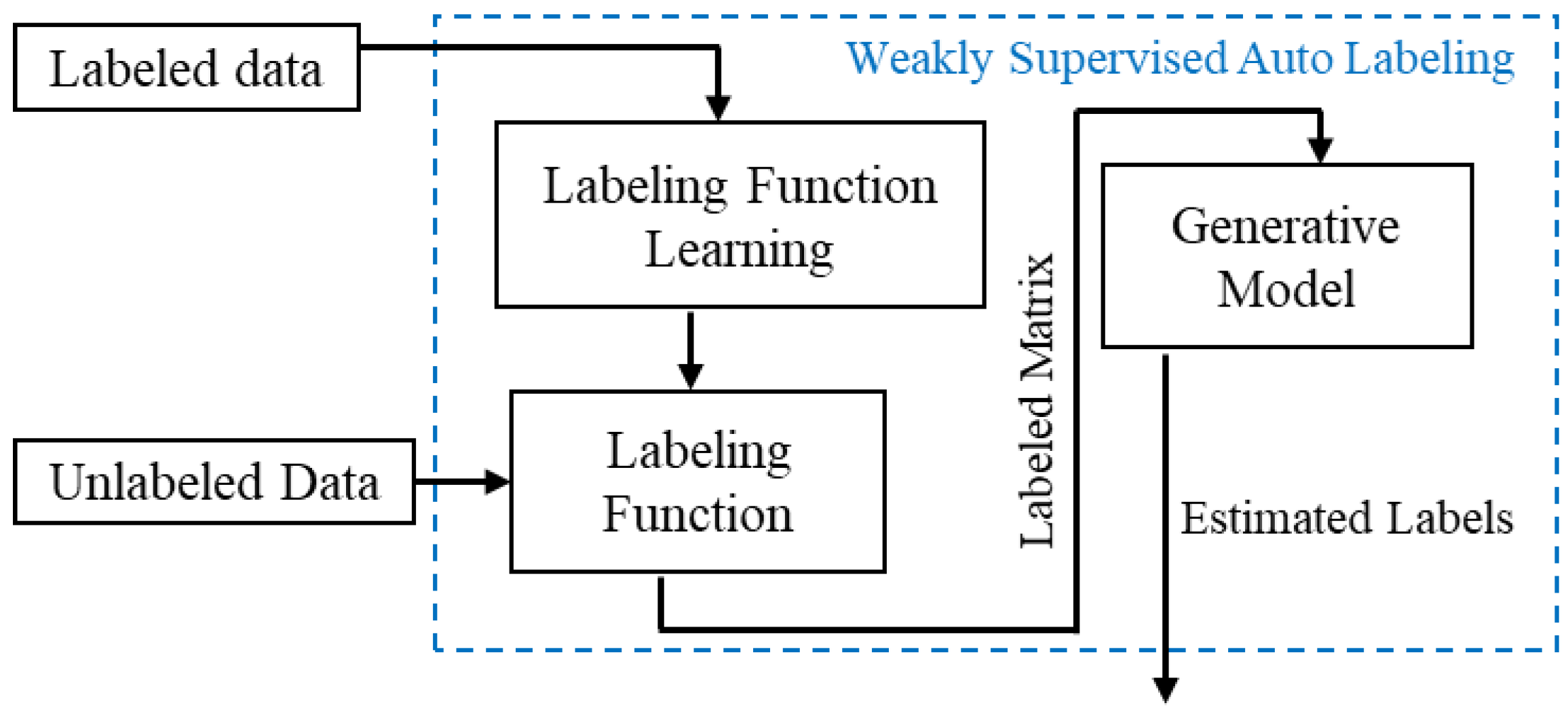
A weakly supervised learning framework (see Figure 1) is proposed to estimate the labels of large amounts of unlabeled PMU data for training event classifiers. As the raw PMU data are often of low quality (e.g., bad data, dropouts, and timestamp errors), the data quality issues are initially fixed before using the proposed framework to estimate the labels, where the data preprocessing proposed in our recent work [4] is carried out and event features are constructed from the PMU data. Then, the labels of unlabeled PMU data are estimated in two main steps: labeling function learning and generative model-based label estimation.

• Labeling function learning. Labeling functions (LFs) can be treated as event classifiers. Given the input PMU data, an LF outputs a label (i.e., event type), e.g., line outage, transformer outage, or frequency event. In the proposed framework, multiple LFs are learnt to characterize the features of different event types. Due to the limited labeled PMU data, the learnt LFs can be noisy and biased. Therefore, directly using the estimates from the LFs cannot generate good event classifiers.
• Generative model. To enhance the accuracy of the estimated labels from the LFs, a generative model is developed. As LFs are learnt using the same dataset, the estimated labels from the LFs are correlated. The goal of the generative model is to characterize the dependency structure of the LFs, based on which the estimated labels are better combined from the LFs to generate better estimates without knowing the ground truth.

Using the estimated labels from the generative model together with the limited labeled data, event classifiers are trained, where different off-the-shelf machine learning models (e.g., random forest) can be used. In the following, the details of each main step in the proposed framework are discussed.

2.2. Labeling Function Learning

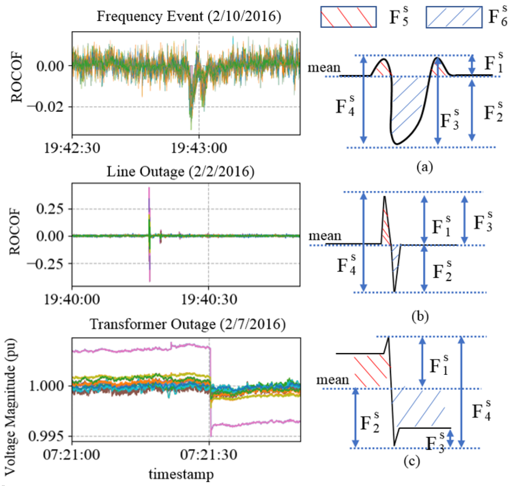
In our earlier study [4], we identified unique patterns in PMU (phasor measurement unit) measurement signals that correspond to various event types, as illustrated in Figure 2. For instance, frequency events display a characteristic wide and deep V-shape, while line outages are marked by a sharp, narrow spike. In contrast, transformer outages take on the form of a step function. By capitalizing on these distinctive signal characteristics, we derived multiple event-specific features $F_i^s$ for each measurement signal s. These features include key parameters such as the amplitude of the signal, the area above or below its average value, and the rates of increase (ramp-up) and decrease (ramp-down) [4].

It is important to note that the classification of event types is determined by considering these collective features rather than isolating individual signal types for analysis. This approach of designing tailored features provides a more comprehensive and nuanced representation of the diverse event patterns. As a result, the event classifiers trained using these features demonstrate significantly greater robustness and accuracy when compared to classifiers that rely solely on raw PMU measurement data [4]. Building on this foundation, we further developed several labeling functions (LFs) from these distinct features, enabling a more refined categorization of different event types.

Let $\mathcal{B}=\{({\mathbf{x}}_1,y_1),\dots ,({\mathbf{x}}_l,y_l),{\mathbf{x}}_{l+1},{\mathbf{x}}_{l+2},\dots ,{\mathbf{x}}_m\}$ represent the training dataset, which consists of m total training samples. Each ${\mathbf{x}}_i$ corresponds to a set of constructed features $F_i^s$ derived from previous work [4], where $F_i^s$ encapsulates key characteristics of the training sample (event). In this dataset $\mathcal{B}$, only l of the samples are labeled, while $m-l$ samples are unlabeled, with $y_i$ denoting the corresponding event label for each labeled sample, where $i=1,2,\dots ,l$. A notable highlight is that the number of labeled data points is significantly smaller than the total size of the dataset, that is, $l\ll m$.

Despite the scarcity of labeled samples, multiple labeling functions (LFs) are trained using various machine learning models, such as Random Forest (RF), Logistic Regression (LR), K-Nearest Neighbor (KNN), and Gradient Boosting Decision Tree (GBDT). These models are trained using the features constructed from different measurement signals, which include voltage magnitude, current magnitude, and the rate of change of frequency (ROCOF). Additionally, combinations of these signals are employed to provide a richer feature set. The different features are used to train the machine learning models for building multiple LFs.

Table 1. LFs built by different features and classifiers, LFs combination 1.

	Classifier	RF	LR	KNN	GBDT
Feature
Voltage magnitude		${\lambda }_1$	${\lambda }_2$	${\lambda }_3$	${\lambda }_4$
ROCOF		${\lambda }_5$	${\lambda }_6$	${\lambda }_7$	${\lambda }_8$

presents the possible LFs that can be constructed by employing various combinations of features and models, where each LF is represented as ${\lambda }_j$. We employ these models as label functions to allow a fair comparison with SSL (semi-supervised learning) and avoid poorly designed heuristics. Since SSL is inherently limited to well-developed models, weakly supervised learning offers greater flexibility by incorporating domain knowledge into label functions.

Suppose k LFs (i.e., $\{{\lambda }_j,j=1,2,\dots ,k\}$) are learnt using the l labeled samples. The output of each LF, i.e., ${\lambda }_j\left({\mathbf{x}}_i\right)$ for $i=l+1,\dots ,m$, is the estimate of the event label of the unlabeled data. Let $\Lambda$ be the label matrix generated by the k LFs for the unlabeled data, where ${\Lambda }_{i,j}={\lambda }_j\left({\mathbf{x}}_i\right)$ for $i\in [l+1,m]$ and $j\in [1,k]$. For a given unlabeled data ${\mathbf{x}}_i$, the outputs from k LFs (i.e., ${\Lambda }_{i,j}$ for $j\in [1,k]$) can be treated as noisy votes. From these noisy votes, it aims to estimate the “true” label without knowing the ground truth.

As LFs are learnt using the same dataset with scarce labels, the estimated labels (i.e., ${\Lambda }_{i,j}$) are often correlated, and the estimates can be noisy and biased. Simply using the majority vote to combine ${\Lambda }_{i,j}$ for $j\in [1,k]$ cannot obtain a good estimate, as the majority vote assumes that the LFs are independent. To enhance the accuracy of the estimated labels, it is of paramount importance to characterize the correlations among the LFs, based on which ${\Lambda }_{i,j}$ for $j\in [1,k]$ can be better combined. Therefore, domain knowledge can be seamlessly integrated into the labeling functions, while the method of constructing labeling functions is not unique.

2.3. Generative Model

To better estimate the true labels Y using $\Lambda$, a generative model is leveraged, where the output of each LF, i.e., ${\Lambda }_{i,j}$, is modeled as a random variable. Using the observation matrix $\overline{\Lambda }$ (i.e., the outputs of $\Lambda$ using the unlabeled data), the joint distribution $\mathrm{Prob}(\Lambda ,Y)$ of this generative model is estimated. $\mathrm{Prob}(\Lambda ,Y)$ will be used to estimate the accuracy of each LF based on how well the $\Lambda$ values are combined to estimate Y. Specifically, the joint distribution can be specified as shown below:

$$\begin{array}{c}\hfill \mathrm{Prob}(\Lambda ,Y)\propto \exp \left(\sum _{i=l+1}^m\sum _{d\in \mathcal{D}}{\theta }_d{\varphi }_d({\Lambda }_i,y_i)\right),\end{array}$$

(1)

where ${\Lambda }_i=({\Lambda }_{i,1},\dots {\Lambda }_{i,k})$ denotes the vector of the estimated labels from k LFs for the training sample i. $\mathcal{D}$ is a set of tuples that describe the dependencies between LFs, denoted by ${\varphi }_d({\Lambda }_i,y_i)$, and ${\theta }_d$ denotes how correlated the LFs are. For example, if d refers to the dependency between two LFs $j_1$ and $j_2$, then ${\varphi }_d({\Lambda }_i,y_i)={\varphi }_{j_1,j_2}({\Lambda }_i,y_i)=\mathbb{1}\{{\Lambda }_{i,j_1},{\Lambda }_{i,j_2}\}$, where the indication function $\mathbb{1}\{{\Lambda }_{i,j_1},{\Lambda }_{i,j_2}\}$ represents whether LFs $j_1$ and $j_2$ depend on each other. As Y is unknown for the unlabeled data, therefore, the distribution $\mathrm{Prob}(\Lambda )$ will be estimated.

To estimate $\mathrm{Prob}(\Lambda )$, we propose using a t-cherry junction tree in this paper. Compared with Snorkel, which was used in our previous work [26], the t-cherry junction tree can offer better approximation (in terms of minimizing Kullback–Leibler divergence), because it has been proved in [27] that the best possible approximation is contained in the junction tree sets. In the following, we discuss how to generate the t-cherry junction tree to estimate $\mathrm{Prob}(\Lambda )$.

2.4. T-Cherry Junction Tree Based Distribution Estimation

2.4.1. Joint Distribution Estimation

A junction tree can be defined as a tree structure over different LFs with each node representing an LF. The outcome of each LF can be viewed as a random variable. To estimate the joint distribution $\mathrm{Prob}(\Lambda )$ using a t-cherry junction tree, we first introduce the concepts of cluster and separator [28]:

• Cluster: Each node of the junction tree is a subset of the LFs, i.e., ${\Lambda }_j\left({\mathbf{x}}_i\right)$, also known as a cluster denoted as ${\Lambda }_C$ with the distribution $\mathrm{Prob}\left({\Lambda }_C\right)$.
• Separator: A separator is an edge that connects two clusters, which can be denoted as ${\Lambda }_s={\Lambda }_{C_1}\cap {\Lambda }_{C_2}$. The separator is also a subset of the LFs, and its distribution can be denoted as $\mathrm{Prob}\left({\Lambda }_s\right)$.

Using the clusters and the separators, the joint distribution can be estimated as shown below:

$$\begin{array}{c}\hfill \mathrm{Prob}\left({\Lambda }_1,\dots ,{\Lambda }_k\right)={\displaystyle \frac{{\displaystyle \prod _{c\in \mathcal{C}}}\mathrm{Prob}\left({\Lambda }_c\right)}{{\displaystyle \prod _{s\in \mathcal{S}}}{\left(\mathrm{Prob}\left({\Lambda }_s\right)\right)}^{v_s-1}}},\end{array}$$

(2)

where $\mathcal{C}$ is the set of clusters and $\mathcal{S}$ is the set of separators of the junction tree. $v_S$ is the number of those clusters which contain all of the variables involved in separator $\mathcal{S}$. The denominator of (2) represents the multiplication of $v_S-1$ terms.

For t-cherry junction tree, the difference between the number of variables in a cluster and the number of variables in its corresponding separator is 1. For example, in a b-order t-cherry junction tree, each cluster contains b random variables, and each separator contains $b-1$ random variables. Assuming we have three LFs (i.e., ${\Lambda }_1,{\Lambda }_2,{\Lambda }_3$) and an unknown label Y, the joint distribution estimated by a t-cherry junction tree can be expressed as shown below:

$$\begin{array}{c}\hfill \mathrm{Prob}\left({\Lambda }_1,{\Lambda }_2,{\Lambda }_3;Y\right)={\displaystyle \frac{\mathrm{Prob}({\Lambda }_1,{\Lambda }_2,{\Lambda }_3)\mathrm{Prob}({\Lambda }_1,{\Lambda }_3,Y)}{\mathrm{Prob}({\Lambda }_1,{\Lambda }_3)}}\\ \hfill \mathrm{or}{\displaystyle \frac{\mathrm{Prob}({\Lambda }_1,{\Lambda }_2,{\Lambda }_3)\mathrm{Prob}({\Lambda }_1,{\Lambda }_2,Y)}{\mathrm{Prob}({\Lambda }_1,{\Lambda }_2)}}.\end{array}$$

2.4.2. Estimation Error Minimization

To find the best t-cherry junction tree, we select the tree that can minimize the Kullback–Leibler (KL) divergence in (3).

$$KL(\mathrm{Prob}(\Lambda ),{\mathrm{Prob}}_{ap}(\Lambda ))=-H(\Lambda )-\sum _{c\in \mathcal{C}}I\left({\Lambda }_c\right)+\sum _{s\in \mathcal{S}}(v_s-1)I\left({\Lambda }_s\right)+\sum _{i}H\left({\Lambda }_i\right),$$

(3)

where $I\left({\Lambda }_j\right)={\sum }_{j=1}^k\mathrm{Prob}\left({\Lambda }_{i,j}\right)log\left({\displaystyle \frac{\mathrm{Prob}\left({\Lambda }_{i,j}\right)}{\mathrm{Prob}\left({\Lambda }_{i,1}\right),\dots ,\mathrm{Prob}\left({\Lambda }_{i,k}\right)}}\right)$ is the information content. $H(·)$ is the entropy. In (3), the first and the last terms are not determined by the junction tree. So, it is equivalent to maximizing the weight W of the junction tree:

$$\begin{array}{c}\hfill W=\sum _{c\in \mathcal{C}}I\left({\Lambda }_c\right)-\sum _{s\in \mathcal{S}}(v_s-1)I\left({\Lambda }_s\right).\end{array}$$

(4)

2.4.3. Tree Generation Algorithm

Based on (4), we develop a greedy algorithm to efficiently find the best t-cherry junction tree.

The key idea is to generate the junction tree starting from low-order structures, as the search space for these trees is relatively small (beginning with second-order trees). We then compute the weights of all possible trees (see Algorithm 1) based on (4). Using the optimal tree structure (i.e., the tree with the maximum weight) from (4), we incrementally expand the search space by increasing the order. First, we update the cluster nodes (see Algorithm 2) by exploring all possible combinations, calculating the weights of all potential trees, and selecting the one with the maximum weight. Next, we update the separator nodes (see Algorithm 3) by adding one variable and testing all combinations. At each step, the tree with the maximum weight is selected, and the search space is gradually reduced.

Algorithm 1 b-order t-cherry Junction Tree Generation

Input: t-cherry junction tree order: b and k labeling function outcome Output: cluster set $\mathcal{C}$ and separator set $\mathcal{S}$ Initialization:         $\mathcal{C}=M^{*}(1,1)\cup M^{*}(1,2)$, $\mathcal{S}=⌀$         $V(M^{*}(1,1)\cup M^{*}(1,2))=1$, $i=2$ End Initialization while $\exists v$ such that $V\left(v\right)=0$         $N=M^{*}(i,1),S=M^{*}(i,2),K=N\cup S$         if $V\left(N\right)=0$ then                 for j = 1:$\left|\mathcal{C}\right|$                     $K_p=\mathcal{C}\left(j\right)$                     if $S\in K_p$ then                             parent(K) = $K_p$,  $\mathcal{C}=\mathcal{C}\cup K_p$,  $\mathcal{S}=\mathcal{S}\cup S$,   $V\left(N\right)=1$                             break loop                     end if                     end for         end if         $i=i+1$ end while

Algorithm 2 Order Incremental Algorithm

Input: cluster set $\mathcal{C}$ Output: cluster set $\mathcal{C}$ $T\left(K_j\right)=1\forall K_j\in \mathcal{C}$ while $\exists j$ such that $T\left(j\right)=1$         $K_a=A(1,3)$         if $T\left(K_a\right)=1$ then                 $v=A(1,2),K_d=A(1,4)$, $K_a=K_a\cup v,T\left(K_a\right)=0$                 For all $K_j\in (\mathcal{N}\left(K_a\right)\setminus K_d)$ and $T\left(K_j\right)=1$                         $v^{\prime }=K_j\setminus K_a$,   $w=\Delta W(v,v^{\prime })$ calcuated by (5)                         Add entry $\{w,v^{\prime },K_j,K_a\}$ to ArrayList A                         if $K_d\subset K_a$ then for all $K_j\in (\mathcal{N}\left(K_d\right)\setminus K_a)$                                 Link $K_j$ to $K_a$,  $v^{\prime }=K_j\setminus K_a$,   $w=\Delta W(A(1,2),v^{\prime })$                                     Add entry $\{w,A(1,2),K_j,K_a\}$ to ArrayList A                         end for                 for all $A\left(j\right)\in A$                             if $A(j,4)=K_d$ then $A(j,4)=K_a$                             end if                 end for                 Remove $K_d$ from junction tree.                 end if         end if         remove $A\left(1\right)$ and sort A by w. end while

Algorithm 3 Bifurcation Update Algorithm

Input:  $K_a,K_b,S_p=K_a\cap K_b$ Output: new sub-cluster set ${\mathcal{C}}^{\prime }$, and new sub-separator set ${\mathcal{S}}^{\prime }$ ${\mathcal{P}}_{\delta }=K_b\setminus K_a$,  $K_1=K_a$,  ${\mathcal{P}}_u=\{U:U\subset K_a,\left|U\right|=b-|S_p\left|\right\}$ ${\delta }^{*},U^{*}=\underset{\delta \in {\mathcal{P}}_{\delta },U\in {\mathcal{P}}_u}{argmax}I(\delta \cup U\cup S_p)-I(S_p\cup U)$ $K_2={\delta }^{*}\cup U^{*}\cup S_p$,  ${\mathcal{P}}_{\delta }={\mathcal{P}}_{\delta }\setminus {\delta }^{*}$,  $K_1=U^{*}\cup S_p$,  $P_{\alpha }=P_{\delta }^{*}$ for i in $2:\left(\right|K_b|-|S_p\left|\right)$:             ${\mathcal{P}}_u=\{U:U\subset (S_{i-1}\setminus (P_{\alpha }\cup S_p)),\left|U\right|=b-|P_{\alpha }|-|S_p\left|\right\}$             ${\delta }^{*},U^{*}=\underset{\delta \in {\mathcal{P}}_{\delta },U\in {\mathcal{P}}_u}{argmax}I(\delta \cup P_{\alpha }\cup U\cup S_p)-I(S_p\cup U\cup P_{\alpha })$             $K_{i+1}={\delta }^{*}\cup U^{*}\cup S_p\cup P_{\alpha }$,  $S_i=U^{*}\cup S_p\cup P_{\alpha }$             ${\mathcal{P}}_{\delta }={\mathcal{P}}_{\delta }\setminus {\delta }^{*}$,  $P_{\alpha }=P_{\alpha }\cup {\delta }^{*}$ end for

Specifically, before introducing the algorithm, we set up the following: the possible b-order junction trees are recorded in a two-dimensional ArrayList $M\left(\mathrm{row}\mathrm{index},\mathrm{column}\mathrm{index}\right)$, which tracks three components: (1) the combination of cluster nodes, (2) the combination of separator nodes, and (3) the corresponding weight value based on (4). In particular, $M\in {\mathbb{R}}^{b·\left(\genfrac{}{}{0pt}{}{k}{b}\right)\times 3}$, which lists all possible $b·\left(\genfrac{}{}{0pt}{}{k}{b}\right)$ cluster–separator pairs. This involves constructing a list of all subsets of size b as clusters, and for each cluster, listing all b possible separator choices. Each cluster–separator pair entry, with the cluster labeled as C and the separator as S, is stored in ArrayList M as follows: $M(i,1)=C\setminus S$, $M(i,2)=S$, and $M(i,3)=W$, where “∖” is the difference of two sets and W is the weight calculated by (4) and $i\in [1,b·\left(\genfrac{}{}{0pt}{}{k}{b}\right)]$. Let $\left|\mathcal{C}\right|$ denote the number of clusters generated so far and assume that each cluster has size at most b (the b-order parameter). In each iteration, the algorithm reads one entry from the labeling function $M^{*}$ and constructs the candidate cluster $K=N\cup S$ in $O\left(b\right)$ time. The dominant cost of each iteration arises from the search for a parent cluster: for every unprocessed variable N, the algorithm scans the entire current cluster set $\mathcal{C}$ and checks whether the separator S is contained in a cluster $K_p\in \mathcal{C}$. Since each containment test costs $O\left(b\right)$ time, the parent-search step requires $O\left(\right|\mathcal{C}|·b)$ per iteration. The while loop continues until all variables have been marked as processed. Since each iteration marks one new N as processed, the loop executes $O\left(n\right)$ times, where n is the total number of variables in the model. The number of clusters $\left|\mathcal{C}\right|$ grows linearly with the number of processed variables, so $\left|\mathcal{C}\right|=O\left(n\right)$ during execution. Therefore, the worst-case running time of the algorithm is $O\left({\sum }_{i=1}^{n}i·b\right)=O\left(b{n}^2\right)$.

2.4.4. Order Incremental Algorithm

Next, the ArrayList is sorted by weight (i.e., $M(i,3)$), and the sorted ArrayList is denoted as $M^{*}$. We then assess the eligibility of each cluster node, such as whether the cluster has any entries, and evaluate the feasibility of incorporating the highest-weight entry into the tree. Each cluster, except for the initial one, is linked to a parent node. To streamline the validation of cluster–separator additions, we maintain a binary vector tracking all nodes currently included in the junction tree. This vector, labeled V, indicates whether a variable v is present in at least one cluster within the junction tree, where $V\left(v\right)=1$. The entire process for traversing and checking the eligibility of all trees is described in Algorithm 1.

To traverse all clusters, we record which variables are added to each cluster and the corresponding weight gains. The ArrayList $A\left(\mathrm{row}\mathrm{index},\mathrm{column}\mathrm{index}\right)$ is used to store this information, where v is the variable added from cluster $K_d$ to form $K_a$ (i.e., $|K_a\setminus K_d|=1$). $A\left(i\right)$ denotes the ith row content. The single variable $K_a\setminus K_d=1$ is referred to as the dominating vertex of the cluster [29]. The value w represents the increase in weight. The binary vector $T(.)$ is used to indicate whether a cluster has been traversed. Additionally, the set of all neighbors of a cluster $K_j$ is denoted as $\mathcal{N}\left(K_j\right)$.

Suppose S is a separator of the cluster K, after adding the new variable v, the weight gain is calculated as shown below:

$$\begin{array}{c}\hfill \Delta W(v,v^{\prime })=H(S\cup v^{\prime })+H(S\cup v)-H(S\cup v^{\prime }\cup v)-H\left(S\right).\end{array}$$

(5)

We then add the possible results to the ArrayList. If the adjacent cluster does not include any new variables, the initial values are inserted into the ArrayList. After executing Algorithm 2, the number of original b-order junction tree clusters increases to $b+1$. At this point, the entire ArrayList can be sorted by weight after removing the first row’s content. However, to preserve the properties of the junction tree, the number of variables in the separator must be updated from $b-1$ to b. Algorithm 3 addresses this adjustment. The key idea is to set up a framework that allows the corresponding separator to try all the possible variables to form qualified cluster–separator–cluster pairs and also ensure the selected variable maximizes the weight. Let n be the number of clusters, and the time complexity simplifies to $O(n^{2}logn)$.

2.4.5. Bifurcation Update Algorithm

A bifurcation of the t-cherry junction tree consists of a triplet made up of a cluster $K_a$, a separator $S_p$, and another cluster $K_b$. For each separator, the bifurcation can be replaced with a set of clusters and separators that satisfy the t-cherry property while preserving the structure of the junction tree. A crucial element of this algorithm is the collection of feasible variables, which refers to the set of variables that can be transferred from the previous cluster to a new cluster in order to maintain the separator at size b. This set of free variables is denoted by $P_u$. Denote the set of dominating vertices not yet assigned to clusters as $P_{\delta }$, and U, $\delta$ are the corresponding variables of the set. Meanwhile, the set of dominating vertices already placed in clusters is denoted as $P_{\alpha }$. The sets of the new clusters ($K_i$) and separators ($S_i$) returned are denoted ${\mathcal{C}}^{\prime },{\mathcal{S}}^{\prime }$, respectively, which is also the output for this algorithm. These two sets replace $K_a$, $K_b$ and $K_p$ in the junction tree. For each iteration, the choices of the assigned U and $\delta$ are made to maximize the weight of the resulting cluster–separator pair.

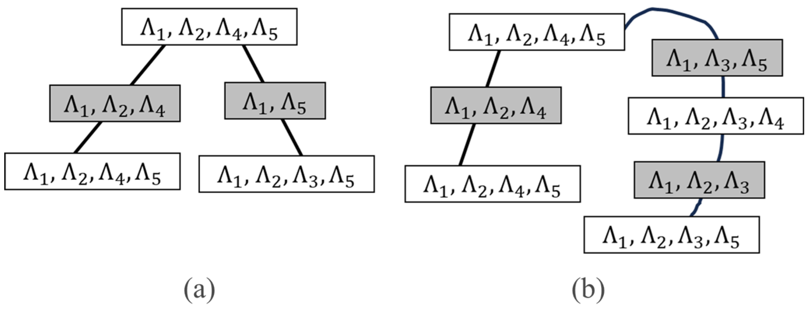
The reason for running Algorithm 3 twice is that after the first run, it is possible for a situation to arise where one side of the graph (see Figure 3a) satisfies the t-cherry property, while the other side does not. In Figure 3b, an additional cluster has been inserted between the two original clusters to form a t-cherry junction tree.

It can be seen that the algorithm is based on a greedy strategy to find the largest weight rather than using an exhaustive search. Additionally, it maintains the t-cherry property, which contains the optimal solution. This significantly reduces training time, which was proved in our previous work [28].

3. Case Study of Real-World PMU Data

3.1. Experimental Setup

3.1.1. Data

In this study, we leverage real-world PMU data sourced from the Western Interconnection segment of the continental U.S. transmission grid. The dataset comprises measurement data obtained from 23 PMU streams spanning a two-year timeframe from 2016 to 2017. These PMUs operate at a sampling rate of 60 samples per second, allowing us to capture fine-grained information. The measurements used in our experimental setup encompass key features, including the voltage magnitude of the positive sequence, the current magnitude of the positive sequence, the frequency, and the rate of change of frequency (ROCOF). Additionally, we are equipped with comprehensive event logs spanning this two-year period. These logs furnish vital details such as the event’s start timestamp, end timestamp, event type, event cause, and a descriptive explanation of the event’s nature.

In the experiments, 3866 events in the event logs are used, including 2499 line events (64.7%), 919 transformer events (23.8%), and 448 frequency events (11.5%). The events in each month are randomly split into a training set (3087 events) and a testing set (779 events) in order to ensure that the events across the entire year are fairly distributed between the training set and the testing set. For the training data, we begin by preserving labels for 5% of the samples, while the remaining training data are treated as unlabeled. To evaluate the performance of the proposed weakly supervised event classification method, we assess both label estimation accuracy and conduct a fair comparison with semi-supervised learning approaches. The event classification performance was evaluated over 20 runs. In each run, labeled training samples were randomly selected while maintaining the original class distribution across the three event types: line events (64.7%), transformer events (23.8%), and frequency events (11.5%).

Based on our previous studies [4,26], we found that the combination of features—ROCOF down area, current up area, and the change segment of voltage—is important for identifying frequency events. These features can inform the design of labeling functions that incorporate domain knowledge.

3.1.2. Evaluation Metrics

Four metrics are used to evaluate the classification performance, i.e., accuracy (ACC), precision (PRE), recall (REC), and F1 score, which are defined as follows:

$$\begin{array}{cc}\hfill \mathrm{ACC}& =(\mathrm{TP}+\mathrm{TN})/(\mathrm{TP}+\mathrm{TN}+\mathrm{FP}+\mathrm{FN}),\hfill \\ \hfill \mathrm{PRE}& =\mathrm{TP}/(\mathrm{TP}+\mathrm{FP}),\hfill \\ \hfill \mathrm{REC}& =\mathrm{TP}/(\mathrm{TP}+\mathrm{FN}),\hfill \\ \hfill \mathrm{F}1& =2\times (\mathrm{PRE}\times \mathrm{REC})/(\mathrm{PRE}+\mathrm{REC}),\hfill \end{array}$$

where TP (i.e., True Positive) and TN (i.e., True Negative) denote the number of positive and negative instances that are correctly classified, respectively. FP (i.e., False Positive) and FN (i.e., False Negative) denote the number of misclassified negative and positive instances, respectively.

3.2. Label Estimation Accuracy

The accuracy of the estimated labels using weakly supervised learning (i.e., Snorkel [26], second-order, third-order and fourth-order t-cherry junction tree) and the semi-supervised (i.e., self-training and label-spreading models) with the labeling rate from 5% (i.e., 154 labeled events) to 15% (i.e., 463 labeled events) over 20 runs are compared and shown in

Table 2. The accuracy of the estimated labels under different labeled training data rates (5–15%). Bold indicates the optimal values.

Labeled Data Rate (%)	Snorkel	SelfTrain	LabelSpread	2 Order	3 Order	4 Order
5	$56.3\pm 4.1$	$69.1\pm 1.6$	$65.7\pm 0.2$	$68.6\pm 0.9$	$67.9\pm 1.3$	$\mathbf{70}.\mathbf{1}\pm 1.4$
6	$58.1\pm 1.7$	$68.5\pm 1.3$	$66.0\pm 0.1$	$\mathbf{69}.\mathbf{0}\pm 0.7$	$67.4\pm 0.9$	$68.8\pm 1.7$
7	$59.7\pm 1.2$	$69.7\pm 1.1$	$66.2\pm 0.2$	$69.6\pm 1.0$	$67.8\pm 1.2$	$\mathbf{69}.\mathbf{9}\pm 1.4$
8	$57.6\pm 1.5$	$70.6\pm 1.5$	$66.5\pm 0.2$	$70.4\pm 0.5$	$69.3\pm 1.5$	$\mathbf{70}.\mathbf{8}\pm 1.0$
9	$59.9\pm 2.9$	$70.9\pm 1.5$	$66.6\pm 0.3$	$\mathbf{71}.\mathbf{1}\pm 1.3$	$68.6\pm 1.4$	$71.0\pm 2.8$
10	$62.2\pm 2.0$	$71.5\pm 0.8$	$66.7\pm 0.2$	$\mathbf{71}.\mathbf{7}\pm 1.3$	$68.9\pm 1.3$	$70.7\pm 1.4$
11	$61.4\pm 2.7$	$71.0\pm 0.9$	$67.0\pm 0.4$	$71.3\pm 1.4$	$69.5\pm 2.1$	$\mathbf{71}.\mathbf{6}\pm 1.5$
12	$63.6\pm 2.3$	$73.2\pm 1.7$	$67.4\pm 0.4$	$\mathbf{73}.\mathbf{4}\pm 1.6$	$72.1\pm 2.6$	$73.0\pm 1.5$
13	$64.3\pm 2.4$	$73.3\pm 1.9$	$67.6\pm 0.6$	$\mathbf{73}.\mathbf{9}\pm 1.6$	$74.7\pm 1.2$	$73.4\pm 3.0$
14	$63.9\pm 1.9$	$73.4\pm 0.8$	$67.7\pm 0.3$	$\mathbf{74}.\mathbf{0}\pm 1.4$	$73.0\pm 3.9$	$72.9\pm 4.1$
15	$64.2\pm 1.8$	$73.9\pm 1.1$	$67.9\pm 0.3$	$74.6\pm 1.0$	$74.9\pm 0.8$	$\mathbf{75}.\mathbf{0}\pm 0.7$

(each cell shows the accuracy value of average ± one standard deviation). In the context of semi-supervised learning, specifically self-training learning, various classifiers can be selected. We conducted a comparative analysis of several classifiers, including Decision Tree, Multinomial Naive Bayes (NB), Support Vector Classifier (SVC), Logistic Regression, and K-Nearest Neighbor (KNN). The results indicated that the semi-supervised Decision Tree outperformed the others. During each run, hyperparameter tuning is performed to measure the maximum depth of the tree, minimum number of samples required to split a node, minimum number of samples required at a leaf node, minimum weighted fraction of the sum total of weights required at a leaf node, and maximum number of leaf nodes. Since we run 20 times and the training data introduced each time contain randomness, the results vary with each execution. These parameters are difficult to record consistently for comparison. Therefore, decision tree models for self-training after hyperparameter tuning are used.

It is observed that our method outperforms the semi-supervised models. Compared with the semi-supervised models, the proposed weakly supervised learning can easily incorporate the domain knowledge using different LFs and thereby enhance the accuracy of the estimated labels. As evident from the results, the outcomes of the t-cherry junction trees are consistently better than those of the semi-supervised learning models.

Running times were measured under identical experimental conditions on a Windows 10 Pro 64-bit operating system with an x64-based Intel(R) i7-11700 CPU @ 2.50 GHz and 32.0 GB of RAM. The average running times for the 2nd, 3rd, and 4th-order t-cherry junction tree models were approximately 5, 12, and 22 seconds, respectively, demonstrating the method’s suitability for large-scale deployment. The code is available in GitHub [30].

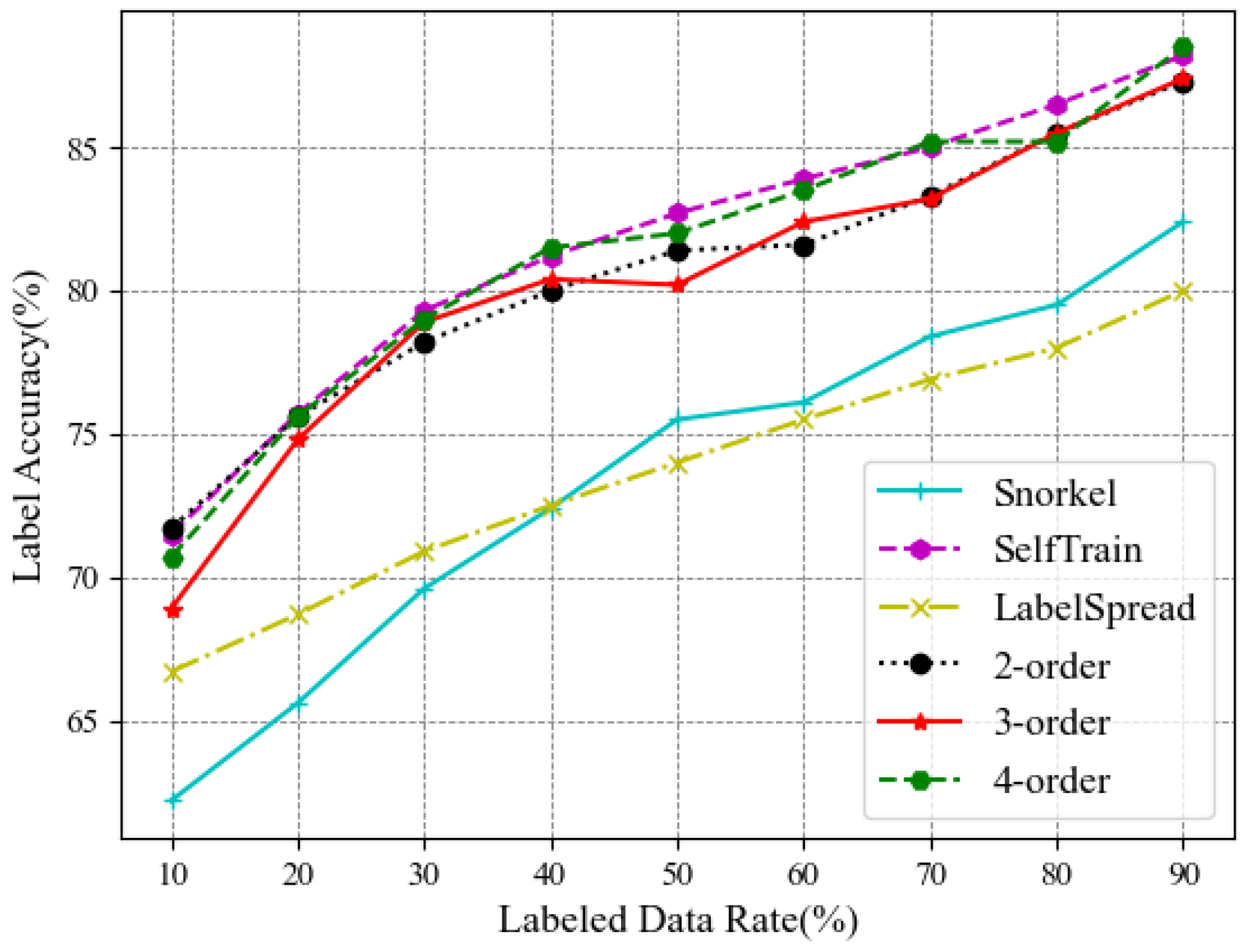
We further compare the classification performance under different labeled data rates at a large scale. As shown in Figure 4, all models increase as the labeling data rate increases, and after exceeding 20%, the performance of the SelfTrain and t-cherry junction tree models is comparable.

Remark 1.

The experiment is set in a scenario with the same event distribution but different numbers of training datasets. Here, it can be seen that below 15%, our system performs significantly better than semi-supervised learning models. If the condition of having the same event distribution is not met, semi-supervised learning cannot utilize labeling functions based on domain knowledge, rendering the model unable to make judgments on unseen new events. Therefore, semi-supervised learning completely fails to operate in situations with low data volume and a lack of labels for certain classes.

3.3. Event Classification Performance

Table 3. The accuracy of the testing data under different labeled training data rates (5–15%).Bold indicates the optimal values.

Labeled Data Rate (%)	Snorkel	SelfTrain	LabelSpread	2 Order	3 Order	4 Order
5	$56.3\pm 4.1$	$69.1\pm 1.6$	$65.7\pm 0.2$	$68.6\pm 0.9$	$67.9\pm 1.3$	$\mathbf{70}.\mathbf{1}\pm 1.4$
6	$58.1\pm 1.7$	$68.5\pm 1.3$	$66.0\pm 0.1$	$\mathbf{69}.\mathbf{0}\pm 0.7$	$67.4\pm 0.9$	$68.8\pm 1.7$
7	$59.7\pm 1.2$	$69.7\pm 1.1$	$66.2\pm 0.2$	$69.6\pm 1.0$	$67.8\pm 1.2$	$\mathbf{69}.\mathbf{9}\pm 1.4$
8	$57.6\pm 1.5$	$70.6\pm 1.5$	$66.5\pm 0.2$	$70.4\pm 0.5$	$69.3\pm 1.5$	$\mathbf{70}.\mathbf{8}\pm 1.0$
9	$59.9\pm 2.9$	$70.9\pm 1.5$	$66.6\pm 0.3$	$\mathbf{71}.\mathbf{1}\pm 1.3$	$68.6\pm 1.4$	$71.0\pm 2.8$
10	$62.2\pm 2.0$	$71.5\pm 0.8$	$66.7\pm 0.2$	$\mathbf{71}.\mathbf{7}\pm 1.3$	$68.9\pm 1.3$	$70.7\pm 1.4$
11	$61.4\pm 2.7$	$71.0\pm 0.9$	$67.0\pm 0.4$	$71.3\pm 1.4$	$69.5\pm 2.1$	$\mathbf{71}.\mathbf{6}\pm 1.5$
12	$63.6\pm 2.3$	$73.2\pm 1.7$	$67.4\pm 0.4$	$\mathbf{73}.\mathbf{4}\pm 1.6$	$72.1\pm 2.6$	$73.0\pm 1.5$
13	$64.3\pm 2.4$	$73.3\pm 1.9$	$67.6\pm 0.6$	$\mathbf{73}.\mathbf{9}\pm 1.6$	$74.7\pm 1.2$	$73.4\pm 3.0$
14	$63.9\pm 1.9$	$73.4\pm 0.8$	$67.7\pm 0.3$	$\mathbf{74}.\mathbf{0}\pm 1.4$	$73.0\pm 3.9$	$72.9\pm 4.1$
15	$64.2\pm 1.8$	$73.9\pm 1.1$	$67.9\pm 0.3$	$74.6\pm 1.0$	$74.9\pm 0.8$	$\mathbf{75}.\mathbf{0}\pm 0.7$

compares the average performance of the 2nd, 3rd, and 4th-order t-cherry junction tree models using Random Forest and various semi-supervised approaches. The t-cherry junction tree model, trained in a weakly supervised manner, consistently outperforms the two semi-supervised baselines—Self-Training and Label Spreading. Across all settings, the t-cherry junction tree achieves superior performance compared to the other models.

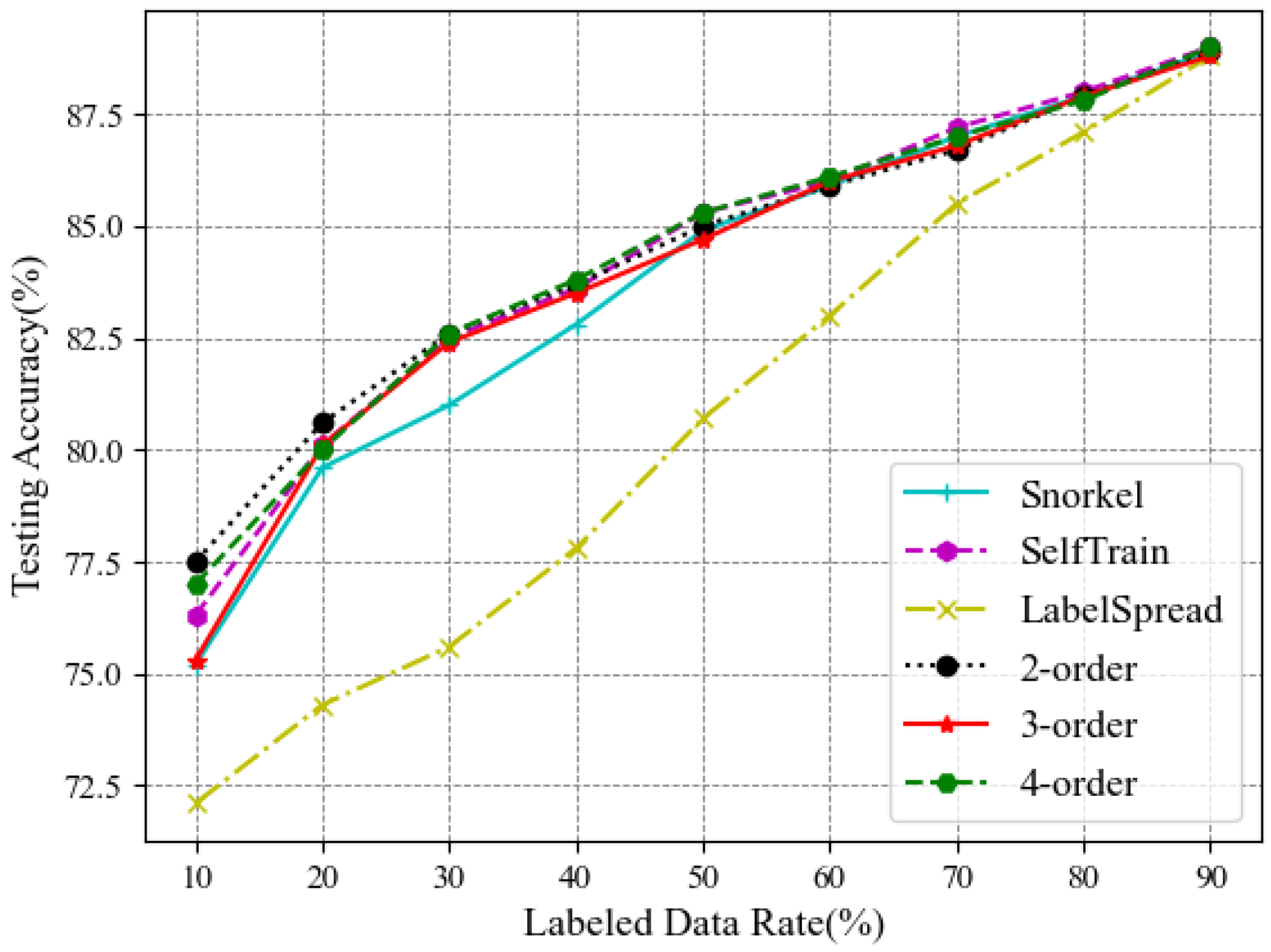
We further evaluate classification performance at varying labeled data rates. As shown in Figure 5, the performance of all models improves as the proportion of labeled data increases. Notably, once the labeling rate exceeds 20%, the performance of the Self-Training and t-cherry junction tree models becomes comparable.

Since we observed that the 4th-order model performed relatively well when the training data comprised only 5%, we conducted a t-test in

Table 4. The t-test results comparing the average values of the 4th-order model and other models (5% labeled data) across 20 runs.

Comparison	t Value	p Value	Significant (0.05)
4th-order vs. Snorkel	9.83	<0.0001	Yes
4th-order vs. SelfTrain	1.48	0.16	No
4th-order vs. LabelSpread	9.87	<0.0001	Yes
4th-order vs. 2nd-order	2.79	0.011	Yes
4th-order vs. 3rd-order	3.65	0.002	Yes

. Under the condition of using only 5% labeled data, we performed an independent samples t-test between the 4th-order model and the other methods to evaluate the performance differences between the approaches. The results indicate that the comparisons between the 4th-order and the Snorkel, LabelSpread, 2nd-order, and 3rd-order models all show significant differences (p < 0.05) with particularly notable differences compared to Snorkel and LabelSpread (p < 0.0001). This suggests that the 4th-order model has a clear performance advantage in low-label scenarios. Additionally, the difference between the 4th-order model and the SelfTrain model is not significant (p = 0.16), indicating that their performances are similar. Overall, these results demonstrate that the proposed 4th-order model can stably improve classification performance under weak supervision and exhibits statistically significant superiority over most baseline methods.

Discussion: From a computational complexity perspective, the second-order approach is definitely faster in terms of calculation speed. Based on our previous algorithm analysis, we found that the running time is actually related to the number of clusters. Generally speaking, when the number of labeling functions is fixed, the number of clusters in the second-order approach is relatively smaller. Indeed, higher-order approaches (such as the fourth-order approach in our case) may yield better performance, but they also impose a heavier computational burden. Therefore, our work mainly focuses on reducing the computational complexity of higher-order approaches, which is also an important contribution of our work.

3.4. Impact of Labeling Function Choice

In our initial experiments, we utilized a predefined set of labeling functions (LFs), as detailed in Table 1. To further assess the robustness of our method across different labeling strategies, we performed additional experiments with alternative LF configurations. To ensure the generalizability of our findings, the current section deliberately avoids incorporating domain-specific knowledge when designing new labeling functions, as there are no unseen events. Subsequently, in Section 3.5, we demonstrate how domain-informed labeling functions can enhance model performance when applied to unseen events.

For this study, we introduce an alternative labeling function configuration, referred to as Labeling Function Combination 1-5 (LFC1-5), which employs widely used machine learning models—Random Forest (RF), Logistic Regression (LR), K-Nearest Neighbor (KNN), and Support Vector Machine (SVM)—to generate features based on voltage and rate of change of frequency (ROCOF) signals. These configurations are summarized in

Table 5. Different combinations of labeling functions, where V represents the voltage magnitude, I represents the current magnitude, and R represents the ROCOF signal.

	LFC1	LFC2	LFC3	LFC4	LFC5
${\lambda }_1$	V-RF	V-RF	I-RF	V-RF	I-RF
${\lambda }_2$	V-LR	V-LR	I-LR	V-SVM	I-LR
${\lambda }_3$	V-KNN	V-KNN	I-KNN	V-KNN	I-SVM
${\lambda }_4$	V-GBDT	V-SVM	I-SVM	V-GBDT	I-GBDT
${\lambda }_5$	R-RF	R-RF	R-RF	R-RF	R-RF
${\lambda }_6$	R-LR	R-LR	R-LR	R-SVM	R-LR
${\lambda }_7$	R-KNN	R-KNN	R-KNN	R-KNN	R-SVM
${\lambda }_8$	R-GBDT	R-SVM	R-SVM	R-GBDT	R-GBDT

, which presents labeling functions derived from ROCOF (R), voltage (V), and current (I) magnitude signals. For example, V-RF represents the labeling function derived from voltage signals using the Random Forest algorithm.

The results from

Table 6. The accuracy of the estimated labels by 2nd-order t-cherry junction tree under different labeled training data rates (5–15%). Bold indicates the optimal values.

Labeled Data Rate (%)	LFC1	LFC2	LFC3	LFC4	LFC5
5	$\mathbf{68}.\mathbf{6}\pm 0.9$	$66.0\pm 3.1$	$62.4\pm 2.7$	$67.6\pm 1.7$	$68.0\pm 1.7$
6	$\mathbf{69}.\mathbf{0}\pm 0.7$	$67.1\pm 1.8$	$62.6\pm 1.8$	$67.4\pm 1.3$	$67.6\pm 1.1$
7	$\mathbf{69}.\mathbf{6}\pm 1.0$	$69.4\pm 1.1$	$64.9\pm 1.5$	$68.6\pm 1.8$	$68.9\pm 1.9$
8	$\mathbf{70}.\mathbf{4}\pm 0.5$	$69.6\pm 1.0$	$64.3\pm 2.3$	$66.4\pm 5.6$	$68.5\pm 3.5$
9	$\mathbf{71}.\mathbf{1}\pm 1.3$	$69.5\pm 2.5$	$64.6\pm 1.8$	$70.4\pm 1.1$	$70.3\pm 1.0$
10	$\mathbf{71}.\mathbf{7}\pm 1.3$	$70.7\pm 1.0$	$66.1\pm 1.5$	$70.8\pm 1.1$	$70.8\pm 1.1$
11	$\mathbf{71}.\mathbf{3}\pm 1.4$	$70.5\pm 2.3$	$66.1\pm 1.4$	$68.7\pm 4.7$	$69.9\pm 4.0$
12	$\mathbf{73}.\mathbf{4}\pm 1.6$	$71.2\pm 0.6$	$66.0\pm 3.5$	$71.1\pm 0.7$	$71.1\pm 0.7$
13	$\mathbf{73}.\mathbf{9}\pm 1.6$	$71.8\pm 0.9$	$66.9\pm 1.6$	$71.0\pm 4.2$	$72.0\pm 0.8$
14	$\mathbf{74}.\mathbf{0}\pm 1.4$	$72.1\pm 0.8$	$67.8\pm 1.5$	$72.4\pm 0.7$	$72.2\pm 0.7$
15	$\mathbf{74}.\mathbf{6}\pm 1.0$	$72.5\pm 1.2$	$67.3\pm 2.1$	$72.3\pm 0.8$	$72.3\pm 1.2$

,

Table 7. The accuracy of the testing data by 2nd-order t-cherry junction tree under different labeled training data rates (5–15%). Bold indicates the optimal values.

Labeled Data Rate (%)	LFC1	LFC2	LFC3	LFC4	LFC5
5	$\mathbf{75}.\mathbf{4}\pm 0.8$	$73.9\pm 2.2$	$71.6\pm 1.9$	$74.9\pm 1.0$	$75.1\pm 1.1$
6	$\mathbf{75}.\mathbf{8}\pm 1.9$	$74.2\pm 1.5$	$71.2\pm 1.3$	$74.3\pm 1.5$	$74.7\pm 1.4$
7	$75.7\pm 0.9$	$\mathbf{76}.\mathbf{6}\pm 1.0$	$73.0\pm 1.4$	$75.8\pm 1.9$	$75.7\pm 2.0$
8	$\mathbf{76}.\mathbf{9}\pm 1.1$	$76.4\pm 1.0$	$72.7\pm 1.7$	$74.4\pm 3.8$	$75.2\pm 2.8$
9	$\mathbf{77}.\mathbf{4}\pm 1.7$	$75.9\pm 3.0$	$72.8\pm 1.2$	$\mathbf{77}.\mathbf{4}\pm 1.1$	$77.2\pm 1.3$
10	$77.5\pm 1.0$	$77.6\pm 0.6$	$74.1\pm 1.3$	$\mathbf{77}.\mathbf{8}\pm 0.7$	$77.6\pm 0.8$
11	$\mathbf{77}.\mathbf{6}\pm 0.8$	$76.8\pm 2.5$	$74.8\pm 1.0$	$76.6\pm 3.2$	$77.1\pm 3.3$
12	$78.3\pm 1.0$	$\mathbf{78}.\mathbf{4}\pm 1.1$	$74.1\pm 3.5$	$78.3\pm 0.9$	$77.9\pm 0.7$
13	$78.6\pm 1.2$	$79.2\pm 0.9$	$75.8\pm 1.5$	$78.4\pm 3.0$	$\mathbf{79}.\mathbf{5}\pm 0.6$
14	$79.2\pm 0.9$	$79.9\pm 0.7$	$76.8\pm 1.1$	$\mathbf{80}.\mathbf{0}\pm 0.9$	$79.7\pm 0.7$
15	$79.4\pm 1.0$	$\mathbf{80}.\mathbf{1}\pm 1.6$	$76.7\pm 1.7$	$79.5\pm 1.2$	$79.6\pm 1.3$

,

Table 8. The accuracy of the estimated labels by 3rd-order t-cherry junction tree under different labeled training data rates (5–15%). Bold indicates the optimal values.

Labeled Data Rate (%)	LFC1	LFC2	LFC3	LFC4	LFC5
5	$\mathbf{67}.\mathbf{9}\pm 1.3$	$66.1\pm 3.7$	$62.8\pm 2.9$	$64.5\pm 2.3$	$66.1\pm 2.8$
6	$67.4\pm 0.9$	$\mathbf{67}.\mathbf{5}\pm 0.9$	$63.0\pm 2.2$	$66.1\pm 1.6$	$64.5\pm 3.2$
7	$67.8\pm 1.2$	$\mathbf{69}.\mathbf{1}\pm 1.9$	$64.5\pm 0.9$	$66.8\pm 1.8$	$67.8\pm 2.2$
8	$\mathbf{69}.\mathbf{3}\pm 1.5$	$69.0\pm 2.0$	$64.4\pm 2.2$	$64.5\pm 6.0$	$66.4\pm 3.4$
9	$68.6\pm 1.4$	$\mathbf{70}.\mathbf{2}\pm 1.0$	$64.5\pm 2.2$	$68.6\pm 1.9$	$67.7\pm 2.4$
10	$\mathbf{68}.\mathbf{9}\pm 1.3$	$68.4\pm 3.8$	$64.5\pm 2.4$	$67.9\pm 2.5$	$66.9\pm 2.1$
11	$\mathbf{69}.\mathbf{5}\pm 2.1$	$\mathbf{69}.\mathbf{5}\pm 3.3$	$65.4\pm 2.9$	$66.7\pm 4.8$	$67.7\pm 4.1$
12	$\mathbf{72}.\mathbf{1}\pm 2.6$	$70.5\pm 2.3$	$66.9\pm 3.7$	$69.3\pm 1.3$	$68.0\pm 1.3$
13	$\mathbf{74}.\mathbf{7}\pm 1.2$	$72.0\pm 1.0$	$66.9\pm 2.2$	$68.3\pm 3.9$	$70.6\pm 1.8$
14	$\mathbf{73}.\mathbf{0}\pm 3.9$	$72.1\pm 0.8$	$67.4\pm 2.5$	$70.2\pm 1.6$	$70.0\pm 1.8$
15	$\mathbf{74}.\mathbf{9}\pm 0.8$	$71.2\pm 3.2$	$68.2\pm 2.0$	$69.7\pm 2.0$	$69.7\pm 2.0$

,

Table 9. The accuracy of the testing data by 3rd-order t-cherry junction tree under different labeled training data rates (5–15%). Bold indicates the optimal values.

Labeled Data Rate (%)	LFC1	LFC2	LFC3	LFC4	LFC5
5	$\mathbf{75}.\mathbf{0}\pm 0.7$	$73.6\pm 3.0$	$71.7\pm 2.1$	$72.8\pm 1.3$	$74.2\pm 1.7$
6	$\mathbf{74}.\mathbf{9}\pm 1.1$	$74.3\pm 1.3$	$71.6\pm 1.4$	$73.6\pm 1.6$	$73.1\pm 2.5$
7	$74.9\pm 0.7$	$\mathbf{76}.\mathbf{3}\pm 1.5$	$72.6\pm 1.0$	$74.6\pm 1.5$	$75.0\pm 1.5$
8	$75.5\pm 0.7$	$\mathbf{76}.\mathbf{0}\pm 1.9$	$73.1\pm 1.5$	$73.4\pm 4.3$	$74.2\pm 2.5$
9	$75.8\pm 0.7$	$\mathbf{76}.\mathbf{5}\pm 2.6$	$73.1\pm 1.8$	$76.2\pm 1.2$	$55.9\pm 1.6$
10	$75.3\pm 0.8$	$75.9\pm 3.3$	$73.2\pm 2.2$	$\mathbf{76}.\mathbf{0}\pm 1.4$	$75.6\pm 1.2$
11	$\mathbf{76}.\mathbf{7}\pm 1.2$	$76.3\pm 2.8$	$74.1\pm 2.0$	$75.5\pm 3.6$	$76.1\pm 2.8$
12	$77.5\pm 1.2$	$\mathbf{77}.\mathbf{8}\pm 2.0$	$74.2\pm 4.0$	$77.2\pm 0.9$	$76.2\pm 1.4$
13	$78.9\pm 1.1$	$\mathbf{79}.\mathbf{3}\pm 0.8$	$75.9\pm 1.8$	$77.0\pm 2.9$	$78.4\pm 1.3$
14	$78.7\pm 1.9$	$\mathbf{80}.\mathbf{0}\pm 0.7$	$76.5\pm 1.7$	$78.7\pm 1.3$	$78.4\pm 1.4$
15	$\mathbf{79}.\mathbf{1}\pm 1.2$	$79.0\pm 2.3$	$77.4\pm 2.0$	$78.3\pm 1.5$	$78.3\pm 1.7$

,

Table 10. The accuracy of the estimated labels by 4th-order t-cherry junction tree under different labeled training data rates (5–15%). Bold indicates the optimal values.

Labeled Data Rate (%)	LFC1	LFC2	LFC3	LFC4	LFC5
5	$\mathbf{70}.\mathbf{1}\pm 1.4$	$67.1\pm 2.1$	$62.2\pm 2.7$	$66.5\pm 2.0$	$64.3\pm 2.4$
6	$\mathbf{68}.\mathbf{8}\pm 1.7$	$67.6\pm 1.2$	$61.1\pm 4.0$	$64.3\pm 1.5$	$64.6\pm 2.7$
7	$\mathbf{69}.\mathbf{9}\pm 1.4$	$68.3\pm 2.8$	$64.4\pm 1.3$	$66.7\pm 2.0$	$66.5\pm 2.5$
8	$\mathbf{70}.\mathbf{8}\pm 1.0$	$68.4\pm 2.2$	$64.7\pm 2.6$	$64.3\pm 6.2$	$66.1\pm 3.5$
9	$\mathbf{71}.\mathbf{0}\pm 2.8$	$69.4\pm 2.6$	$64.1\pm 4.0$	$68.4\pm 1.6$	$67.7\pm 2.3$
10	$\mathbf{70}.\mathbf{7}\pm 1.4$	$68.9\pm 3.8$	$62.8\pm 2.6$	$68.4\pm 2.0$	$68.1\pm 1.2$
11	$\mathbf{71}.\mathbf{6}\pm 1.5$	$70.2\pm 3.1$	$66.2\pm 1.3$	$66.6\pm 4.9$	$68.2\pm 4.1$
12	$\mathbf{73}.\mathbf{0}\pm 1.5$	$70.1\pm 2.8$	$65.3\pm 3.3$	$68.1\pm 1.8$	$68.8\pm 0.9$
13	$\mathbf{73}.\mathbf{4}\pm 3.0$	$70.4\pm 2.8$	$66.7\pm 1.6$	$69.2\pm 4.3$	$70.8\pm 1.9$
14	$\mathbf{72}.\mathbf{9}\pm 4.1$	$70.9\pm 2.3$	$67.1\pm 3.0$	$70.4\pm 1.6$	$70.3\pm 0.8$
15	$\mathbf{75}.\mathbf{0}\pm 0.7$	$71.9\pm 2.3$	$66.4\pm 4.1$	$69.9\pm 2.2$	$71.4\pm 2.0$

and

Table 11. The accuracy of the testing data by 4th-order t-cherry junction tree under different labeled training data rates (5–15%). Bold indicates the optimal values.

Labeled Data Rate (%)	LFC1	LFC2	LFC3	LFC4	LFC5
5	$\mathbf{76}.\mathbf{4}\pm 1.0$	$74.4\pm 1.6$	$71.3\pm 2.2$	$74.2\pm 1.0$	$72.9\pm 1.6$
6	$\mathbf{75}.\mathbf{7}\pm 1.2$	$74.4\pm 1.3$	$70.3\pm 2.9$	$72.1\pm 1.7$	$73.0\pm 1.9$
7	$\mathbf{75}.\mathbf{8}\pm 1.0$	$\mathbf{75}.\mathbf{8}\pm 1.9$	$72.8\pm 1.3$	$74.7\pm 1.3$	$74.3\pm 1.9$
8	$\mathbf{76}.\mathbf{2}\pm 0.7$	$75.6\pm 1.7$	$73.2\pm 2.0$	$73.1\pm 4.4$	$73.9\pm 2.2$
9	$\mathbf{77}.\mathbf{6}\pm 2.0$	$76.1\pm 2.9$	$72.8\pm 2.7$	$76.4\pm 0.9$	$75.7\pm 1.4$
10	$\mathbf{77}.\mathbf{0}\pm 1.6$	$76.1\pm 2.5$	$71.8\pm 2.6$	$76.4\pm 1.4$	$76.1\pm 1.7$
11	$\mathbf{77}.\mathbf{8}\pm 0.8$	$76.9\pm 2.9$	$74.8\pm 1.3$	$75.2\pm 3.8$	$76.2\pm 3.3$
12	$\mathbf{77}.\mathbf{7}\pm 1.5$	$76.8\pm 2.8$	$73.5\pm 3.6$	$76.3\pm 1.7$	$76.6\pm 0.9$
13	$\mathbf{78}.\mathbf{2}\pm 2.1$	$78.1\pm 2.2$	$75.7\pm 1.6$	$77.7\pm 3.2$	$78.8\pm 1.5$
14	$78.3\pm 2.4$	$\mathbf{79}.\mathbf{3}\pm 1.2$	$76.7\pm 2.3$	$78.8\pm 1.6$	$78.6\pm 0.8$
15	$79.1\pm 1.3$	$\mathbf{79}.\mathbf{5}\pm 1.8$	$76.4\pm 3.0$	$78.2\pm 1.6$	$\mathbf{79}.\mathbf{5}\pm 1.1$

demonstrate that labeling functions based on current signals exhibit inferior performance compared to those utilizing voltage signals. Consequently, we evaluate the impact of replacing the machine learning models used to construct the labeling functions while retaining voltage and ROCOF signals as the feature sources.

As shown in Table 6, the estimated labels from the 2nd-order Labeling Function Combination 1 (LFC1) consistently outperform other combinations. However, the testing results in Table 7 reveal that for training data exceeding 10%, the performance of other combinations may surpass that of LFC1. In the 3rd-order results, LFC1 and LFC2 achieve higher accuracy than other configurations. For the 4th-order results, LFC1 yields superior estimated label results, yet when the training data exceed 13%, the testing accuracy of LFC2 exceeds that of LFC1.

Notably, even in fully supervised learning scenarios (where 100% of the training dataset is correctly labeled), confusion between line events and transformer events remains likely. Thus, while the estimated label accuracy may be high, the testing accuracy may not necessarily surpass that of other combinations.

From these results, we observe that the 2nd- and 4th-order combinations consistently outperform others regardless of the specific labeling function combinations. We did not test 5th-order combinations because only eight labeling functions are available, and the number of consistent combinations per node becomes similar to that of the 3rd order. Additionally, this experiment helps verify whether the proposed approach can yield improved performance.

We also chose not to explore larger labeled data rates, as previous results (see Figure 5) suggest that beyond a 20% rate, the performance differences between labeling function combinations become relatively marginal.

3.5. Robustness on Unseen Events

We conduct a comparison between weakly supervised and semi-supervised learning paradigms by incorporating domain knowledge into our modeling framework. The experimental setup features an intentionally incomplete training dataset that lacks frequency events (containing only line and transformer events) while maintaining all three event categories in the testing data. This configuration reveals a fundamental limitation of semi-supervised approaches—their inability to recognize the missing frequency events due to complete dependence on the partial training labels. In contrast, our weakly supervised method successfully identifies these unseen events through the strategic application of domain knowledge, where predefined thresholds on specific feature values trigger assignment of the missing category.

To ensure rigorous comparison, we maintain identical test conditions while deliberately mislabeling all frequency events in the training data as line events (the majority class). The semi-supervised baseline processes this modified dataset directly, whereas our weak supervision approach employs specialized labeling functions (Table 1), replacing ${\lambda }_2$, ${\lambda }_3$, and ${\lambda }_6$ with custom functions derived from domain-specific feature analysis. This methodological distinction enables our framework to overcome the inherent limitations of conventional semi-supervised learning when handling incomplete training data.

The semi-supervised method uses this modified training set directly. In contrast, weak supervision employs labeling functions (Table 1), where we replace ${\lambda }_2$, ${\lambda }_3$, and ${\lambda }_6$ with custom functions based on domain-specific features:

• Maximum ROCOF ($Max\left(F_6^{Rof}\right)$);
• Maximum voltage drop ($Max\left(F_4^V\right)$);
• Maximum current drop ($Max\left(F_3^I\right)$).

While precise thresholds for these functions remain unknown, we derive heuristic constraints from empirical data for the voltage, current, and ROCOF signals. Although this experiment demonstrates the framework’s capability to detect unseen events, performance optimization for such cases is not our primary focus.

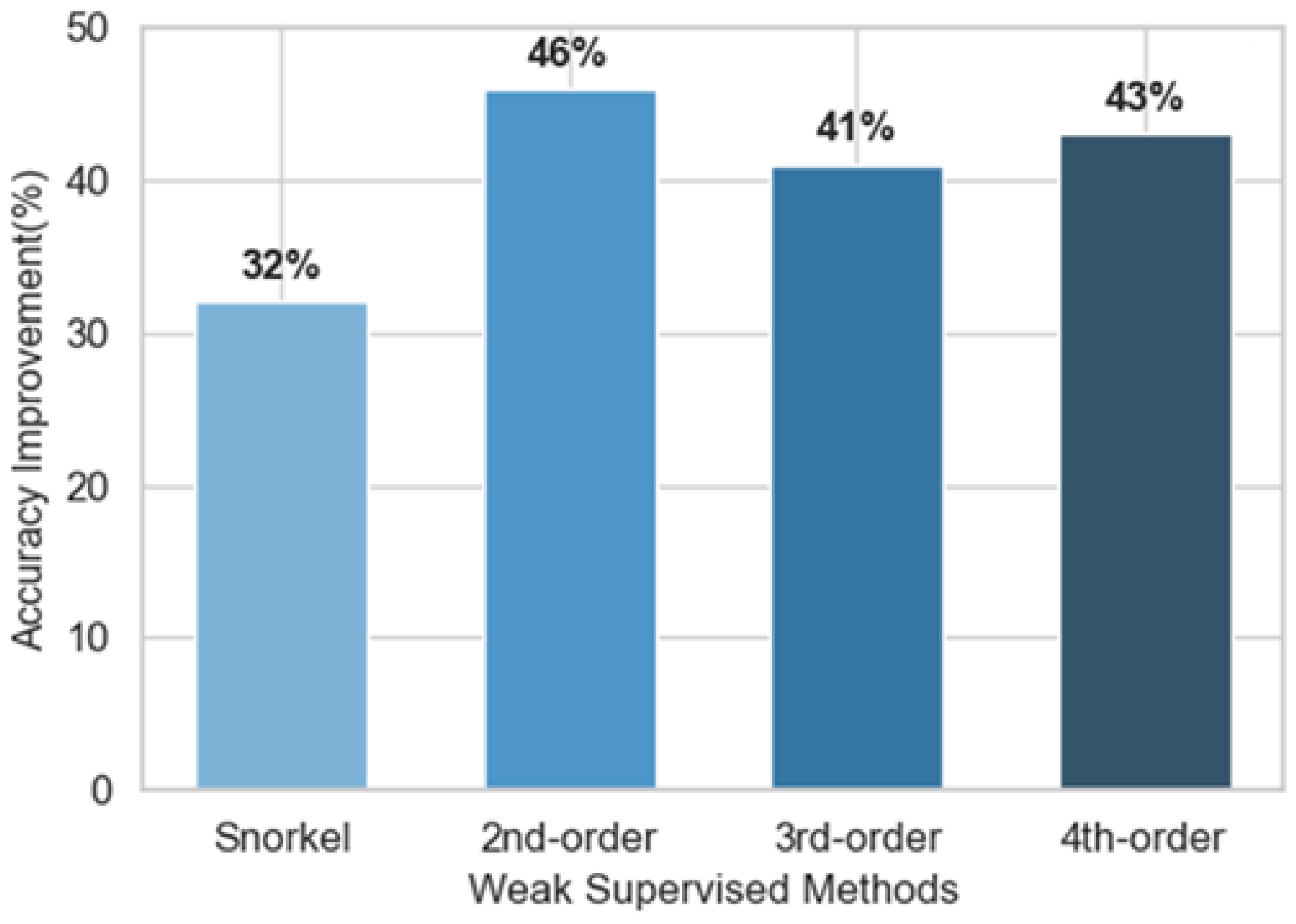
Results at 5% labeled data (consistent with our evaluation protocol, see in Figure 6) reveal striking performance disparities. Semi-supervised models fail completely in detecting unseen frequency events, whereas weakly supervised methods achieve substantial gains: Snorkel improves accuracy by 32%, while our t-cherry junction tree implementations yield even greater improvements—46% (2nd-order), 41% (3rd-order), and 43% (4th-order). Notably, the 2nd-order model’s superior performance arises from an optimal trade-off in dependency preservation: it retains the most discriminative feature relationships while mitigating approximation errors that compound in higher-order models. This insight informs PMU event classification design, demonstrating that balanced approximations can outperform more complex alternatives.

Our weakly supervised framework succeeds by leveraging imperfect yet informative domain knowledge, enabling a robust learning of latent label relationships and generalization to unseen event types—a capability absent in semi-supervised approaches.

4. Conclusions

This study explores the integration of PMU data with weakly supervised learning techniques to construct real-time automatic data labeling models for transmission grids. Our model is trained with a limited number of labeled events, which utilizes t-cherry junction tree techniques to label unlabeled events and augment the training dataset. Moreover, we devise a greedy algorithm for t-cherry junction tree generation to significantly reduce computational complexity. In comparison to existing data-driven methods, our approach achieves similar accuracy levels with only a small fraction of labeled data. Another advantage is that the model can incorporate labeling functions with domain knowledge, enabling it to classify even unseen or extremely rare events. Additionally, it demonstrates robustness against performance degradation stemming from disparities in class distribution between the training set and real-world applications. The effectiveness of our proposed method is substantiated through extensive numerical studies employing real-world PMU data.

References

1. Reuters. Spain, Portugal Switch Back On, Seek Answers After Biggest Ever Blackout; Reuters: London, UK, 2025. [Google Scholar]
2. Guo, Q.; Sun, H.; Zhang, M.; Tong, J.; Zhang, B.; Wang, B. Optimal voltage control of PJM smart transmission grid: Study, implementation, and evaluation. IEEE Trans. Smart Grid 2013, 4, 1665–1674. [Google Scholar] [CrossRef]
3. Niazazari, I.; Liu, Y.; Ghasenikhani, A.; Biswas, S.; Livani, H.; Yang, L.; Centeno, V.A. PMU-data-driven Event Classification in Power Transmission Grids. In Proceedings of the 2021 IEEE Power & Energy Society Innovative Smart Grid Technologies Conference (ISGT), Virtual, 16–18 February 2021; pp. 1–5. [Google Scholar]
4. Liu, Y.; Yang, L.; Ghasemkhani, A.; Livani, H.; Centeno, V.A.; Chen, P.Y.; Zhang, J. Robust event classification using imperfect real-world PMU data. IEEE Internet Things J. 2022, 10, 7429–7438. [Google Scholar] [CrossRef]
5. Ratner, A.; Bach, S.H.; Ehrenberg, H.; Fries, J.; Wu, S.; Ré, C. Snorkel: Rapid training data creation with weak supervision. In Proceedings of the VLDB Endowment. International Conference on Very Large Data Bases, NIH Public Access, Munich, Germany, 28 August–1 September 2017; Volume 11, p. 269. [Google Scholar]
6. Foggo, B.; Yamashita, K.; Yu, N. pmuBAGE: The Benchmarking Assortment of Generated PMU Data for Power System Events. IEEE Trans. Power Syst. 2023, 39, 3485–3496. [Google Scholar] [CrossRef]
7. Liu, S.; Zhao, Y.; Lin, Z.; Liu, Y.; Ding, Y.; Yang, L.; Yi, S. Data-driven event detection of power systems based on unequal-interval reduction of PMU data and local outlier factor. IEEE Trans. Smart Grid 2019, 11, 1630–1643. [Google Scholar] [CrossRef]
8. Taghipourbazargani, N.; Dasarathy, G.; Sankar, L.; Kosut, O. A machine learning framework for event identification via modal analysis of PMU data. IEEE Trans. Power Syst. 2022, 38, 4165–4176. [Google Scholar] [CrossRef]
9. Zheng, X.; Wang, B.; Kalathil, D.; Xie, L. Generative Adversarial Networks-Based Synthetic PMU Data Creation for Improved Event Classification. IEEE Open Access J. Power Energy 2021, 8, 68–76. [Google Scholar] [CrossRef]
10. Li, H.; Ma, Z.; Weng, Y. A transfer learning framework for power system event identification. IEEE Trans. Power Syst. 2022, 37, 4424–4435. [Google Scholar] [CrossRef]
11. Bin Akter, S.; Sarkar Pias, T.; Rahman Deeba, S.; Hossain, J.; Abdur Rahman, H. Ensemble learning based transmission line fault classification using phasor measurement unit (PMU) data with explainable AI (XAI). PLoS ONE 2024, 19, e0295144. [Google Scholar] [CrossRef]
12. Li, H.; Ma, Z.; Weng, Y.; Blasch, E.; Santoso, S. Structural Tensor Learning for Event Identification with Limited Labels. IEEE Trans. Power Syst. 2022, 38, 5314–5328. [Google Scholar] [CrossRef]
13. Dahal, O.P.; Brahma, S.M.; Cao, H. Comprehensive clustering of disturbance events recorded by phasor measurement units. IEEE Trans. Power Deliv. 2013, 29, 1390–1397. [Google Scholar] [CrossRef]
14. Li, W.; Wang, M.; Chow, J.H. Fast event identification through subspace characterization of PMU data in power systems. In Proceedings of the 2017 IEEE Power & Energy Society General Meeting, Chicago, IL, USA, 16–20 July 2017; pp. 1–5. [Google Scholar]
15. Chen, Y.; Xie, L.; Kumar, P.R. Power system event classification via dimensionality reduction of synchrophasor data. In Proceedings of the 2014 IEEE 8th Sensor Array and Multichannel Signal Processing Workshop (SAM), A Coruña, Spain, 22–25 June 2014; pp. 57–60. [Google Scholar]
16. Li, H.; Weng, Y.; Farantatos, E.; Patel, M. An unsupervised learning framework for event detection, type identification and localization using pmus without any historical labels. In Proceedings of the 2019 IEEE Power & Energy Society General Meeting (PESGM), Atlanta, GA, USA, 4–8 August 2019; pp. 1–5. [Google Scholar]
17. Senaratne, D.; Kim, J.; Cotilla-Sanchez, E. Spatio-Temporal Frequency Domain Analysis of PMU Data for Unsupervised Event Detection. In Proceedings of the 2021 IEEE Power & Energy Society Innovative Smart Grid Technologies Conference (ISGT), Virtual, 16–18 February 2021; pp. 1–5. [Google Scholar]
18. Cui, Q.; Weng, Y. Enhance High Impedance Fault Detection and Location Accuracy via Micro PMUs. IEEE Trans. Smart Grid 2019, 11, 797–809. [Google Scholar] [CrossRef]
19. Li, H.; Weng, Y.; Farantatos, E.; Patel, M. A hybrid machine learning framework for enhancing pmu-based event identification with limited labels. In Proceedings of the 2019 International Conference on Smart Grid Synchronized Measurements and Analytics (SGSMA), College Station, TX, USA, 21–23 May 2019; pp. 1–8. [Google Scholar]
20. Zhu, L.; Hill, D.J.; Lu, C. Auto-Starting Semisupervised-Learning-Based Identification of Synchrophasor Data Anomalies. IEEE Internet Things J. 2022, 9, 13651–13663. [Google Scholar] [CrossRef]
21. Zhou, Y.; Arghandeh, R.; Spanos, C.J. Partial knowledge data-driven event detection for power distribution networks. IEEE Trans. Smart Grid 2017, 9, 5152–5162. [Google Scholar] [CrossRef]
22. Farajzadeh-Zanjani, M.; Hallaji, E.; Razavi-Far, R.; Saif, M.; Parvania, M. Adversarial semi-supervised learning for diagnosing faults and attacks in power grids. IEEE Trans. Smart Grid 2021, 12, 3468–3478. [Google Scholar] [CrossRef]
23. Yuan, Y.; Wang, Y.; Wang, Z. A Data-driven Framework for Power System Event Type Identification via Safe Semi-supervised Techniques. IEEE Trans. Power Syst. 2023, 39, 1460–1471. [Google Scholar] [CrossRef]
24. Yang, F.; Ling, Z.; Zhang, Y.; He, X.; Ai, Q.; Qiu, R.C. Event Detection, Localization, and Classification Based on Semi-Supervised Learning in Power Grids. IEEE Trans. Power Syst. 2022, 38, 4080–4094. [Google Scholar] [CrossRef]
25. Ratner, A.J.; De Sa, C.M.; Wu, S.; Selsam, D.; Ré, C. Data programming: Creating large training sets, quickly. In Proceedings of the 30th Conference on Neural Information Processing Systems, Barcelona, Spain, 2–7 December 2016; pp. 1–9. [Google Scholar]
26. Liu, Y.; Yang, L. Weakly Supervised Event Classification Using Imperfect Real-world PMU Data with Scarce Labels. In Proceedings of the 2022 IEEE Power & Energy Society General Meeting (PESGM), Denver, CO, USA, 17–21 July 2022; pp. 1–5. [Google Scholar]
27. Szántai, T.; Kovács, E. Hypergraphs as a mean of discovering the dependence structure of a discrete multivariate probability distribution. Ann. Oper. Res. 2012, 193, 71–90. [Google Scholar] [CrossRef]
28. Proulx, B.; Zhang, J. Modeling social network relationships via t-cherry junction trees. In Proceedings of the IEEE INFOCOM 2014-IEEE Conference on Computer Communications, Toronto, ON, Canada, 27 April–2 May 2014; pp. 2229–2237. [Google Scholar]
29. Bukszár, J. Upper bounds for the probability of a union by multitrees. Adv. Appl. Probab. 2001, 33, 437–452. [Google Scholar] [CrossRef]
30. Liu, Y. Github Link. 2025. Available online: https://github.com/yunchuanliu2023/example_code (accessed on 20 October 2025).
Figure 1. The weakly supervised learning framework.
Electronics 14 04703 g001
Figure 2. Illustration of constructed features for different event types: (a) V-shape event shape; (b) narrow spike shape; (c) ramp down shape.
Electronics 14 04703 g002
Figure 3. An example of t-cherry conversion. (a) 1st time running Algorithm 3; (b) 2nd time running Algorithm 3.
Electronics 14 04703 g003
Figure 4. The accuracy of the estimated labels under different labeled training data rates (10–90%).
Electronics 14 04703 g004
Figure 5. The accuracy of the testing data under different labeled training data rates (10–90%).
Electronics 14 04703 g005
Figure 6. Accuracy improvement in terms of unseen events over semi-supervised learning.
Electronics 14 04703 g006