MIMAR-Net: Multiscale Inception-Based Manhattan Attention Residual Network and Its Application to Underwater Image Super-Resolution

Abstract

In recent years, Single-Image Super-Resolution (SISR) has gained significant attention in the geoscience and remote sensing community for its potential to improve the resolution of low-quality underwater imagery. This paper introduces MIMAR-Net (Multiscale Inception-based Manhattan Attention Residual Network), a new deep learning architecture designed to increase the spatial resolution of input color images. MIMAR-Net integrates a multiscale inception module, cascaded residue learning, and advanced attention mechanisms, such as the MaSA layer, to capture both local and global contextual information effectively. By utilizing multiscale processing and advanced attention strategies, MIMAR-Net allows us to handle the complexities of underwater environments with precision and robustness. We evaluate the model on three popular underwater image datasets, namely UFO-120, USR-248, and EUVP, and perform extensive comparisons against state-of-the-art methods. Experimental results demonstrate that MIMAR-Net consistently outperforms existing approaches, achieving superior qualitative and quantitative improvements in image quality, making it a reliable solution for underwater image enhancement in various challenging scenarios.

1. Introduction

Single-Image Super-Resolution (SISR) refers to enhancing the resolution of an image from its low resolution to the corresponding high resolution. SISR is a critical problem in image processing and computer vision, with recent advances in deep learning transforming the area. Convolutional neural networks (CNNs) [1] have become the backbone of modern SISR methods, with significant improvements over traditional approaches. Furthermore, underwater Super-Resolution (SR) is trickier than usual SR because a low-resolution image is not simply downscaled but distorted by absorption, scattering, and noise processes, where these vary with depth, water type, illumination, and camera range. In fact, this phenomenon has motivated the development of domain-specific architectures and training sets. Single-Image Super-Resolution has been an active topic in computer vision for nearly two decades [2,3,4]. Classical approaches span statistical methods [5,6,7], patch-based methods [8,9,10], and sparse representation techniques [11]. Two issues remain despite rapid research: In the first place, recent datasets such as USR-248, UFO-120, and EUVP [12] have mitigated the limitations of matched underwater images using realistic datasets; however, domain gaps and generalization still present challenges. Secondarily, the evaluation criterion itself is tricky: the PSNR or SSIM improves (for underwater images), but these may not prove to be perceptually aligned underwater, emphasizing the requirement for perceptual or physics-informed objectives that apply to the specific underwater environments [13]. In summary, there has been improvement; however, solid generalization in various underwater settings and perceptual alignment remain challenges. Despite these advancements, existing methods have limitations. CNN-based models like Super-Resolution Convolutional Neural Networks (SRCNNs) [14] and Fast Super-Resolution Convolutional Neural Networks (FSRCNNs) [15] are efficient in terms of computation but insufficiently deep for complex degradations. While generative models like Super-Resolution Dual Residual Networks (SRDRMs) [16] and SRDRM with Generative Adversarial Network (SRDRM-GAN) [16] and Deep Simultaneous Enhancement and Super-Resolution (Deep SESR) [17] generate high-quality outputs, they require significant computational effort. Attention-based methods enhance feature attention but have the downside of potentially needing to introduce inefficiencies or shallow receptive fields in some cases. To overcome these two weaknesses, we present a new deep learning architecture designed for underwater image SR, the Multiscale Inception-based Manhattan Attention Residual Network (MIMAR-Net). MIMAR-Net contains a unique multiscale approach, runs a Manhattan Self-Attention (MaSA) [18] module, inception MaSA block, and cascaded residual convolutional MaSA block to achieve high efficiency and accuracy. Therefore, MIMAR-Net successfully reconstructs fine details and textures by using the MASA mechanism and multiscale feature extraction, which is ideal for improving image quality in challenging underwater environments. The experimental results demonstrate that MIMAR-Net continues to outperform state-of-the-art methods on three popular underwater image benchmark datasets defined by three standard evaluation metrics.

2. Related Work

In recent years, there has been a growing interest in enhancing underwater images through SISR techniques. The SRDRM and SRDRM-GAN were developed as fully convolutional deep residual networks, along with an adversarial training pipeline, for underwater image SR. These models are efficient at restoring high-frequency details but are computationally expensive due to the fact that they are generative models. Islam et al. [17] also introduced Deep SESR, a generative model leveraging residual-in-residual networks for multiscale SR. Although effective in handling different scales, it introduces redundancy into feature representations, which increases memory demands. Chen et al. [19] presented a method for enhancing underwater images by learning multiscale features through a range-dependency approach. Shi et al. [20] proposed a dual-aware integrated network that enhances underwater images by simultaneously addressing resolution and visual quality issues. Aghelan et al. [21] used a pre-training and migration learning technique to fine-tune the Real Enhanced Super-Resolution Generative Adversarial Network (Real-ESRGAN) [22], utilizing the USR-248 and UFO-120 datasets, producing higher-resolution and better-quality underwater images as more and more underwater datasets become available.

Shi et al. [23] provided the Efficient Sub-Pixel Convolution Network (ESPCN), which upscales the final LR feature maps into the HR output by learning a variety of upscaling filters. Such early methods, however, have the downside of capturing multiscale features and handling heavy degradations, and their use is thus limited to complex scenarios like underwater imaging. Dong et al. [14] introduced the Super-Resolution Convolutional Neural Network (SRCNN), a three-layer CNN model capable of learning non-linear mapping from low-resolution (LR) to high-resolution (HR) images without manual feature extraction. Despite SRCNN demonstrating the potential of CNNs, its shallow architecture limited it from learning complex features, and thus, only a limited performance gain was obtained. Later, Dong et al. [15] developed Fast Super-Resolution Convolutional Neural Networks (FSRCNNs), an efficient CNN structure that improves speed and performance over the SRCNN. Lim et al. [24] proposed the Enhanced Deep Super-Resolution network (EDSR), a very deep residual network that removes batch normalization layers to reduce memory consumption and improve performance. Even though EDSR achieved state-of-the-art performance on benchmark sets using residual scaling and reduced design, its enormous model size and commitment to synthetic data limit its application in real-time or resource-constrained scenarios.

The attention mechanism is widely used in SR tasks to improve performance by focusing on critical image features. Deep WaveNet [25] employs convolutional block attention modules to manage channel-specific data flow, while the progressive frequency interleaved network (PFIN) [26] uses the progressive frequency-domain module (PFDM) and convolution-guided module (CGM). PFDM uses global spatial attention, multiscale residual and frequency information modulation blocks to learn frequency features. Fu et al. [27] and Liu et al. [28] further advanced SR by introducing enhanced attention modules in the non-local and frequency domain, respectively, targeting detailed feature extraction and texture preservation for underwater images.

While the aforementioned deep networks deliver improved reconstruction results, they often introduce redundancy in feature representations and struggle with fixed receptive fields, limited multiscale feature extraction, and computational inefficiencies in attention mechanisms. To address these limitations, we propose MIMAR-Net, which incorporates a multiscale inception module, cascaded residue learning, and advanced attention mechanisms, such as the MaSA layer, to capture global and contextual information effectively. The use of multiscale inception enables the network to extract features across different resolutions, enhancing both local details and broader structures. Additionally, cascaded residual learning ensures efficient training and refines fine details, while Manhattan Self-Attention captures long-range dependencies efficiently by attending to features in different directions or axes, ensuring that the network considers important spatial relationships in the data. In summary, our contributions to this work are as follows:

• Introduction of MIMAR-Net, a new deep learning architecture for underwater SISR that combines multiscale processing and advanced attention mechanisms.
• Effective integration of the MaSA mechanism into residual and inception modules to improve feature representation.
• Demonstration of superior performance compared to state-of-the-art SISR models using benchmark underwater datasets.

3. Methods

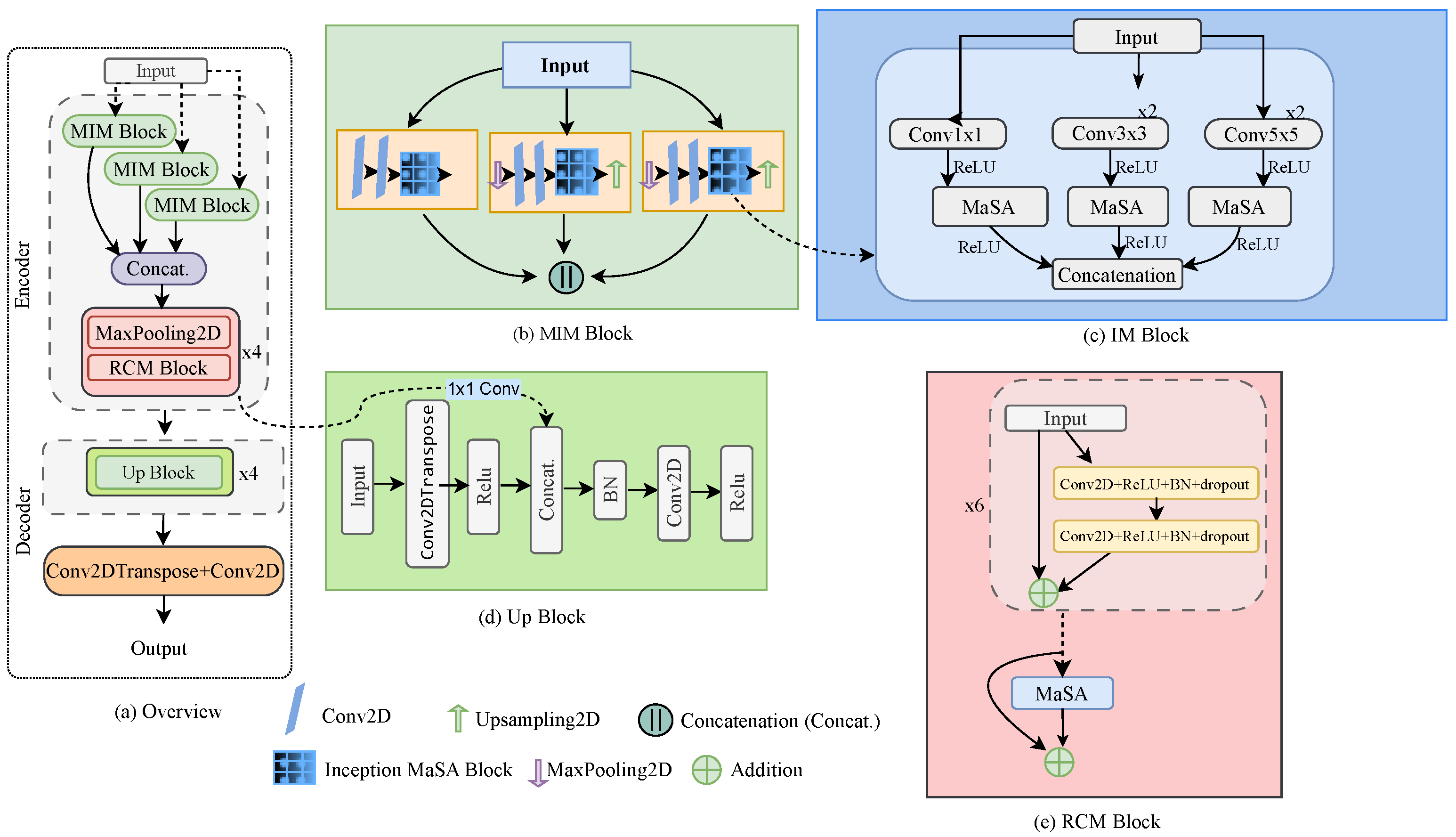
The proposed MIMAR-Net consists of an encoder and decoder, as shown in Figure 1. The encoder processes input images using multiscale MaSA blocks, which combine convolutional layers, MaSA mechanisms, and upsampling to extract features at various scales. Inception MaSA blocks apply self-attention, while the residual convolutional MaSA block enhances features through convolution, self-attention, and residual connections. The decoder reconstructs the output by upsampling feature maps and merging them with skip connections from the encoder. MIMAR-Net is conceptually designed as an encode–decode pipeline specifically for single-image super-resolution. The method begins with a multiscale stem that takes in a single image and extracts complementary features at native, half, and quarter resolution using 1 × 1/3 × 3/5 × 5 convolutions. A lightweight Manhattan Self-Attention (MaSA) module then reweights these features along horizontal and vertical neighborhoods to, on the one hand, accentuate edges and shaped textures while, on the other, reducing noise. The forward pass through the encoder reduces spatial dimensionality while progressively constructing a compact representation, and multiple skip connections preserve fine details at each stage. The learned upsampling performed by the decoder uses transposed convolutions, and at every step of the upsampling process, the decoder fuses the upsampled features with skip connections. A final 1 × 1 projection layer maps the fused representation to the super-resolved image to generate sharper and higher fidelity reconstructions under underwater degradation. The following subsections provide a detailed explanation of each layer in MIMAR-Net, describing the function of each layer and providing detailed mathematical formulations.

3.1. Encoder Part

The input image is initially processed through three multiscale MaSA blocks, each incorporating convolutional layers, Manhattan Self-Attention (Inception MaSA) blocks, and upsampling operations to extract features at different scales. The encoder consists of convolutional layers and a residual convolutional MaSA block, which includes self-attention mechanisms.

3.1.1. Inception MaSA Block

The Manhattan Self-Attention block applies self-attention mechanisms to input features processed through convolutional layers at various scales. Given an input tensor ${\mathrm{X}}_{\mathrm{in}}$ with dimensions $H\times W\times C$, H and W represent the height and width of the input feature map, and C denotes the number of channels.

$\mathbf{1}\times \mathbf{1}$ Convolution and Self-Attention: The input tensor, $X_{\mathrm{in}}$, undergoes a 1 × 1 convolution followed by ReLU activation as

$$X_{1\times 1}=\sigma \left(\mathcal{C}\left(X_{\mathrm{in}},f_{1\times 1},(1,1)\right)\right)$$

(1)

where $\sigma$ denotes the ReLU function, $\mathcal{C}$ represents the Conv2D operation, and $f_{1\times 1}$ is the number of filters. The result is processed through Manhattan Self-Attention in this way

$$A_{1\times 1}=\sigma \left(\mathcal{M}\left(X_{1\times 1}\right)\right)$$

(2)

where $\mathcal{M}$ represents the MaSA (Manhattan Self-Attention) operation.

$\mathbf{3}\times \mathbf{3}$ Convolution and Self-Attention: Similarly, $X_{\mathrm{in}}$ is processed with double $3\times 3$ convolutions as follows:

$$X_{3\times 3}=\sigma \left(\mathcal{C}\left(\mathcal{C}\left(X_{\mathrm{in}},f_{3\times 3},(3,3)\right),f_{3\times 3},(3,3)\right)\right)$$

(3)

then through Manhattan Self-Attention as

$$A_{3\times 3}=\sigma \left(\mathcal{M}\left(X_{3\times 3}\right)\right)$$

(4)

$\mathbf{5}\times \mathbf{5}$ Convolution and Self-Attention: The input is also processed via double $5\times 5$ convolutions like so

$$X_{5\times 5}=\sigma \left(\mathcal{C}\left(\mathcal{C}\left(X_{\mathrm{in}},f_{5\times 5},(5,5)\right),f_{5\times 5},(5,5)\right)\right)$$

(5)

followed by Manhattan Self-Attention as

$$A_{5\times 5}=\sigma \left(\mathcal{M}\left(X_{5\times 5}\right)\right)$$

(6)

Concatenation and Final Convolution: All attention outputs are concatenated as follows

$$A_{\mathrm{concat}}=A_{1\times 1}\parallel A_{3\times 3}\parallel A_{5\times 5}$$

(7)

Here, ‖ represents the Concatenate operation.

3.1.2. Manhattan Self-Attention Mechanism

MaSA extends the traditional self-attention mechanism by incorporating a spatial prior based on the Manhattan distance, evolving from the retention mechanism in RetNet [29]. It employs a BiRetention mechanism as

$$BiRetention\left(\mathbf{X}\right)=(Q{K}^T\circ D^{Bi})V$$

(8)

The interaction between n-th and m-th tokens is represented by the expression $D_{nm}^{Bi}={\gamma }^{|n-m|}$, which highlights the diminishing influence as distance increases. MaSA expands this decay matrix to take Manhattan distances into account for 2D data, like images as

$$D_{nm}^{2D}={\gamma }^{|x_n-x_m|+|y_n-y_m|}$$

(9)

With regard to spatial decay, the fundamental MaSA equation is

$$MaSA\left(\mathbf{X}\right)=(Softmax\left(Q{K}^T\right)\circ D_{2D})V$$

(10)

where the horizontal and vertical directions’ attention scores are independently calculated as

$$MaSA\left(\mathbf{X}\right)=Att{n}_H{\left(Att{n}_V\right)}^T$$

(11)

with ${\mathrm{Attn}}_H=\mathrm{Softmax}\left(Q_H{K}_H^{\top }\right)\odot D_H \mathrm{and} {\mathrm{Attn}}_W=\mathrm{Softmax}\left(Q_W{K}_W^{\top }\right)\odot D_W.$

To further enhance local expression capabilities, MaSA also employs the Local Context Enhancement (LCE) module inspired by [30]. The model then becomes as follows

$${\mathbf{X}}_{out}=MaSA\left(\mathbf{X}\right)+LCE\left(V\right)$$

(12)

In this case, MaSA’s capacity to use spatial relationships for improved attention modeling in vision tasks is strengthened by LCE’s use of depthwise convolutions.

3.1.3. Residual Convolutional MaSA Block

The Residual Convolutional Attention Block is another component of our model, designed to enhance feature representations through iterative convolutional operations and self-attention mechanisms.

Cascaded Residual Convolution Block: Given an input tensor $\mathbf{X}\in {\mathbb{R}}^{H\times W\times C}$, the residual convolutional MaSA block begins by applying a series of convolutional operations combined with batch normalization, ReLU activation, and dropout for regularization, written as

$${\mathbf{X}}_{\mathrm{conv}}^{\left(1\right)}=\delta \left(\mathcal{D}\left(\beta \left(\mathcal{C}\left(\mathbf{X},\mathcal{F},(\mathcal{K},\mathcal{K})\right)\right)\right)\right)$$

(13)

where $\mathcal{C}$ denotes the Conv2D operation with filters $\mathcal{F}$ and kernel size $\mathcal{K}$. $\beta$ is the batch normalization function. $\delta$ is the ReLU activation function. $\mathcal{D}$ is the dropout operation with rate $\mathcal{P}$.

This operation is then repeated once again as follows

$${\mathbf{X}}_{\mathrm{conv}}^{\left(2\right)}=\delta \left(\mathcal{D}\left(\beta \left(\mathcal{C}\left({\mathbf{X}}_{\mathrm{conv}}^{\left(1\right)},\mathcal{F},(\mathcal{K},\mathcal{K})\right)\right)\right)\right)$$

(14)

Accordingly, this convolution is iteratively performed with a residual connection, allowing the feature maps to evolve over multiple steps, expressed as

$${\mathbf{X}}_{res}^{\left(i\right)}={\mathbf{X}}_{\mathrm{conv}}^{\left(2\right)(i-1)}+\mathbf{X}, \mathrm{for}i=1,2,\dots ,T$$

(15)

Here, T is set to be 6 in this work.

Integration of Manhattan Self-Attention (MaSA): Following a sequence of residual convolutional operations, the feature map is passed through the MaSA module, which attends to spatially relevant features. The output after integrating MaSA is expressed as

$$\tilde{\mathbf{Y}}={\mathbf{X}}_{\mathrm{conv}}^{\left(2\right)\left(T\right)}+\mathrm{MaSA}\left({\mathbf{X}}_{\mathrm{conv}}^{\left(2\right)\left(T\right)}\right)$$

(16)

3.2. Decoder Part

The decoder reconstructs the high-resolution image using deep features generated by the encoder [31]. It consists of multiple upsampling blocks that utilize Conv2DTranspose layers to upscale feature maps and merge them with corresponding skip connections from the encoder, recovering spatial details.

Up Block: The Up block is a key component in the decoder, responsible for upsampling the feature map and merging it with a skip connection from the encoder.

Transposed Convolution for Upsampling: Given an input tensor $X_{\mathrm{in}}$, the first step in the upsampling block is to increase the spatial resolution of the feature map using a transposed convolution, formulated as

$$X_{\mathrm{up}}=\sigma \left(g(X_{\mathrm{in}},f,(k,k))\right),$$

(17)

where $g(·)$ represents the transposed convolution operation with a kernel size of $(k,k)$ and f output filters, and $\sigma (·)$ denotes a non-linear activation function.

Processing the Skip Connection: $\xi$ denotes as the skip connection from the corresponding encoder and is processed via a $1\times 1$ convolution as follows

$$S_{\mathrm{conv}}=C(\xi ,f,(1,1))$$

(18)

If the spatial dimensions of the skip connection $\xi$ do not match the upsampled feature map $S_{up}$, it is resized using nearest-neighbor interpolation with a scale factor.

Concatenation: The upsampled feature map $X_{up}$ and the processed skip connection $S_{up}$ are concatenated along the channel dimension as

$$X_{\mathrm{concat}}=X_{\mathrm{up}}\parallel S_{\mathrm{up}}$$

(19)

Batch Normalization and Convolution: The concatenated feature map is passed through a batch normalization layer, followed by a standard convolution as follows

$$X_{\mathrm{norm}}=\beta \left(X_{\mathrm{concat}}\right)$$

(20)

$$X_{\mathrm{conv}}=\sigma (\mathcal{C}(X_{\mathrm{norm}},f,(k,k))$$

(21)

3.3. Loss Function

We use a compound loss function that integrates three metrics, including the structural similarity index (SSIM) [32], mean squared error (MSE) [33], and mean absolute error (MAE) [33], to optimize our model for underwater image SR.

SSIM Loss: The structural similarity index (SSIM) loss, denoted as ${\mathcal{L}}_{SSIM}$, measures the similarity between the feature representation of the enhanced image and the reference image. The SSIM between two images $k_i$ and $k_i^{\ast }$ is computed as

$$\mathrm{SSIM}(k_i,k_i^{\ast })={\displaystyle \frac{(2{\mu }_x{\mu }_y+C_1)(2{\sigma }_{xy}+C_2)}{({\mu }_x^2+{\mu }_y^2+C_1)({\sigma }_x^2+{\sigma }_y^2+C_2)}}$$

(22)

where ${\mu }_x$ and ${\mu }_y$ represent the means, ${\sigma }_x^2$ and ${\sigma }_y^2$ denote the variances, and ${\sigma }_{x}y$ is the covariance of the images. The SSIM loss is then defined as

$${\mathcal{L}}_{SSIM}=1-\mathrm{SSIM}(k_i,k_i^{\ast })$$

(23)

MSE Loss: Mean squared error (MSE) assesses the degree of variability in the data. The MSE loss is calculated by taking the sum of the squared differences between the enhanced image k and the reference image $k^{\ast }$ across all pixels as

$${\mathcal{L}}_{MSE}={\displaystyle \frac{1}{N}}\sum _{i=1}^N{(k_i-k_i^{\ast })}^2$$

(24)

MAE Loss: The mean absolute error (MAE) loss, denoted as ${\mathcal{L}}_{MAE}$, measures the average absolute difference between predicted and actual pixel values. The MAE loss is calculated as

$${\mathcal{L}}_{MAE}={\displaystyle \frac{1}{N}}\sum _{i=1}^N|k_i-k_i^{\ast }|$$

(25)

where N is the total number of pixels. $k_i$ represents the pixel value of the enhanced image. $k_i^{\ast }$ represents the corresponding pixel value in the reference image.

Accordingly, the total loss function defined in our method can be written as

$${\mathcal{L}}_{total}={\lambda }_0{\mathcal{L}}_{SSIM}+{\lambda }_1{\mathcal{L}}_{MSE}+{\lambda }_2{\mathcal{L}}_{MAE}$$

(26)

The weights ${\lambda }_0$, ${\lambda }_1$, and ${\lambda }_2$ of the total loss function are empirically chosen to be 0.6, 0.2, and 0.2, respectively, based on an ablation study. The configuration of the loss is created to prioritize structural similarity (SSIM) with adequate attention paid to pixel-level accuracy (MSE) and robustness to outliers (MAE), which are complementary aspects crucial for underwater image SR. As specified in Section 4.6 we assess model performance for five different weight combinations. The configuration $({\lambda }_0=0.6,{\lambda }_1=0.2,{\lambda }_2=0.2)$ yields the best PSNR, SSIM, and UIQM values among the combinations tried, justifying its selection. This empirical tuning gives a balanced and efficient optimization process that enhances both perceptual and quantitative image quality metrics.

4. Experiments

4.1. Dataset

The proposed model’s performance is evaluated on three publicly available underwater image datasets: UFO-120 [17], USR-248 [16], and EUVP [12]. The UFO-120 dataset, used for Simultaneous Enhancement and Super-Resolution (SESR) tasks, contains 120 synthetic test images and 1500 synthetic training images. In contrast, the USR-248 dataset, designed for Single-Image Super-Resolution (SISR) tasks, provides 560 low-resolution image sets at various scales (80 × 60, 160 × 120, and 320 × 240) and includes 1060 paired images for training along with 248 reference images for comprehensive model assessment. The EUVP training dataset consists of 11,435 paired underwater images and the test set comprises 515 image pairs. In our experiment, all images from these three datasets are resized to 128 × 128 to match the input requirements of the proposed model.

4.2. Training Details

For training MIMAR-Net, we use an NVIDIA RTX 6000 Ada Generation GPU. The model uses Stochastic Gradient Descent (SGD) as the optimizer, with a learning rate of 0.001, momentum of 0.9, Nesterov acceleration, and gradient clipping (clip value = 1.0), with a decay rate of $1\times {10}^{-6}$ to ensure stable convergence. To achieve reproducibility, we apply the same random seed value in all our experiments. All input images are normalized to the range of [0, 1]. During training, low-resolution inputs are created by downsampling the original high-resolution RGB images using area-based interpolation, while the original images are also used as corresponding high-resolution targets. The dataset split is predetermined as the UFO-120 and USR-248, and the EUVP datasets already have the training and testing images separated. The model has 22,793,729 parameters in total and 22,779,137 trainable and 14,592 non-trainable parameters among them. The training is carried out for 120 epochs at a batch size of 8, which is determined to utilize all of the GPUs. A batch size of 8 is selected to maximize GPU memory usage while ensuring stable training dynamics. The initial learning rate of 0.001 is chosen because it is a commonly used starting point for super-resolution tasks and also provides a good balance between convergence speed and stability [34,35,36]. We use SGD with Nesterov momentum as a standard optimizer for image restoration tasks [35,37,38]. This setting is used to find a stable, high-performing solution in a good balance of convergence speed and generalization.

4.3. Quantitative Comparisons

This section presents a quantitative analysis of our proposed MIMAR-Net model against state-of-the-art SR methods on the UFO-120, USR-248, and EUVP datasets. We evaluate the models at $\times 2$ and $\times 4$ upscaling rates using common full-reference and no-reference metrics, including PSNR [39], SSIM [32], UIQM [40], Learned Perceptual Image Patch Similarity (LPIPS) [41], and Fréchet Inception Distance (FID) [42]. The PSNR and SSIM measure how close the generated image is to the ground truth, while the UIQM gives an indication of the color, contrast, and sharpness of the generated images. LPIPS assesses perceptual similarity between a pair of images using deep features from neural networks, which correlates better with human judgment in perception than previous pixel-wise metrics. FID calculates the quality and diversity of generated images by measuring the statistics (i.e., mean and covariance) of neural features from both real images and generated images, all measured using the Inception network. The upscaled images by the models are compared with ground truth high-resolution images for full-reference evaluation with the PSNR and SSIM and directly used for no-reference evaluation with the UIQM.

UFO-120: To evaluate the statistical strength of our findings, we assess all the models on UFO-120 test images and report mean and standard deviation (SD) for PSNR, SSIM, UIQM, LPIPS, and FID at both $\times 2$ and $\times 4$ upscaling. As shown in

Table 1. Quantitative evaluation of SISR models on the UFO-120 dataset at $\times 2$ upscaling. We report mean ± SD for PSNR, SSIM, UIQM, LPIPS, and FID. Best results are in bold. The ↑ indicates that higher values represent better performance and the ↓ indicates that lower values represent better performance.

Model	PSNR (dB) ↑	SSIM ↑	UIQM ↑	LPIPS ↓	FID ↓
SRDRM [16]	26.46 ± 1.89	0.8412 ± 0.06	2.5811 ± 0.012	0.0018	2.66
SRDRM-GAN [16]	27.93 ± 2.10	0.8710 ± 0.05	2.5981 ± 0.011	0.0016	2.62
SRCNN [14]	28.25 ± 3.18	0.8780 ± 0.05	2.5982 ± 0.010	0.0017	2.51
FSRCNN [15]	28.01 ± 3.17	0.8720 ± 0.05	2.6002 ± 0.010	0.0022	2.76
ESPCN [23]	29.02 ± 3.23	0.8419 ± 0.05	2.6018 ± 0.011	0.0025	2.80
EDSR [24]	29.00 ± 3.10	0.8710 ± 0.05	2.5701 ± 0.010	0.0015	2.46
Deep SESR [17]	28.58 ± 2.21	0.8603 ± 0.05	2.5907 ± 0.010	0.0018	2.72
Deep WaveNet [25]	26.91 ± 2.72	0.8359 ± 0.12	2.5910 ± 0.009	0.0022	2.67
MIMAR-Net (Ours)	29.18 ± 3.40	0.8831 ± 0.05	2.6788 ± 0.008	0.0012	2.49

, MIMAR-Net obtains the highest mean PSNR (29.18 dB), SSIM (0.8831), and UIQM (2.6788) at $\times 2$ upscaling, indicating improved fidelity for image reconstruction and structural similarity. MIMAR-Net also retains the top score at $\times 4$ upscaling for PSNR, SSIM, UIQM, and LPIPS, as shown in

Table 2. Quantitative evaluation of SISR models on the UFO-120 dataset at $\times 4$ upscaling. We report mean ± SD for PSNR, SSIM, UIQM, LPIPS, and FID. Best results are in bold. The ↑ indicates that higher values represent better performance and the ↓ indicates that lower values represent better performance.

Model	PSNR (dB) ↑	SSIM ↑	UIQM ↑	LPIPS ↓	FID ↓
SRDRM [16]	25.77 ± 2.71	0.7345 ± 0.10	2.5805 ± 0.010	0.0024	2.72
SRDRM-GAN [16]	25.94 ± 2.75	0.7353 ± 0.09	2.5859 ± 0.009	0.0020	2.67
SRCNN [14]	26.34 ± 3.39	0.7432 ± 0.11	2.5836 ± 0.007	0.0021	2.57
FSRCNN [15]	26.54 ± 3.04	0.7472 ± 0.10	2.5844 ± 0.008	0.0026	2.80
ESPCN [23]	26.54 ± 3.20	0.7485 ± 0.10	2.5852 ± 0.008	0.0031	2.83
EDSR [24]	26.59 ± 3.27	0.7490 ± 0.10	2.5648 ± 0.008	0.0019	2.51
Deep SESR [17]	25.89 ± 2.71	0.7318 ± 0.10	2.5859 ± 0.010	0.0025	2.78
Deep WaveNet [25]	25.97 ± 2.71	0.7381 ± 0.12	2.5842 ± 0.008	0.0028	2.75
MIMAR-Net (Ours)	26.79 ± 3.16	0.7517 ± 0.10	2.6528 ± 0.008	0.0018	2.55

, outperforming all of the models in this challenging scenario. Other methods, such as SRCNN, FSRCNN, and ESPCN, perform fairly but ultimately underperform MIMAR-Net. GAN-based models (SRDRM-GAN) and wavelet-inspired models (Deep WaveNet) have lower performances in terms of PSNR, SSIM, and UIQM. Moreover, for LPIPS and FID metrics, MIMAR-Net achieves the lowest LPIPS (0.0012 at $\times 2$ and 0.0018 at $\times 4$) and has competitive FID values (2.49 at $\times 2$, 2.55 at $\times 4$) only behind EDSR. This result demonstrates that MIMAR-Net can reconstruct high-fidelity images while also creating visually appealing and perceivably correct images.

USR-248: To evaluate consistency and robustness of performance across samples, we evaluate all models on the USR-248 test set, and report mean and standard deviation (SD) of PSNR, SSIM, UIQM, LPIPS, and FID for both $\times 2$ and $\times 4$ upscaling. The results in

Table 3. Quantitative evaluation of SISR models on the USR-248 dataset at $\times 2$ upscaling. We report mean ± SD for PSNR, SSIM, UIQM, LPIPS, and FID. Best results are in bold. The ↑ indicates that higher values represent better performance and the ↓ indicates that lower values represent better performance.

Model	PSNR (dB) ↑	SSIM ↑	UIQM ↑	LPIPS ↓	FID ↓
SRDRM [16]	26.74 ± 1.91	0.8551 ± 0.05	2.9280 ± 0.009	0.0021	2.63
SRDRM-GAN [16]	27.91 ± 2.05	0.8678 ± 0.05	2.9087 ± 0.008	0.0019	2.57
SRCNN [14]	28.05 ± 3.39	0.8764 ± 0.05	2.8289 ± 0.010	0.0018	2.48
FSRCNN [15]	27.63 ± 3.01	0.8696 ± 0.05	2.8009 ± 0.010	0.0021	2.75
ESPCN [23]	28.08 ± 3.18	0.8615 ± 0.06	2.8011 ± 0.009	0.0024	2.77
EDSR [24]	29.01 ± 3.26	0.8612 ± 0.05	2.8020 ± 0.010	0.0017	2.49
Deep SESR [17]	27.61 ± 2.15	0.8703 ± 0.05	2.7216 ± 0.011	0.0020	2.66
Deep WaveNet [25]	25.98 ± 2.68	0.8244 ± 0.13	2.7091 ± 0.010	0.0023	2.71
MIMAR-Net (Ours)	29.10 ± 2.87	0.8827 ± 0.06	2.9035 ± 0.007	0.0013	2.44

indicate that MIMAR-Net consistently outperforms all competing models in PSNR and SSIM at both scales. At $\times 2$, MIMAR-Net is reported to achieve a PSNR of 29.10 dB and 0.8827 for SSIM, signifying both fidelity and structural similarity. MIMAR-Net is also shown to obtain UIQM of 2.9035, positioning it in the top three for underwater perceptual quality. At $\times 4$ showing in

Table 4. Quantitative evaluation of SISR models on the USR-248 dataset at $\times 4$ upscaling. We report mean ± SD for PSNR, SSIM, UIQM, LPIPS, and FID. Best results are in bold. The ↑ indicates that higher values represent better performance and the ↓ indicates that lower values represent better performance.

Model	PSNR (dB) ↑	SSIM ↑	UIQM ↑	LPIPS ↓	FID ↓
SRDRM [16]	22.67 ± 2.67	0.7108 ± 0.08	2.9029 ± 0.010	0.0024	2.70
SRDRM-GAN [16]	25.41 ± 2.71	0.7044 ± 0.09	2.8871 ± 0.007	0.0021	2.65
SRCNN [14]	26.27 ± 3.29	0.7411 ± 0.10	2.8039 ± 0.009	0.0020	2.56
FSRCNN [15]	25.72 ± 3.07	0.7387 ± 0.09	2.7847 ± 0.009	0.0024	2.79
ESPCN [23]	26.28 ± 3.12	0.7454 ± 0.10	2.7959 ± 0.008	0.0028	2.81
EDSR [24]	26.33 ± 3.21	0.7421 ± 0.10	2.7851 ± 0.009	0.0017	2.50
Deep SESR [17]	24.62 ± 2.88	0.7391 ± 0.11	2.6755 ± 0.010	0.0023	2.74
Deep WaveNet [25]	23.83 ± 2.84	0.6849 ± 0.12	2.6860 ± 0.009	0.0025	2.72
MIMAR-Net (Ours)	26.65 ± 3.11	0.7496 ± 0.09	2.8889 ± 0.008	0.0015	2.52

, MIMAR-Net still shows competitive performance, achieving 26.65 dB for PSNR, 0.7496 ± 0.09 SSIM, and the second-best UIQM of 2.8889. Although SRDRM is able to achieve slightly better UIQM, it performs significantly worse for PSNR and SSIM. Deep WaveNet performs consistently the lowest across all metrics. MIMAR-Net achieves LPIPS of 0.0015, which is the best score, alongside an FID of 2.52, which yields the second best (after EDSR at 2.50). These results provide further evidence of MIMAR-Net’s robustness and generalization capabilities in maintaining high-quality reconstruction performance across multiple metrics.

EUVP: We assess the performance of the models on the EUVP dataset and report mean and standard deviation (SD) for PSNR, SSIM, UIQM, LPIPS, and FID metrics for both $\times 2$ and $\times 4$ configurations. As seen in

Table 5. Quantitative evaluation of SISR models on the EUVP dataset at $\times 2$ upscaling. We report mean ± SD for PSNR, SSIM, UIQM, LPIPS, and FID. Best results are in bold. The ↑ indicates that higher values represent better performance and the ↓ indicates that lower values represent better performance.

Model	PSNR (dB) ↑	SSIM ↑	UIQM ↑	LPIPS ↓	FID ↓
SRDRM	30.42 ± 1.98	0.9033 ± 0.03	4.0480 ± 0.012	0.0019	2.41
SRDRM-GAN	37.17 ± 2.25	0.9707 ± 0.02	4.1671 ± 0.010	0.0014	2.37
SRCNN	37.42 ± 2.38	0.9701 ± 0.02	4.1208 ± 0.011	0.0013	2.28
FSRCNN	36.92 ± 2.52	0.9658 ± 0.02	4.1049 ± 0.010	0.0016	2.32
ESPCN	36.90 ± 2.40	0.9662 ± 0.02	4.1110 ± 0.009	0.0018	2.25
EDSR	37.68 ± 2.30	0.9660 ± 0.02	4.1185 ± 0.009	0.0012	2.22
Deep SESR	30.60 ± 1.85	0.9383 ± 0.03	4.2405 ± 0.009	0.0017	2.48
Deep WaveNet	31.16 ± 2.00	0.9063 ± 0.04	4.0106 ± 0.010	0.0020	2.51
MIMAR-Net (Ours)	38.96 ± 2.43	0.9720 ± 0.02	4.1989 ± 0.010	0.0011	2.18

, MIMAR-Net exhibits the highest overall performance on PSNR, SSIM, LPIPS, and FID metrics. For $\times 2$ upsampling, MIMAR-Net produces the highest PSNR of 38.96 dB and SSIM of 0.9720. Although Deep SESR performs slightly better with UIQM (4.2405), MIMAR-Net experiences second-best perceptual quality with UIQM (4.1989). For $\times 4$ upsampling, shown in

Table 6. Quantitative evaluation of SISR models on the EUVP dataset at $\times 4$ upscaling. We report mean ± SD for PSNR, SSIM, UIQM, LPIPS, and FID. Best results are in bold. The ↑ indicates that higher values represent better performance and the ↓ indicates that lower values represent better performance.

Model	PSNR (dB) ↑	SSIM ↑	UIQM ↑	LPIPS ↓	FID ↓
SRDRM	29.93 ± 2.04	0.8949 ± 0.03	3.5821 ± 0.010	0.0021	2.49
SRDRM-GAN	37.32 ± 2.40	0.9505 ± 0.02	3.6878 ± 0.011	0.0016	2.41
SRCNN	37.13 ± 2.36	0.9499 ± 0.02	3.5231 ± 0.009	0.0015	2.31
FSRCNN	36.01 ± 2.48	0.9498 ± 0.02	3.6045 ± 0.010	0.0019	2.30
ESPCN	36.11 ± 2.47	0.9402 ± 0.02	3.6104 ± 0.010	0.0022	2.35
EDSR	37.43 ± 2.51	0.9516 ± 0.02	3.6060 ± 0.009	0.0014	2.26
Deep SESR	30.21 ± 1.96	0.9281 ± 0.03	3.5181 ± 0.008	0.0020	2.54
Deep WaveNet	31.09 ± 2.10	0.8951 ± 0.03	3.7936 ± 0.008	0.0021	2.59
MIMAR-Net (Ours)	38.39 ± 2.61	0.9549 ± 0.02	3.6278 ± 0.009	0.0013	2.22

, MIMAR-Net maintains solid performance with PSNR of 38.39 dB and SSIM of 0.9549, indicating more robustness under a higher upsampling scale. While Deep Wavenet records the best UIQM for $\times 4$, it lags in PSNR and SSIM metrics. Regarding perceptual similarity, MIMAR-Net achieves the lowest LPIPS values (0.0011 at $\times 2$ and 0.0013 at $\times 4$), signifying good visual similarity to the ground truth. Moreover, it also outperforms all other models in FID (2.18 at $\times 2$ and 2.22 at $\times 4$), which indicates its strong ability to produce realism and high-quality reconstructions.

4.4. Generalization to Non-Underwater Dataset

To evaluate the generalization ability of MIMAR-Net outside of underwater images, we further use it on natural images in the BSD100 dataset. As presented in

Table 7. Quantitative evaluation of SISR models on the BSD100 dataset at $\times 4$ upscaling, using PSNR and SSIM. Best results are in bold. The ↑ indicates that higher values represent better performance.

Model	Year	PSNR (dB) ↑	SSIM ↑
SRGAN [43]	2017	25.17	0.6408
SRResNet [43]	2017	26.32	0.6940
MS-LapSRN [44]	2017	27.41	0.7306
HGFormer [45]	2025	27.88	0.7480
EARFA [46]	2024	27.75	0.7431
MIMAR-Net (Ours)	N/A	26.16	0.7395

, MIMAR-Net exhibits an SSIM (0.7395) that is approximately on par with higher than those of the Super-Resolution Generative Adversarial Network (SRGAN) [43] (0.6408), and Super-Resolution Residual Network (SRResNet) [43] (0.6940) MIMAR-Net also achieves a PSNR of 26.16 dB, which is slightly lower than a few other methods, but has an SSIM exhibiting much greater performance at the detail-level structural preservation. Consistent with its SSIM performance, MIMAR-Net notably achieves greater PSNR than SRGAN. In terms of SSIM, MIMAR-Net achieves a higher SSIM than SRGAN, SRResNet, MS-LapSRN [44], despite being trained exclusively on underwater datasets. Collectively, these analyses provide evidence that MIMAR-Net has governed stronger generalizability to the domain of natural images and demonstrates that it does not succumb to overfitting of highly domain-specific training data. We also compare with the MS-LapSRN method, which focuses on detail recovery through progressive refinement, similar to MIMAR-Net’s purpose of textural and structural edges recovery with details. Hourglass Transformer (HGFormar) [45] uses the hourglass attention structure and Entropy Attention and Receptive Field Augmentation network (EARFA) [46] applied attention mechanism. The adoption of allocating multiscale features and progressive upsampling can render them structurally similar, as well as being relevant incumbent baseline methods across domains to evaluate generalizability.

4.5. Qualitative Comparisons

The qualitative evaluation provides visual comparisons of how well each model handles the complexities of the underwater environment, such as the preservation of fine details, the accuracy of color reproduction, and the enhancement of contrast and sharpness.

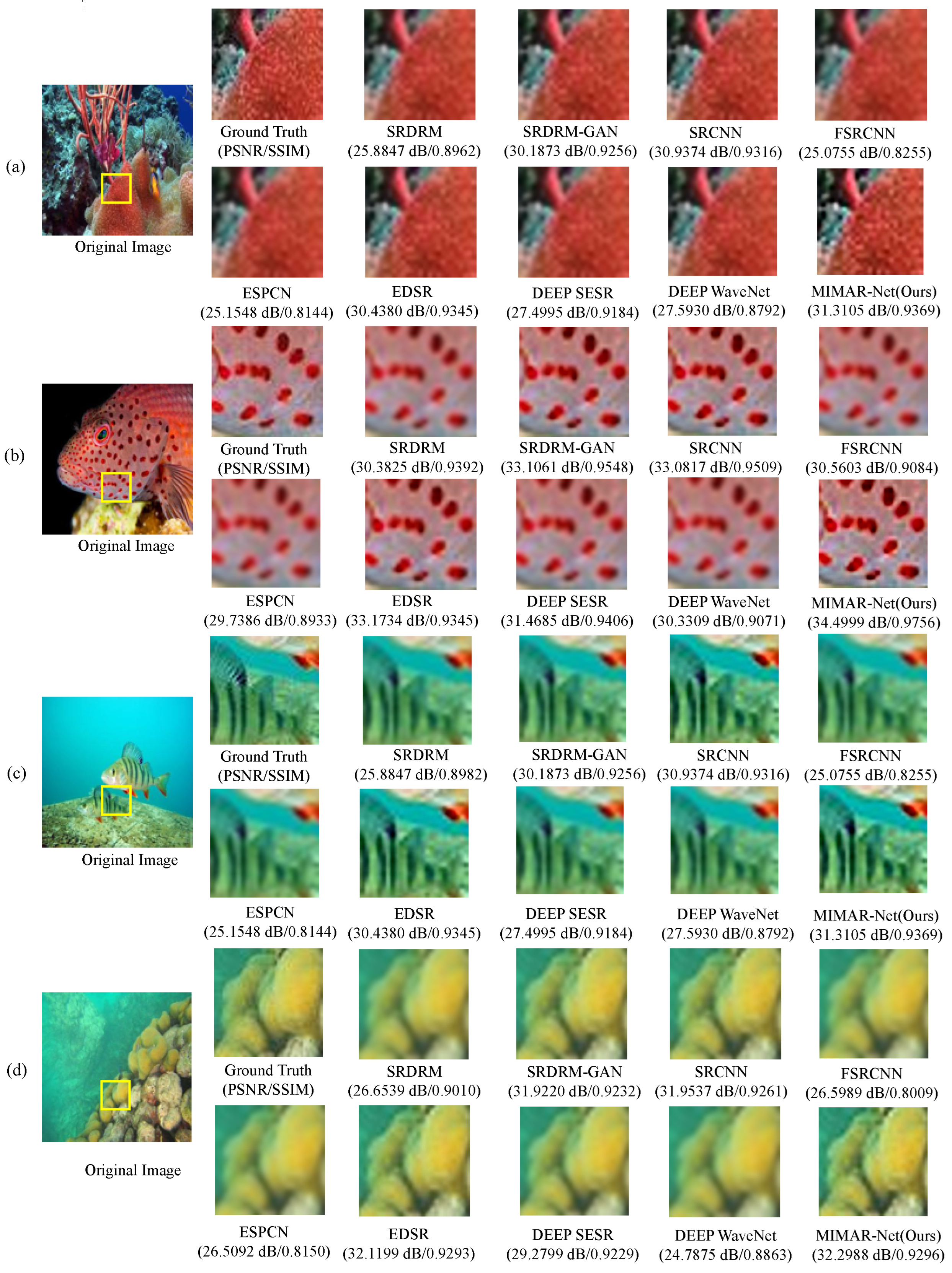
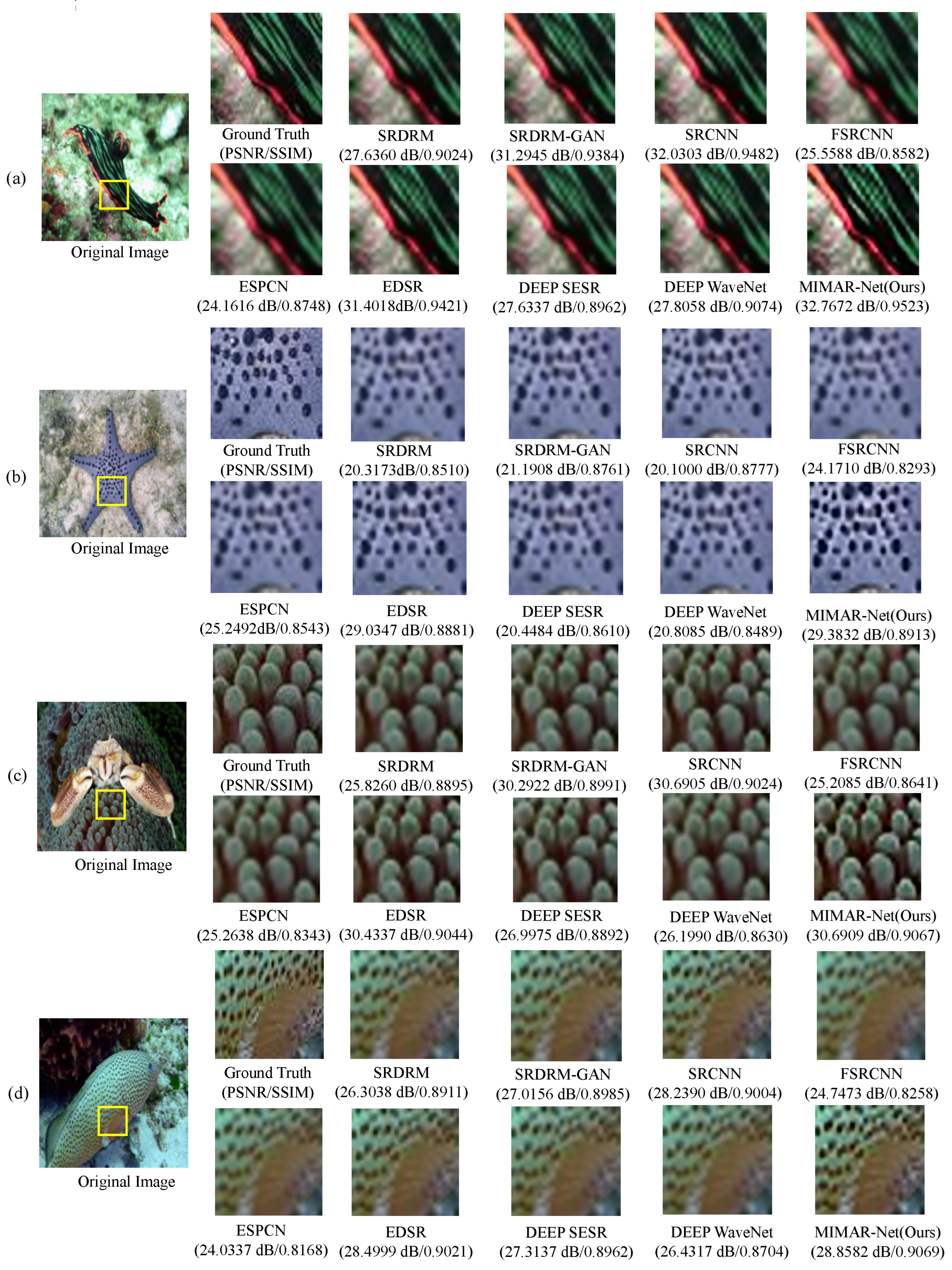
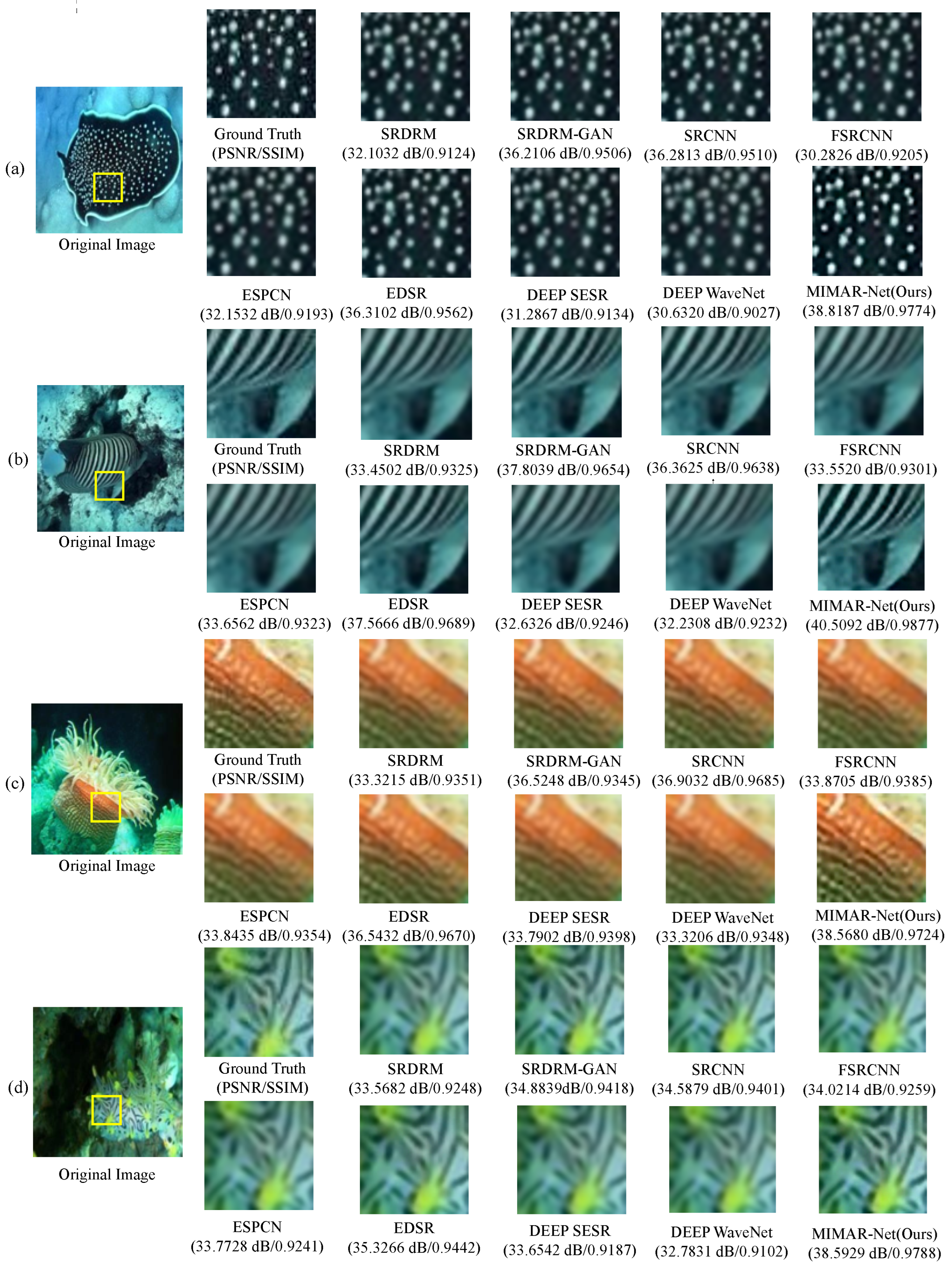
In this section, we present a qualitative comparison of our proposed model against several state-of-the-art SR models, including EDSR [24], SRCNN [14], FSRCNN [15], ESPCN [23], SRDRM [16], SRDRM-GAN [16], Deep WaveNet [25], and Deep SESR [17]. The comparisons are performed on three different datasets: UFO-120, USR-248, and EUVP. We run the selected models on the $\times 2$ downsampled original images from three selected datasets. Then, we visually inspect the output performance of the models for random images to check if they can improve the original images and restore the ground truth resolution and details, as shown in Figure 2, Figure 3 and Figure 4. Similar trends can be observed across these datasets, with a clear improvement to the original images by most models. The SRDRM, FSRCNN, ESPCN, DEEP SESR, and DEEP WaveNet lost more details in the upscaling reconstruction process compared to other models, including ours, for all three datasets. The SRDRM-GAN did comparatively lower performance on the UFO-120 and USR-248 datasets but performed well on the EUVP dataset. For images containing complex structures and details, FSRCNN and ESPCN are behind all other models, while our model successfully preserves most of the details and provides good color accuracy in complex scenes. Upgraded models, such as the SRDRM-GAN, perform better than the stock SRDRM. But the SRCNN performs better than the FSRCNN in terms of underwater conditions. The EDSR model achieves better performance than other models, but it cannot outperform our model. Our MIMAR-Net model outperforms all other models in terms of detail preservation and color correctness.

UFO-120: We evaluate models at $\times 2$ and $\times 4$ upsampling factors to assess their ability to enhance resolution and maintain image quality. Figure 2 provides visual comparisons of $\times 2$ upsampling outputs. From the visual comparisons, it is evident that our MIMAR-Net model consistently produces better results in various underwater settings, thus outperforming existing methods. In the first example shown in Figure 2a, our method can retain fine coral structures and improve the color gamut for reds and blues, which are often blurred or oversmoothed by other methods, such as SRDRM, DEEP SESR, and DEEP WaveNet. FSRCNN and ESPCN present texture artifacts and loss of fine details. For the second one, Figure 2b, the red spots on the fish contrast sharply against the background when enhanced by our method. Competing methods tend to lose edge sharpness or blur the red pattern. EDSR, SRDRM-GAN, and SRCNN perform effectively but are still not perfect in retaining the fine dot-like structures and the overall clarity. The third example, Figure 2c, includes vertical striped fish patterns, and it looks like our method has also done well in keeping stripes intact with sharp edges and color transitions. In the final example, Figure 2d, our proposed model recovers fine surface variations and realistic shading, providing a natural and sharp appearance. On the other hand, we see it somewhat blurred with other models.

USR-248: For the USR-248 dataset, we qualitatively compare our proposed model with leading SR methods at $\times 2$ and $\times 4$ upsampling factors. As shown in Figure 3, our model consistently outperforms others at $\times 2$ upsampling by maintaining fine details, enhancing contrast, and accurately restoring colors. In the first example, Figure 3a, the red and green striped structures are well-resolved and look natural in our result. SRCNN and EDSR also perform well but show slight blurring or loss of line clarity. However, FSRCNN and ESPCN smooth out the stripes together with color distortion, making those fine stripes rather less distinct. In the second example shown in Figure 3b (starfish), the dotted texture on the starfish surface is preserved well by our model, whereas other methods like SRDRM, DEEP SESR, and DEEP WaveNet tend to apply some blur on these dots and FSRCNN introduces even more texture artifacts. EDSR performs quite well but lacks the capacity to separate and define edges. In the third example, Figure 3c, MIMAR-Net effectively preserves the repeated ridge patterns with clear separations and smooth transitions. Other methods introduce visible smoothing (e.g., FSRCNN and ESPCN) or lose subtle surface variations (e.g., DEEP SESR and DEEP WaveNet). In the last example, Figure 3d, our model does an excellent job of recovering the fine-scale patterns and natural transitions between scales. In contrast, techniques like DEEP WaveNet and DEEP SESR typically result in textures that appear somewhat blocky or blurry, while FSRCNN and ESPCN lose a lot of fine detail and create obvious artifacts. Our model produces images with substantially greater visual quality and stronger structural integrity than the state-of-the-art baselines.

EUVP: Figure 4 shows a visual comparison of different models on the EUVP dataset. In the first row, Figure 4a, the model recovers the fine white dot pattern with much better clarity and contrast than SRDRM, FSRCNN, ESPCN, or FSRCNN, all of which have a tendency to blur or oversmooth their outputs slightly. EDSR, SRDRM-GAN, and SRCNN produce somewhat appropriate forms but lack the vibrancy and accuracy in color tones that our model achieves. Striped fish patterns, Figure 4b, with sharp boundaries and bright colors are kept in our results, while the rest of the models blur such stripes or bring in light color distortions. In the third and fourth examples, Figure 4c,d, the textural complexity of corals and marine plants is adequately preserved by our model. The other models seem to blur with color fading, whereas our method sees improvement in contrast, realistic color schemes, and well-defined edges.

4.6. Computational Complexity Analysis

To achieve effective performance in SR, deep neural networks are expected to be computationally efficient for real-time applications, particularly in underwater environments. Most underwater technologies, including AUVs, ROVs, and any portable diving gear, rely on edge devices with an extremely limited processing capacity, memory space, and a lack of power supply. Considering these practical issues, we take a more detailed look at how MIMAR-Net stands with respect to computational efficiency against some commonly known SR models. To evaluate the computational performance of our proposed MIMAR-Net architecture relative to other SR models, parameter and GFLOPs counts per inference on a standard input of 128 × 128 pixels are analyzed. It is seen in

Table 8. GFLOPs and parameter counts for each model (evaluated on 128 × 128 inputs). All models were tested on an NVIDIA RTX 6000 GPU.

Model	Params (M)	GFLOPs
SRDRM	1.78	58.226
SRDRM-GAN	6.99	217.871
SRCNN	0.057	1.894
FSRCNN	0.012	0.404
ESPCN	0.020	0.701
EDSR	43.00	1419.852
Deep SESR	2.07	127.028
Deep WaveNet	10.22	351.149
Lightweight MIMAR-Net (Ours)	9.72	106.89
MIMAR-Net (Ours)	22.78	368.744

that by design, lightweight models such as FSRCNN and ESPCN offer both very low GFLOPs (0.404 G and 0.701 G, respectively) and parameter counts (0.012 M and 0.020 M) and are thus desirable for real-time or resource-constrained applications. However, the lower model complexity limits their ability to recover fine details in difficult situations such as underwater images. In contrast to this, the computational costs of SRDRM-GAN, EDSR, Deep SESR, and Deep WaveNet models are extremely expensive: around 217.871 GFLOPs and 6.99 M parameters for SRDRM-GAN, 1419.852 GFLOPs, and 43 M parameters for EDSR, 127.028 GFLOPs, and 2.07 M parameters for Deep SESR, and 351.149 GFLOPs and 10.22 M parameters for Deep WaveNet.

To achieve a fair trade-off between parameter count and model efficiency, we propose a pruned version of MIMAR-Net, which is named as Lightweight MIMAR-Net, consisting of only a multiscale block and IM block. The findings in Table 8 show that our proposed Lightweight MIMAR-Net achieves a satisfactory trade-off between model complexity and performance. The lightweight model has 9.72 M parameters, requiring 106.89 GFLOPs compared with 22.78 M parameters and 368.74 GFLOPs of the full MIMAR-Net model. This represents a reduction of almost 57% in parameters and 71% in GFLOPs, resulting in an improved computational efficiency. The lightweight version is a good compromise between accuracy (showing in Section 5.3 and efficiency. In addition, the lightweight version offers a complexity-matched baseline, which facilitates a fairer comparison among the models and can be significant for future real-time applications.

5. Ablation Study

In this section, we conduct two ablation studies on the three selected datasets, such as UFO-120, USR-248, and EUVP. In particular, one ablation study focuses on the individual impact of the three terms of the loss function, namely the SSIM, MSE, and MAE losses, and we also studied the impact of the different weights of loss functions, while the other ablation study focuses on the impact of different components of the proposed model on the overall performance.

5.1. Ablation Study on Loss Functions

First, we evaluate the performance of the model on the SSIM loss alone, then add the MSE loss and re-evaluate the performance, and then we do a final re-evaluation after adding the MAE loss as shown in

Table 9. Ablation study of loss functions for $\times 2$ and $\times 4$ upscaling on the UFO-120 dataset. The best scores are marked in bold. The ↑ indicates that higher values represent better performance. The ✓ indicates the inclusion of that loss component.

Loss Functions			$\times 2$			$\times 4$
${\mathit{L}}_{\mathit{SSIM}}$	${\mathit{L}}_{\mathit{MSE}}$	${\mathit{L}}_{\mathit{MAE}}$	PSNR (dB) ↑	SSIM ↑	UIQM ↑	PSNR (dB) ↑	SSIM ↑	UIQM ↑
✓			26.1737	0.8795	2.6012	23.1827	0.7205	2.5866
✓	✓		27.4347	0.8762	2.5919	24.2086	0.7246	2.5861
✓	✓	✓	29.1830	0.8831	2.6788	26.7902	0.7517	2.6528

,

Table 10. Ablation study of loss functions on the $\times 2$ and $\times 4$ upscaling dataset on the USR-248 dataset. The best scores are marked in bold. The ↑ indicates that higher values represent better performance. The ✓ indicates the inclusion of that loss component.

Loss Functions			$\times 2$			$\times 4$
${\mathit{L}}_{\mathit{SSIM}}$	${\mathit{L}}_{\mathit{MSE}}$	${\mathit{L}}_{\mathit{MAE}}$	PSNR (dB) ↑	SSIM ↑	UIQM ↑	PSNR (dB) ↑	SSIM ↑	UIQM ↑
✓			28.1015	0.8799	2.8022	26.0128	0.7464	2.8873
✓	✓		28.5140	0.8801	2.8020	25.9603	0.7440	2.8867
✓	✓	✓	29.1049	0.8827	2.9035	26.6512	0.7496	2.8889

and

Table 11. Ablation study of loss functions on the $\times 2$ and $\times 4$ upscaling dataset on the EUVP dataset. The best scores are marked in bold. The ↑ indicates that higher values represent better performance. The ✓ indicates the inclusion of that loss component.

Loss Functions			$\times 2$			$\times 4$
${\mathit{L}}_{\mathit{SSIM}}$	${\mathit{L}}_{\mathit{MSE}}$	${\mathit{L}}_{\mathit{MAE}}$	PSNR (dB) ↑	SSIM ↑	UIQM ↑	PSNR (dB) ↑	SSIM ↑	UIQM ↑
✓			35.7727	0.9714	4.1626	36.2289	0.9515	3.5805
✓	✓		35.8370	0.9671	4.1337	33.2465	0.9359	3.5796
✓	✓	✓	38.9560	0.9720	4.1989	38.3866	0.9549	3.6278

for the three datasets and the two upscale rates, namely the $\times 2$ and $\times 4$, for the UFO-120 dataset shown in Table 9.

The impact of removing the MSE and MAE losses at a $\times 2$ upscaling rate yields decreased PSNR and SSIM values of 26.1737 and 0.8795, respectively, compared to using all three losses. The impact on the UIQM is also lower than using all loss functions. A greater impact on the PSNR and SSIM can be observed for the $\times 4$ upscaling rate using this configuration, indicating a loss in robustness against varying input conditions. On the other hand, removing the MAE loss only leads to better performance compared to the first configuration, but still less than using all three loss functions. This holds true across the two scale factors. Similar to the UFO-120, the model performance for USR-248 shows the highest results when using all three loss functions on both scale factors, as shown in Table 10.

However, for $\times 4$ upscaling, the impact of removing the MAE loss alone appears to have more consequences than removing both the MSE and the MAE. The trend observed from Table 11 in the EUVP dataset is consistent across both $\times 2$ and $\times 4$ upscaling rates when subjected to different combinations of loss functions. With only SSIM loss utilized, the model achieved PSNR values of 35.7727 and SSIM of 0.9714 for $\times 2$ upscaling and 36.2289 and 0.9515 for $\times 4$ upscaling, indeed, on its own, for reconstruction.

When combined with MSE and MAE losses to form a full-loss configuration, these values were significantly enhanced by the model, obtaining the highest PSNR of 38.9560 and an SSIM of 0.9720 for $\times 2$, and 38.3866 and 0.9549 for $\times 4$ upscaling, respectively. Further, the UIQM peaked concurrently at 4.1989 and 3.6278 for this loss configuration. Some further degradation in PSNR and SSIM for both scales at a moderate level is registered when the MAE loss is taken out, but the degradation is quite noticeable for $\times 4$ upscaling, highlighting the role of MAE in stabilizing the predictions at greater magnifications. This evidence further strengthens that the presence of all three loss functions is able to give the most robust and visually enhanced results across different resolutions in the EUVP dataset.

5.2. Ablation Study on Loss Function Weighting

The ablation of the loss function in terms of weights shown in

Table 12. Ablation study of different SSIM, MSE, and MAE loss weight combinations for the ×4 upscaling task on the UFO-120 dataset. The best scores are marked in bold. The ↑ indicates that higher values represent better performance.

${\mathit{\lambda }}_{\mathbf{SSIM}}$	${\mathit{\lambda }}_{\mathbf{MSE}}$	${\mathit{\lambda }}_{\mathbf{MAE}}$	PSNR (dB) ↑	SSIM ↑	UIQM ↑
1.0	1.0	1.0	26.7502	0.7511	2.6508
0.3	0.5	0.2	24.0863	0.7325	2.5993
0.6	0.2	0.2	26.7902	0.7517	2.6528
0.5	0.3	0.2	24.8060	0.7384	2.6063
0.4	0.3	0.3	26.5500	0.7510	2.6063

demonstrates how various combinations of the weights for SSIM, MSE, and MAE influence the model performance in PSNR, SSIM, and UIQM. The combination of $({\lambda }_{\mathrm{SSIM}}=1.0,{\lambda }_{\mathrm{MSE}}=1.0,$${\lambda }_{\mathrm{MAE}}=1.0)$ produces decent performance with PSNR = 26.7502 dB, SSIM = 0.7511, and UIQM = 2.6508, indicating good optimization balance.

On the other hand, the MSE-dominant configuration (0.3, 0.5, 0.2) performs extremely poorly across the board, with the lowest PSNR (24.0863 dB), SSIM (0.7325), and UIQM (2.5993), indicating that it overly emphasizes pixel-wise accuracy at the expense of perceptual and structural quality. The SSIM-forward combination (0.6, 0.2, 0.2) had the optimal performance, with the maximum PSNR (26.7902 dB), SSIM (0.7517), and UIQM (2.6528), indicating that emphasizing structural similarity improves both perceptual fidelity and overall visual quality. The SSIM has a high impact on SR results, while MSE and MAE have equal contributions. A moderately SSIM-weighted setup (0.5, 0.3, 0.2) does not yield results comparable to the above, with PSNR and SSIM dropping to 24.8060 dB and 0.7384, respectively, indicating the susceptibility of the model to small changes in loss weighting. Lastly, the relatively balanced setup (0.4, 0.3, 0.3) yields the better results, with an SSIM of 0.7510 (barely below the second-best value) and solid PSNR and UIQM, and is thus a valid substitute. These results confirm that an SSIM-biased loss setup, particularly (0.6, 0.2, 0.2), provides the optimal balance among all the evaluation measures for underwater image SR. The chosen combinations are proposed to represent different emphasis scenarios: a baseline with equal weights, SSIM-dominant combinations, MSE-focused combinations, and moderate trade-offs. Instead of performing an exhaustive search, we explore realistic and practically-based configurations to understand the result of prioritizing different definitions of image quality structure, pixel accuracy, and perceptual fidelity in the final result of SR.

5.3. Ablation Study on Model Components

We herein generate the results in the second ablation study at a $\times 4$ upscaling factor by removing one block at a time and comparing the ablated model with the full model.

First, we remove only the RCM block, followed by the removal of the multiscale block, and lastly, we remove only the IM block, as detailed in

Table 13. Ablation study of different MIMAR-Net blocks on the $\times 4$ upscaling for the UFO-120 dataset. The best scores are marked in bold. The ↑ indicates that higher values represent better performance. The ✓ indicates the inclusion of that block.

Multiscale Block	IM Block	RCM Block	PSNR (dB) ↑	SSIM ↑	UIQM ↑
✓	✓		26.6814	0.7503	2.6459
	✓	✓	26.0669	0.7468	2.6460
✓		✓	26.6463	0.7504	2.6455
✓	✓	✓	26.7902	0.7517	2.6528

,

Table 14. Ablation study of different MIMAR-Net blocks on the $\times 4$ upscaling for the USR-248 dataset. The best scores are marked in bold. The ↑ indicates that higher values represent better performance. The ✓ indicates the inclusion of that block.

Multiscale Block	IM Block	RCM Block	PSNR (dB) ↑	SSIM ↑	UIQM ↑
✓	✓		26.4418	0.7458	2.8868
	✓	✓	26.5429	0.7469	2.8859
✓		✓	26.3201	0.7451	2.8853
✓	✓	✓	26.6512	0.7496	2.8889

and

Table 15. Ablation study of different MIMAR-Net blocks on the $\times 4$ upscaling for the EUVP dataset. The best scores are marked in bold. The ↑ indicates that higher values represent better performance. The ✓ indicates the inclusion of that block.

Multiscale Block	IM Block	RCM Block	PSNR (dB) ↑	SSIM ↑	UIQM ↑
✓	✓		36.9680	0.9547	3.5803
	✓	✓	36.4013	0.9535	3.5523
✓		✓	37.7093	0.9525	3.5321
✓	✓	✓	38.3866	0.9549	3.6278

for three datasets.

We first note that all layers have a positive impact on the performance, while removing any of them results in a sub-optimal performance compared to the full model that achieves the highest scores on the three datasets, securing PSNR, SSIM, and UIQM scores as high as 26.7902, 0.7517, and 2.6528 for the UFO-120 dataset; 26.6512, 0.7496, and 2.8889 for the USR-248 dataset; and 38.3866, 0.9549, and 3.6278 for the EUVP dataset, respectively.

Removing the RCM layer results in a slightly degraded performance compared to the full model. In contrast, removing the multiscale layer leads to the biggest performance degradation compared to all other ablated models. Compared to removing the RCM layer, removing the IM layer had a slight negative but more important impact on the performance. This is due to the inception module’s ability to capture diverse features at multiple scales, while the MaSA technique enables fine-grained attention, allowing the model to focus more precisely on critical regions in the data, thereby enhancing overall performance. In addition, the largest impact of the multiscale layer is attributed to its ability to efficiently capture intricate spatial relationships and minute details of the images, which translates into better contrast, color, and improved reconstruction quality. Thus, this study highlights the role of those key components of MIMAR-Net in improving its overall performance and robustness across different datasets and scale factors.

Aside from contributions made per component, the synergistic overall effect of the key building blocks of the MIMAR-Net multiscale block, inception module (IM), and Recursive Contextual Module (RCM) shows synergistic enhancement in underwater image SR. As seen in the ablation study results Table 9, Table 10 and Table 11, each module alone makes a performance contribution, but together, they achieve the best PSNR, SSIM, and UIQM ratings for the UFO-120, USR-248, and EUVP datasets.

This consistency between datasets indicates that the modules not only perform individually well but also are functionally complementary to each other. For instance, the multiscale block is capable of capturing spatial details at various resolutions, which is highly critical in restoring underwater image features that are blurry or of low contrast. Meanwhile, the IM block encourages semantic feature extraction at those resolutions, and the RCM enforces spatial context consciousness by propagating detailed information through recursive layers. Collectively, these aspects form a robust pipeline that can support the wide range of degradations found in underwater imagery, ranging from turbidity and illumination diversity to color aberration, yielding accurate and perceptionally rich reconstructions. This consolidation in design enables generalizability and stability, enabling MIMAR-Net to achieve high-quality performance under diverse real-world underwater conditions.

Effect of Attention Mechanism Alternates: The ablation studies shown in

Table 16. Ablation study comparing MIMAR-Net with alternative attention modules (CBAM and SENet) instead of MaSA across the UFO-120 dataset with $\times 2$ upscaling. The best scores are marked in bold. The ↑ indicates that higher values represent better performance. The ✓ indicates the inclusion of that block.

CBAM	SENet	MaSA	PSNR (dB) ↑	SSIM ↑	UIQM ↑
✓			27.8152	0.8774	2.2215
	✓		28.5035	0.8807	2.2343
		✓	29.1830	0.8831	2.6788

,

Table 17. Ablation study comparing MIMAR-Net with alternative attention modules (CBAM and SENet) instead of MaSA across the USR-248 dataset with $\times 2$ upscaling. The best scores are marked in bold. The ↑ indicates that higher values represent better performance. The ✓ indicates the inclusion of that block.

CBAM	SENet	MaSA	PSNR (dB) ↑	SSIM ↑	UIQM ↑
✓			28.2767	0.8795	2.4362
	✓		28.5813	0.8811	2.4082
		✓	29.1049	0.8827	2.9035

and

Table 18. Ablation study comparing MIMAR-Net with alternative attention modules (CBAM and SENet) instead of MaSA across the EUVP dataset with $\times 2$ upscaling. The best scores are marked in bold. The ↑ indicates that higher values represent better performance. The ✓ indicates the inclusion of that block.

CBAM	SENet	MaSA	PSNR (dB) ↑	SSIM ↑	UIQM ↑
✓			36.7816	0.9541	4.3901
	✓		34.6770	0.9630	4.1092
		✓	38.9560	0.9720	4.1989

assess how well the proposed MaSA module performs compared to two prevalent attention mechanisms: convolutional block attention module (CBAM) [47] and Squeeze-and-Excitation Network (SENet) [48], across three benchmark datasets (UFO-120, USR-248, and EUVP) at ×2 upscaling. The channel attention uses a reduction ratio of 16 following the original CBAM design.

The SE block uses a reduction ratio of 16 to control the dimensionality of the excitation layer. The comparison in Table 16 (UFO-120) shows that the overall performance drops when MaSA is replaced by CBAM or SENet. In detail, MaSA produces the largest PSNR (29.1830 dB), SSIM (0.8831), and UIQM (2.6788), all of which are better than the compared attention modules. Similarly, as shown in Table 17 (USR-248), MaSA still outperforms both CBAM and SENet, producing a PSNR of 29.1049 dB, SSIM of 0.8827, and UIQM of 2.9035. Finally, as shown in Table 18 (EUVP), although CBAM produces the highest UIQM (4.3901), MaSA provides a superior PSNR (38.9560 dB) and SSIM (0.9720), explicitly verifying the perceptual quality and structural fidelity.

6. Conclusions

We introduced MIMAR-Net in this paper for further applications related to Single-Image Super-Resolution (SISR) in underwater imaging. We specified MIMAR-Net, leveraging multiscale features, the residual convolutional MaSA block, and the Manhattan Self-Attention mechanisms with the goal of improving the model’s performance in high-quality image reconstruction from low-resolution inputs. Through comprehensive experiments on three underwater datasets, UFO-120, USR-248, and EUVP, we demonstrated that MIMAR-Net performed better than state-of-the-art models for both qualitative and quantitative evaluations, achieving better and higher SSIM and PSNR output for 2× and 4× SR scales. These results provide evidence that the proposed model will be useful in various applications requiring high-resolution underwater images, including marine exploration, autonomous or remotely operated underwater robots, and environmental monitoring. In the future, MIMAR-Net can be further adapted for deployment in resource-constrained underwater systems through weight quantization [49], model pruning [50], and knowledge distillation [51] to form a lightweight version of MIMAR-Net. For future work, we aim to expand the applicability of MIMAR-Net to real-world underwater conditions. To do this, we will utilize domain adaptation methods, physics-based degradation modeling, and test real LR-HR underwater image pairs that were not seen during training. The overall intention is to improve generalizability when operating in field conditions. In our upcoming studies, we also plan to assess MIMAR-Net’s effect in downstream applications like object detection [52] and segmentation, especially relating to underwater robotics and exploration, to understand how resolution improvements affect real-world performance. Future work will involve profiling memory usage during inference, testing the deployment of MIMAR-Net on edge devices such as Jetson, Raspberry Pi, etc., and assessing its aptitude for real-time deployment in tightly resourced underwater systems. Moreover, although this research evaluated perceptual quality using no-reference metrics (i.e., UIQM) and qualitative comparisons, future work may involve user studies such as the Mean Opinion Score (MOS) or pairwise preference tests to further support the improvement in visuals. Future work could expand the search space for weights in the loss function to gain more insight into how performance is affected by weighting changes.

References

1. LeCun, Y.; Bottou, L.; Bengio, Y.; Haffner, P. Gradient-based learning applied to document recognition. Proc. IEEE 1998, 86, 2278–2324. [Google Scholar] [CrossRef]
2. Freeman, W.T.; Jones, T.R.; Pasztor, E.C. Example-based super-resolution. IEEE Comput. Graph. Appl. 2002, 22, 56–65. [Google Scholar] [CrossRef]
3. Chang, H.; Yeung, D.-Y.; Xiong, Y. Super-resolution through neighbor embedding. In Proceedings of the 2004 IEEE Computer Society Conference on Computer Vision and Pattern Recognition (CVPR), Washington, DC, USA, 27 June–2 July 2004; IEEE: Piscataway, NJ, USA, 2004; pp. 275–282. [Google Scholar]
4. Melville, D.O.S.; Blaikie, R.J. Super-resolution imaging through a planar silver layer. Opt. Express 2005, 13, 2127–2134. [Google Scholar] [CrossRef] [PubMed]
5. Sun, J.; Xu, Z.; Shum, H.-Y. Image super-resolution using gradient profile prior. In Proceedings of the 2008 IEEE Computer Society Conference on Computer Vision and Pattern Recognition (CVPR), Anchorage, AK, USA, 23–28 June 2008; IEEE: Piscataway, NJ, USA, 2008; pp. 1–8. [Google Scholar]
6. Kim, K.I.; Kwon, Y. Single-image super-resolution using sparse regression and natural image prior. IEEE Trans. Pattern Anal. Mach. Intell. 2010, 32, 1127–1133. [Google Scholar] [CrossRef]
7. Protter, M.; Elad, M.; Takeda, H.; Milanfar, P. Generalizing the Nonlocal-Means to Super-Resolution Reconstruction. IEEE Trans. Image Process. 2009, 18, 36–51. [Google Scholar] [CrossRef] [PubMed]
8. Glasner, D.; Bagon, S.; Irani, M. Super-Resolution from a Single Image. In Proceedings of the 2009 IEEE 12th International Conference on Computer Vision (ICCV), Kyoto, Japan, 29 September–2 October 2009; IEEE: Piscataway, NJ, USA, 2009; pp. 349–356. [Google Scholar]
9. Yang, J.; Wang, Z.; Lin, Z.; Cohen, S.; Huang, T. Coupled dictionary training for image super-resolution. IEEE Trans. Image Process. 2012, 21, 3467–3478. [Google Scholar] [CrossRef]
10. Huang, J.-B.; Singh, A.; Ahuja, N. Single Image Super-Resolution from Transformed Self-Exemplars. In Proceedings of the 2015 IEEE Conference on Computer Vision and Pattern Recognition (CVPR), Boston, MA, USA, 7–12 June 2015; IEEE: Piscataway, NJ, USA, 2015; pp. 5197–5206. [Google Scholar]
11. Yang, J.; Wright, J.; Huang, T.S.; Ma, Y. Image Super-Resolution via Sparse Representation. IEEE Trans. Image Process. 2010, 19, 2861–2873. [Google Scholar] [CrossRef]
12. Islam, M.J.; Xia, Y.; Sattar, J. Fast Underwater Image Enhancement for Improved Visual Perception. IEEE Robot. Autom. Lett. 2020, 5, 3227–3234. [Google Scholar] [CrossRef]
13. Saleem, A.; Paheding, S.; Rawashdeh, N.; Awad, A.; Kaur, N. A non-reference evaluation of underwater image enhancement methods using a new underwater image dataset. IEEE Access 2023, 11, 10412–10428. [Google Scholar] [CrossRef]
14. Dong, C.; Loy, C.C.; He, K.; Tang, X. Image super-resolution using deep convolutional networks. IEEE Trans. Pattern Anal. Mach. Intell. 2015, 38, 295–307. [Google Scholar] [CrossRef]
15. Dong, C.; Loy, C.C.; Tang, X. Accelerating the super-resolution convolutional neural network. In Computer Vision—ECCV 2016: 14th European Conference, Amsterdam, The Netherlands, 11–14 October 2016, Proceedings, Part II; Springer: Cham, Switzerland, 2016; pp. 391–407. [Google Scholar]
16. Islam, M.J.; Enan, S.S.; Luo, P.; Sattar, J. Underwater image super-resolution using deep residual multipliers. In Proceedings of the 2020 IEEE International Conference on Robotics and Automation (ICRA), Paris, France, 31 May–31 August 2020; IEEE: Piscataway, NJ, USA, 2020; pp. 900–906. [Google Scholar]
17. Islam, M.J.; Luo, P.; Sattar, J. Simultaneous enhancement and super-resolution of underwater imagery for improved visual perception. arXiv 2020, arXiv:2002.01155. [Google Scholar]
18. Fan, Q.; Huang, H.; Chen, M.; Liu, H.; He, R. RMT: Retentive Networks Meet Vision Transformers. In Proceedings of the IEEE/CVF Conference on Computer Vision and Pattern Recognition (CVPR), Seattle, WA, USA, 16–24 June 2024. [Google Scholar]
19. Chen, Z.; Liu, C.; Zhang, K.; Chen, Y.; Wang, R.; Shi, X. Underwater-image super-resolution via range-dependency learning of multiscale features. Comput. Electr. Eng. 2023, 110, 108756. [Google Scholar] [CrossRef]
20. Shi, A.; Ding, H. Underwater image super-resolution via dual-aware integrated network. Appl. Sci. 2023, 13, 12985. [Google Scholar] [CrossRef]
21. Aghelan, A.; Rouhani, M. Underwater image super-resolution using a generative adversarial network-based model. In Proceedings of the 2023 13th International Conference on Computer and Knowledge Engineering (ICCKE), Mashhad, Iran, 1–2 November 2023. [Google Scholar]
22. Wang, X.; Xie, L.; Dong, C.; Shan, Y. Real-ESRGAN: Training real-world blind super-resolution with pure synthetic data. In Proceedings of the IEEE/CVF International Conference on Computer Vision, Montreal, BC, Canada, 11–17 October 2021; pp. 1905–1914. [Google Scholar]
23. Shi, W.; Caballero, J.; Huszár, F.; Totz, J.; Aitken, A.P.; Bishop, R.; Rueckert, D.; Wang, Z. Real-Time Single Image and Video Super-Resolution Using an Efficient Sub-Pixel Convolutional Neural Network. In Proceedings of the IEEE Conference on Computer Vision and Pattern Recognition (CVPR), Las Vegas, NV, USA, 27–30 June 2016; pp. 1874–1883. [Google Scholar]
24. Lim, B.; Son, S.; Kim, H.; Nah, S.; Lee, K.M. Enhanced deep residual networks for single image super-resolution. In Proceedings of the IEEE Conference on Computer Vision and Pattern Recognition Workshops, Honolulu, HI, USA, 21–26 July 2017; pp. 136–144. [Google Scholar]
25. Sharma, P.; Bisht, I.; Sur, A. Wavelength-based attributed deep neural network for underwater image restoration. ACM Trans. Multimed. Comput. Commun. Appl. 2023, 19, 2. [Google Scholar] [CrossRef]
26. Wang, L.; Xu, L.; Tian, W.; Zhang, Y.; Feng, H.; Chen, Z. Underwater image super-resolution and enhancement via progressive frequency-interleaved network. J. Vis. Commun. Image Represent. 2022, 86, 103545. [Google Scholar] [CrossRef]
27. Fu, B.; Wang, L.; Wang, R.; Fu, S.; Liu, F.; Liu, X. Underwater image restoration and enhancement via residual two-fold attention networks. Int. J. Comput. Intell. Syst. 2021, 14, 88–95. [Google Scholar] [CrossRef]
28. Liu, X.; Gu, Z.; Ding, H.; Zhang, M.; Wang, L. Underwater image super-resolution using frequency-domain enhanced attention network. IEEE Access 2024, 12, 6136–6147. [Google Scholar] [CrossRef]
29. Sun, Y.; Dong, L.; Huang, S.; Ma, S.; Xia, Y.; Xue, J.; Wang, J.; Wei, F. Retentive network: A successor to transformer for large language models. arXiv 2023, arXiv:2307.08621. [Google Scholar]
30. Zhu, L.; Wang, X.; Ke, Z.; Zhang, W.; Lau, R.W.H. Biformer: Vision transformer with bi-level routing attention. In Proceedings of the IEEE/CVF Conference on Computer Vision and Pattern Recognition, Vancouver, BC, Canada, 17–24 June 2023; pp. 10323–10333. [Google Scholar]
31. Hu, X.; Naiel, M.A.; Wong, A.; Lamm, M.; Fieguth, P. RUNet: A robust UNet architecture for image super-resolution. In Proceedings of the IEEE/CVF Conference on Computer Vision and Pattern Recognition Workshops, Long Beach, CA, USA, 15–20 June 2019. [Google Scholar]
32. Wang, Z.; Bovik, A.C.; Sheikh, H.R.; Simoncelli, E.P. Image Quality Assessment: From Error Visibility to Structural Similarity. IEEE Trans. Image Process. 2004, 13, 600–612. [Google Scholar] [CrossRef]
33. Huang, S.; Jin, X.; Jiang, Q.; Liu, L. Deep Learning for Image Colorization: Current and Future Prospects. Eng. Appl. Artif. Intell. 2022, 114, 105006. [Google Scholar] [CrossRef]
34. Priyadharshini, R.A.; Arivazhagan, S.; Pavithra, K.A.; Sowmya, S. An Ensemble Deep Learning Approach for Underwater Image Enhancement. e-Prime-Adv. Electr. Eng. Electron. Energy 2024, 9, 100634. [Google Scholar] [CrossRef]
35. Wang, K.; Hu, Y.; Chen, J.; Wu, X.; Zhao, X.; Li, Y. Underwater Image Restoration Based on a Parallel Convolutional Neural Network. Remote Sens. 2019, 11, 1591. [Google Scholar] [CrossRef]
36. Garber, B.; Grossman, A.; Johnson-Yu, S. Image Super-Resolution via a Convolutional Neural Network; Stanford University: Stanford, CA, USA, 2020. [Google Scholar]
37. Yu, Y.; Peng, X.; Ye, X. Digital Image Super-Resolution Reconstruction Method Based on Stochastic Gradient Descent Algorithm. Egypt. Inform. J. 2025, 31, 100778. [Google Scholar] [CrossRef]
38. Lai, W.-S.; Huang, J.-B.; Ahuja, N.; Yang, M.-H. Fast and Accurate Image Super-Resolution with Deep Laplacian Pyramid Networks. IEEE Trans. Pattern Anal. Mach. Intell. 2018, 41, 2599–2613. [Google Scholar] [CrossRef]
39. Korhonen, J.; You, J. Peak signal-to-noise ratio revisited: Is simple beautiful? In Proceedings of the Fourth International Workshop on Quality of Multimedia Experience, Yarra Valley, Australia, 5–7 July 2012; IEEE: Piscataway, NJ, USA, 2012; pp. 37–38. [Google Scholar]
40. Yang, M.; Sowmya, A. An underwater color image quality evaluation metric. IEEE Trans. Image Process. 2015, 24, 6062–6071. [Google Scholar] [CrossRef]
41. Zhang, R.; Isola, P.; Efros, A.A.; Shechtman, E.; Wang, O. The Unreasonable Effectiveness of Deep Features as a Perceptual Metric. In Proceedings of the IEEE Conference on Computer Vision and Pattern Recognition (CVPR), Salt Lake City, UT, USA, 18–23 June 2018; pp. 586–595. [Google Scholar]
42. Heusel, M.; Ramsauer, H.; Unterthiner, T.; Nessler, B.; Hochreiter, S. GANs Trained by a Two Time-Scale Update Rule Converge to a Local Nash Equilibrium. arXiv 2017, arXiv:1706.08500. [Google Scholar]
43. Ledig, C.; Theis, L.; Huszár, F.; Caballero, J.; Cunningham, A.; Acosta, A.; Aitken, A.; Tejani, A.; Totz, J.; Wang, Z.; et al. Photo-realistic single image super-resolution using a generative adversarial network. In Proceedings of the IEEE Conference on Computer Vision and Pattern Recognition (CVPR), Honolulu, HI, USA, 21–26 July 2017; pp. 4681–4690. [Google Scholar]
44. Lai, W.-S.; Huang, J.-B.; Ahuja, N.; Yang, M.-H. Deep Laplacian pyramid networks for fast and accurate super-resolution. In Proceedings of the IEEE Conference on Computer Vision and Pattern Recognition (CVPR), Honolulu, HI, USA, 21–26 July 2017; pp. 624–632. [Google Scholar]
45. Xu, L.; Huang, Y.; Lin, X. Hourglass Attention for Image Super-Resolution. J. King Saud Univ.-Comput. Inf. Sci. 2025, 37, 185. [Google Scholar] [CrossRef]
46. Zhao, X.; Li, L.; Xie, C.; Zhang, X.; Jiang, T.; Lin, W.; Liu, S.; Li, T. Efficient Single Image Super-Resolution with Entropy Attention and Receptive Field Augmentation. In Proceedings of the 32nd ACM International Conference on Multimedia, Melbourne, Australia, 28 October–1 November 2024; ACM: New York, NY, USA, 2024; pp. 1302–1310. [Google Scholar]
47. Woo, S.; Park, J.; Lee, J.-Y.; Kweon, I.S. CBAM: Convolutional Block Attention Module. In Proceedings of the European Conference on Computer Vision (ECCV), Munich, Germany, 8–14 September 2018; pp. 3–19. [Google Scholar]
48. Hu, J.; Shen, L.; Sun, G. Squeeze-and-Excitation Networks. In Proceedings of the IEEE Conference on Computer Vision and Pattern Recognition (CVPR), Salt Lake City, UT, USA, 18–23 June 2018; pp. 7132–7141. [Google Scholar]
49. Han, S.; Mao, H.; Dally, W.J. Deep compression: Compressing deep neural networks with pruning, trained quantization and Huffman coding. arXiv 2015, arXiv:1510.00149. [Google Scholar]
50. Filters’Importance, D. Pruning filters for efficient ConvNets. arXiv 2016, arXiv:1608.08710. [Google Scholar]
51. Hinton, G.; Vinyals, O.; Dean, J. Distilling the knowledge in a neural network. arXiv 2015, arXiv:1503.02531. [Google Scholar]
52. Awad, A.; Zahan, N.; Lucas, E.; Havens, T.C.; Paheding, S.; Saleem, A. Underwater simultaneous enhancement and super-resolution impact evaluation on object detection. In Pattern Recognition and Tracking XXXV; SPIE: San Francisco, CA, USA, 2024; Volume 13040, pp. 67–77. [Google Scholar]
Figure 1. Overview of the proposed MIMAR-Net architecture for underwater image SR: (a) overall architecture of the proposed deep network, (b) multiscale inception MaSA (MIM) block, (c) inception MaSA (IM) block, (d) upsampling block (Up block), and (e) residual convolutional MaSA (RCM) block.
Electronics 14 04544 g001
Figure 2. Visual comparisons for × 2 upsampling on underwater image sampled from UFO-120 dataset. Images (ad) are different sample images from this dataset.
Electronics 14 04544 g002
Figure 3. Visual comparisons for × 2 upsampling on underwater image sampled from USR-248 dataset. Images (ad) are different samples images from this dataset.
Electronics 14 04544 g003
Figure 4. Visual comparisons for × 2 upsampling on an underwater image sampled from the EUVP dataset. Images (ad) are different samples images from this dataset.
Electronics 14 04544 g004