Multi-Length Prediction of the Drilling Rate of Penetration Based on TCN–Informer

Abstract

The Rate of Penetration (ROP) during drilling is nonstationary and exhibits coupled local fluctuations, which makes it challenging to model for accurate prediction. To address the challenge of modeling multi-scale temporal dependencies in drilling, this study introduces a hybrid TCN–Informer framework. It integrates the causal dilated Temporal Convolutional Network (TCN) for capturing short-term patterns with the Informer’s ProbSparse attention mechanism for modeling long-range dependencies. A comprehensive methodology is adopted, which includes a four-stage data preprocessing pipeline featuring per-well z-score standardization and label concatenation, a sliding-window training scheme to address cold-start issues, and an Optuna-based Bayesian search for hyperparameter optimization. The prediction performance of the models was evaluated across various input sequence lengths using the Mean Absolute Error (MAE), Root Mean Square Error (RMSE), and Coefficient of Determination (R²). The results show that the proposed TCN–Informer demonstrates superior performance compared to Informer, Long Short-Term Memory (LSTM), Gated Recurrent Unit (GRU), and Transformer. Furthermore, the predictions of the TCN–Informer respond more rapidly to abrupt changes in the ROP and yield smoother, more stable results during intervals of stable ROP, validating its effectiveness in capturing both local and global temporal patterns.

1. Introduction

Rate of penetration (ROP) is an important parameter for evaluating the efficiency of the drilling process. The prediction of the ROP provides critical guidance for drilling operations. By adjusting control parameters to maximize ROP, drilling efficiency can be enhanced and overall costs reduced [1]. ROP is influenced by numerous drilling parameters and formation characteristics.

Existing methods for ROP prediction modeling primarily include mechanistic modeling, data-driven approaches, and hybrid modeling techniques. Among these, mechanistic models are grounded in classical drilling mechanics, which encompass analytical, semi-analytical, and mechanistic approaches [2]. However, these methods have difficulty accurately establishing complex nonlinear relationships between parameters and therefore have limited predictive performance [3].

Classical mechanistic modeling ROP models are grounded in drilling mechanics and bit–rock interaction physics. Early work such as Maurer’s perfect-cleaning theory derives a roller-cone drilling-rate equation from crater formation mechanics under the ideal assumption that cuttings are fully removed between tooth impacts [4]. Teale’s mechanical specific energy formalizes the energy per unit volume required to excavate rock, providing a mechanistic link between bit load, torque, and formation strength, and a diagnostic for drilling efficiency [5]. Semi-empirical composite formulations, most notably Bourgoyne and Young’s multiplicative eight-function model, integrate depth, differential pressure, weight on bit (WOB), rotary speed (RPM), bit wear, hydraulics, and jet impact to predict ROP using offset-well calibration constants [6]. For roller-cone bits, Warren’s model emphasizes the cuttings generation-removal balance and relates ROP to WOB, RPM, bit size, and unconfined compressive strength (UCS) under effective hole cleaning [7]. For drag bits, Detournay and Defourny’s phenomenological model formalizes rate-independent interface laws and frictional contact to describe bit–rock interaction response [8]. In practice, these mechanistic approaches face notable challenges: steady-state and near-perfect cleaning assumptions are frequently violated in field operations [4]; parameter identifiability is hampered by noisy measurements, latent formation properties (UCS, anisotropy, heterogeneity), and normalization choices [5]; the need for site-specific calibration limits generalization across lithologies, bit designs, and depths [6]; strong nonlinear coupling among hydraulics, cuttings transport, progressive bit wear, and drillstring dynamics is difficult to capture within compact analytical forms [7]. These limitations often lead to degraded predictive accuracy in deep or directional wells and under time-varying conditions, motivating complementary data-driven and hybrid methods that retain physical interpretability while modeling complex, nonstationary behavior. Data-driven and hybrid approaches have demonstrated significant success across diverse domains. Examples include HHOA-optimized deep neural networks for textual information extraction from composite document images [9], novel IoT-based deep learning methods for breast cancer detection [10], and hybrid machine learning models for improving stock market prediction accuracy through efficient strategy optimization [11]. Given this proven efficacy across varied applications, the application of such hybrid methodologies to ROP prediction holds considerable promise.

In the research on data-driven and hybrid models, some researchers use machine learning methods such as ANN [12] and Support Vector Regression (SVR) [13] to predict ROP. These methods use a single data-driven approach, so the precision of the prediction model is limited. By integrating multiple methods into a hybrid prediction model, better prediction accuracy can be achieved. For example, combining Convolutional Neural Networks (CNN) with Least Squares Support Vector Machines (LSSVMs) can improve the generalization ability of ROP prediction [14]. The multi-factor collaborative random forest regression model [15] outperforms ANN and support vector machines (SVMs) in terms of drilling speed prediction accuracy and interpretability, but its performance decreases with increasing well depth. By using a hybrid bat algorithm to optimize parameters and combining a restricted Boltzmann machine and a back propagation neural network, online prediction of drilling speed can be achieved [16], but the universality of this method in different geological environments has not been discussed.

Some researchers treat ROP prediction as a time-series prediction problem and employ time-series methods to predict ROP along the depth sequence. One study applied a bidirectional Gated Recurrent Unit (GRU) to handle temporal and non-temporal features. With segmented training and sliding-window updates, it reduced Mean Absolute Percentage Error (MAPE) to 5.42% in real-time prediction for horizontal wells in Northwest China [17]. Another study embedded the Bingham rheological equation into a BiLSTM-SA model. Hyperparameters were optimized with an improved dung beetle algorithm, achieving a Root Mean Square Error (RMSE) of 0.065 m/h and a Coefficient of Determination (R²) of 0.963 across wells in the Dagang Oilfield [18]. Some researchers use only the ROP series itself as input and perform one- to two-step-ahead prediction between adjacent geothermal wells using GRU, maintaining MAPE within 3% [19]. However, these studies do not discuss how to simultaneously leverage local high-frequency features and ultra-long sequence dependencies, nor do they analyze phase lag and redundant compression issues associated with deep networks.

Consequently, fusion models based on Informer have been adopted. For instance, PCA–Informer reduces the original 12-dimensional input to five principal components in the Taipei block and achieves an additional 11.8% reduction in RMSE relative to the standard Informer [20]; GRU–Informer combines GRU’s short-term memory with Informer’s sparse attention and attains R² above 0.96 in real-time prediction for shale gas wells in southern Sichuan [21]. Nonetheless, most studies retain Informer’s distilling and normalization modules, which may weaken abrupt-change signals. They also lack unified evaluation across multiple horizons and do not analyze error-degradation or phase-lag patterns.

In this study, ROP prediction over depth sequences is treated as a time-series task. The main contributions are summarized as follows:

(1)

To improve engineering data quality and model stability, a preprocessing pipeline is constructed that removes duplicate records by depth-based deduplication, applies quantile filtering within a sliding window and then performs secondary outlier removal with Isolation Forest, resamples features and labels for each well at 0.05 m intervals using K-Nearest Neighbors (KNN) regression, and conducts per-well standardization while concatenating the standardized label as an auxiliary feature. Training employs a sliding-window regime with generative decoding using a last-frame copy placeholder, cold-start smoothing to mitigate early volatility, and Optuna’s Bayesian search to jointly optimize the architecture and training hyperparameters for Informer and the Temporal Convolutional Network (TCN), thereby providing cleaner, more learnable inputs for Informer and TCN–Informer. Model performance across different combinations of input and prediction lengths is evaluated using Mean Absolute Error (MAE), RMSE, and R².

(2)

For depth-sequence prediction, Informer is used to capture ultra-long-range dependencies and yields a stable long-sequence baseline. On the dataset, ProbSparse attention and the generative decoder markedly improve inference efficiency for long sequences; however, overshoot and phase lag remain evident in segments with high-frequency perturbations and abrupt changes.

(3)

To address Informer’s fluctuations in local prediction quality, a TCN is integrated to form TCN–Informer, enhancing the short-term prior via causal dilated convolutions, while phase distortion and redundant compression are reduced by removing weight normalization in the TCN and the distilling layer in Informer. Under a unified multi-horizon evaluation, relative to Informer, the hybrid exhibits slower degradation across horizons, faster responses in abrupt segments, and smoother predictions with smaller residuals in near-steady segments.

2. Related Work

2.1. Informer

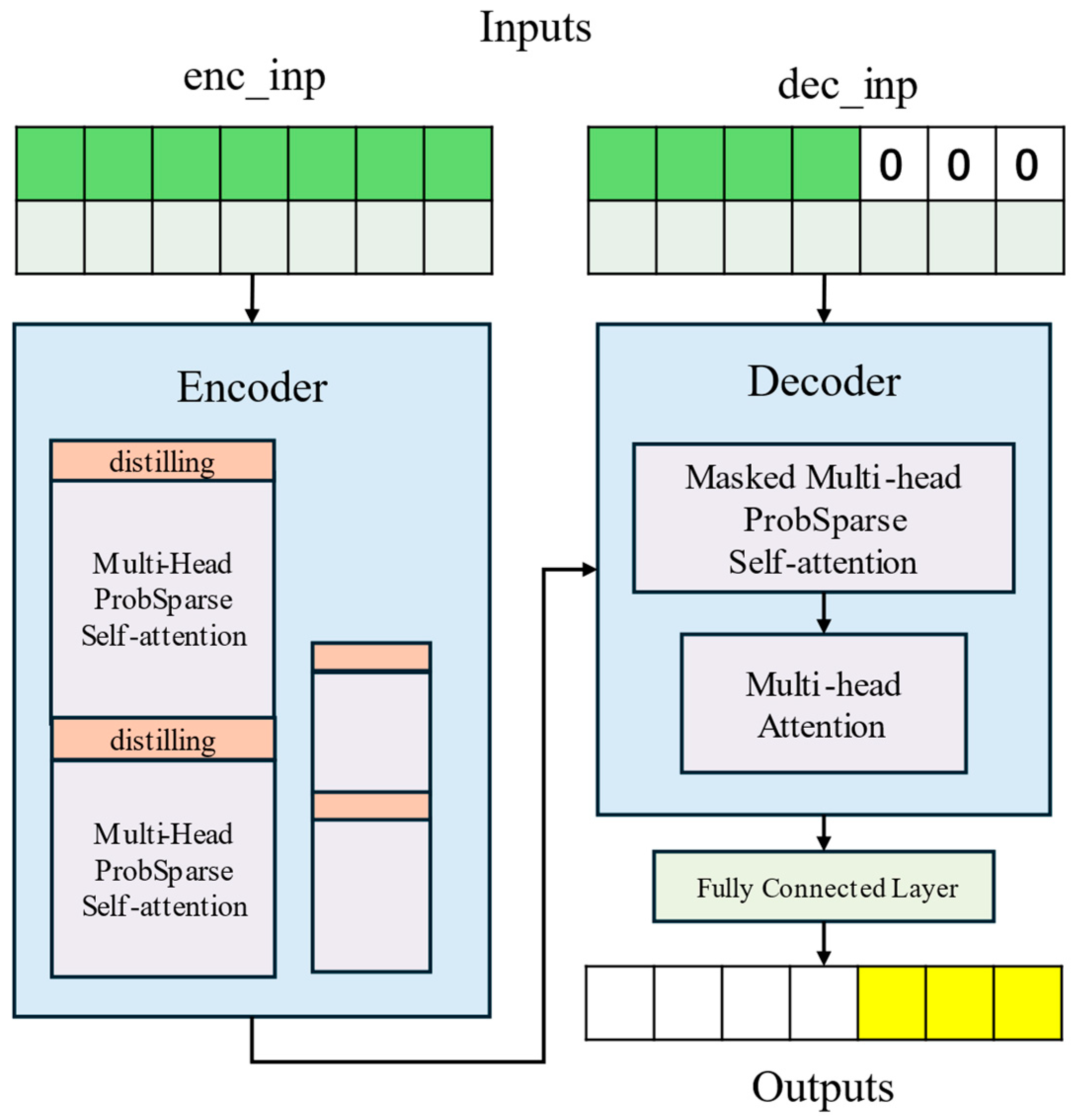
Informer is an efficient Transformer model designed for long-sequence time-series prediction, as illustrated in Figure 1. It aims to overcome the quadratic time complexity and high memory consumption of conventional Transformers when handling long sequences, as well as inherent limitations of the encoder–decoder architecture, thereby enhancing predictive capability and efficiency for long-sequence inputs and outputs.

The self-attention mechanism of the basic Transformer relies on standard dot-product operations, and this yields time and memory complexities that grow quadratically with sequence length. As multiple layers are stacked, memory usage further accumulates, making it difficult to process long inputs; meanwhile, the decoder’s autoregressive generation of predictions step by step causes a substantial slowdown in inference for long-horizon prediction. To break through these limitations, Informer introduces three key innovations [22].

First, the ProbSparse self-attention mechanism exploits the sparsity inherent in attention distributions to achieve efficient dependency alignment. Using a query sparsity metric to identify critical queries, it allows each key to attend only to a subset of dominant queries, thereby reducing per-layer time complexity and memory footprint while maintaining dependency alignment performance comparable to standard self-attention. The ProbSparse self-attention is defined as:

$$\mathcal{A}\left(Q,K,V\right)=\mathrm{Softmax}\left({\displaystyle \frac{\overline{Q}{K}^{\mathrm{\top }}}{\sqrt{d}}}\right)V$$

(1)

The sparsity metric is computed as the difference between the log-sum-exp and the arithmetic mean of a query’s scores over all keys; the formula is:

$$M\left(q_i,K\right)=\ln {\displaystyle \sum _{j=1}^{L_K}}{e}^{{\displaystyle \frac{q_i{k}_j^{\mathrm{\top }}}{\sqrt{d}}}}-{\displaystyle \frac{1}{L_K}}{\displaystyle \sum _{j=1}^{L_K}}{\displaystyle \frac{q_i{k}_j^{\mathrm{\top }}}{\sqrt{d}}}$$

(2)

Furthermore, the computation is simplified via a maximum-mean approximation to ensure numerical stability; the corresponding approximation is:

$$\overline{M}\left(q_i,K\right)=\underset{j}{\mathit{max}}\left\{{\displaystyle \frac{q_i{k}_j^{\top }}{\sqrt{d}}}\right\}-{\displaystyle \frac{1}{L_K}}{\displaystyle \sum _{j=1}^{L_K}}{\displaystyle \frac{q_i{k}_j^{\top }}{\sqrt{d}}}$$

(3)

Secondly, the self-attention distilling operation progressively filters dominant attention features layer by layer, effectively reducing the memory (space) complexity of stacked layers. After each stacked layer, this operation applies a one-dimensional convolution, ELU activation, and max pooling to halve the temporal dimension of the input sequence; its formulation is:

$$X_{j+1}^t=\mathit{MaxPool}\left(\mathit{ELU}\left(\mathit{Conv}\mathit{𝟣}d\left({\left[X_j^t\right]}_{AB}\right)\right)\right)$$

(4)

This design lowers the overall memory complexity and, by constructing stacked replicas with progressively halved input lengths and concatenating their outputs, enhances the model’s ability to handle ultra-long input sequences. Finally, the generative decoder replaces the step-by-step inference of the conventional encoder–decoder architecture with a single forward pass that completes long-horizon prediction. Its input is formed by concatenating a start token with placeholders for the target sequence; the formulation is:

$$X_{de}^t=\mathit{Concat}\left(X_{\mathit{token}}^t,X_0^t\right)\in R^{\left(L_{token}+L_y\right)\times d_{model}}$$

(5)

By leveraging masked multi-head attention to circumvent the autoregressive constraint, the model can directly produce the complete long-horizon prediction during both training and inference, substantially improving inference speed for long sequences.

Empirical results show that Informer significantly outperforms existing methods such as ARIMA, Prophet, LSTM, and DeepAR on multiple large-scale datasets (e.g., transformer temperature, electricity load, and meteorological data). Its prediction error increases more slowly with longer prediction horizons, and it demonstrates clear advantages in both inference speed and memory efficiency, validating its effectiveness and practicality for long-sequence time-series prediction [22]. These cross-domain results indicate that Informer has general advantages in scenarios characterized by long sequences, nonstationarity, and sparse critical events. For ROP prediction, this implies that the model can robustly capture a small number of key turning points over long well sections while maintaining scalable inference efficiency.

2.2. TCN

TCN is a general convolutional architecture for sequence prediction, designed to integrate best practices from modern convolutional networks into a concise and efficient starting point for sequence modeling. TCN is constructed within the broader Convolutional Neural Network (CNN) paradigm. CNNs exploit local connectivity and weight sharing to learn hierarchical features via convolutional kernels (1D for sequences, 2D/3D for images and volumes). Convolution in TCN is constructed to adapt to sequence data, preserving causality and long-range dependencies while retaining the efficiency of CNNs. It should be noted that TCN is not an entirely new architecture but rather a descriptive term for a family of architectures. Its core characteristics rest on two key principles: (1) the network adopts causal convolutions to prevent “leakage” of future information, meaning that the output at each time step depends only on the current and past inputs; and (2) it can accept sequences of arbitrary length and map them to output sequences of the same length, similar to the Recurrent Neural Network (RNN).

In sequence modeling, the model must predict outputs based on the historical portion of the input. Specifically, given an input sequence $(x_0,\dots ,x_T)$ and the corresponding output sequence $(y_0,\dots ,y_T)$, each $y_t$ is allowed to depend only on $(x_0,\dots ,x_t)$ and must not involve any “future” inputs $(x_{t+1},\dots ,x_T)$. This causal constraint is fundamental to sequence modeling. TCN enforces this constraint via causal convolutions, which can be summarized as “1-D Fully Convolutional Network (FCN) combined with causal convolution”: the 1-D FCN ensures that each hidden layer has the same length as the input layer by adding zero padding of length (kernel size − 1); the causal convolution guarantees that the output at time $t$ is computed by convolving only with elements at time $t$ and earlier in the previous layer, thereby completely avoiding contamination from future information.

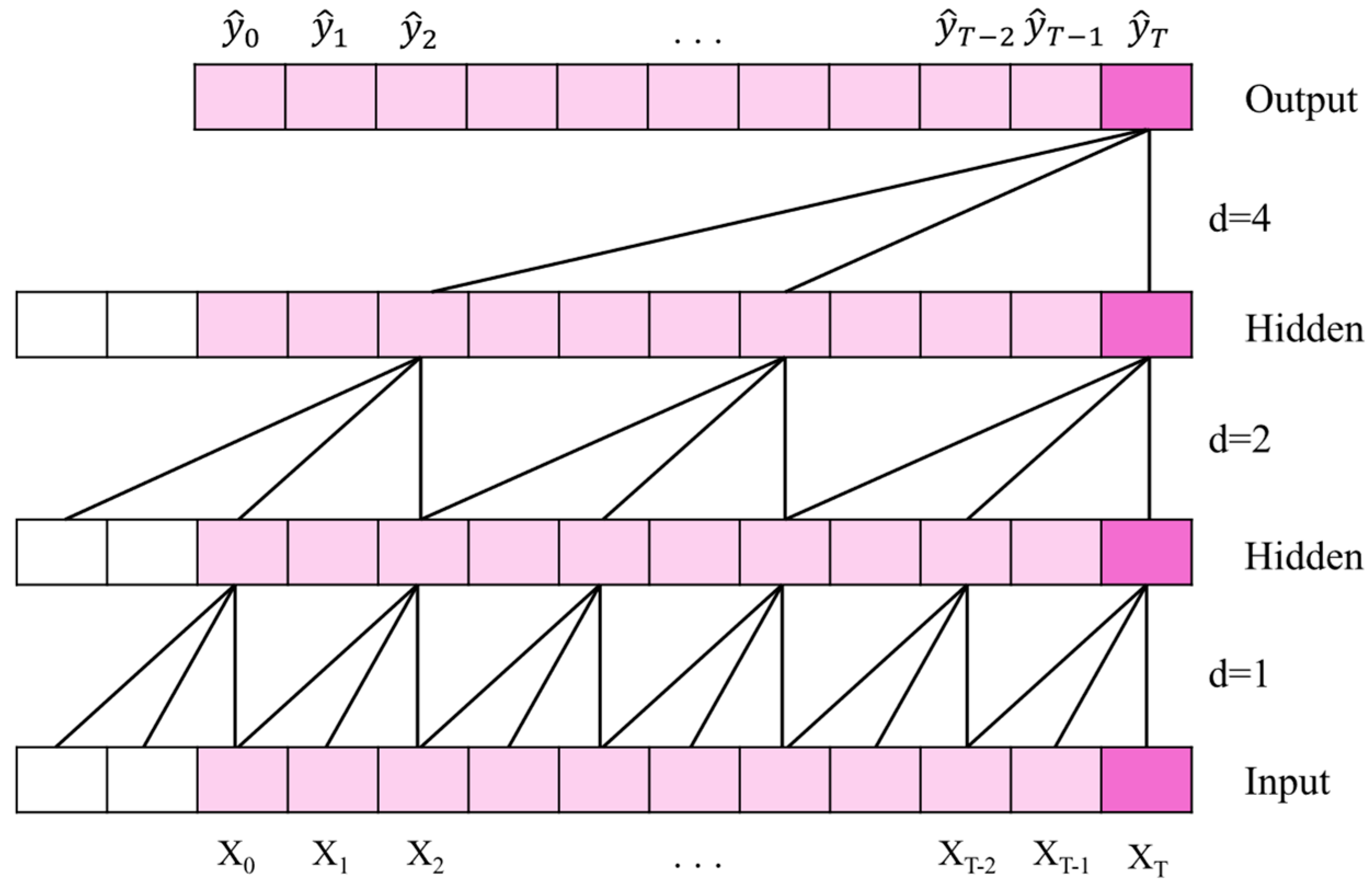
A basic causal convolution has a clear limitation: its effective history length grows linearly with network depth, which is inadequate for tasks requiring long-range historical context. To address this issue, TCN introduces dilated convolutions [23]. As illustrated in Figure 2, by inserting a fixed stride (the dilation factor) between kernel elements, the receptive field grows exponentially. The computation of a dilated convolution can be expressed as:

$$F\left(s\right)=\left(x{\ast }_{d}f\right)\left(s\right)={\displaystyle \sum _{i=0}^{k-1}}f\left(i\right)\cdot x_{s-d\cdot i}$$

(6)

where $d$ is the dilation factor and $k$ is the kernel size, while the term $s-d\cdot i$ reflects the backward traversal over historical inputs. In practice, the dilation factor typically increases exponentially with depth (e.g., $2^i$ at layer $i$), enabling deep networks to cover extremely long histories while ensuring that every input position within the receptive field is captured by the corresponding convolutional kernel.

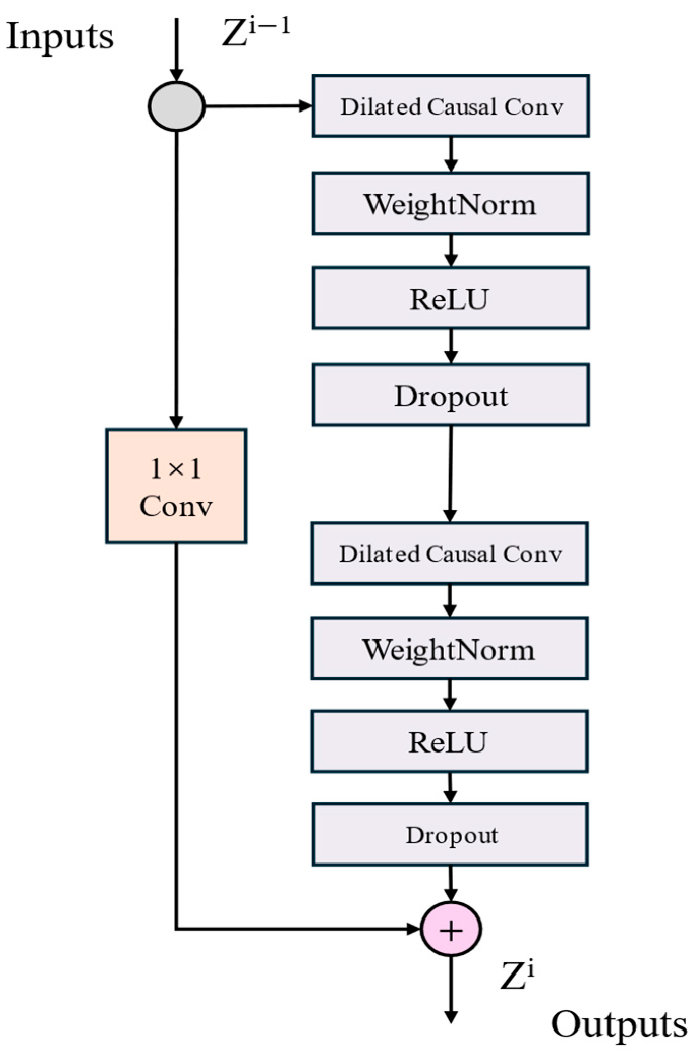
To stabilize the training of deep TCN and improve performance, residual connections are incorporated into the architecture [23]. As shown in Figure 3, each residual block contains two layers of dilated causal convolutions with ReLU activations in between. Weight normalization is applied to the convolutional kernels to accelerate training, and spatial dropout is added after each dilated convolution for regularization (randomly dropping entire channels during training). The computation of a residual block can be expressed as:

$$residual block=Activation\left(x+\mathcal{F}\left(x\right)\right)$$

(7)

where $\mathcal{F}\left(x\right)$ is a sequence of transformations. When the input and output dimensions differ, a 1 × 1 convolution is used to match dimensions and enable elementwise addition. This design allows each layer to learn a correction to the identity mapping rather than a full transformation, substantially enhancing the training stability of deep networks.

TCN offers several advantages for sequence modeling. In terms of parallelism, convolutions—with kernels shared across positions—allow entire long input sequences to be processed in parallel, eliminating the temporal dependencies of RNN and markedly improving training and evaluation efficiency. The receptive field can be flexibly controlled by adjusting the kernel size, dilation factor, or network depth, facilitating adaptation to different domains. The backpropagation path is decoupled from the temporal direction, mitigating the gradient explosion and vanishing issues common in RNN. Memory demand during training is relatively low, since kernels are shared within layers and backpropagation depends primarily on network depth; by contrast, gated mechanisms in RNN often lead to substantially higher memory usage. Moreover, similar to RNN, TCN can process input sequences of arbitrary length via sliding 1-D convolutional kernels, making it a practical replacement across diverse sequential data.

TCN also has limitations. During evaluation, RNN can generate predictions by maintaining only the hidden state and the current input, whereas TCN must retain the portion of the input sequence within the effective history (i.e., the receptive field), which can increase memory consumption. When transferring from domains with modest memory requirements to those demanding long-range temporal dependencies, an insufficient receptive field in the original TCN may degrade performance.

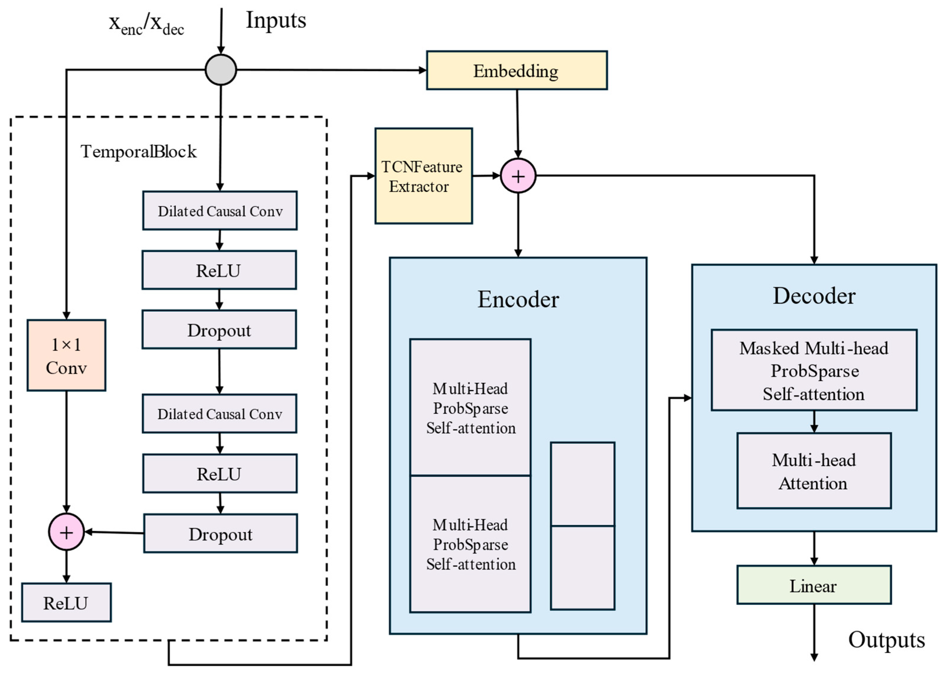
Overall, by organically combining causal convolutions, dilated convolutions, and residual connections, TCN demonstrates the potential to surpass traditional recurrent architectures (e.g., LSTM, GRU) in sequence modeling, providing a concise and efficient alternative. TCN focuses on short- to mid-term controllable operations and local dynamics, yielding a clean and robust local prior; on this basis, Informer captures sparse yet critical long-range dependencies. Together, they complement each other and support accurate multi-length, long-span ROP prediction [24,25].

3. Methodology

3.1. TCN–Informer

To leverage deep sequential data for ROP prediction, this study proposes the TCN–Informer architecture shown in Figure 4. The TCN–Informer model is an organic integration of the TCN and the Informer, aiming to combine the TCN’s efficient capture of local sequential features with the Informer’s strength in modeling long-range dependencies, thereby further improving the accuracy and efficiency of long-sequence time-series prediction. The model retains the Informer’s core innovations for long-horizon prediction while introducing a TCN module to enhance local feature extraction; however, this study removes normalization within the TCN residual blocks and the distilling operation in the Informer encoder, yielding better predictive performance.

In the proposed TCN–Informer architecture, the decisions to remove WeightNorm from the TCN and the encoder’s distilling layer are theoretically motivated by considerations of signal preservation and gradient propagation. Within causal, dilated convolutional residual paths, WeightNorm reparameterizes filters as a unit-norm direction scaled by a gain. Under causal padding, this reparameterization alters the amplitude response near boundaries and compresses local magnitude variations, thereby suppressing high-frequency transients and short-term contrasts that are discriminative for abrupt ROP changes. Residual blocks already stabilize the dynamics, and LayerNorm in the Informer stack provides token-wise statistical stability, so additional normalization in the TCN is unnecessary and can distort magnitude-phase characteristics. On the Informer side, the encoder’s distilling layer acts as a low-pass filter—reducing token density, introducing phase lag, and discarding fine temporal detail—precisely the information the TCN is designed to enhance. It also thins gradients over time, weakening supervision for early positions and hindering the alignment between encoder features and decoder queries. Consequently, removing WeightNorm from the TCN and the distilling layer from the Informer preserves high-frequency content, maintains consistent gradient scales along residual paths, and reduces residual error and phase lag in multi-length ROP prediction, thereby improving overall accuracy and stability.

The overall architecture consists of four key components: input embedding and TCN-based feature extraction, the Informer encoder, the Informer decoder, and the output projection. Let the batch size be $B$, the encoder length be the input sequence length $L_{enc}$, the decoder length be the sum of the label and prediction sequence lengths $L_{dec}$, the feature dimension be $C$, and the model dimension be $d_{model}$.

3.1.1. Input Embedding and TCN-Based Feature Extraction

The input embedding module maps the raw input sequence into a high-dimensional feature space and injects position information to capture depth-wise positional order; the TCN feature extraction module further mines local depth patterns via causal convolutions and residual structures. Their outputs are fused by addition to provide richer initial features for subsequent encoding.

The input embedding comprises token embedding and position embedding. The token embedding uses a 1-D convolution to map the channel dimension of the input sequence to the model dimension $d_{\mathrm{model}}$, achieving a high-dimensional transformation of the raw features, formulated as:

$$x_{enc}\in R^{B\times L_{enc}\times C}$$

(8)

$$x_{dec}\in R^{B\times L_{dec}\times C}$$

(9)

$$y_{Token}={Conv1d\left(x^T\right)}^T$$

(10)

where the internal transpose is a dimension reordering of the input sequence (from $\left[B,L,C\right]$ to $\left[B,C,L\right]$). $x$ can be $x_{enc}$ or $x_{dec}$. $\mathit{Conv}\mathit{𝟣}d$ is a one-dimensional convolution with kernel size 3, stride 1, and circular padding of 1. the external transpose reorders dimensions back (from $\left[B,d_{\mathrm{model}},L\right]$ to $\left[B,L,d_{\mathrm{model}}\right]$).

The position embedding uses sine and cosine functions to generate positional encodings that capture depth-wise positional information, given by:

$$y_{\mathit{Position}}=\left\{\begin{array}{l} sin\left({\displaystyle \frac{i}{{\mathrm{10,000}}^{2k/d_{model}}}}\right)\hspace{0.25em}, j=2k\\ cos\left({\displaystyle \frac{i}{{\mathrm{10,000}}^{2k/d_{model}}}}\right)\hspace{0.25em}, j=2k+1\hspace{0.25em}\hspace{0.25em}\hspace{0.25em}\hspace{0.25em}\end{array}\right.$$

(11)

where $i$ is the index of a depth point in the sequence, $j$ is the feature dimension index, and $k$ is $j//2$.

The final output of the input embedding is the sum of the token and position embeddings followed by dropout regularization, formulated as:

$$y_{\mathit{Embedding}}=\mathit{Dropout}\left(y_{Token}+y_{\mathit{Position}}\right)$$

(12)

The TCN feature extraction module captures local dependencies in the input depth sequence through multi-layer causal dilated convolutions and residual connections. Its core components are the causal dilated convolution and the residual block.

The causal dilated convolution ensures that the output at each depth position depends only on the current and shallower depths, thereby preventing leakage of future information. Sequence length is preserved via left zero padding, formulated as:

$$y_{\mathit{DilatedCausalConv}\mathit{𝟣}d}=\mathit{Conv}\mathit{𝟣}d\left(\mathit{PadLeft}\left(x,\left(k-1\right)\cdot d\right)\right)$$

(13)

where $x$ is the input feature tensor to the causal dilated convolution, $k$ is the kernel size, $d$ is the dilation factor, and $\mathit{PadLeft}\left(x,p\right)$ pads $p$ zeros on the left of the sequence. $\mathit{Conv}\mathit{𝟣}d$ is a 1-D pointwise convolution with kernel size 1 (used for residual dimension matching when input and output channels differ).

Each residual block (TemporalBlock) contains two layers of causal dilated convolutions combined with ReLU activation, dropout regularization, and residual connections, formulated as:

$$x_1=\mathit{Dropout}\left(\mathit{ReLU}\left(y_{\mathit{DilatedCausalConv}\mathit{𝟣}d}\left(x\right)\right)\right)$$

(14)

$$\mathcal{F}\left(x\right)=\mathit{Dropout}\left(\mathit{ReLU}\left(y_{\mathit{DilatedCausalConv}\mathit{𝟣}d}\left(x_1\right)\right)\right)$$

(15)

$$y_{\mathit{TemporalBlock}}=\mathit{ReLU}\left(\mathcal{F}\left(x\right)+\mathit{Conv}\mathit{𝟣}d\left(x\right)\right)$$

(16)

The TCN feature extractor stacks multiple residual blocks to perform deep mining of local features, with output:

$$y_{\mathit{TCNFeatureExtractor}}\left(x\right)=\mathit{TCNLayers}\left(Conv1d{\left(x^T\right)}^T\right)$$

(17)

where $\mathit{Conv}\mathit{𝟣}d$ is a 1-D pointwise convolution with kernel size 1 (mapping input channels to $d_{\mathrm{model}}$). Transpose is used for dimensionality transformation, and $\mathit{TCNLayers}$ is a stack of TemporalBlock.

The outputs of the input embedding and the TCN feature extractor are fused by addition and used as the inputs to the encoder and decoder, formulated as:

$$y_{\mathit{enc}\_\mathit{inp}}=y_{\mathit{Embedding}}\left(x_{\mathit{enc}}\right) + y_{\mathit{TCNFeatureExtractor}}\left(x_{\mathit{enc}}\right)$$

(18)

$$y_{\mathit{dec}\_\mathit{inp}}=y_{\mathit{Embedding}}\left(x_{\mathit{dec}}\right)+y_{\mathit{TCNFeatureExtractor}}\left(x_{\mathit{dec}}\right)$$

(19)

where $x_{\mathrm{enc}}$ and $x_{\mathrm{dec}}$ are the raw inputs to the encoder and decoder, respectively. $\mathit{Embedding}$ is the input embedding module, and $\mathit{TCNFeatureExtractor}$ is the TCN feature extraction module.

3.1.2. Informer Encoder

The encoder models long-range dependencies over the fused input features. Its core component is an encoder layer based on the ProbSparse self-attention mechanism, which, through multi-layer stacking, captures global dependencies by exploiting sparsity in attention distributions, thereby reducing computational complexity while preserving dependency alignment over depth sequences. Each encoder layer consists of a ProbSparse self-attention sublayer and a convolutional sublayer, with residual connections and layer normalization to enhance feature propagation; the formulation is:

$$x_1=x+\mathit{Dropout}\left(\mathit{AttentionLayer}\left(x,x,x\right)\right)$$

(20)

$$x_2=LayerNorm\left(x_1\right)$$

(21)

$$x_3=x_2+Dropout\left(Conv2{\left(\mathit{Dropout}\left(GELU\left(Conv1\left(x_2^T\right)\right)\right)\right)}^T\right)$$

(22)

$$y_{EncoderLayer}\left(x\right)=LayerNorm\left(x_3\right)$$

(23)

where $x$ is the fused sequence $y_{\mathit{enc}\_\mathit{inp}}$. $\mathit{AttentionLayer}$ is the ProbSparse self-attention layer. $\mathit{Conv}\mathit{𝟣}$ and $\mathit{Conv}\mathit{𝟤}$ are 1-D pointwise convolutions with kernel size 1 (mapping dimensions to $d_{\mathrm{ff}}$ and back to $d_{\mathrm{model}}$, respectively).

The encoder stacks multiple EncoderLayer modules to produce the final features, formulated as:

$$y_{\mathit{enc}\_\mathit{out}}=\mathit{Encoder}\left(y_{\mathit{enc}\_\mathit{inp}}\right)$$

(24)

3.1.3. Informer Decoder

The decoder receives the fused decoder input features together with the encoder outputs. It models intra-dependencies within the output depth sequence and the associations with the input depth sequence via self-attention and cross-attention, generating predictive features. Each decoder layer comprises a self-attention sublayer, a cross-attention sublayer, and a convolutional sublayer; the formulation is:

$$x_1=x+\mathit{Dropout}\left(\mathit{SelfAttentionLayer}\left(x,x,x\right)\right)$$

(25)

$$x_2=LayerNorm\left(x_1\right)$$

(26)

$$x_3=x_2+Dropout\left(CrossAttentionLayer\left(x_2,\mathit{\text{enc\_out}},\mathit{\text{enc\_out}}\right)\right)$$

(27)

$$x_4=LayerNorm\left(x_3\right)$$

(28)

$$x_5=x_4+Dropout\left(Conv2{\left(Dropout\left(GELU\left(Conv1\left(x_4^T\right)\right)\right)\right)}^T\right)$$

(29)

$$y_{DecoderLayer}\left(x,y_{\mathit{enc}\_\mathit{out}}\right)=LayerNorm\left(x_5\right)$$

(30)

where $x$ is the fused sequence $y_{\mathit{dec}\_\mathit{inp}}$. $\mathit{SelfAttentionLayer}$ is the self-attention layer with a causal mask (to prevent future information leakage), and $\mathit{CrossAttentionLayer}$ is the cross-attention layer (to model associations with the encoder outputs).

The decoder stacks multiple DecoderLayer modules to produce the predictive features:

$$y_{\mathit{dec}\_\mathit{out}}=\mathit{Decoder}\left(y_{\mathit{\text{dec\_inp}}},y_{\mathit{\text{enc\_out}}}\right)$$

(31)

3.1.4. Output Projection

The decoder’s output features are mapped to the target dimension by a linear projection layer to obtain the final predictions:

$$\widehat{y}=\mathit{Linear}\left(y_{\mathit{dec}\_\mathit{out}\left[:,-L_y:,:\right]}\right)$$

(32)

where $L_y$ is the length of the predicted depth sequence, and $\mathit{Linear}$ is a linear transformation (mapping $d_{\mathrm{model}}$ to the target variable dimension).

Because the linear projection introduces no additional nonlinearity, it preserves the phase and amplitude alignment established by the decoder and avoids morphological distortion of sparse critical events such as formation boundaries. This property is particularly important for strongly nonstationary and phase-sensitive ROP sequences. During training, this study applies stepwise Mean Square Error (MSE) supervision at this output, enabling gradients to propagate directly and stably to the decoder representations and projection weights. During inference, first denormalize the outputs from the standardized domain to physical units and then apply lightweight engineering post-processing, achieving a better trade-off between abrupt response and smoothness.

3.1.5. Model Advantages

TCN–Informer combines the strengths of TCN and Informer: the causal dilated convolutions in TCN effectively capture local patterns among adjacent depth points, complementing the Informer’s global dependency modeling; the ProbSparse self-attention mechanism reduces time complexity; the generative decoder performs one-step prediction, improving efficiency for long sequences; and residual connections together with layer normalization mitigate training instability. In series prediction tasks—especially those featuring both local patterns and long-range dependencies—the proposed model delivers superior predictive accuracy and efficiency compared with single-model baselines.

3.2. Data Preprocessing

3.2.1. Outlier Handling and Resampling

During drilling, raw data are prone to duplication, anomalies, and uneven distributions due to strong nonlinearity in the drilling process, formation uncertainty, and sensor interference. These issues can amplify errors in data-driven models and affect engineering decisions. Duplicate records, arising from high-frequency sampling vibrations or transmission delays, undermine sequential coherence, increase computational noise, and introduce decision latency. Anomalies and noise can mislead model learning, magnifying prediction bias; if left unaddressed, model error rises significantly. Uneven data distributions across formations and operational stages can compromise generalization and leave critical low-ROP intervals underpredicted, increasing the cost of repeated modeling [26]. Therefore, deduplication, anomaly detection, and resampling are necessary to improve data quality and ensure the engineering applicability of the TCN–Informer hybrid model. The dataset is preprocessed in four steps:

Step 1: Deduplication. To address potential duplicate sensor entries, group by unique depth values and compute the mean for each feature within each group, ensuring a consistent baseline for analysis.

Step 2: Sliding-window quantile detection. Within a 20 m window, use the interquartile range (IQR) to determine the normal-range boundaries of feature parameters and remove values that fall outside this range.

Step 3: Secondary anomaly detection. Apply the Isolation Forest algorithm to the data after the quantile-based filtering. A sample is deemed anomalous and removed if its anomaly score $\xi \left(x\right)$ exceeds a certain threshold, thereby improving the precision of anomaly identification.

Step 4: KNN resampling. Given the nonuniform distribution of raw data in the depth domain and sensor synchronization biases, adopt K equals 5 nearest-neighbor regression. Compute a weighted average using inverse squared distance as weights to resample data to 0.05 m intervals, providing regularized inputs for training sequential models.

In Step 1, the core operation is to group by depth and take the mean. For each unique depth d, compute the mean of each feature column f (e.g., weight on bit, standpipe pressure, surface torque, rotary speed, mud flow rate, mud density, hole diameter, hookload, vertical depth, the USROP gamma value, and ROP), denoted as $\overline{f_d}$; its formulation is:

$$\overline{f_d}={\displaystyle \frac{1}{n_d}}{\displaystyle \sum _{i=1}^{n_d}}{f}_{d_i}$$

(33)

where $d$ is the unique depth value, $n_d$ is the number of data points at depth $d$, $f_{d_i}$ is the i-th feature value at depth $d$, and $\overline{f_d}$ is the mean of feature f at depth $d$.

In Step 2, within a 20 m sliding window, compute the IQR of the feature values and derive the upper and lower bounds for outlier detection, denoted as $UpperBound$ and $LowerBound$.

$$Q1=P^{25}\left(X_w\right)$$

(34)

$$Q3=P^{75}\left(X_w\right)$$

(35)

$$IQR=Q3-Q1$$

(36)

$$LowerBound=Q1-1.5\times IQR$$

(37)

$$UpperBound=Q3+1.5\times IQR$$

(38)

where $X_w$ is the feature values within the window, and $P_k$ is the k-th percentile. Data points falling outside the interval [$LowerBound$, $UpperBound$] are excluded. In Step 3, build isolation trees on the quantile-filtered data to obtain the anomaly score $\xi \left(x\right)$:

$$\xi \left(x\right)=2^{-E\left(h\left(x\right)\right)/c\left(n\right)}$$

(39)

$$c\left(n\right)=2H\left(n-1\right)-2\left(n-1\right)/n$$

(40)

$$H\left(n-1\right)={\displaystyle \sum _{i=1}^{n-1}}{\displaystyle \frac{1}{i}}=1+{\displaystyle \frac{1}{2}}+{\displaystyle \frac{1}{3}}+\dots +{\displaystyle \frac{1}{n-1}}$$

(41)

where $h\left(x\right)$ is the path length from the root to the leaf for sample $x$, and $H\left(n-1\right)$ is the harmonic number. A sample with $\xi \left(x\right)$ exceeding 0.65 is classified as an outlier and excluded from subsequent use.

In Step 4, resampling refers to recomputing continuous sensor readings with respect to arbitrary indices. Using K equals 5 nearest-neighbor regression, resample the depth and other feature data $x\left(d\right)$ to 0.05 m intervals to obtain the resampled data $\widehat{x}\left(d\right)$, with the computation given by:

$$\widehat{x}\left(d\right)={\displaystyle \frac{{\sum }_{i=1}^K{w}_{i}x\left(d_i\right)}{{\sum }_{i=1}^K{w}_i}}$$

(42)

$$w_i={\displaystyle \frac{1}{{\left|d-d_i\right|}^2}}$$

(43)

where $d$ is the target depth and $d_i$ is the depths of neighboring points.

3.2.2. Feature Standardization and Label Denormalization

To eliminate inter-feature unit and scale differences, enhance training stability, and ensure general applicability of the model to ROP prediction, standardization parameters are computed separately for each well. Let the feature matrix be $x\in R^{I\times d}$ and the label sequence be $y\in R^I$. Column−wise z−score standardization is applied; in addition, the standardized label is concatenated as a one−dimensional auxiliary feature with the standardized features and fed into the model. A small constant $ϵ$ equals ${10}^{-8}$ is used to prevent divide-by-zero issues and ensure numerical stability.

Furthermore, the standardized label is concatenated as a one-dimensional auxiliary channel to the standardized features and fed to both the encoder and decoder. This design is motivated by the strong short-term autocorrelation in ROP: providing the model with a causal history of the target acts as a stabilizing signal. This signal regularizes attention and TCN filters during multi-length decoding, reduces covariate shift induced by well-specific scale differences, and empirically improves convergence by aligning the decoder’s conditioning with the true process dynamics. The approach is analogous to the known past target inputs commonly used in sequence forecasting.

Nevertheless, concatenating the label necessitates careful examination of information leakage. Primary risks include inadvertent exposure of future labels during training or inference, and leakage via normalization if statistics are computed on full well series containing the evaluation horizon. This implementation enforces strict causality: only historical labels within the encoder and decoder’s known segment are used, while future decoder positions are filled with the last observed frame rather than true future labels. Predictions are always denormalized and compared against the original ground truth.

For feature standardization, compute the mean ${\mu }_j$ and standard deviation ${\sigma }_j$ for the j-th feature column ($j=1,\dots ,d$). For label standardization, compute the mean ${\mu }_y$ and standard deviation ${\sigma }_y$ for $y$:

$${\stackrel{\sim }{x}}_{i,j}={\displaystyle \frac{x_{i,j}-{\mu }_j}{{\sigma }_j+ϵ}}$$

(44)

$${\stackrel{\sim }{y}}_i={\displaystyle \frac{y_i-{\mu }_y}{{\sigma }_y+ϵ}}$$

(45)

Finally, at each depth $i$, the model input vector ${\mathrm{z}}_i\in R^{d+1}$ is constructed by concatenating the standardized feature vector ${\stackrel{\sim }{\mathrm{x}}}_i$ and the standardized label ${\stackrel{\sim }{y}}_i$, i.e., ${\mathrm{z}}_i=[{\stackrel{\sim }{\mathrm{x}}}_i;{\stackrel{\sim }{y}}_i]$. The model outputs multi-length predictions ${\stackrel{\sim }{y}}_i$ in the standardized space. For performance evaluation and visualization, predictions must be denormalized back to the original physical units. All evaluation metrics are computed on the denormalized predictions ${\widehat{y}}_i$ and the original ground-truth labels $y_i$.

$${\widehat{y}}_i={\stackrel{\sim }{y}}_i{\sigma }_y+{\mu }_y$$

(46)

4. Results

4.1. Data Processing

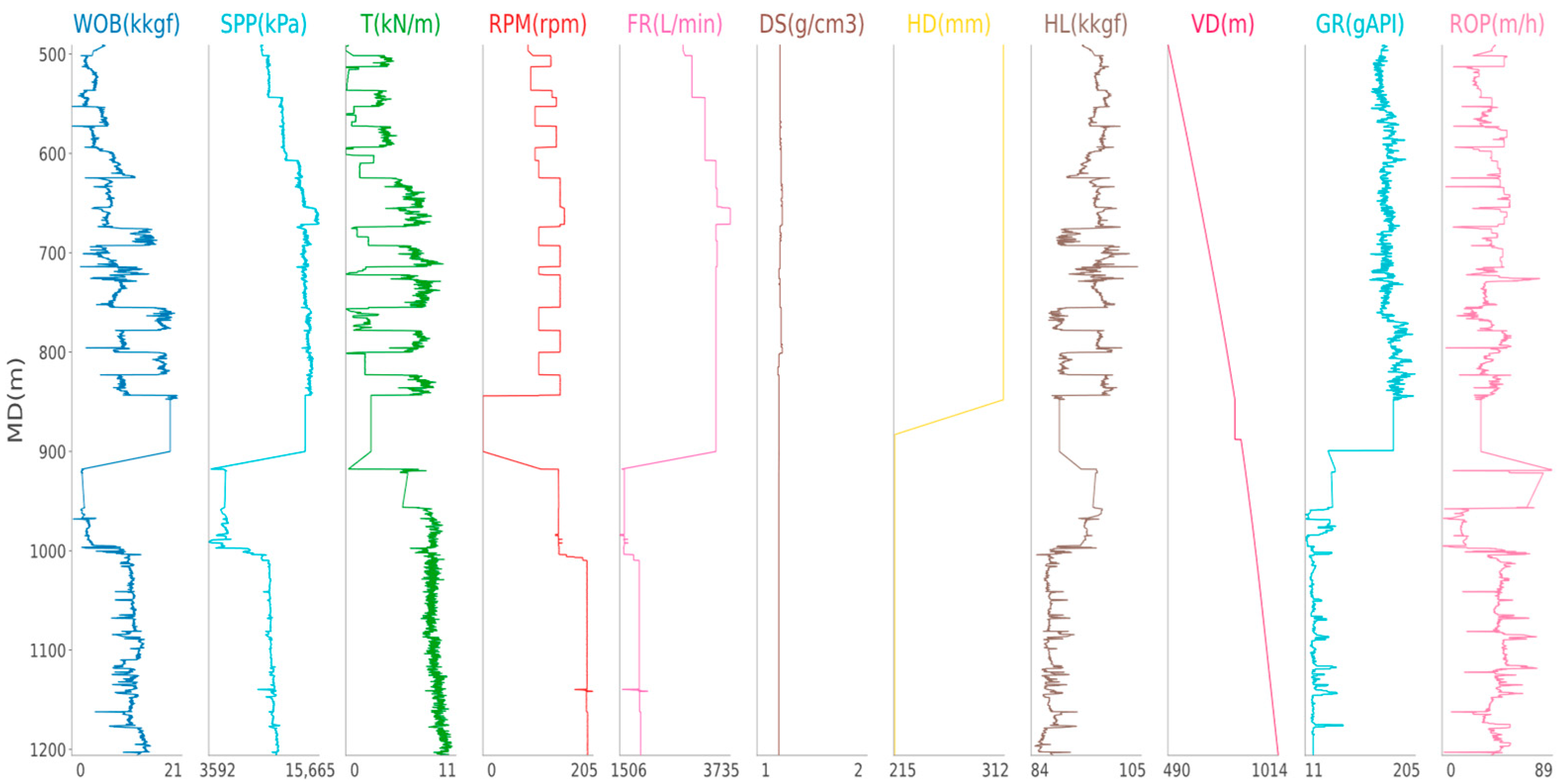
The drilling data used in this study come from the University of Stavanger Rate of Penetration (USROP) dataset constructed by Tunkiel et al. [27]. The dataset comprises nearly 200,000 sample records from seven wells and covers 12 common drilling attributes, including measured depth (MD), weight on bit (WOB), standpipe pressure (SPP), surface torque (T), rotary speed (RPM), mud flow rate (FR), mud density (DS), hole diameter (HD), hookload (HL), vertical depth (VD), the USROP gamma value (GR), and ROP. To evaluate the performance of TCN–Informer, this study selected three files from the USROP dataset: USROP_A 0 N-NA_F-9_Ad, USROP_A 2 N-SH_F-14d, and USROP_A 4 N-SH_F-15Sd, hereafter referred to as Well #1, Well #2, and Well #3. To visually illustrate parameter types, lengths, and variations, this paper selects Well #1 for detailed parameter presentation. Data formats for other wells follow the same pattern as Well #1.

Table 1. Drilling data for Well #1.

Parameter	Unit	Minimum	Maximum	Average
MD	m	491.033	1206.000	844.155
WOB	kkgf	0.005	20.102	9.289
SPP	kPa	3592.720	15,664.400	11,562.100
T	kN/m	0.014	10.616	5.937
RPM	rpm	0	204.170	143.320
FR	L/min	1506.520	3734.570	2714.110
DS	g/cm3	1.190	1.230	1.207
HD	mm	215.900	311.150	269.962
HL	kkgf	84.727	104.304	92.707
VD	m	490.760	1013.140	781.324
GR	gAPI	11.270	204.761	103.791
ROP	m/h	0.549	88.441	39.101

summarizes Well #1’s basic information, including the unit, minimum value, maximum value, and average value for each parameter. Figure 5 displays how each drilling parameter (WOB, SPP, T, RPM, etc.) varies with depth, revealing the nonlinear relationships between parameters during the drilling process. After preprocessing the features and labels for each well, the processed data were used for model training and evaluation.

4.2. Evaluation Metrics

This study adopts MAE, RMSE, 95th MAE, 95th RMSE, and R² as the core metrics to evaluate predictive performance.

$$MAE={\displaystyle \frac{1}{n}}\sum _{i=1}^n\left|y_i-{\widehat{y}}_i\right|$$

(47)

$$RMSE=\sqrt{{\displaystyle \frac{1}{n}}\sum _{i=1}^n(y_i-{\widehat{y}}_i{)}^2}$$

(48)

$$R^2=1-{\displaystyle \frac{{\sum }_{i=1}^n(y_i-{\widehat{y}}_i{)}^2}{{\sum }_{i=1}^n(y_i-\overline{y}{)}^2}}$$

(49)

where $n$ is the number of samples, $y_i$ is the ground-truth value of the i-th sample, ${\widehat{y}}_i$ is the model’s prediction for the i-th sample, and $\overline{y}$ is the mean of the ground-truth values across all samples.

MAE measures the average magnitude of the absolute differences between predictions and ground truth, with a range of [0, +∞). Compared with RMSE, MAE is less sensitive to outliers. A smaller MAE indicates higher predictive accuracy. RMSE quantifies the typical magnitude of the differences between predictions and ground truth, with a range of [0, +∞). RMSE is the square root of MSE and is more sensitive to larger errors. A smaller RMSE indicates higher predictive accuracy. R² assesses, from a statistical perspective, the extent to which the model explains the variability of the target variable, with a range of (−∞, 1]. Values of R² closer to 1 indicate that the model explains a greater proportion of the variance in the target variable and achieves a better overall fit between predictions and observations.

The 95th MAE and 95th RMSE, respectively, represent the mean absolute error and root mean square error for all values exceeding the fast jump threshold ($\gamma$). Calculated using the same methodology as MAE and RMSE, they can be derived by identifying the indices of fast jump points. Through these two metrics, model predictions can avoid long-term saturation values masking underestimation caused by rapid jumps, thereby effectively evaluating each model’s predictive performance at rapid jump points.

$$g_i=\left|{\displaystyle \frac{y_i-y_{i-1}}{d_i-d_{i-1}}}\right|$$

(50)

$$\gamma =Q_{95}\left(\{g_i\}\right)$$

(51)

$$S=\left\{i\mid g_i\ge \gamma \right\}$$

(52)

where $y_i$ is the ground-truth value of the i-th sample, $d_i$ is the depth for the i-th sample, $g_i$ is the rate of change in the i-th sample. $\gamma$ is the fast jump threshold, $Q_{95}$ is the 95-th percentile, and $S$ is the indices of fast jump points.

4.3. Parameter Settings and Hyperparameter Search

Parameter tuning plays a critical role in optimizing model performance, as demonstrated by related studies. In quantum differential evolution algorithms for constrained capacitated vehicle routing problems, hyperparameter calibration directly influences convergence speed and routing optimization quality [28]. In business process management, parameter configuration affects resource allocation efficiency and workload balancing effectiveness [29]. Consequently, systematic parameter setting and hyperparameter search are indispensable for balancing model complexity, training stability, and predictive accuracy. To balance modeling efficiency with the ability to capture sequence dependencies, this study configures the encoder input length, the decoder’s known-segment length, and the prediction length as specified in

Table 2. Hyperparameter Settings.

Parameter	Settings
Input dimension	11
Optimizer	Adam
Learning rate	1 × 10−5~1 × 10−3
Beta	0.9~0.999
Batch size	128
Number of Optuna hyperparameter searches	20
Hyperparameter search patience	3
Epochs per chunk	2
Cold start windows	12
Smooth early windows	5
Smooth alpha	0.6
Window size	10 × Input length
Sliding length	Prediction length
Input length	4 × Prediction length
Label length	2 × Prediction length
Prediction length	48/24/12/6/3
Model dimension	128~512
Number of attention heads	2/4/8
Number of encoder blocks	1~3
Number of decoder blocks	1~2
Fully connected network dimension	256~1024
Dropout coefficient	0.0~0.3
TCN layers	1~4
TCN kernel size	3/5/7

. This study concatenates the target variable with the raw features to strengthen the sequential signal. Training uses mini-batches and a chunked schedule, with multiple iterations per chunk and early stopping to limit overfitting. This study adopts Adam with weight decay, and selects the learning rate via automated hyperparameter search. To mitigate early-stage instability, this study enables a cold start over the first few windows and applies exponential moving-average smoothing to early predictions.

Hyperparameter search follows Optuna’s Bayesian optimization and uses MSE as the validation loss function. During hyperparameter tuning, the constructed sequence dataset is randomly split into training (90%) and validation (10%) subsets. No separate test set is utilized, and model selection is based on validation loss. The search space covers, for Informer, the model dimension, number of attention heads, numbers of encoder and decoder layers, feed-forward dimension, and dropout; and for TCN, the depth (number of levels) and kernel size. This study runs a bounded number of trials to strike a practical balance between efficiency and effectiveness.

4.4. Sliding Window

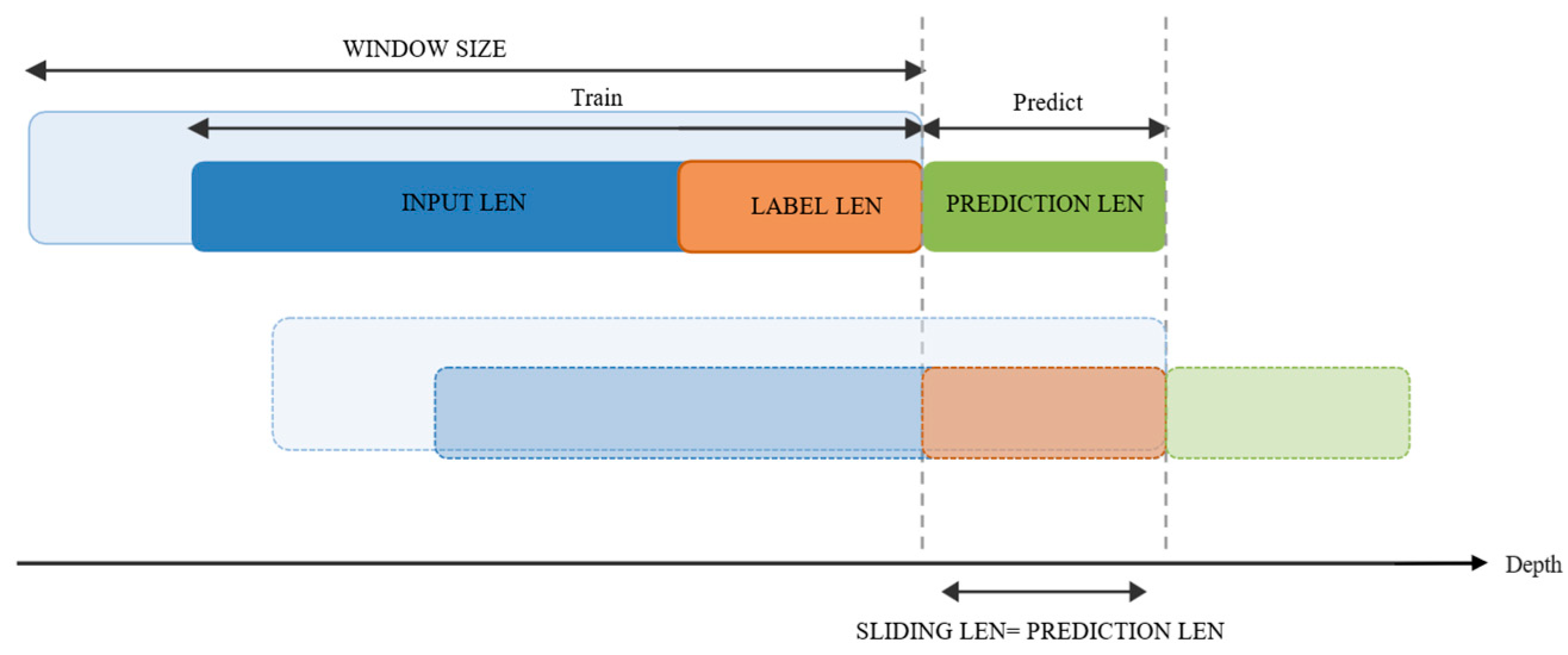
The sliding window is the core mechanism for constructing series samples and enabling continual learning. As shown in Figure 6, during training this study samples the current window to form the encoder input, the decoder’s known segment, and the prediction labels. During inference, the window advances by the prediction length (equal to the sliding length) and incorporates newly observed ground-truth values into subsequent windows.

This study sets the window size as an integer multiple of the input length to preserve short-term fluctuations and mid-term trends. To avoid distribution shift from uninformed padding, the decoder’s future segment uses a last-frame copy strategy to populate placeholder inputs. This design reduces memory footprint and computational load by limiting window length, while it expands the receptive field through multi-layer causal dilated convolutions in the TCN module to capture longer-period dependencies. Together, rolling prediction and cold-start smoothing improve adaptation to distribution drift and suppress early prediction volatility.

4.5. TCN–Informer vs. Informer ROP Prediction Comparison

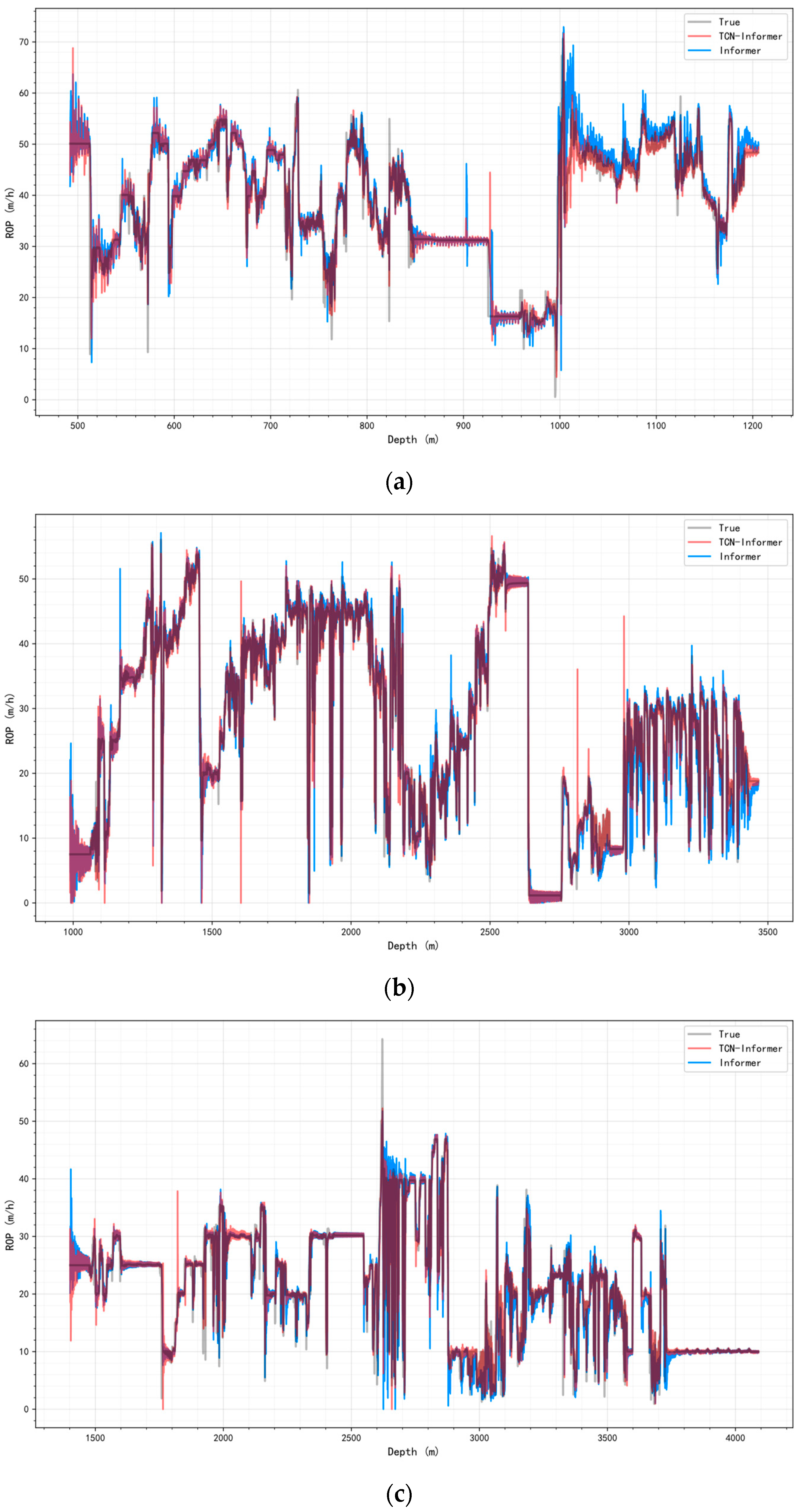
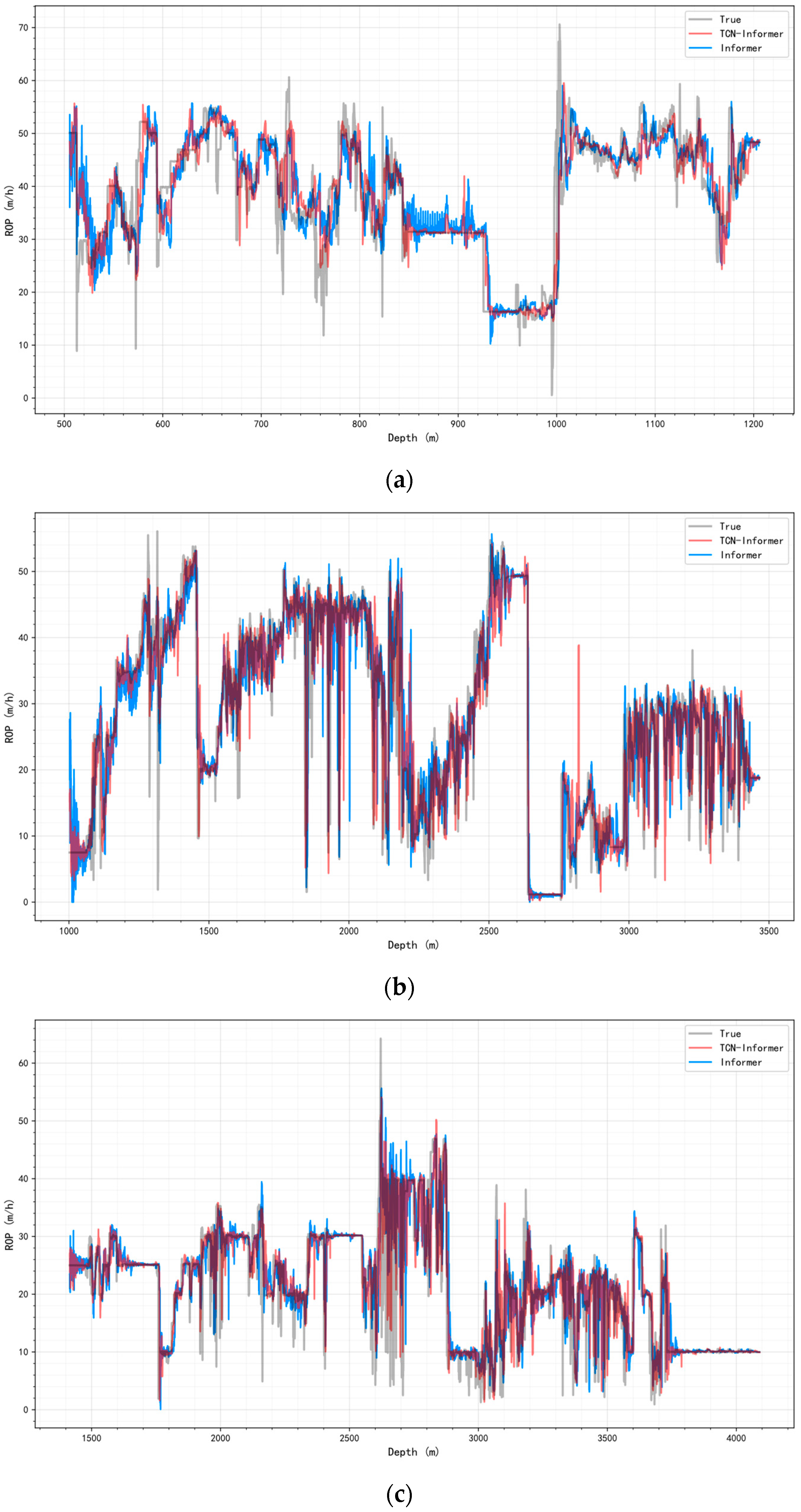
This study feeds the processed features and labels into two models: TCN–Informer and the baseline Informer. A sliding window is used to perform continual ROP prediction. Figure 7 shows a short-sequence setting (input 12, predict 3). Figure 8 shows a long-sequence setting (input 192, predict 48). Both figures demonstrate the ROP prediction performance of TCN–Informer and Informer. TCN–Informer achieves prediction results closer to actual ROP under both short-sequence and long-sequence settings, exhibiting superior long-term fitting and local noise suppression capabilities.

Across sequence setting, segment lengths, and well conditions, TCN–Informer generally performs better and more consistently. For Well #1, in intervals with dense high-frequency perturbations and local spikes (500–520 m and 985–1005 m), TCN–Informer responds faster to abrupt changes. It shows smaller phase lag at turning points and produces peak-trough amplitudes and arrival times closer to the ground truth. In near-steady or slowly varying intervals (approximately 1005–1180 m), its predictions are smoother, with less overshoot, smaller residual fluctuations, and slower error accumulation as the prediction horizon extends.

This study observes the same pattern in Well #2 and Well #3. In segments with high-frequency perturbations and local spikes (1950–2150 m in Well #2; 2950–3120 m in Well #3), TCN–Informer suppresses noise-induced oscillations and limits over-tracking. In near-steady segments (2600–2700 m in Well #2; 3800–4100 m in Well #3), it maintains trend continuity and stable amplitudes.

These results align with the model design. The TCN branch, through causal dilated convolutions, rapidly captures short-period mechanical vibrations and local inertia, providing a clean short-term prior for the Informer. The Informer, using sparse attention, focuses on distant key dependencies, enabling accurate alignment at abrupt boundaries and over long ranges. As a result, across wells with varying segment lengths and operating conditions (Well #1, Well #2, and Well #3), TCN–Informer effectively fuses short- and long-term information. Compared with the basic Informer, it produces smaller residuals and weaker phase lag, demonstrating strong adaptability to diverse well types and conditions.

4.6. Ablation Study on TCN and Informer Components

To analyze the independent contributions of TCN and Informer components to overall performance, this study separately employed TCN and Informer as standalone models for ROP prediction under consistent experimental conditions, obtaining their evaluation metrics as shown in

Table 3. Evaluation metrics of ablation study at different sequence lengths.

Methods	Input Len	Prediction Len	MAE	RMSE	95th MAE	95th RMSE	R2
TCN	192	48	4.160	8.797	6.603	9.422	0.371
	96	24	2.857	6.158	5.780	8.505	0.698
	48	12	2.050	4.770	4.868	7.280	0.828
	24	6	1.565	4.305	3.950	6.010	0.861
	12	3	0.894	1.960	3.033	4.760	0.970
Informer	192	48	3.458	5.817	6.815	9.745	0.741
	96	24	2.620	4.766	5.979	8.655	0.825
	48	12	1.987	3.901	5.357	7.930	0.884
	24	6	1.560	3.142	4.669	7.037	0.923
	12	3	1.365	2.569	4.125	6.145	0.945
TCN–Informer (this study)	192	48	3.052	5.328	6.350	9.112	0.783
	96	24	2.321	4.323	5.744	8.454	0.856
	48	12	1.726	3.502	5.055	7.572	0.906
	24	6	1.314	2.763	4.111	6.335	0.940
	12	3	1.033	2.094	3.335	5.211	0.965

.

This ablation study reveals the distinct and complementary contributions of TCN and the Informer model. In both the long-sequence and short-sequence settings, Informer alone consistently achieves lower MAE and RMSE than TCN while maintaining higher R² values, reflecting its superior modeling capability for long-range dependencies. Conversely, TCN alone achieves lower 95th MAE and 95th RMSE than Informer across all sequence settings, with optimal performance across all metrics in the short-sequence setting (input 12, predict 3), indicating its superiority in capturing local high-frequency dynamics. The TCN–Informer achieves optimal performance in the long-sequence setting (input 192, predict 48 and input 96, predict 24), reducing MAE, RMSE, 95th percentile MAE, and 95th percentile RMSE while attaining the highest R². In the short-sequence setting (input 48, predict 12 and input 24, predict 6), it also delivers the best MAE, RMSE, and R² values. Overall, Informer outperforms TCN on metrics in the long-sequence setting, while TCN outperforms Informer on metrics in the short-sequence setting and at fast jump points. This validates a complementary mechanism: TCN’s causal convolutions provide clear short-term prior information, while Informer’s sparse attention coordinates long-range dependencies, thereby enhancing model accuracy.

4.7. TCN–Informer vs. Other Sequence Models ROP Prediction Comparison

To compare TCN–Informer with other sequence models for ROP prediction, this study evaluates TCN–Informer, Informer, LSTM, GRU, and Transformer on Well #1, Well #2, and Well #3, and reports the metrics MAE, RMSE, 95th MAE, 95th RMSE, and R² for ROP. This study also analyzes representative segments from Well #1. The results are summarized in

Table 4. Evaluation metrics of different models at different sequence lengths.

Methods	Input Len	Prediction Len	MAE	RMSE	95th MAE	95th RMSE	R2
LSTM	192	48	4.960	7.248	7.425	10.501	0.596
	96	24	3.972	6.425	6.841	9.662	0.676
	48	12	3.261	5.612	6.279	8.823	0.753
	24	6	2.680	4.933	6.096	8.916	0.807
	12	3	2.666	4.875	6.120	8.623	0.815
GRU	192	48	5.142	7.477	7.572	10.748	0.571
	96	24	3.908	6.307	7.024	10.128	0.683
	48	12	2.976	5.136	6.090	8.662	0.791
	24	6	2.500	4.571	5.907	8.465	0.835
	12	3	2.150	4.190	5.486	7.996	0.858
Transformer	192	48	4.084	6.527	7.176	10.331	0.671
	96	24	3.542	5.935	6.982	10.066	0.721
	48	12	2.889	5.208	6.365	9.354	0.789
	24	6	2.815	4.981	5.987	8.745	0.809
	12	3	2.721	5.073	6.148	8.825	0.796
Informer	192	48	3.458	5.817	6.815	9.745	0.741
	96	24	2.620	4.766	5.979	8.655	0.825
	48	12	1.987	3.901	5.357	7.930	0.884
	24	6	1.560	3.142	4.669	7.037	0.923
	12	3	1.365	2.569	4.125	6.145	0.945
TCN–Informer (this study)	192	48	3.052	5.328	6.350	9.112	0.783
	96	24	2.321	4.323	5.744	8.454	0.856
	48	12	1.726	3.502	5.055	7.572	0.906
	24	6	1.314	2.763	4.111	6.335	0.940
	12	3	1.033	2.094	3.335	5.211	0.965

.

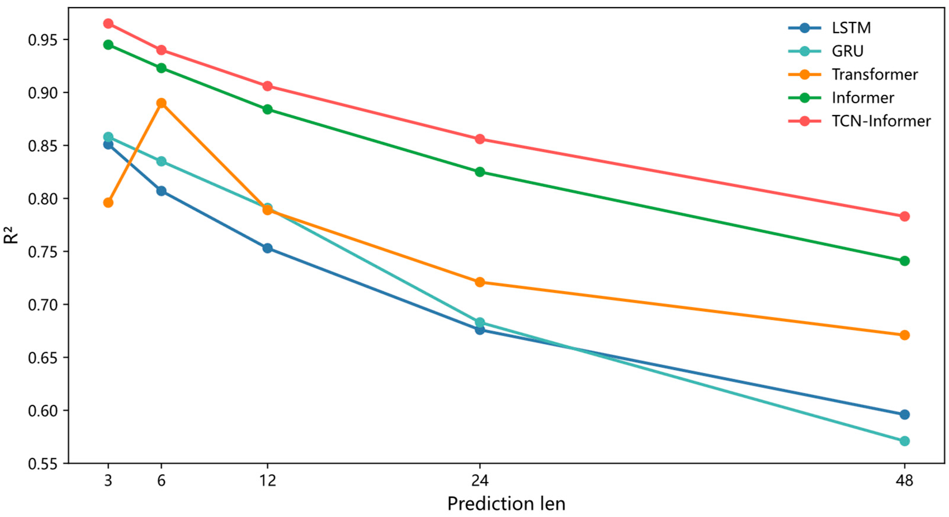
The comparative experiments span multiple settings, from short input with short prediction to long input with long prediction. Table 4 and Figure 9 show a clear trend: in most settings, TCN–Informer achieves lower MAE and RMSE and higher R². Its performance also degrades more slowly as the prediction length increases.

Representative scenarios confirm this pattern. With the short-sequence setting (input 12, predict 3), TCN–Informer reduces MAE and RMSE by 24.3% and 18.5% relative to Informer, with R² increasing by 2.1%. Relative to Transformer, MAE and RMSE decrease by 62% and 58.7%, with R² increasing by 21.2%. Relative to GRU, the decreases are 52% and 50%, with R² increasing by 12.5%. Relative to LSTM, the decreases are 61.3% and 57.1%, with R² increasing by 18.4%.

With the long-sequence setting (input 192, predict 48), TCN–Informer reduces MAE and RMSE by 11.8% and 8.4% relative to Informer, with R² increasing by 5.7%. Relative to Transformer, MAE and RMSE decrease by 25.3% and 18.4%, with R² increasing by 16.7%. Relative to GRU, the decreases are 40.7% and 28.8%, with R² increasing by 37.1%. Relative to LSTM, the decreases are 38.5% and 26.5%, with R² increasing by 31.4%.

In addition, Table 4 reports MAE and RMSE at fast jump points. These values are consistently higher than the overall MAE and RMSE, confirming that jump points are the hardest regime. Even under this regime, TCN–Informer attains the smallest errors across models. In the short-sequence setting (input 12, predict 3), its 95th MAE and 95th RMSE are 3.335 and 5.211, improving over Informer (4.125 and 6.145) and remaining below Transformer, GRU, and LSTM. The superiority carries over to the long-sequence setting (input 192, predict 48), where TCN–Informer continues to show smaller errors at fast jump points, indicating better suppression of phase lag and residual fluctuations near abrupt changes. Quantitatively, these outcomes demonstrate that coupling a TCN branch with sparse attention provides a stronger local prior and more reliable alignment of distant dependencies, delivering more accurate and stable predictions at fast jump points than Informer, Transformer, GRU, and LSTM.

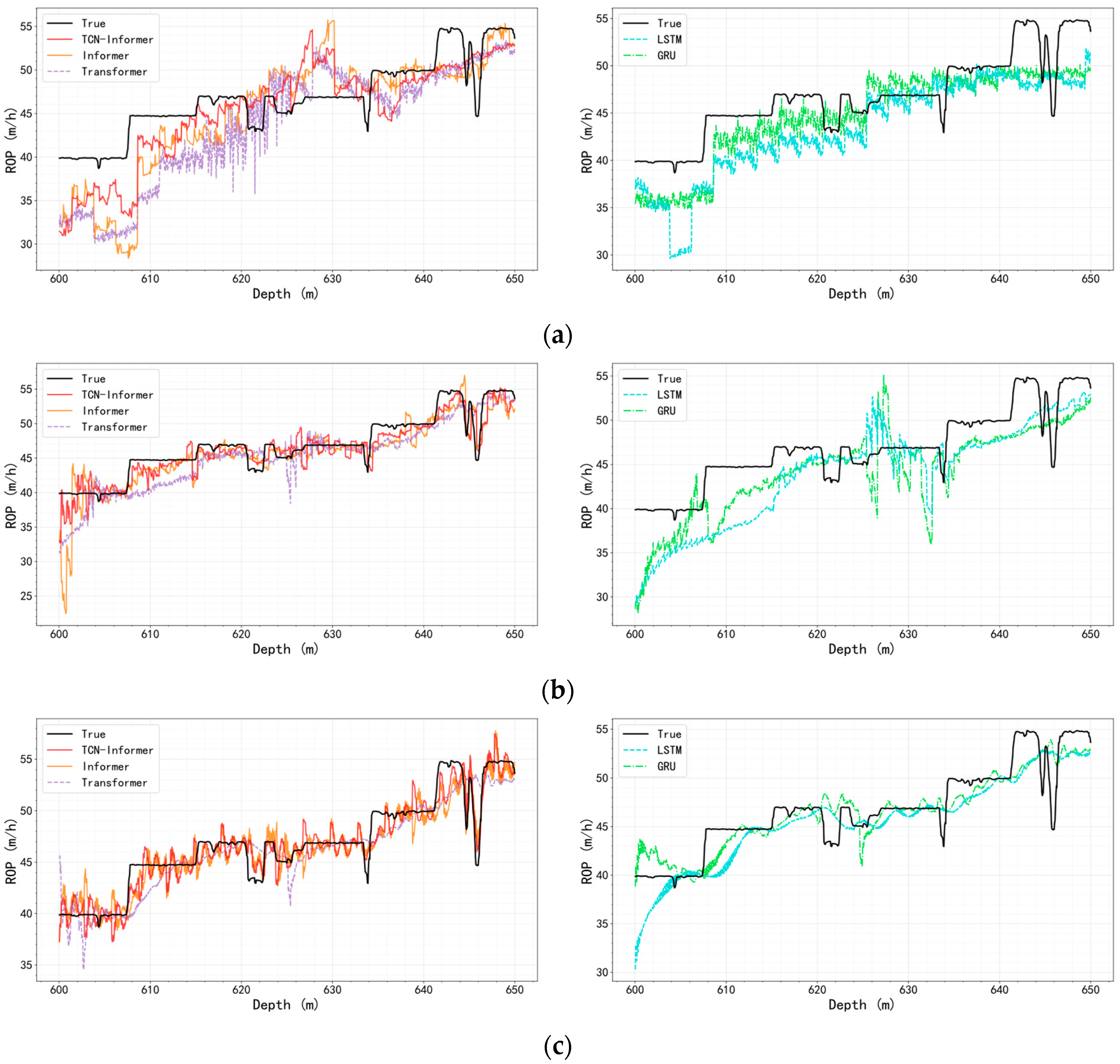
The visualized curves in Figure 10 reinforce these quantitative results. Under varying input and prediction lengths, the TCN–Informer model delivers smaller residuals, shorter phase lags, and smoother long-horizon extrapolations compared to other models. Under the short-sequence setting, LSTM and GRU—limited by effective memory—often show phase lag and amplitude compression. Transformer and Informer capture part of the long-range dependencies but are more sensitive to local high-frequency disturbances and noise, leading to overshoot near turning points. In contrast, TCN–Informer uses causal dilated convolutions to extract short-period components and local inertia, while sparse attention aligns distant key dependencies. This yields more accurate arrival times and amplitudes at abrupt changes.

As input and prediction lengths grow, LSTM and GRU exhibit stronger error accumulation and oscillations. Transformer and Informer frequently show lag and oscillation near abrupt changes. TCN–Informer produces smaller residual fluctuations and phase deviations, smoother long-horizon extrapolation, and stronger trend consistency.

In summary, across different combinations of input and prediction window lengths, TCN–Informer consistently delivers smaller residuals, weaker phase lag, and more stable multi-length prediction performance. These results highlight a complementary mechanism: the TCN branch provides a clean short-term prior, and the Informer, via sparse attention, efficiently aligns distant critical evidence.

5. Conclusions

5.1. Summary

This study addresses the challenges of low prediction accuracy, high computational complexity, and poor adaptability to complex well conditions in traditional models for ROP prediction in drilling engineering. The core issue lies in the inability of single models to simultaneously capture local short-term fluctuations and long-range dependencies in drilling data, which is characterized by strong nonstationarity, sparsity of key events, and susceptibility to noise interference.

To solve this problem, a hybrid TCN–Informer model is proposed, which integrates the advantages of TCN and Informer. TCN leverages its causal dilated convolutions and residual connections to effectively extract local features of the drilling sequence. This capability effectively compensates for the single Informer model’s inadequacy in capturing short-term mechanical vibrations and local inertia. Informer leverages its ProbSparse self-attention and generative decoder to reduce the time and space complexity of long-sequence processing. This design addresses the traditional Transformer’s inefficiency in handling long drilling sequences. Additionally, the model optimizes the structure by removing the distilling layer from Informer and WeightNorm from TCN, and adjusts the input embedding method to enhance feature representation.

For data preprocessing, a four-step strategy is adopted: data deduplication, sliding-window quantile outlier detection, isolation forest secondary outlier detection, and KNN resampling to address data quality issues such as repetition, anomalies, and uneven distribution. The experiment uses the USROP dataset, selecting Well #1, Well #2, and Well #3 for validation. Evaluation indicators include MAE, RMSE, and R², with sliding-window training and Bayesian hyperparameter search based on Optuna to optimize model parameters.

Experimental results show that the TCN–Informer model outperforms single models such as Informer, LSTM, GRU, and Transformer under various input and prediction length combinations. For instance, under the short-sequence setting (input 12, predict 3), the proposed model reduces MAE and RMSE by 24.3% and 18.5%, respectively, and increases R² by 2.1% compared to the Informer model. In contrast, under the long-sequence setting (input 192, predict 48), it achieves reductions of 11.8% in MAE and 8.4% in RMSE, while demonstrating a more substantial improvement in R², which increases by 5.7%. The model demonstrates better responsiveness to sudden ROP changes and more stable prediction in steady-state intervals, verifying its effectiveness and adaptability in ROP prediction.

5.2. Limitations

Despite the satisfactory performance of the TCN–Informer model in ROP prediction, this study still has certain limitations. Firstly, the data preprocessing stage focuses on outlier removal and resampling, but lacks in-depth processing of missing data. In actual drilling operations, sensor failures or data transmission interruptions often lead to large-scale missing data, which may affect the model’s input reliability and prediction stability, and this aspect needs further improvement. Secondly, the model is validated only on the USROP dataset, and the drilling conditions (such as formation type, drilling equipment, and operating parameters) in this dataset are relatively limited. There is a lack of verification on datasets from different regions, complex formation environments (e.g., high-temperature and high-pressure formations), or special drilling technologies (e.g., horizontal well drilling), which may restrict the generalization ability of the model in more diverse practical scenarios. Thirdly, the model’s hyperparameter optimization relies on Optuna’s Bayesian search with a limited number of searches and fixed patience, which may fail to fully explore the optimal hyperparameter combination, and there is room for improvement in optimization efficiency and accuracy.

5.3. Future Directions

Future research can be carried out in the following directions. First, the model’s validation scope should be expanded. This involves collecting drilling data from different regions, formation types, and technologies to build a more diverse and comprehensive dataset. Subsequently, the model’s adaptability and stability need to be verified in complex and variable practical environments, ultimately enhancing its generalization ability. Precisely, the integration of multi-source data can be implemented by standardizing and coordinating multi-source inputs through unified modalities and ontologies, or by employing feature-level fusion with temporal alignment or multi-view learning to integrate these data sources. This approach enables robust cross-modal learning while preserving modality-specific information. Second, the hyperparameter optimization strategy should be improved. For instance, multi-objective optimization algorithms (e.g., NSGA-II) could be incorporated to balance model accuracy and computational efficiency. Alternatively, adaptive hyperparameter adjustment mechanisms could be adopted to reduce reliance on manual tuning and enhance the optimization outcome. Third, the integration of domain knowledge (e.g., drilling mechanics principles, formation lithology characteristics) into the model design should be explored, such as adding domain-guided attention mechanisms or feature engineering modules, to further improve the model’s physical interpretability and prediction accuracy for complex drilling scenarios. Specifically, for the aforementioned research directions in integrating physical models, one can impose physical information constraints or loss terms based on drilling mechanics, encompassing relationships between drilling pressure, torque, mechanical drilling rate, and drill-bit–rock interactions. Alternatively, hybrid models can be developed by combining data-driven predictors with reduced-order or differentiable physical simulators to regularize training and ensure physically consistent outputs.