Wavelet-Guided Zero-Reference Diffusion for Unsupervised Low-Light Image Enhancement

Abstract

Low-light image enhancement (LLIE) remains a challenging task due to the scarcity of paired training data and the complex signal-dependent noise inherent in low-light scenes. To address these issues, this paper proposes a fully unsupervised framework named Wavelet-Guided Zero-Reference Diffusion (WZD) for natural low-light image restoration. WZD leverages an ImageNet-pre-trained diffusion prior and a multi-scale representation of the Discrete Wavelet Transform (DWT) to restore natural illumination from a single dark image. Specifically, the input low-light image is first processed by a Practical Exposure Corrector (PEC) to provide an initial robust luminance baseline. It is then converted from the RGB to the YCbCr color space. The Y channels of the input image and the current diffusion estimate are decomposed into four orthogonal sub-bands—LL, LH, HL, and HH—and fused via learnable, step-wise weights while preserving structural integrity. An exposure control loss and a detail consistency loss are jointly employed to suppress over/under-exposure and preserve high-frequency details. Unlike recent approaches that rely on complex supervised training or lack physical guidance, our method integrates wavelet guidance with a zero-reference learning framework, incorporates the PEC module as a physical prior, and achieves significant improvements in detail preservation and noise suppression without requiring paired training data. Comprehensive experiments on the LOL-v1, LOL-v2, and LSRW datasets demonstrate that WZD achieves a superior or competitive performance, surpassing all referenced unsupervised methods. Ablation studies confirm the critical roles of the PEC prior, YCbCr conversion, wavelet-guided fusion, and the joint loss function. WZD also enhances the performance of downstream tasks, verifying its practical value.

1. Introduction

Low-light imaging remains an enduring challenge in computer vision because of the combined effects of limited camera gain and severe read-out noise, which jointly produce images with low brightness, low contrast, color casts, and indefinite noise [1]. These degradations not only compromise human visual perception but also severely degrade the accuracy of downstream tasks such as object detection, segmentation, and tracking. Traditional solutions [2,3,4,5] based on histogram equalization, Retinex theory, or physics-inspired priors often require labor-intensive hyperparameter tuning and struggle to model real noise distributions and complex illumination variations. Although recent supervised deep learning methods [6,7,8] have achieved remarkable progress by leveraging large-scale paired datasets, the acquisition of well-aligned low/normal-light images is prohibitively expensive, and synthetic degradation models fail to faithfully reproduce the intricate characteristics of real low-light scenes, leading to unsatisfactory generalization across devices and environments. Consequently, developing LLIE algorithms that operate without paired data and that can accurately model realistic noise and illumination remains both scientifically compelling and industrially significant.

Diffusion models [9], widely recognized for their robust capability in modeling high-dimensional data distributions, have exhibited a superior performance in tasks such as image generation, super-resolution imaging, and image restoration. The step-by-step denoising process of a diffusion model naturally separates image content from noise, which directly meets the dual need of low light enhancement: noise removal and brightness recovery. However, current diffusion-based enhancement methods [1,10,11] still rely on paired data or supervised fine-tuning, leaving the unsupervised potential of DMs largely unexplored.

To summarize, the main contributions of this work are as follows: (1) In this paper, we present Wavelet-Guided Zero-Reference Diffusion (WZD), an unsupervised low-light image enhancement framework that operates on a single dark image. WZD synergizes an ImageNet-pre-trained diffusion prior with the multi-scale representation of the Discrete Wavelet Transform (DWT) to progressively restore natural illumination while preserving structural fidelity. (2) We introduce a preprocessing stage where the input image undergoes Practical Exposure Correction (PEC) to establish a robust initial luminance baseline, followed by conversion from the RGB to the YCbCr color space. Only the Y channels of both the input image and the intermediate diffusion estimate are decomposed via DWT into four orthogonal sub-bands (LL, LH, HL, HH), which are adaptively fused using learnable weights at each reverse diffusion step. (3) We design a joint loss function combining an exposure control loss to suppress over- and under-exposure and a novel detail consistency loss to preserve high-frequency structural information. (4) Extensive experiments on the LOL-v1, LOL-v2, and LSRW datasets demonstrate that WZD outperforms all compared unsupervised methods, while subjective evaluations confirm its superior visual quality with minimal artifacts.

The remainder of this paper is organized as follows: Section 2 reviews related work on LLIE and diffusion-based image restoration. Section 3 details the proposed WZD framework, including the diffusion model, DWT, PEC, and wavelet-guided sampling. Section 4 presents the experimental results, including qualitative/quantitative comparisons, ablation studies, and object detection evaluations. Section 5 concludes the work and discusses future directions.

2. Related Work

2.1. Low-Light Image Enhancement

Low-light image enhancement remains a classical yet challenging task in computer vision. A large number of studies have been devoted to translating low-illumination images into visually pleasing normal-light counterparts.

Early efforts focused on histogram equalization and its variants. Ooi and Mat Isa [2] proposed a quadrant dynamic histogram equalization (QDHE) method. It divides a histogram into four sub-histograms, clips the sub-histograms based on the mean of intensity occurrence, then assigns a new dynamic range to each sub-histogram and performs equalization. Fu et al. [5] proposed a fusion-based enhancing method. It derives three inputs, which are the original illumination, the illumination with brightness, and the illumination with contrast enhanced by CLAHE. After designing and normalizing the weights, it obtains the adjusted illumination through multi-scale pyramid fusion. Subsequently, methods based on Retinex decompose an observed image into illumination and reflectance components, reconstructing the enhanced result by estimating an illumination map under carefully designed priors. K. Ng and Wang [4] proposed a total variation Retinex model, based on the assumptions of the spatial smoothness of illumination and the piecewise continuity of reflection. It constructs an energy functional and solves it using alternating minimization combined with the split Bregman method. Nevertheless, these approaches rely on manually designed statistical rules and lack adaptive learning, semantic perception, and targeted noise suppression capabilities in complex scenes. Their dependence on manual parameter fine-tuning also constrains their generalization ability.

With the widespread adoption of deep learning, learning-based methods have achieved remarkable progress in low-light image enhancement. Benefiting from large-scale synthetic and real paired datasets, numerous works learn direct mappings from low-light to normal-light images via end-to-end regression or multi-stage strategies. Guo and Hu [12] proposed a method based on the YCbCr luminance–chrominance space, which uses the Illumination Adjustment Network (IAN), the Adaptive Noise Suppression Network (ANSN), the Noise Fusion Module (NFM), and the Color Adaption Network (CAN) for processing to alleviate noise and color cast in low-light images. Wang et al. [13] introduced an Illumination-Aware Gamma Correction network (IAGC). It adaptively learns global and local correction factors through the Global Gamma Correction Module (GGCM) and Local Gamma Correction Module (LGCM), respectively. It also introduces the Completely Modeling Vision Transformer (COMO-ViT) block to model the dependencies of all pixels in an image. Several studies fuse Retinex principles into neural architectures to learn simultaneous image decomposition and illumination correction. Wei et al. [14] designed the Retinex-Net deep learning framework composed of Decom-Net, which decomposes images into reflectance and illumination; Enhance-Net, which adjusts illumination; and a reflectance denoising operation. Cai et al. [15] proposed a Transformer-based method called Retinexformer, which constructs a one-stage Retinex-based framework (ORF) and designs an Illumination-Guided Transformer (IGT) with Illumination-Guided Multi-head Self-Attention (IG-MSA) as the corruption restorer. Yan et al. [16] proposed a new Horizontal/Vertical Intensity (HVI) color space, which can reduce the distance of red coordinates via polarized HS maps to eliminate red noise, and compress low-light regions with a learnable intensity function to remove black noise. It designed a dual-branch Color and Intensity Decoupling Network (CIDNet) that models color and intensity information separately in the HVI space. Although these methods yield impressive PSNR and SSIM scores [17], their performance heavily relies on the quality and quantity of paired data.

To alleviate the paired data bottleneck, unsupervised approaches exploit unpaired data or self-supervised signals. Jiang et al. [18] proposed a method called EnlightenGAN without paired supervision. Based on a one-path generative adversarial network, it introduces a global–local discriminator, self-regularized self-feature preserving loss, and self-regularized attention mechanism. Guo et al. [19] proposed a zero-reference deep curve estimation method named Zero-DCE. It trains a lightweight DCE-Net to predict pixel-wise high-order curves, guided by non-reference losses including spatial consistency, exposure control, color constancy, and illumination smoothness, thereby eliminating the need for either paired or unpaired training data. Liu et al. [20] proposed a method based on Retinex theory called RUAS. It designs a reference-free cooperative bilevel learning strategy. It automatically discovers prior architectures for illumination estimation and noise removal from a compact search space, and finally constructs a lightweight, computationally efficient and high-performance enhancement network. Ma et al. [6] introduced a Self-Calibrated Illumination (SCI) learning framework. It constructs a cascaded illumination learning process with weight sharing, designs a self-calibrated module, and defines an unsupervised training loss to improve the model’s adaptability to complex scenarios. These approaches operate without the limitation of paired data. However, the enhanced images often suffer from artifacts, detail blurring, and color shifts, and their restoration capability is limited under extremely low-light conditions.

2.2. Diffusion Models for Image Restoration

Diffusion models have been extensively investigated for image restoration tasks such as rain and haze removal [21,22], underwater image restoration [23,24], and low-light image enhancement [25,26]. Most existing approaches train diffusion models on large-scale paired datasets, using degraded images as explicit guidance during the diffusion process to perform restoration. Jiang et al. [27] proposed a wavelet-based conditional diffusion model named DiffLL that leverages the advantages of wavelet transforms to improve efficiency and incorporates a high-frequency recovery module for detail reconstruction. Wang et al. [28] integrated a diffusion model called ExposureDiffusion with a physics-based exposure model, achieving low light enhancement in the raw image space through progressive optimization and adaptive residual layers. Shang et al. [10] proposed a Multi-Domain Multi-Scale (MDMS) diffusion model. This model solves the problem that existing diffusion methods ignore frequency domain features and that single-resolution sampling causes checkerboard artifacts by using a multi-domain learning module with spatial–frequency fusion, a multi-scale sampling strategy, and Bright Channel Prior (BCP). Yin et al. [29] proposed a Structure-guided Diffusion Transformer-based Low-light image enhancement (SDTL) framework. It compresses features via wavelet transform, designs a Structure Enhancement Module (SEM) that uses structural priors and adopts an adaptive fusion strategy, and proposes a Structure-guided Attention Block (SAB) to make the network focus on texture-rich tokens.

Beyond paired data regimes, several methods restore degraded images without any paired samples by exploiting priors from physical models or pre-trained diffusion models. Jiang et al. [30] introduced LightenDiffusion, which combines Retinex theory with diffusion models and introduces a Content Transfer Decomposition Network (CTDN) operating in the latent space along with a self-constrained consistency loss, attaining notable performance gains in unsupervised low light enhancement. He et al. [31] proposed a zero-reference diffusion model named Zero-LED. This model achieves unsupervised training through bidirectional constraints between an initial optimization network and the diffusion model, reduces computational consumption by integrating wavelet transform, and introduces a text and frequency domain-based Appearance Reconstruction Module (ARM). Lv et al. [32] proposed a method named FourierDiff, embedding Fourier priors into a pre-trained diffusion model. By leveraging Fourier prior-guided diffusion sampling and spatial–frequency alternating optimization, it achieves natural brightness and a clear structure jointly without requiring paired training data or degradation assumptions. Wang et al. [33] proposed a zero-reference framework, which designs a physical quadruple prior based on the Kubelka–Munk light transfer theory, serving as a bridge between low-light and normal-light images; is trained only with normal-light images; builds a prior-to-image map by combining a pre-trained generative diffusion model; and introduces a bypass decoder to handle detail distortion. He et al. [34] proposed a method which combines the wavelet domain and Fourier frequency domain to construct rich prior information. It is embedded into a pre-trained diffusion model. It also introduces multimodal text embedding and simplifies a denoising module. However, the inference speed of this method is slow, and it will take a long time to process large-scale image data.

3. Method

3.1. Diffusion Model

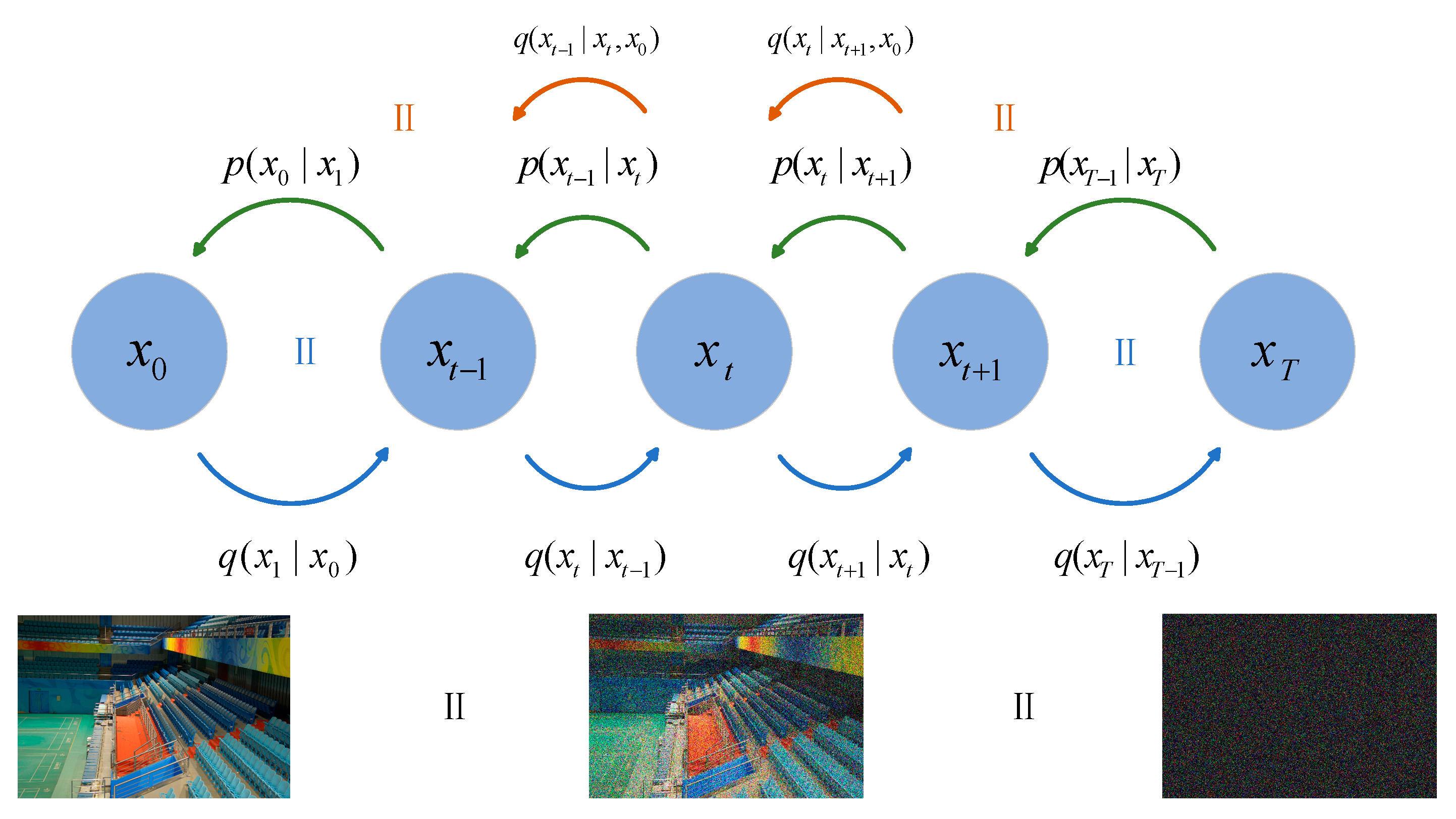
Denoising Diffusion Probabilistic Models (DDPMs) are a class of deep generative models built upon a Markovian diffusion process, which are widely recognized for their training stability and high synthesis fidelity. The pipeline comprises two phases: forward diffusion and reverse denoising (see Figure 1).

3.1.1. Forward Diffusion

Let $x_0~q(x_0)$ be a real image. Given a monotonically increasing noise schedule ${\left\{{\beta }_t\right\}}_{t=1}^T$ with $0<{\beta }_1<\cdots <{\beta }_T<1$, each step $t$ adds Gaussian noise to $x_{t-1}$ as follows:

$$q(x_t\mid x_{t-1})=\mathcal{N}(x_t;\sqrt{1-{\beta }_t}{x}_{t-1},{\beta }_{t}I)$$

(1)

Using the re-parameterization trick, the latent variable at any step $t$ can be sampled in closed form as follows:

$$x_t=\sqrt{{\overline{\alpha }}_t}{x}_0+\sqrt{1-{\overline{\alpha }}_t}ϵ,\hspace{1em}ϵ~\mathcal{N}(0,I)$$

(2)

where ${\alpha }_t=1-{\beta }_t$ and ${\overline{\alpha }}_t={\displaystyle \prod _{i=1}^t{\alpha }_i}$. For sufficiently large $T$, $x_T$ is approximately standard Gaussian.

3.1.2. Reverse Denoising

To recover $x_0$ from $x_T$, we learn the reverse transition $p_{\theta }(x_{t-1}\mid x_t)$. DDPM parameterizes it as a Gaussian as follows:

$$p_{\theta }(x_{t-1}\mid x_t)=\mathcal{N}(x_{t-1};{\mu }_{\theta }(x_t,t),{\sigma }_t^{2}I)$$

(3)

with variance ${\sigma }_t^2$ commonly fixed to ${\beta }_t$ or ${\tilde{\beta }}_t$ to reduce parameters. Since $q(x_{t-1}\mid x_t,x_0)$ is tractable, the network only needs to predict the injected noise ${ϵ}_{\theta }(x_t,t)$, yielding

$${\mu }_{\theta }(x_t,t)={\displaystyle \frac{1}{\sqrt{{\alpha }_t}}}\left(x_t-{\displaystyle \frac{{\beta }_t}{\sqrt{1-{\overline{\alpha }}_t}}}{ϵ}_{\theta }(x_t,t)\right)$$

(4)

where ${ϵ}_{\theta }(x_t,t)$ is the estimated noise predicted by a deep neural network. According to Ho et al. [9], the model randomly samples a noise $ϵ~\mathcal{N}(0,I)$, then optimizes the network parameters $\theta$ with the following objective function:

$${\mathcal{L}}_{\mathrm{simple}}={\mathbb{E}}_{x_0,ϵ,t}\left[\Vert ϵ-{ϵ}_{\theta }(x_t,t){\Vert }^2\right]$$

(5)

At inference, starting from $x_T~\mathcal{N}(0,I)$, we iteratively apply

$$x_{t-1}={\displaystyle \frac{1}{\sqrt{{\alpha }_t}}}\left(x_t-{\displaystyle \frac{{\beta }_t}{\sqrt{1-{\overline{\alpha }}_t}}}{ϵ}_{\theta }(x_t,t)\right)+{\sigma }_{t}z,\hspace{1em}z~\mathcal{N}(0,I)$$

(6)

until we obtain a high-quality sample $x_0$ after $T$ steps.

3.2. The Discrete Wavelet Transform

The Discrete Wavelet Transform (DWT) is grounded in multiresolution analysis and employs a complementary pair of finite impulse response (FIR) low-pass and high-pass filters. It performs separable convolution on image rows and columns of an image, followed by dyadic downsampling, yielding four mutually orthogonal sub-bands: LL, which encodes the low-frequency approximation and global luminance; LH, which captures vertical high-frequency components corresponding to horizontal edges; HL, which represents horizontal high-frequency components associated with vertical edges; and HH, which retains diagonal high-frequency information pertinent to corners and fine-scale details. The Inverse DWT (IDWT) enables lossless reconstruction of the original image by reversing the upsampling process and using corresponding synthesis filters. Owing to the regularity, vanishing moments, and directional selectivity of the wavelet bases, the resulting wavelet coefficients exhibit a sparse, energy-concentrated distribution: low-frequency coefficients dominate the signal energy, while high-frequency coefficients sparsely encode local singularities. This characteristic thus provides a powerful prior for the diffusion model to implement progressive denoising and detail recovery.

3.3. Practical Exposure Correction

Practical Exposure Corrector (PEC) [35] is proposed to address the problems of poor generalization in existing data-driven deep networks and time-consuming inference in traditional optimization methods. Its basic mathematical model is defined as follows:

$$\left\{\begin{array}{l}{x}_u=y+ϵ(y),\mathrm{if} y\in \mathbb{U}\hfill \\ x_o=y-ϵ(y),\mathrm{if} y\in \mathbb{O}\hfill \end{array}\right.$$

(7)

where $y$ denotes the input image with abnormal exposure; $x_u$ and $x_o$ represent the corrected results for under- and over-exposed regions. The sets $\mathbb{U}$ and $\mathbb{O}$ represent the under-exposed and over-exposed image domains. $\mathit{ϵ}(y)$ is the exposure-sensitive compensation, which is the core quantity to be dynamically generated by the algorithm.

To generate the exposure-sensitive compensation term $\mathit{ϵ}(y)$, PEC introduces three synergistic modules. To eliminate the need for external training data, PEC devises an exposure adversarial function, defined as

$$f(z)=cz\otimes (1-z)$$

(8)

where $z\in {[0,1]}^{m\times n}$ is the input image with normalized pixel values, $\otimes$ represents the element-wise multiplication, and $c\in [0,1]$ is a coefficient for controlling exposure level.

This function has two key properties: it satisfies the axisymmetric property $f(z)=f(1-z)$, ensuring that symmetric compensation intensities are generated for under-exposed pixels and over-exposed pixels. Meanwhile, the output range of the function is constrained to $[0,0.25c]$, which can avoid pixel overflow caused by over-correction.

The second component is a warm start with compensation, which is proposed to provide an effective initialization, which can be formulated as

$$\left\{\begin{array}{ll}{g}_u(y)=y+f(y),\hfill & \mathrm{if} \mathrm{UC}\hfill \\ g_o(y)=y-f(y),\hfill & \mathrm{if} \mathrm{OC}\hfill \end{array}\right.$$

(9)

where $g_u$ and $g_o$ are the corrected outputs for under-exposure and over-exposure cases.

At this point, the initial value of the exposure-sensitive compensation is $\mathit{ϵ}(y)=f(y)$. This mechanism has the following scene symmetry property: if $c$ is identical on different exposure scenes, it satisfies $g_u(1-y)=1-g_o(y)$, reflecting the reverse correlation between the correction of the two exposure scenarios.

The third component is the segmented shrinkage iterative scheme. This scheme optimizes $\mathit{ϵ}(y)$ through multiple rounds of iteration and ensures the convergence of the algorithm. It consists of multiple shrinkage built-in blocks (denoted as $t$), and each block contains several iteration steps (denoted as $k$). The basic iterative formulas are

$$\left\{\begin{array}{l}{h}_u^k(y):x_u^k=g_u(y)+f(x_u^{k-1})\hfill \\ h_o^k(y):x_o^k=g_o(y)-f(x_o^{k-1})\hfill \end{array}\right.$$

(10)

The iteration starts from the warm start results, i.e., $x_u^0=g_u(y)$ and $x_o^0=g_o(y)$. This scheme has the shrinkage property: as the number of iterations increases, the variation in the compensation gradually decreases and finally converges to the optimal value.

3.4. Wavelet-Guided Zero-Reference Diffusion Sampling

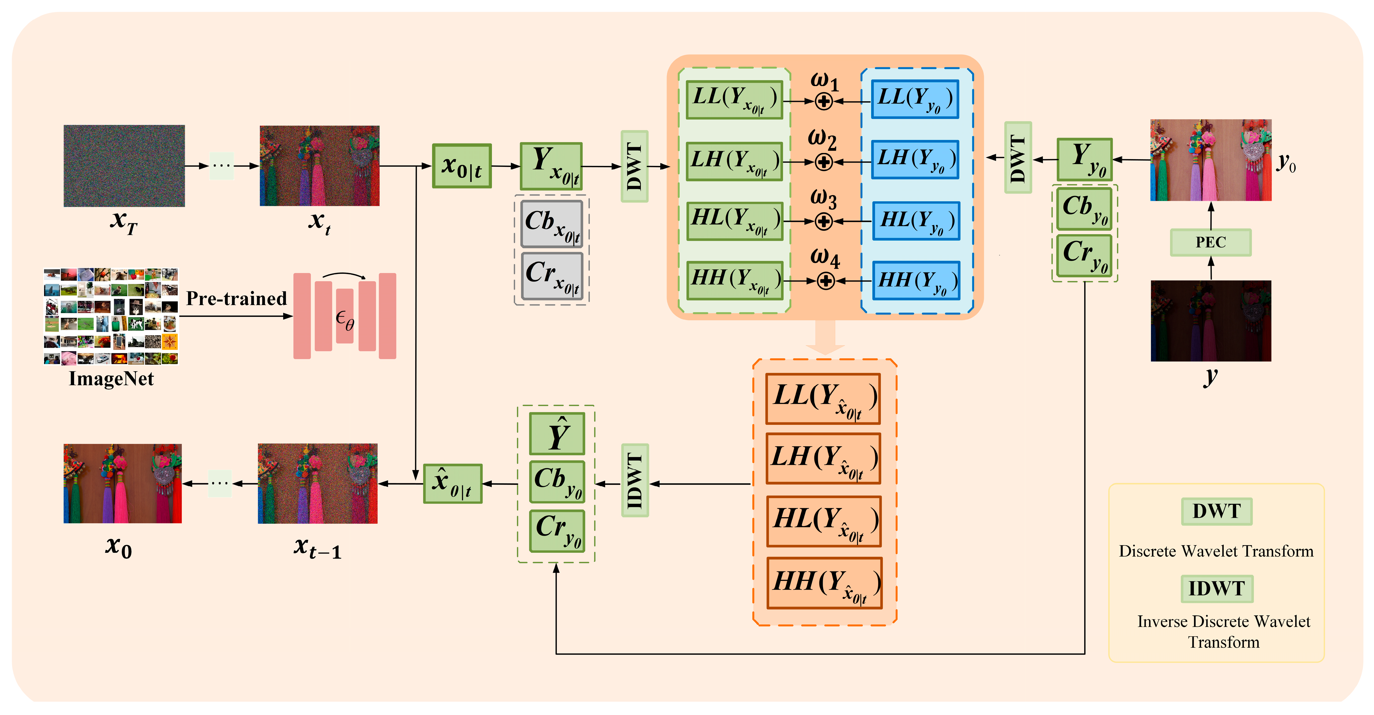
The proposed framework operates in a zero-reference setting: given only a single low-light image $y$, it produces a visually pleasing normal-light image $x_0$ by leveraging a diffusion model pre-trained on a large corpus of natural-light images and wavelet domain information. As illustrated in Figure 2, our method starts from pure Gaussian noise $x_T~\mathcal{N}(0,I)$ and progressively refines it into $x_0$ through the reverse diffusion process.

Specifically, we adopt a 256 × 256 diffusion model [36] pre-trained on ImageNet whose internal priors encapsulate real-world illumination statistics. To prevent the loss of content guidance in dark inputs, we prime the pipeline with PEC using a conservative exposure parameter, thereby providing an initial luminance baseline before diffusion sampling begins. At every denoising step $t$, we first obtain an intermediate estimate $x_{0|t}$ conditioned on $x_t$ using the standard DDPM formulation:

$$x_{0|t}={\displaystyle \frac{1}{\sqrt{{\overline{\alpha }}_t}}}\left(x_t-{ϵ}_{\theta }(x_t,t)\sqrt{1-{\overline{\alpha }}_t}\right)$$

(11)

To achieve color preservation, we convert the input low-light image from the RGB space to the YCbCr space. Here, Y denotes the luminance component, Cb denotes the blue chrominance component, and Cr denotes the red chrominance component. Subsequently, we only perform wavelet decomposition and fusion on the Y channel, while the Cb and Cr channels are temporarily stored.

$$Y_{x_{0|t}},C{b}_{x_{0|t}},C{r}_{x_{0|t}}=RGB2YCbCr(x_{0|t})$$

(12)

$$Y_{y_0},C{b}_{y_0},C{r}_{y_0}=RGB2YCbCr(y_0)$$

(13)

Next, we decompose both $Y_{x_{0|t}}$ and $Y_{y_0}$ via the DWT, yielding four sub-bands for each of the following: $\left\{LL(Y_{x_{0|t}}),\hspace{0.33em}LH(Y_{x_{0|t}}),\hspace{0.33em}HL(Y_{x_{0|t}}),\hspace{0.33em}HH(Y_{x_{0|t}})\right\}$ $\left\{LL(Y_{y_0}),\hspace{0.33em}LH(Y_{y_0}),\hspace{0.33em}HL(Y_{y_0}),\hspace{0.33em}HH(Y_{y_0})\right\}$. To inject natural light priors while preserving low-light structural cues, we perform a learnable sub-band fusion:

$$LL(Y_{{\hat{x}}_{0|t}})=LL(Y_{y_0})+w_{1}LL(Y_{x_{0|t}})$$

(14)

$$LH(Y_{{\hat{x}}_{0|t}})=LH(Y_{y_0})+w_{2}LH(Y_{x_{0|t}})$$

(15)

$$HL(Y_{{\hat{x}}_{0|t}})=HL(Y_{y_0})+w_{3}HL(Y_{x_{0|t}})$$

(16)

$$HH(Y_{{\hat{x}}_{0|t}})=HH(Y_{y_0})+w_{4}HH(Y_{x_{0|t}})$$

(17)

where ${\left\{w_i\right\}}_{i=1}^4$ are learnable scalar weights shared across all pixels. The fused sub-bands are then transformed back to the spatial domain via the IDWT:

$$\hat{Y}=IDWT(LL(Y_{{\hat{x}}_{0|t}}),LH(Y_{{\hat{x}}_{0|t}}),HL(Y_{{\hat{x}}_{0|t}}),HH(Y_{{\hat{x}}_{0|t}}))$$

(18)

We combine the processed luminance component with the original chrominance components and convert them back to the RGB space to obtain ${\hat{x}}_{0|t}$

$${\hat{x}}_{0|t}=YCbCr2RGB(\hat{Y},C{b}_{y_0},C{r}_{y_0})$$

(19)

Finally, we compute the next denoised sample $x_{t-1}$ using the standard reverse diffusion update as follows:

$$p_{\theta }\left(x_{t-1}\mid x_t,{\hat{x}}_{0|t}\right)=\mathcal{N}\left(x_{t-1};{\mu }_t\left(x_t,{\hat{x}}_{0|t}\right),{\sigma }_t^{2}I\right)$$

(20)

Repeating this wavelet-guided refinement at every reverse step yields the final enhanced image $x_0$ with natural illumination characteristics.

Additionally, to compensate for under-exposure and suppress over-exposure, we incorporate an Exposure Control Loss as follows [19]:

$${\mathcal{L}}_{exp}={\displaystyle \frac{1}{M}}{\displaystyle \sum _{k=1}^M|Y_k-E|}$$

(21)

where $M$ denotes the preset number of non-overlapping local regions, $Y_k$ represents the mean intensity within the $k$-th region of the enhanced image, and $E$ represents the brightness level.

To preserve high-frequency details during image enhancement and avoid over-smoothing or artifact introduction, we propose a detail consistency loss function. This loss extracts high-frequency components from both $Y_{y_0}$ and $\hat{Y}$ using the Laplacian operator and constrains their differences.

High-frequency details are extracted using the following Laplacian convolution kernel:

$$K_{lap}=\left[\begin{array}{ccc}0& 1& 0\\ 1& -4& 1\\ 0& 1& 0\end{array}\right]$$

(22)

The detail maps are obtained through the following 2D convolution operations:

$$\begin{array}{l}{D}_{enh}=\mathrm{conv}2\mathrm{d}(\hat{Y},K_{lap})\\ D_{y_0}=\mathrm{conv}2\mathrm{d}(Y_{y_0},K_{lap})\end{array}$$

(23)

The final detail consistency loss function is defined as

$${\mathcal{L}}_{detail}={\displaystyle \frac{1}{N}}{\displaystyle \sum _{i=1}^N\left|D_{enh}^{(i)}-D_{y_0}^{(i)}\right|}$$

(24)

where $N$ denotes the total number of pixels and $|\cdot |$ represents the absolute value operation. We utilize ${\mathcal{L}}_1$ norm to measure detail differences for enhanced robustness against outliers. This loss function effectively preserves edge sharpness and textural details, thereby improving the visual quality of the enhancement results.

By integrating the two aforementioned loss functions, the final loss function is given by

$${\mathcal{L}}_{total}={\mathcal{L}}_{\exp }+{\mathcal{L}}_{detail}$$

(25)

4. Experiments

4.1. Experimental Set-Up

We implement our framework with Pytorch 1.11.0 on a single NVIDIA GeForce RTX 4090 GPU. We set the batch size to 1 and resized all test images to 256 × 256. For the PEC module, we set the exposure control coefficient $c$ = 0.4, the number of shrinkage built-in blocks $t$ = 3, and the iteration steps $k$ = [3, 3, 3]. In the diffusion model, we employ the sampling steps $T$ = 100, set travel_length to 1, and use linear betas of (0.0001, 0.02). We adopt the Adam optimizer [37] with a learning rate of 1 × 10⁻². Additionally, we set the brightness level $E$ to 0.6.

We evaluated our method on the widely used LOL-v1 [14], LOL-v2 [38], and LSRW [39] datasets. Image quality is assessed with the Peak Signal-to-Noise Ratio (PSNR), Structural Similarity Index (SSIM) [17], and Learned Perceptual Image Patch Similarity (LPIPS) [40] metrics. In addition, we introduce two non-reference perceptual metrics Natural Image Quality Evaluator (NIQE) [41] and Blind/Referenceless Image Spatial Quality Evaluator (BRISQUE) [42] to measure the visual quality.

4.2. Qualitative Comparison

To thoroughly evaluate our model, we select several unsupervised low-light image enhancement methods—Zero-DCE [19], EnlightenGAN [18], RUAS [20], SCI [6], the low light enhancement branch of FourierDiff [32] (denoted as FourierDiff_LLIE), and JWFPGD [34]—and conduct evaluations on the supervised LOL-v1, LOL-v2, and LSRW datasets using their officially released implementations. Among the unsupervised low-light image enhancement methods compared in this paper, Zero-DCE [19], EnlightenGAN [18], RUAS [20], and SCI [6] are classic representative methods. Many subsequent related studies take them as baseline methods for performance comparison. In contrast, FourierDiff_LLIE [32] and JWFPGD [34] are advanced methods proposed in the field of low light enhancement during 2024–2025. Specifically, the LSRW dataset contains images captured by Nikon cameras and Huawei smartphones. The LSRW_Nikon dataset consists of 3150 pairs of training images and 20 pairs of test images, while the LSRW_Huawei dataset comprises 2450 pairs of images, with 30 pairs allocated for testing. The results are shown in Figure 3, Figure 4, Figure 5 and Figure 6.

As illustrated in Figure 3, it can be observed that the images processed via Zero-DCE [19] and SCI [6] remain dark overall and are still affected by some noise that impairs image quality. Although the EnlightenGAN-based [18] method outperforms the previous two in restoring image brightness, significant noise is still observed in the enhanced images. There is a certain degree of color distortion relative to the ground truth, and partial blurring occurs at the blue lines within the boxed regions. For images processed using RUAS [20] and FourierDiff-LLIE [32], relatively good overall brightness restoration is achieved. However, noise of varying degrees still exists, and the regions with high brightness in the original images undergo brightness over-enhancement after enhancement, which obscures some details. Although the image processed by the JWFPGD [34] method can effectively restore the normal illumination level, it still exhibits significant deficiencies in detail restoration. Specifically, the object edges in the region of interest show obvious block artifacts. Our approach successfully restores natural illumination while preserving high perceptual quality, exhibiting superior spatial smoothness. In contrast to competing methods, it introduces virtually no visible noise or artifacts.

A visual inspection of Figure 4 reveals that images restored using Zero-DCE [19] and EnlightenGAN [18] exhibit unexpected black artifacts near the light sources of the original images, which impairs the visual effects of the images. Images processed via RUAS [20] and FourierDiff-LLIE [32] both present noise of varying degrees, compromising image quality. Meanwhile, in images restored by RUAS, the light sources in the original images are nearly invisible. In the image restored by FourierDiff-LLIE [32], the edges of the light source in the original image become blurred, resulting in a decrease in contrast with the surrounding environment. The image enhanced through SCI [6] also shows significant noise, which affects image quality. The image processed by the JWFPGD method [34] still exhibits obvious block artifacts, which seriously degrades the image’s visual quality. In contrast to competing approaches, our method not only restores natural illumination and accurate color balance but also preserves the integrity and radiance of the original light sources within the scene.

From the results in Figure 5, qualitative comparisons can be observed between our method and competing approaches on the LSRW_Huawei dataset. The regions of interest are highlighted with red bounding boxes; magnified views of these patches are displayed in the bottom-right corners of the corresponding images. Although the methods based on Zero-DCE [19], EnlightenGAN [18], and RUAS [20] can effectively achieve normal illumination restoration, their overall colors still exhibit significant deviations from the ground truth. Further observation reveals that the methods based on RUAS [20] and SCI [6] suffer from detail loss, specifically manifested in the fact that the cloud edges in the input image are barely visible after processing. In addition, the FourierDiff-LLIE [32] and JWFPGD [34] methods still manifest obvious deficiencies in normal illumination restoration capability, and the overall brightness of the images processed by them still has a significant difference from that of the ground truth. While restoring normal illumination, our proposed method exerts no significant impact on image color and incurs no significant detail loss.

It can be seen from the results in Figure 6, Zero-DCE [19], FourierDiff-LLIE [32], and JWFPGD [34] exhibit obvious deficiencies in normal illumination restoration capability, and the overall brightness of the images processed by them still manifests a significant difference from the ground truth. However, these three methods perform well in preserving the details of the original image. Meanwhile, the images processed by the EnlightenGAN [18] and RUAS [20] methods show a significant deviation in overall color from the ground truth. Furthermore, the image processed by RUAS [20] also suffers from severe detail loss, specifically manifested in the fact that the brick gaps in the region of interest are barely visible. In addition, the image processed by the SCI [6] method has an over-exposure issue compared with the ground truth, and the detail loss is also severe. By contrast, the image processed by our proposed method can effectively restore normal illumination while well preserving the details in the image.

4.3. Quantitative Comparison

We quantitatively evaluate our method with several unsupervised low-light image enhancement methods, including PSNR, SSIM [17], LPIPS [40], NIQE [41], and BRISQUE [42]. The results are shown in

Table 1. Quantitative comparison of our method and other unsupervised methods on LOL-v1. The best results are highlighted in bold. The second-best results are underlined.

Methods	PSNR ↑ *	SSIM ↑ *	LPIPS ↓ *	NIQE ↓ *	BRISQUE ↓ *
Zero-DCE [19]	14.86	0.666	0.224	7.373	28.365
EnlightenGAN [18]	17.48	0.717	0.229	4.649	15.303
RUAS [20]	16.40	0.702	0.215	6.741	15.392
SCI [6]	14.78	0.619	0.208	7.449	27.454
FourierDiff_LLIE [32]	18.05	0.727	0.193	6.090	20.777
JWFPGD [34]	19.39	0.802	0.190	5.549	23.141
Ours	19.18	0.821	0.191	5.296	10.479

* The upward arrow (↑) indicates that a higher value is better, and the downward arrow (↓) indicates that a lower value is better.

,

Table 2. Quantitative comparison of our method and other unsupervised methods on LOL-v2. The best results are highlighted in bold. The second-best results are underlined.

Methods	PSNR ↑ *	SSIM ↑ *	LPIPS ↓ *	NIQE ↓ *	BRISQUE ↓ *
Zero-DCE [19]	18.06	0.680	0.210	7.513	36.742
EnlightenGAN [18]	18.64	0.729	0.232	4.918	24.032
RUAS [20]	15.33	0.672	0.241	6.742	21.190
SCI [6]	17.30	0.632	0.187	7.581	35.241
FourierDiff_LLIE [32]	16.86	0.701	0.212	6.260	30.413
JWFPGD [34]	18.01	0.772	0.206	5.553	28.837
Ours	19.46	0.823	0.166	5.577	19.272

* The upward arrow (↑) indicates that a higher value is better, and the downward arrow (↓) indicates that a lower value is better.

,

Table 3. Quantitative comparison of our method and other unsupervised methods on LSRW_Huawei. The best results are highlighted in bold. The second-best results are underlined.

Methods	PSNR ↑ *	SSIM ↑ *	LPIPS ↓ *	NIQE ↓ *	BRISQUE ↓ *
Zero-DCE [19]	16.41	0.482	0.237	3.691	31.166
EnlightenGAN [18]	17.85	0.521	0.259	3.563	23.955
RUAS [20]	12.53	0.351	0.274	4.358	28.889
SCI [6]	15.70	0.445	0.225	3.893	29.837
FourierDiff_LLIE [32]	16.87	0.520	0.237	3.604	30.261
JWFPGD [34]	17.54	0.559	0.233	4.129	38.504
Ours	19.12	0.600	0.226	4.439	27.455

* The upward arrow (↑) indicates that a higher value is better, and the downward arrow (↓) indicates that a lower value is better.

and

Table 4. Quantitative comparison of our method and other unsupervised methods on LSRW_Nikon. The best results are highlighted in bold. The second-best results are underlined.

Methods	PSNR ↑ *	SSIM ↑ *	LPIPS ↓ *	NIQE ↓ *	BRISQUE ↓ *
Zero-DCE [19]	15.05	0.421	0.175	3.778	25.423
EnlightenGAN [18]	15.92	0.429	0.179	3.593	22.433
RUAS [20]	13.76	0.376	0.189	4.111	37.309
SCI [6]	14.56	0.414	0.151	3.956	33.792
FourierDiff_LLIE [32]	13.79	0.397	0.162	4.036	35.112
JWFPGD [34]	13.62	0.403	0.166	4.350	34.668
Ours	16.61	0.487	0.141	4.136	35.514

* The upward arrow (↑) indicates that a higher value is better, and the downward arrow (↓) indicates that a lower value is better.

. To intuitively demonstrate the performance differences between our method and other comparative methods, we plotted radar charts based on the data in Table 1, Table 2, Table 3 and Table 4, as shown in Figure 7. To address the issues of inconsistent numerical scales and conflicting variation directions among different metrics, we performed normalization on the data in the tables. Finally, we define that in the radar charts, the closer the value is to 1, the better the metric performs.

PSNR [17] is a classic metric for measuring the pixel-level errors between enhanced images and reference images. In the test results on the LOLv2, LSRW_Huawei, and LSRW_Nikon datasets, the PSNR values of our method exceed that of all comparative methods. In the testing experiments on the LOLv1 dataset, our proposed method achieves a sub-optimal performance in terms of the PSNR metric. This indicates that our method performs optimally in pixel-level error control. The enhanced images have the smallest pixel difference from ideal reference images and the highest pixel-level restoration accuracy.

SSIM [17] is a metric that, from the perspective of human visual perception, measures the similarity between enhanced images and reference images in three dimensions—brightness, contrast, and structure. Similarly, our method outperforms other reference methods in the test results on all datasets, highlighting its advantages in structure preservation and visual consistency. It demonstrates that our method can not only enhance the brightness of low-light images but also preserve structural features, making the enhanced images visually closer to real-world scenarios.

By simulating the perceptual mechanism of the human visual system, LPIPS [40] quantifies the difference between enhanced images and reference images. A lower value indicates greater similarity between the two images at the perceptual level. In the testing experiments on the LOLv1 and LSRW_Huawei datasets, our proposed method achieves a sub-optimal performance in terms of the LPIPS metric; while in those on the LOLv2 and LSRW_Nikon datasets, it achieves an optimal performance. This result shows that the images enhanced by our method are more natural, rarely exhibiting a sense of incongruity such as color distortion or brightness contrast discontinuity, thus achieving excellent perceptual quality.

NIQE [41] evaluates image quality by analyzing the degree of deviation between the statistical characteristics of an image and those of natural images. In the testing experiments on all datasets, our proposed method exhibits advantageous performance in terms of the NIQE metric. This implies that in application scenarios without ideal reference images, the results of our method can still maintain high naturalness, and their statistical characteristics are closer to those of real natural images.

BRISQUE [42] focuses on the spatial domain quality of images and evaluates quality by extracting the natural scene statistical features of images. In the testing experiments on the LOLv1 and LOLv2 datasets, our proposed method achieves an optimal performance in terms of the BRISQUE metric; in those on the LSRW_Huawei and LSRW_Nikon datasets, the method exhibits an advantageous performance in the same metric. This result indicates that the results obtained by our method exhibit excellent spatial domain quality. The enhanced images have high definition and low noise residue.

Based on a comprehensive analysis of all metrics, our method demonstrates a comprehensive and balanced low-light image enhancement performance.

4.4. Ablation Study

We conduct ablation studies to evaluate (i) the necessity of priming dark inputs with Practical Exposure Correction (PEC) [35] prior to diffusion sampling; (ii) the effectiveness of converting images from the RGB space to the YCbCr space for subsequent processing; (iii) the effectiveness of decomposing the images via DWT and subsequently fusing the corresponding sub-bands with learnable weights; (iv) the effectiveness of the two introduced loss functions (i.e., ${\mathcal{L}}_{exp}$ and ${\mathcal{L}}_{detail}$). Specifically, we compare the full pipeline of our proposed method against five ablated variants: (i) w/o PEC, which omits the conservative exposure pre-correction, (ii) w/o YCbCr, which processes images directly in the RGB space instead of converting them to the YCbCr space first; (iii) w/o DWT, which replaces wavelet-based fusion with a naïve pixel-wise weighted summation; (iv) w/o ${\mathcal{L}}_{detail}$, which uses only the ${\mathcal{L}}_{exp}$ loss function without ${\mathcal{L}}_{detail}$; (v) w/o ${\mathcal{L}}_{exp}$, which uses only the ${\mathcal{L}}_{detail}$ loss function without ${\mathcal{L}}_{exp}$. All configurations are evaluated on four datasets, including LOL-v1, LOL-v2, LSRW-Huawei, and LSRW-Nikon. The results are shown in Figure 8 and

Table 5. Ablation studies of our method on LOL-v1. The best results are highlighted in bold. The second-best results are underlined.

Methods	PSNR ↑ *	SSIM ↑ *	LPIPS ↓ *	NIQE ↓ *	BRISQUE ↓ *
w/o PEC	14.10	0.632	0.400	6.679	40.191
w/o YCbCr	19.31	0.820	0.194	5.109	10.750
w/o DWT	17.00	0.713	0.207	6.366	22.783
$\mathrm{w}/\mathrm{o} {\mathcal{L}}_{detail}$	19.06	0.821	0.177	5.542	13.296
$\mathrm{w}/\mathrm{o} {\mathcal{L}}_{exp}$	13.41	0.684	0.193	5.514	13.336
Ours	19.18	0.821	0.191	5.296	10.480

* The upward arrow (↑) indicates that a higher value is better, and the downward arrow (↓) indicates that a lower value is better.

,

Table 6. Ablation studies of our method on LOL-v2. The best results are highlighted in bold. The second-best results are underlined.

Methods	PSNR ↑ *	SSIM ↑ *	LPIPS ↓ *	NIQE ↓ *	BRISQUE ↓ *
w/o PEC	15.39	0.599	0.352	6.660	36.427
w/o YCbCr	19.60	0.820	0.192	5.495	19.223
w/o DWT	14.93	0.673	0.196	6.604	32.756
$\mathrm{w}/\mathrm{o} {\mathcal{L}}_{detail}$	19.23	0.820	0.154	5.770	21.637
$\mathrm{w}/\mathrm{o} {\mathcal{L}}_{exp}$	17.15	0.717	0.169	5.788	23.536
Ours	19.46	0.823	0.166	5.577	19.272

* The upward arrow (↑) indicates that a higher value is better, and the downward arrow (↓) indicates that a lower value is better.

,

Table 7. Ablation studies of our method on LSRW_Huawei. The best results are highlighted in bold. The second-best results are underlined.

Methods	PSNR ↑ *	SSIM ↑ *	LPIPS ↓ *	NIQE ↓ *	BRISQUE ↓ *
w/o PEC	14.05	0.500	0.408	7.520	71.583
w/o YCbCr	19.17	0.594	0.220	4.450	27.752
w/o DWT	14.45	0.526	0.238	3.487	29.734
$\mathrm{w}/\mathrm{o} {\mathcal{L}}_{detail}$	18.81	0.586	0.213	4.284	27.036
$\mathrm{w}/\mathrm{o} {\mathcal{L}}_{exp}$	15.72	0.525	0.219	4.412	29.641
Ours	19.12	0.600	0.226	4.439	27.455

* The upward arrow (↑) indicates that a higher value is better, and the downward arrow (↓) indicates that a lower value is better.

and

Table 8. Ablation studies of our method on LSRW_Nikon. The best results are highlighted in bold. The second-best results are underlined.

Methods	PSNR ↑ *	SSIM ↑ *	LPIPS ↓ *	NIQE ↓ *	BRISQUE ↓ *
w/o PEC	11.80	0.386	0.234	5.666	46.767
w/o YCbCr	16.47	0.481	0.137	4.032	34.270
w/o DWT	12.44	0.416	0.208	4.055	44.737
$\mathrm{w}/\mathrm{o} {\mathcal{L}}_{detail}$	16.41	0.479	0.152	4.239	35.959
$\mathrm{w}/\mathrm{o} {\mathcal{L}}_{exp}$	16.18	0.470	0.134	4.128	35.118
Ours	16.61	0.487	0.141	4.136	35.514

* The upward arrow (↑) indicates that a higher value is better, and the downward arrow (↓) indicates that a lower value is better.

.

The results of the ablation studies demonstrate that each core component in our proposed method contributes significantly to the final performance. A detailed analysis is as follows: (1) Removing the PEC component leads to a significant performance degradation, which confirms the necessity of performing robust exposure pre-correction on low-light input images prior to diffusion sampling. (2) The contribution of YCbCr space conversion is relatively moderate. After removing this component, the model’s performance on some perceptual metrics is similar to that of the full pipeline, but the full pipeline still exhibits superior or comparable performance stability across most key metrics. (3) Removing the wavelet decomposition and DWT sub-band weighted fusion module results in significant degradation in PSNR and SSIM across all datasets. This proves the superiority of multi-sub-band fusion in the frequency domain for preserving image details and structural information. (4) The ablation results of the loss functions show that the exposure loss function ${\mathcal{L}}_{exp}$ is crucial for regulating image exposure and contrast, and serves as the core to maintain high PSNR and SSIM metrics; the detail loss function ${\mathcal{L}}_{detail}$ helps further improve image structural similarity. When the two functions work synergistically, the model achieves an optimal balance between objective metrics and perceptual quality.

In conclusion, the ablation studies systematically verify the effectiveness of each core design choice in the proposed method.

4.5. Effect on Object Detection

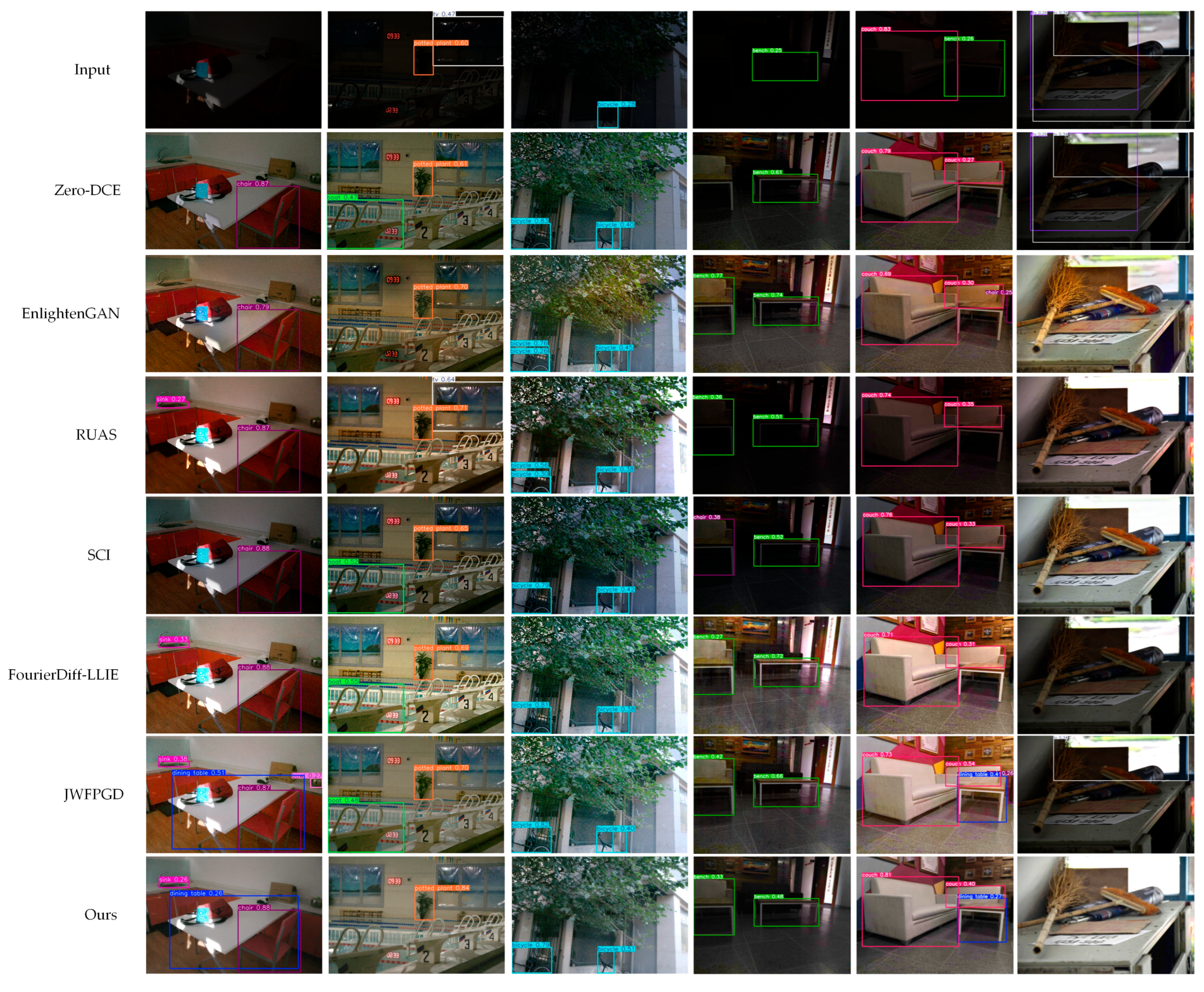
We conducted experiments on downstream tasks such as object detection to demonstrate the practical value of our method. Specifically, we employed the pre-trained YOLO11 model provided officially by Ultralytics on the COCO dataset. The results are shown in Figure 9. The first row presents the object detection results on the original low-light images, while the remaining rows show the object detection results on images processed by Zero-DCE [19], EnlightenGAN [18], RUAS [20], SCI [6], FourierDiff-LLIE [32], JWFPGD [34], and our proposed method.

The results indicate that although YOLO11 has achieved significant improvements in object detection capability compared with its previous versions, it still suffers from issues such as missed detections and false detections in low-light environments. After processing with low light enhancement algorithms, the overall brightness of the images is significantly improved, and the detection accuracy of YOLO11 also increases accordingly. By comparing these low light enhancement methods, it can be seen that our proposed method not only performs excellently in its low light enhancement performance but also performs prominently in assisting YOLO11 in improving detection accuracy.

In fact, deep learning-based object detectors such as YOLO operate on a core mechanism of extracting low-level features and high-level features from input images in a stepwise manner and accomplish object detection through multi-scale feature fusion and anchor box matching. However, the inherent defects of low-light images directly interfere with this process, which manifests specifically in three aspects. Insufficient brightness causes low-level features of objects to be obscured by noise and low-illumination conditions, making it difficult for object detectors to capture an adequate number of discriminative features and thus leading to missed detections. Meanwhile, the pervasive signal-dependent noise in low-light images may be misidentified as “spurious features” or directly mask the real features of objects, resulting in false detections or missed detections. Additionally, the contrast imbalance and color distortion often associated with low-light images lead to significant discrepancies between the brightness distribution and color features of objects, and the normal-light images used for YOLO’s pre-training. This makes it difficult for the object detector to effectively match the pre-trained category features and accurately distinguish the object–background boundaries. In contrast, the method proposed in this paper can enhance the brightness of images while achieving color fidelity and detail restoration, addressing the aforementioned interference of low-light images on detection and improving object detection accuracy effectively.

5. Conclusions

This paper introduced the Wavelet-Guided Zero-Reference Diffusion (WZD) framework, a fully unsupervised approach for low-light image enhancement that effectively addresses the challenges of paired data scarcity and complex noise in real-world low-light conditions. The framework establishes a systematic pipeline: it first primes the dark input using a Practical Exposure Corrector (PEC) to establish a robust initial luminance baseline, then converts the image to the YCbCr color space. All subsequent enhancements are performed exclusively on the Y channel, thereby preserving color fidelity. The core of WZD integrates a pre-trained diffusion model prior with the multi-scale analysis capability of the Discrete Wavelet Transform (DWT) at each reverse denoising step, decomposing the Y channels of the input image and the intermediate estimate into orthogonal sub-bands for learnable fusion. Furthermore, a novel combination of an exposure control loss and a detail consistency loss is introduced to suppress over/under-exposure while preserving critical high-frequency texture.

Extensive experiments on three benchmark datasets—LOL-v1, LOL-v2, and LSRW—demonstrate that WZD attains a highly competitive performance across a comprehensive set of five full-reference and no-reference metrics (PSNR, SSIM, LPIPS, NIQE, BRISQUE), surpassing all compared unsupervised baselines. Both qualitative and quantitative results confirm its superior ability to restore natural illumination with minimal artifacts and color distortion. Ablation studies verify the indispensability of each core component and their specific order: the PEC prior for initial luminance correction, the YCbCr color space conversion for color preservation, the DWT-based fusion for detail recovery, and the joint loss function for balanced perceptual quality. The practical value of WZD is further validated through its positive impact on the accuracy of downstream tasks such as object detection.

Future work will focus on developing more efficient sampling strategies to facilitate the deployment of this high-performance low light enhancement algorithm on resource-constrained, latency-critical platforms such as unmanned aerial vehicles and autonomous vehicles.

References

1. Yi, X.; Xu, H.; Zhang, H.; Tang, L.; Ma, J. Diff-Retinex: Rethinking Low-Light Image Enhancement with A Generative Diffusion Model. In Proceedings of the 2023 IEEE/CVF International Conference on Computer Vision (ICCV), Paris, France, 2–6 October 2023; pp. 12268–12277. [Google Scholar]
2. Ooi, C.H.; Mat Isa, N.A. Quadrants Dynamic Histogram Equalization for Contrast Enhancement. IEEE Trans. Consum. Electron. 2010, 56, 2552–2559. [Google Scholar] [CrossRef]
3. Jobson, D.J.; Rahman, Z.; Woodell, G.A. A Multiscale Retinex for Bridging the Gap between Color Images and the Human Observation of Scenes. IEEE Trans. Image Process. 1997, 6, 965–976. [Google Scholar] [CrossRef] [PubMed]
4. Ng, M.K.; Wang, W. A Total Variation Model for Retinex. SIAM J. Imaging Sci. 2011, 4, 345–365. [Google Scholar] [CrossRef]
5. Fu, X.; Zeng, D.; Huang, Y.; Liao, Y.; Ding, X.; Paisley, J. A Fusion-Based Enhancing Method for Weakly Illuminated Images. Signal Process. 2016, 129, 82–96. [Google Scholar] [CrossRef]
6. Ma, L.; Ma, T.; Liu, R.; Fan, X.; Luo, Z. Toward Fast, Flexible, and Robust Low-Light Image Enhancement. In Proceedings of the 2022 IEEE/CVF Conference on Computer Vision and Pattern Recognition (CVPR), New Orleans, LA, USA, 19–24 June 2022; pp. 5627–5636. [Google Scholar]
7. Wu, W.; Weng, J.; Zhang, P.; Wang, X.; Yang, W.; Jiang, J. URetinex-Net: Retinex-Based Deep Unfolding Network for Low-Light Image Enhancement. In Proceedings of the 2022 IEEE/CVF Conference on Computer Vision and Pattern Recognition (CVPR), New Orleans, LA, USA, 19–24 June 2022; pp. 5891–5900. [Google Scholar]
8. Liu, R.; Ma, L.; Ma, T.; Fan, X.; Luo, Z. Learning With Nested Scene Modeling and Cooperative Architecture Search for Low-Light Vision. IEEE Trans. Pattern Anal. Mach. Intell. 2023, 45, 5953–5969. [Google Scholar] [CrossRef]
9. Ho, J.; Jain, A.; Abbeel, P. Denoising Diffusion Probabilistic Models. arXiv 2020, arXiv:2006.11239. [Google Scholar] [CrossRef]
10. Shang, K.; Shao, M.; Wang, C.; Cheng, Y.; Wang, S. Multi-Domain Multi-Scale Diffusion Model for Low-Light Image Enhancement. In Proceedings of the Thirty-Eighth AAAI Conference on Artificial Intelligence and Thirty-Sixth Conference on Innovative Applications of Artificial Intelligence and Fourteenth Symposium on Educational Advances in Artificial Intelligence, Vancouver, BC, Canada, 20–27 February 2024; Volume 38, pp. 4722–4730. [Google Scholar]
11. Feng, Y.; Hou, S.; Lin, H.; Zhu, Y.; Wu, P.; Dong, W.; Sun, J.; Yan, Q.; Zhang, Y. DiffLight: Integrating Content and Detail for Low-Light Image Enhancement. In Proceedings of the 2024 IEEE/CVF Conference on Computer Vision and Pattern Recognition Workshops (CVPRW), Seattle, WA, USA, 17–18 June 2024; pp. 6143–6152. [Google Scholar]
12. Guo, X.; Hu, Q. Low-Light Image Enhancement via Breaking Down the Darkness. Int. J. Comput. Vis. 2023, 131, 48–66. [Google Scholar] [CrossRef]
13. Wang, Y.; Liu, Z.; Liu, J.; Xu, S.; Liu, S. Low-Light Image Enhancement with Illumination-Aware Gamma Correction and Complete Image Modelling Network. In Proceedings of the 2023 IEEE/CVF International Conference on Computer Vision (ICCV), Paris, France, 2–6 October 2023; pp. 13082–13091. [Google Scholar]
14. Wei, C.; Wang, W.; Yang, W.; Liu, J. Deep Retinex Decomposition for Low-Light Enhancement. arXiv 2018, arXiv:1808.04560. [Google Scholar] [CrossRef]
15. Cai, Y.; Bian, H.; Lin, J.; Wang, H.; Timofte, R.; Zhang, Y. Retinexformer: One-Stage Retinex-Based Transformer for Low-Light Image Enhancement. arXiv 2023, arXiv:2303.06705. [Google Scholar]
16. Yan, Q.; Feng, Y.; Zhang, C.; Pang, G.; Shi, K.; Wu, P.; Dong, W.; Sun, J.; Zhang, Y. HVI: A New Color Space for Low-Light Image Enhancement. arXiv 2025, arXiv:2502.20272. [Google Scholar] [CrossRef]
17. Wang, Z.; Bovik, A.C.; Sheikh, H.R.; Simoncelli, E.P. Image Quality Assessment: From Error Visibility to Structural Similarity. IEEE Trans. Image Process. 2004, 13, 600–612. [Google Scholar] [CrossRef] [PubMed]
18. Jiang, Y.; Gong, X.; Liu, D.; Cheng, Y.; Fang, C.; Shen, X.; Yang, J.; Zhou, P.; Wang, Z. EnlightenGAN: Deep Light Enhancement Without Paired Supervision. IEEE Trans. Image Process. 2021, 30, 2340–2349. [Google Scholar] [CrossRef] [PubMed]
19. Guo, C.; Li, C.; Guo, J.; Loy, C.C.; Hou, J.; Kwong, S.; Cong, R. Zero-Reference Deep Curve Estimation for Low-Light Image Enhancement. In Proceedings of the 2020 IEEE/CVF Conference on Computer Vision and Pattern Recognition (CVPR), Online, 14–19 June 2020; pp. 1777–1786. [Google Scholar]
20. Liu, R.; Ma, L.; Zhang, J.; Fan, X.; Luo, Z. Retinex-Inspired Unrolling with Cooperative Prior Architecture Search for Low-Light Image Enhancement. In Proceedings of the 2021 IEEE/CVF Conference on Computer Vision and Pattern Recognition (CVPR), Online, 20–25 June 2021; pp. 10556–10565. [Google Scholar]
21. Wen, Y.; Gao, T.; Chen, T. Unpaired Photo-Realistic Image Deraining with Energy-Informed Diffusion Model. In Proceedings of the 32nd ACM International Conference on Multimedia, Melbourne, Australia, 28 October 2024; pp. 360–369. [Google Scholar]
22. Wang, J.; Wu, S.; Yuan, Z.; Tong, Q.; Xu, K. Frequency Compensated Diffusion Model for Real-Scene Dehazing. Neural Netw. 2024, 175, 106281. [Google Scholar] [CrossRef] [PubMed]
23. Liu, S.; Li, K.; Ding, Y.; Qi, Q. Underwater Image Enhancement by Diffusion Model with Customized CLIP-Classifier. arXiv 2024, arXiv:2405.16214. [Google Scholar] [CrossRef]
24. Tang, Y.; Iwaguchi, T.; Kawasaki, H. Underwater Image Enhancement by Transformer-Based Diffusion Model with Non-Uniform Sampling for Skip Strategy. arXiv 2023, arXiv:2309.03445. [Google Scholar]
25. Xue, M.; He, J.; Wang, W.; Zhou, M. Low-Light Image Enhancement via CLIP-Fourier Guided Wavelet Diffusion. arXiv 2024, arXiv:2401.03788. [Google Scholar] [CrossRef]
26. Zhou, H.; Dong, W.; Liu, X.; Zhang, Y.; Zhai, G.; Chen, J. Low-Light Image Enhancement via Generative Perceptual Priors. arXiv 2024, arXiv:2412.20916. [Google Scholar] [CrossRef]
27. Jiang, H.; Luo, A.; Han, S.; Fan, H.; Liu, S. Low-Light Image Enhancement with Wavelet-Based Diffusion Models. arXiv 2023, arXiv:2306.00306. [Google Scholar] [CrossRef]
28. Wang, Y.; Yu, Y.; Yang, W.; Guo, L.; Chau, L.-P.; Kot, A.C.; Wen, B. ExposureDiffusion: Learning to Expose for Low-Light Image Enhancement. arXiv 2023, arXiv:2307.07710. [Google Scholar]
29. Yin, X.; Yu, Z.; Jiang, L.; Gao, X.; Sun, X.; Liu, Z.; Yang, X. Structure-Guided Diffusion Transformer for Low-Light Image Enhancement. arXiv 2025, arXiv:2504.15054. [Google Scholar] [CrossRef]
30. Jiang, H.; Luo, A.; Liu, X.; Han, S.; Liu, S. LightenDiffusion: Unsupervised Low-Light Image Enhancement with Latent-Retinex Diffusion Models. arXiv 2024, arXiv:2407.08939. [Google Scholar]
31. He, J.; Xue, M.; Ning, A.; Song, C. Zero-LED: Zero-Reference Lighting Estimation Diffusion Model for Low-Light Image Enhancement. arXiv 2024, arXiv:2403.02879. [Google Scholar]
32. Lv, X.; Zhang, S.; Wang, C.; Zheng, Y.; Zhong, B.; Li, C.; Nie, L. Fourier Priors-Guided Diffusion for Zero-Shot Joint Low-Light Enhancement and Deblurring. In Proceedings of the 2024 IEEE/CVF Conference on Computer Vision and Pattern Recognition (CVPR), Seattle, WA, USA, 17–21 June 2024; pp. 25378–25388. [Google Scholar]
33. Wang, W.; Yang, H.; Fu, J.; Liu, J. Zero-Reference Low-Light Enhancement via Physical Quadruple Priors. arXiv 2024, arXiv:2403.12933. [Google Scholar]
34. He, J.; Palaiahnakote, S.; Ning, A.; Xue, M. Zero-Shot Low-Light Image Enhancement via Joint Frequency Domain Priors Guided Diffusion. IEEE Signal Process. Lett. 2025, 32, 1091–1095. [Google Scholar] [CrossRef]
35. Ma, L.; Ma, T.; Xue, X.; Fan, X.; Luo, Z.; Liu, R. Practical Exposure Correction: Great Truths Are Always Simple. arXiv 2022, arXiv:2212.14245. [Google Scholar] [CrossRef]
36. Dhariwal, P.; Nichol, A. Diffusion Models Beat GANs on Image Synthesis. arXiv 2021, arXiv:2105.05233. [Google Scholar] [CrossRef]
37. Kingma, D.P.; Ba, J. Adam: A Method for Stochastic Optimization. arXiv 2017, arXiv:1412.6980. [Google Scholar] [CrossRef]
38. Yang, W.; Wang, W.; Huang, H.; Wang, S.; Liu, J. Sparse Gradient Regularized Deep Retinex Network for Robust Low-Light Image Enhancement. IEEE Trans. Image Process. 2021, 30, 2072–2086. [Google Scholar] [CrossRef] [PubMed]
39. Hai, J.; Xuan, Z.; Yang, R.; Hao, Y.; Zou, F.; Lin, F.; Han, S. R2RNet: Low-Light Image Enhancement via Real-Low to Real-Normal Network. J. Vis. Commun. Image Represent. 2023, 90, 103712. [Google Scholar] [CrossRef]
40. Zhang, R.; Isola, P.; Efros, A.A.; Shechtman, E.; Wang, O. The Unreasonable Effectiveness of Deep Features as a Perceptual Metric. In Proceedings of the 2018 IEEE/CVF Conference on Computer Vision and Pattern Recognition, Salt Lake City, UT, USA, 18–22 June 2018; pp. 586–595. [Google Scholar]
41. Mittal, A.; Soundararajan, R.; Bovik, A.C. Making a “Completely Blind” Image Quality Analyzer. IEEE Signal Process. Lett. 2013, 20, 209–212. [Google Scholar] [CrossRef]
42. Mittal, A.; Moorthy, A.K.; Bovik, A.C. No-Reference Image Quality Assessment in the Spatial Domain. IEEE Trans. Image Process. 2012, 21, 4695–4708. [Google Scholar] [CrossRef]
Figure 1. The complete forward diffusion and reverse denoising pipeline. x 0 denotes the original normal-light image; x t denotes the noisy image at diffusion step t; q ( x t | x t 1 ) is the forward diffusion distribution; p ( x t 1 | x t ) is the learned reverse denoising distribution; and q ( x t 1 | x t , x 0 ) is the theoretically true inverse denoising distribution.
Electronics 14 04460 g001
Figure 2. The architecture of our proposed method. The framework takes a single low-light image y as input: first, it performs conservative exposure pre-correction via PEC, then converts the image from RGB to YCbCr space; the reverse diffusion process starts from pure Gaussian noise x T , generating an intermediate estimate x 0 | t at each denoising step t via standard DDPM; next, the Y channels of both y 0 and x 0 | t are decomposed into LL, LH, HL, HH sub-bands by DWT, fused with learnable weights, and transformed back to the spatial domain via IDWT; the processed Y channel is combined with stored Cb/Cr channels and converted to RGB space to obtain x ^ 0 | t ; this process is iterated for each reverse step to output the final enhanced image.
Electronics 14 04460 g002
Figure 3. Qualitative comparisons between our method and competing approaches on the LOL-v1 dataset. Regions of interest are highlighted with red bounding boxes; magnified views of these patches are displayed in the bottom-right corners of the corresponding images.
Electronics 14 04460 g003
Figure 4. Qualitative comparisons between our method and competing approaches on the LOL-v2 dataset. Regions of interest are highlighted with red bounding boxes; magnified views of these patches are displayed in the bottom-right corners of the corresponding images. Note that the Chinese characters present in the background are part of the original scene from the dataset and are not relevant to the algorithmic evaluation.
Electronics 14 04460 g004
Figure 5. Qualitative comparisons between our method and competing approaches on the LSRW_Huawei dataset. Regions of interest are highlighted with red bounding boxes; magnified views of these patches are displayed in the bottom-right corners of the corresponding images. Note that the Chinese characters present in the background are part of the original scene from the dataset and are not relevant to the algorithmic evaluation.
Electronics 14 04460 g005
Figure 6. Qualitative comparisons between our method and competing approaches on the LSRW_Nikon dataset. Regions of interest are highlighted with red bounding boxes; magnified views of these patches are displayed in the bottom-right corners of the corresponding images.
Electronics 14 04460 g006
Figure 7. Radar charts plotted based on the data in Table 1, Table 2, Table 3 and Table 4. To address the issues of inconsistent numerical scales and conflicting variation directions among different metrics, we perform normalization on the data in the tables. Finally, we consider that in the radar charts, the closer the value is to 1, the better the metric performs.
Electronics 14 04460 g007
Figure 8. Ablation studies of our method on LOL-v1, LOL-v2, LSRW_Huawei, and LSRW_Nikon. Note that the Chinese characters present in the background are part of the original scene from the dataset and are not relevant to the algorithmic evaluation.
Electronics 14 04460 g008
Figure 9. The results of object detection. We compare the object detection results obtained by performing object detection on images processed by all compared unsupervised low light enhancement methods, with those obtained by applying our proposed method to images and then conducting object detection.
Electronics 14 04460 g009