Article

A Methodology for Payload Parameter Sensitivity Analysis of Lightweight Electric Vehicle State Prediction

1
School of Mechatronic Engineering and Automation, Shanghai University, Shanghai 200072, China
2
Shanghai Civil Aviation Electromechanical Systems Co., Ltd., Shanghai 200241, China
*
Author to whom correspondence should be addressed.
Electronics 2025, 14(22), 4372; https://doi.org/10.3390/electronics14224372
Submission received: 17 September 2025 / Revised: 5 November 2025 / Accepted: 6 November 2025 / Published: 8 November 2025

Abstract

The Light Electric Vehicle (LEV) possesses the advantages of energy efficiency, environmental friendliness, and excellent control in traffic. Nevertheless, a decrease in vehicle mass and size directly affects the active safety system control and state estimation system of LEVs. This paper presents a novel and efficient analysis technique for evaluating the sensitivity of payload parameter variations on the response and state estimation of the LEV system. Firstly, a dynamic model of the LEV is established, taking into account the payload parameters. Next, the accuracy of the payload parameter trajectory sensitivity is calculated using a combination of the perturbation analysis method and the second-order central difference method. An unscented Kalman filter is specifically developed to estimate various vehicle states, including the sideslip angle, longitudinal velocity, and roll angle. The significance of payload parameters on observation accuracy when payload parameters vary during basic state estimation is assessed. The simulation results obtained using Matlab/Simulink-Carsim® 2019 demonstrate the ability of the method to effectively depict the correlation between the payload parameters and the system state estimation. Quantitatively, the sideslip angle is most sensitive to the payload mass (average sensitivity: 2.15 × 10⁻²), while the longitudinal velocity is predominantly affected by the payload’s longitudinal position. By integrating perturbation analysis with the central difference method, this approach provides a novel and efficient framework for LEV sensitivity analysis, and it is valuable for the design and estimation of the LEV controller.

1. Introduction

With the advancement of clean energy and electronic technology, the active safety control system in lightweight electric vehicles (LEVs) has also been progressing and developing in recent years. Examples of this include the direct yaw control system (DYC) [1,2,3], active front steering system (AFS) [4], anti-lock braking systems (ABSs) [5,6], active suspension system (ASS) [7], and electric power steering system (EPS) [8]. LEVs can also capture the driving, steering, and braking signals of the vehicle in real time, which expands the information collection range of traditional vehicles and enables direct monitoring of vehicle critical condition parameters. Precise estimation of vehicle state information is a crucial component of the active safety control system. Alterations in the load will impact the vehicle’s center of gravity, thus influencing the vehicle’s assessment of its own state and its active safety control system. Notably, the installation of a wireless charging system can also modify the vehicle’s center of gravity, and other types of electric vehicles such as fuel cell electric vehicles also exhibit load variability and parameter uncertainty akin to LEVs—for example, hydrogen consumption alters curb mass and the yaw moment of inertia about the z-axis and redistributes axle vertical loads, and energy-management strategies impose torque constraints [9,10,11]. When examining the dynamic performance of lightweight electric vehicles, it is crucial to thoroughly analyze the dynamic changes in vehicle payload characteristics and their influence on model development. Hence, it is imperative to choose a suitable analytic technique in order to validate the precision and dependability of the model. Vehicle payload sensitivity analysis is considered an effective method for quantifying and analyzing the impact of vehicle parameters on its system dynamic response.
Several researchers have undertaken studies on the examination of vehicle sensitivity analysis. Krishna [12] performed a sensitivity analysis using conditional variance and developed a control algorithm for an Anti-lock Braking System (ABS) based on sliding mode control. The study focused on investigating the impact of tire parameters in the “magic formula” on the performance of the ABS. Huang [13] designed a dynamic control model to examine how changes in payload characteristics affect vehicle dynamic control. The model allows for the observation of differences in vehicle inertia and geometry parameters resulting from changes in payload values. Corno [14] developed a control-oriented electro-hydraulic brake actuator model for racing motorcycles, the parameters in the braking model were identified by the gray box method and a parameter sensitivity analysis of the experimental results was carried out.
As evident from the preceding discussion, numerous research findings are employed in vehicle sensitivity analysis [15,16,17,18,19]. Vehicle sensitivity analysis is used in state estimation to assess the effectiveness of load factors. In addition, many scholars have also discussed the estimation of inertial parameters that affect the control of system dynamics. In lightweight electric vehicles, inertial characteristics are of utmost importance and have been extensively analyzed by numerous experts. A methodology for assessing the performance of hybrid electric bus vehicles is developed by integrating the Extended Kalman Filter (EKF) and Recursive Least Squares (RLS) techniques [15]. The observer described by Hong [16] is a type of unscented Kalman filter known as a dual unscented Kalman filter (DUKF). By locally examining the inertial parameters and states of the nonlinear vehicle model, it is confirmed that the approach is successful and resilient. The study [17] introduced a constrained Dual Kalman Filter (DKF) that utilizes probability density function (pdf) truncation to estimate various states. The study [18] proposed a UKF algorithm combined with the Huber method to realize the state parameter estimation of distributed electric vehicles. The study [19] proposed a new state estimation method to estimate vehicle parameters such as vehicle roll angle, which combines the dual Kalman filter with sensitivity analysis based on variance methods. Although neural networks and deep learning have been used in state estimation, their reliance on large amounts of training data, the existence of black-box model problems, and limited generalization capabilities have limited their application in light electric vehicles (LEVs), which have extremely high safety requirements [20,21,22]. On the other hand, the performance of traditional parameter estimation methods, such as sliding mode observers, relies heavily on the precise tuning of key parameters such as the sliding mode gain [23]. This process is complex and has a direct impact on estimation accuracy and system stability. In the automotive field, especially in parameter estimation, the Kalman filter algorithm offers strong recursiveness, good robustness, and excellent filtering effects. Therefore, it is often the choice of many researchers in systems with high precision requirements.
This paper presents a methodology for conducting a quantitative investigation of the sensitivity of vehicle payload characteristics to the system response and state estimation of distributed drive electric vehicles. This method is specially designed for lightweight electric vehicles, and the sensitivity analysis is carried out by combining the disturbance analysis method and the finite difference method. The UKF approach is utilized for state estimation, while the sensitivity analysis method suggested in this research is employed to solve and analyze the predicted state quantities. The subsequent sections of this document are outlined below. Section 2 presents the estimation model for the nonlinear dynamic system of the vehicle, including the nonlinear model of the vehicle with loaded payload, the nonlinear model of the tire, and the models of the wheels and motors. Section 3 presents the sensitivity analysis technique. Section 4 presents the methodology for building the Unscented Kalman Filter (UKF) estimator. Section 5 provides the simulation outcomes, whereas Section 6 summarizes the conclusions.

2. Load-Oriented Vehicle Dynamics Model

2.1. Vehicle Dynamics Model with Load Parameter Variations

Figure 1 depicts the schematic diagram of the distributed drive electric vehicle dynamics model, encompassing longitudinal, lateral, yaw, and roll motions. The assumptions for the nonlinear vehicle model are as follows [24,25,26]: It is presumed that the left and right front wheels have the same angle, and the influence of steering and transmission mechanisms is disregarded. When examining the total weight of the vehicle, only the weight of the parts supported by the suspension is taken into account, while the weight of the parts not supported by the suspension is disregarded. The movement of the vehicle’s axis caused by rolling, rolling over, and pitching motions is not taken into consideration. These assumptions are reasonable under the studied sinusoidal steering conditions, which makes the model more concise and facilitates highlighting the main effects of payload parameters. However, future work needs to relax these assumptions to improve model fidelity.
The vehicle dynamics equations derived according to D’Alembert’s principle [18,19] are as follows:
m n ( V ˙ x V y r z ) = i , j = 1 2 F x i j F w F f
a x = 1 m i , j = 1 2 F x i j F w F f
i , j = 1 2 F x i j = F x f l cos δ f l F x f l sin δ f l + F x f r cos δ f r F x f r sin δ f r + F x r l + F x r r
F w = 1 2 C d ρ A f V x 2
F f = μ m n g
m n ( V ˙ y + V x r z ) = i , j = 1 2 F y i j
a y = 1 m i , j = 1 2 F y i j
i , j = 1 2 F y i j = F y r l + F y r r + F y f l cos δ f l + F y f r cos δ f r + F y f l sin δ f l + F y r l sin δ f r
I z 0 r ˙ z I x z 0 r ˙ x = l f 0 ( F y f l + F y f r ) l r 0 ( F y r l + F y r r ) + b l 0 ( F x f r + F x r r ) b r 0 ( F x f l + F x r l )
I x 0 r ˙ x I x z 0 r ˙ z = m s g h r sin φ + m s a y h r K φ φ β φ φ ˙
β = arctan ( V y V x )
where Vx and Vy are the longitudinal and lateral velocity at the CG of the vehicle, respectively, and mn is the total mass of the vehicle. rz is the yaw rate at the CG of the vehicle; Fxij and Fyij are the longitudinal and lateral forces of the vehicle’s tires i and j, respectively, where i = f, r; j = l, r; Fw and Ff are the vehicle’s air resistance and the ground tire’s rolling resistance, respectively; Cd is the air resistance coefficient; and ρ is the air density. μ is road surface adhesion coefficient; fl and fr are the front wheel’s left and right wheel angles; ax and ay are the vehicle’s longitudinal and lateral accelerations; Izz is the vehicle’s yaw moment of inertia; and Mz is the vehicle’s yaw moment.
When additional loads are defined, the coordinate vector of the center of gravity changes to:
r n = x n , y n , z n
The change in the coordinate vector of the center of gravity is:
r = x p , y p , z p
When additional loads are added to the vehicle, the total vehicle mass changes to:
m n = m e + m p
The velocity change at the new center of gravity and its differential form after the change in the position of the center of gravity is:
V p = V + r × r n V ˙ = V ˙ p r ˙ × r n
The Euler equations for the rotational motion of the vehicle body are obtained as:
I r ˙ + r ˜ I r = M
During the vehicle motion process, the following definitions are made for the overall rotational inertia and the product of inertia:
I = I x x I x y I x z I x y I y y I y z I x z I y z I z z =   I x 0 + m ( y n 2 + ( z n + h ) 2 ) x n × y n × m n x n × ( z n + h ) × m n x n × y n × m n I y 0 + m n ( y n 2 + ( z n + h ) 2 ) y n × ( z n + h ) × m n x n × ( z n + h ) × m n y n × ( z n + h ) × m n I z 0 + m n ( x n 2 + y n 2 )
The new coordinates of the center of gravity are determined by applying the principle of levers, assuming that the height of the vehicle’s center of gravity remains constant:
m n r n = m e 0 + m p r
r n = m p m n r
The yaw moment of inertia after loading is calculated using the parallel axis theorem:
I z z = I z z o + m n r n 2 2
Since the load mp is a point load, the relationship between the mass after loading and the coordinates of the center of gravity is as follows:
m n r n 2 2 = m p r 2 2 m n r n 2 2
I z z = I z z o + m p r 2 2 m n r n 2 2
Therefore, the calculation of the yaw moment of inertia for the distributed drive electric vehicle is as follows:
I z z = I z z o + m p 1 m p m e + m p r 2 2 = I z z o + m p 1 m p m e + m p x p 2 + y p 2
At the same time, consider the changes in the center of gravity brought by the variable load. In the equation, the parameters of the tire model are calculated as follows:
l f = l f 0 x n ,   l r = l r 0 + x n ,   b l = b l 0 y n , b r = b r 0 + y n ,   l f + l r = L ,   b l + b r = B ,   h n = h r + z n
Among them, lf0 and lr0 are the horizontal distances from the CG of the vehicle to the front and rear axles when not loaded. lf and lr are the horizontal distances from the CG of the vehicle to the front and rear axles after loading; bl0 and br0 are the horizontal distances from the CG of the vehicle to the left and right wheels when the electric vehicle is not loaded. bl and br are the horizontal distance from the CG of the vehicle to the left and right wheels after loading. L is the horizontal distance between the front and rear axles of the vehicle; B is the horizontal distance between the vehicle’s left and right wheels.

2.2. Nonlinear Tire Model

In this paper, the nonlinear Pacejka tire model [20] is selected. The specific formula is as follows:
Y ( x ) = y ( x ) + S v , x = X + S h y = D sin ( C arctan ( B x E ( B x arctan B x ) ) )
In the above formula, Y represents the lateral force Fy and longitudinal force Fx of the tire, X represents the tire lateral angle α or the longitudinal slip rate s, and Sv and Sh represent the vertical drift and horizontal drift of the curve, respectively. The tire model parameters B, C, D, and E are stiffness factor, curve shape factor, peak factor, and curve curvature factor, respectively. Parameter information in the Pacejka model is shown in Table 1.
Given that dynamic loads arising from vehicle movement are unavoidable, they consequently influence the acceleration of the vehicle and ultimately effect the vertical load. The vertical load on the wheel can be defined as follows:
F z f l = m n l f + l r b l + b r l r g b r h b r a x l r h a y , F z f r = m n l f + l r b l + b r l r g b l h b l a x + l r h a y , F z r l = m n l f + l r b l + b r l f g b r + h b r a x l f h a y , F z r r = m n l f + l r b l + b r l f g b l + h b l a x + l f h a y
The tire slip angle is related to the longitudinal and lateral velocities as follows:
α f l = arctan ( V y + l f r z V x - b l r z ) - δ f l , α f r = arctan ( V y + l f r z V x + b r r z ) - δ f r , α r l = arctan ( V y l r r z V x b l r z ) , α r r = arctan ( V y l r r z V x + b r r z )
Additionally, each tire’s longitudinal slip rate is calculated as follows:
s f l = w f l r e V x B r z cos δ f l + V y + l f r z sin δ f l 1 , s r l = w r l r e V x B r z 1 , s f r = w f r r e V x + B r z cos δ f r + V y + l f r z sin δ f r 1 , s r r = w r r r e V x + B r z 1

2.3. Motor and Wheel Dynamics Model

Wheel hub motors are necessary for controlling acceleration, delivering strong torque to maintain a steady pace, and ensuring stability when the vehicle starts with a sudden increase in load. These motors are particularly important for lightweight electric vehicles. Thus, the choice is made for permanent magnet brushless DC motors. Figure 2 depicts the dynamics model of the motor and wheel. The motor is typically driven by a three-phase inverter circuit that converts DC power from the vehicle battery into a controlled AC waveform to power the motor windings. The core of the control circuit is a servo controller that adjusts the input voltage based on the required torque command and motor current feedback and speed. This closed-loop control ensures that the motor provides the precise torque required by the vehicle dynamics model, as shown in Equation (30).
When the vehicle is starting, according to the torque balance principle, the dynamic equation of wheel rotation can be obtained as:
I w t i j w ˙ t i j = T d i j R t i j F x i j
R t i j = R e
where R is the rolling radius of each wheel.
The relationship between the various parameters of the motor is:
E m = N m C e , U m = L m d I m d t + R m I m + E m , T e = C m I m , T e T f = I w t d N m d t
where Em is motor armature induction line electromotive force; Um, Rm and Im are input voltage, resistance and electric in the motor; Nm is motor speed in the motor rated excitation. Ce stands for EMF to speed ratio in the motor rated excitation; Cm stands for torque to speed ratio in the motor rated excitation; and Lm stands for inductance.

3. Payload Parameter Sensitivity Analysis Approach

3.1. Trajectory Sensitivity of LEV System

To solve the trajectory sensitivity problem, common finite difference methods include forward difference, backward difference and central difference. Forward difference and backward difference have first-order accuracy and are simple to calculate, but there may be significant truncation errors. The second-order central difference method used in this study, as shown in its formula, has second-order accuracy, that is, the error decreases with the square of the step size. This makes it more accurate than the first-order method for a given step size, which is critical for reliably capturing the sensitivity of highly nonlinear vehicle dynamics systems.
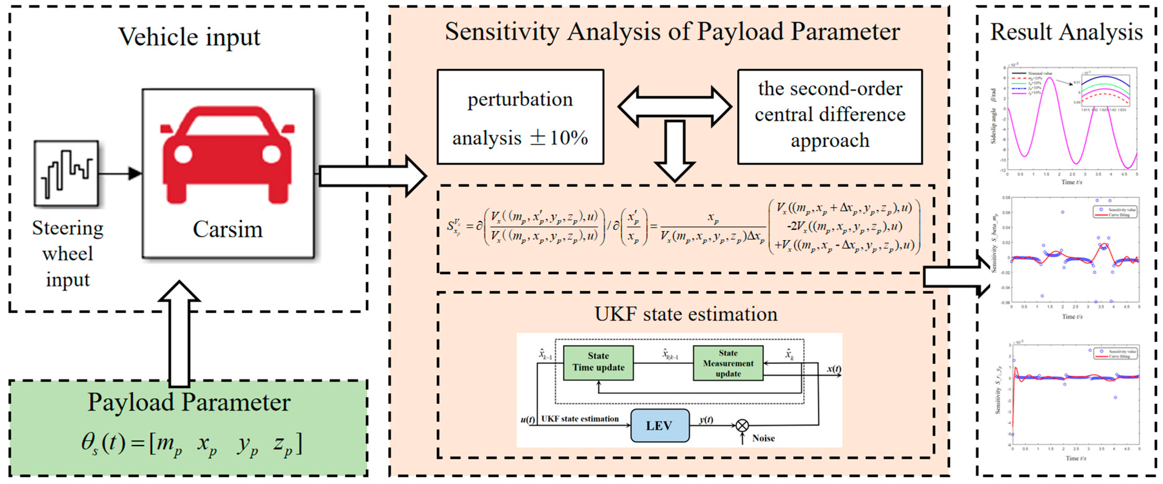
In LEVs, the local sensitivity analysis method, also referred to as the perturbation analysis method [27], entails calculating the model output results following a slight change in the input parameters. The derivative values are then computed to determine the local sensitivity values associated with the input parameters. Due to the difficulty in computing direct differentiation, the finite difference method is used for sensitivity estimates. The fundamental concept of the finite difference technique involves discretizing the solution domain and then approximating the derivative at each discretized point using the difference quotient of the discrete function [28]. This work uses a blend of perturbation analysis and the second-order central difference approach to conduct sensitivity analysis. The subsequent section presents the derivation of the formulas. Figure 3 shows the load parameter sensitivity analysis architecture diagram.
When discussing the vehicle dynamic parameter estimation, the observed outcome may be represented by the variable Y, while the parameters input into the vehicle system can be represented by the vector X. The relationship between the dependent variable Y and the independent variable X may be mathematically stated as:
X = [ x 1 , x 2 , x 3 ,     x n ]
y i = f i ( x ) = f i ( x 1 , x 2 , x 3 ,     x n )
Carry out a Taylor expansion on the aforementioned formula to solve for:
Δ y i = f i ( x 0 + Δ x ) f i ( x 0 ) = d f i ( x 0 ) + 1 2 d 2 f i ( x 0 ) + + 1 n d n f i ( x 0 ) + 1 ( n + 1 ) ! d n + 1 f i ( x 0 + θ Δ x )   i = 1 , 2 , 3     n
The partial derivative at xi reflects its sensitivity as:
S i = y i x i | x = x n   i = 1 , 2 , 3     n
where Si represents the sensitivity with respect to the parameter xi.
In the input vector X, the different units of each parameter xi lead to inconsistent dimensions; therefore, standardization is introduced with dimensionless variables as follows:
S i = y i y i x i x i | x = x n = y i y i δ   i = 1 , 2 , 3     n
where δ represents the perturbation magnitude of the parameter xi.
The specific form of the central difference with a step size of Δx at the points Xi+0.5 and Xi−0.5 is defined as follows:
Δ y i + 0.5 = y i x i y ( X i + 1 ) y ( X i ) Δ x i   , i = 1 , 2 , 3     n
Δ y i 0.5 = y i x i y ( X i ) y ( X i 1 ) Δ x i   , i = 1 , 2 , 3     n
In this context, Xi+1, Xi, and Xi−1 represent the difference terms.
When performing a central difference operation on the two first-order central difference points, the second-order central difference is obtained as follows:
Δ 2 y i = Δ y i + 0.5 Δ y i 0.5 y ( X i + 1 ) y ( X i ) Δ x i y ( X i ) y ( X i 1 ) Δ x i   , i = 1 , 2 , 3     n

3.2. LEV Payload Parameter Sensitivity

The state quantities of the vehicle model are defined as follows:
x s ( t ) = [ V x   β   r z   φ ]
The vehicle load parameters for perturbation analysis are defined as follows:
θ s ( t ) = [ m p   x p   y p   z p ]
Illustrating the derivation process of longitudinal velocity Vx and the sideslip angle β, the model’s trajectory sensitivity is determined by considering the definitions of different payload parameters. Specifically, the trajectory sensitivity of Vx to the payload parameter θs can be expressed as:
S m p V x = V x ( ( m p , x p , y p , z p ) , u ) V x ( ( m p , x p , y p , z p ) , u ) / m p m p = m p V x ( m p , x p , y p , z p ) Δ m p V x ( ( m p + Δ m p , x p , y p , z p ) , u ) - 2 V x ( ( m p , x p , y p , z p ) , u ) + V x ( ( m p - Δ m p , x p , y p , z p ) , u )
S x p V x = V x ( ( m p , x p , y p , z p ) , u ) V x ( ( m p , x p , y p , z p ) , u ) / x p x p = x p V x ( m p , x p , y p , z p ) Δ x p V x ( ( m p , x p + Δ x p , y p , z p ) , u ) - 2 V x ( ( m p , x p , y p , z p ) , u ) + V x ( ( m p , x p - Δ x p , y p , z p ) , u )
S y p V x = V x ( ( m p , x p , y p , z p ) , u ) V x ( ( m p , x p , y p , z p ) , u ) / y p y p = y p V x ( m p , x p , y p , z p ) Δ y p V x ( ( m p , x p , y p + Δ y p , z p ) , u ) - 2 V x ( ( m p , x p , y p , z p ) , u ) + V x ( ( m p , x p , y p - Δ y p , z p ) , u )
S z p V x = V x ( ( m p , x p , y p , z p ) , u ) V x ( ( m p , x p , y p , z p ) , u ) / z p z p = z p V x ( m p , x p , y p , z p ) Δ z p V x ( ( m p , x p , y p , z p + Δ z p ) , u ) - 2 V x ( ( m p , x p , y p , z p ) , u ) + V x ( ( m p , x p , y p , z p - Δ z p ) , u )
Since the solution is obtained after discretization, the local sensitivity values for each step are iteratively accumulated and averaged to further analyze:
S ¯ m p V x = 1 n u = 1 n S m p V x = 1 n u = 1 n V x ( ( m p , x p , y p , z p ) , u ) V x ( ( m p , x p , y p , z p ) , u ) / m p m p
S ¯ x p V x = 1 n u = 1 n S x p V x = 1 n u = 1 n V x ( ( m p , x p , y p , z p ) , u ) V x ( ( m p , x p , y p , z p ) , u ) / x p x p
S ¯ y p V x = 1 n u = 1 n S y p V x = 1 n u = 1 n V x ( ( m p , x p , y p , z p ) , u ) V x ( ( m p , x p , y p , z p ) , u ) / y p y p
S ¯ z p V x = 1 n u = 1 n S z p V x = 1 n u = 1 n V x ( ( m p , x p , y p , z p ) , u ) V x ( ( m p , x p , y p , z p ) , u ) / z p z p
where S m p V x , S x p V x , S y p V x , S z p V x represent the sensitivities of the longitudinal velocity to the payload parameters; S ¯ m p V x , S ¯ x p V x , S ¯ y p V x , S ¯ z p V x represent the average sensitivities of the longitudinal velocity to the payload parameters.
The trajectory sensitivity of β to payload parameter θs is as follows:
S m p β = β ( ( m p , x p , y p , z p ) , u ) β ( ( m p , x p , y p , z p ) , u ) / m p m p = m p β ( m p , x p , y p , z p ) Δ m p β ( ( m p + Δ m p , x p , y p , z p ) , u ) - 2 β ( ( m p , x p , y p , z p ) , u ) + β ( ( m p - Δ m p , x p , y p , z p ) , u )
S x p β = β ( ( m p , x p , y p , z p ) , u ) β ( ( m p , x p , y p , z p ) , u ) / x p x p = x p β ( m p , x p , y p , z p ) Δ x p β ( ( m p , x p + Δ x p , y p , z p ) , u ) - 2 β ( ( m p , x p , y p , z p ) , u ) + β ( ( m p , x p - Δ x p , y p , z p ) , u )
S y p β = β ( ( m p , x p , y p , z p ) , u ) β ( ( m p , x p , y p , z p ) , u ) / y p y p = y p β ( m p , x p , y p , z p ) Δ y p β ( ( m p , x p , y p + Δ y p , z p ) , u ) - 2 β ( ( m p , x p , y p , z p ) , u ) + β ( ( m p , x p , y p - Δ y p , z p ) , u )
S z p β = β ( ( m p , x p , y p , z p ) , u ) β ( ( m p , x p , y p , z p ) , u ) / z p z p = z p β ( m p , x p , y p , z p ) Δ z p β ( ( m p , x p , y p , z p + Δ z p ) , u ) - 2 β ( ( m p , x p , y p , z p ) , u ) + β ( ( m p , x p , y p , z p - Δ z p ) , u )
Since the solution is obtained after discretization, the local sensitivity values for each step are iteratively accumulated and averaged to further analyze:
S ¯ m p β = 1 n u = 1 n S m p β = 1 n u = 1 n β ( ( m p , x p , y p , z p ) , u ) β ( ( m p , x p , y p , z p ) , u ) / m p m p
S ¯ x p β = 1 n u = 1 n S x p β = 1 n u = 1 n β ( ( m p , x p , y p , z p ) , u ) β ( ( m p , x p , y p , z p ) , u ) / x p x p
S ¯ y p β = 1 n u = 1 n S y p β = 1 n u = 1 n β ( ( m p , x p , y p , z p ) , u ) β ( ( m p , x p , y p , z p ) , u ) / y p y p
S ¯ z p β x = 1 n u = 1 n S z p β = 1 n u = 1 n β ( ( m p , x p , y p , z p ) , u ) β ( ( m p , x p , y p , z p ) , u ) / z p z p
where S m p β , S x p β , S y p β , S z p β represent the sensitivities of the longitudinal velocity to the payload parameters; S ¯ m p β , S ¯ x p β , S ¯ y p β , S ¯ z p β x represent the average sensitivities of the longitudinal velocity to the payload parameters.
In summary, the sensitivity calculation process of this paper can be summarized in three steps:
(1).
Based on the definition of partial derivatives, a high-precision numerical differentiator is constructed using the second-order central difference method (Formulas (34)–(38)), and the parameters are dimensionless to ensure comparability.
(2).
For each state variable of interest (such as V x ,   β ) and each load parameter (such as m p ,   x p ), at each simulation time step k, the instantaneous sensitivity trajectory of the time-varying state is calculated by executing the steps described in Formulas (41)–(44) and (49)–(52).
(3).
To further quantify the overall impact of the parameters, the arithmetic mean of the instantaneous sensitivity trajectory is calculated over the entire simulation time domain (Formulas (45)–(48) and (53)–(56)). The obtained results are used for subsequent sensitivity ranking and analysis.
Since the additional trajectory sensitivities S θ s r z , S θ s φ and the average values of trajectory sensitivities S ¯ θ s r z , S ¯ θ s φ can be obtained using the same method, this paper will not provide a detailed explanation of these processes and derivations. By utilizing the definitions and analysis given above, it is possible to ultimately acquire and examine the sensitivity solution for the LEV payload parameters.

4. Design of Vehicle State Observer System

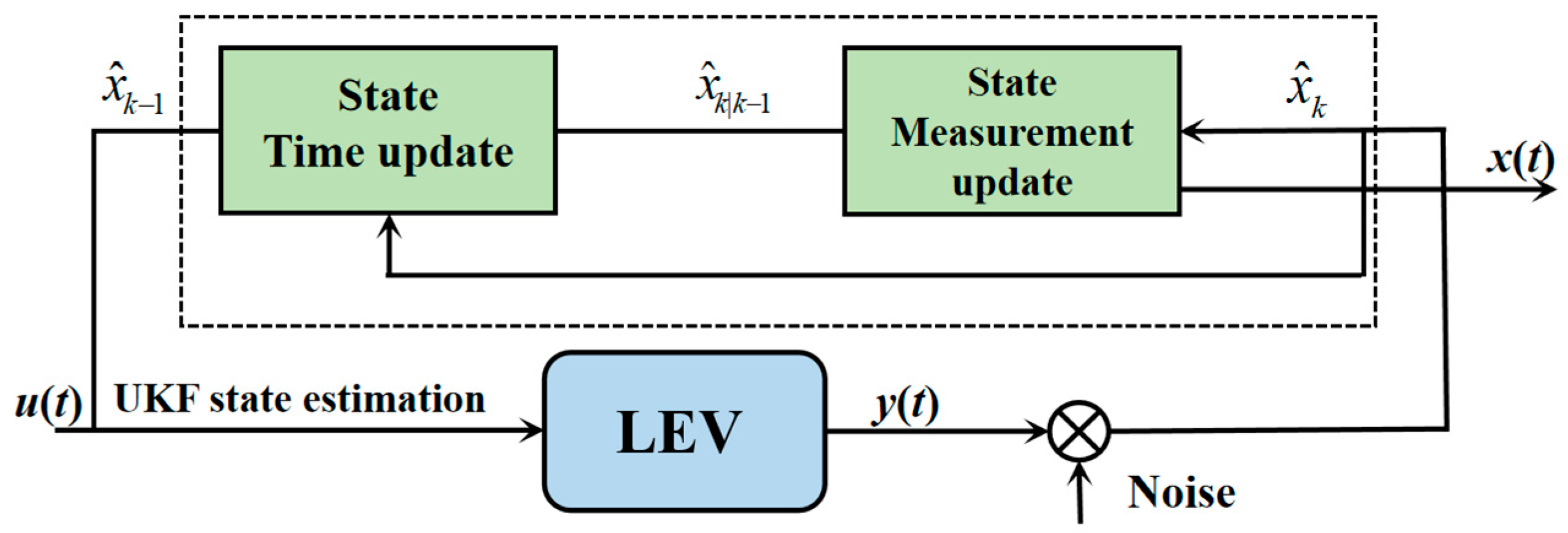
In the meantime, the state estimation system is designed. Figure 4 shows the specific flow chart of the estimation system.
The system for estimating the precise state of vehicle dynamics is outlined as follows:
x ˙ ( t ) = g ( u ( t ) , x ( t ) ) + w ( t ) y ( t ) = f ( x ( t ) ) + v ( t )
where f(·), g(·) are nonlinear functions constructed within the dynamics model of a distributed drive electric vehicle. The input vector is u(t), the state vector is x(t), and v(t) and w(t) are uncorrelated Gaussian white noises with a mean of 0.
Establish the state vector of the Unscented Kalman Filter (UKF) estimation system, which includes the longitudinal velocity, the sideslip angle, the yaw rate, the roll rate, and the roll angle:
x ( t ) = [ V x , β , r z , r x , φ ] T
The input parameters are as follows:
u ( t ) = δ f , ω i j , T d i j T
The measurement vector is chosen based on parameters that are easily measurable or observable by sensors, namely the yaw rate and the roll angle as the measurement vector:
y ( t ) = r z , φ T
Discretize the state vector in the estimation system:
x ( t ) = V x ( t ) β ( t ) r z ( t ) r x ( t ) φ ( t ) = T s ( a x + β ( t 1 ) V x ( t ) r z ( t 1 ) + V x ( t 1 ) a y ( t 1 ) V x ( t 1 ) r z ( t 1 ) β ( t 1 ) a x ( t 1 ) β ( t 1 ) 2 V x ( t 1 ) r z ( t 1 ) / V x ( t 1 ) r z ( t 1 ) + T s [ I x z 0 I z 0 I x 0 I x z 0 2 M x ( t 1 ) + I z 0 I z 0 I x 0 I x z 0 2 M z ( t 1 ) ] r x ( t 1 ) + T s [ I x z 0 I z 0 I x 0 I x z 0 2 M z ( t 1 ) + I z 0 I z 0 I x 0 I x z 0 2 M x ( t 1 ) ] φ ( t 1 ) + r x ( t 1 ) T s
where
M x ( t 1 ) = m s g h r sin φ ( t 1 ) + m s a y ( t 1 ) h r K φ φ ( t 1 ) β φ φ ˙ ( t 1 )
M z ( t 1 ) = l f 0 K α ( α f l ( t 1 ) + α f r ( t 1 ) ) l r 0 K α ( α r l ( t 1 ) + α r r ( t 1 ) )
The UKF estimation system has been set up. The UKF, which eliminates the need to compute complex Jacobian matrices, demonstrates more robust and precise handling of system nonlinearities—including those arising from the Pacejka tire model—compared to the Extended Kalman Filter (EKF). To achieve accurate estimation of key states in light electric vehicles, this study builds upon the strongly nonlinear dynamic model established in Section 2. The state vector is designed to include variables critical for active safety control but difficult to measure directly—such as longitudinal velocity and sideslip angle—while readily measurable quantities like yaw rate and roll angle are treated as observations, thereby it forms an efficient and reliable estimation system. The process noise covariance matrix Q and the measurement noise covariance matrix R were initially set based on prior knowledge of sensor noise characteristics and model uncertainty. Subsequently, Q and R are manually fine-tuned and determined through a series of simulation experiments with the goal of minimizing state estimation error.

5. Simulation Result and Analysis

This part presents a simulation analysis that is carried out to evaluate the effectiveness of the proposed sensitivity solution method. Prior to validation and trajectory sensitivity solving, choose the rated parameters of the payload and apply perturbations of +10% and −10% during the simulation procedure. A perturbation range of ±10% is a common and reasonable range used in engineering sensitivity analysis. It effectively observes the impact of parameter changes while preventing the model from entering a highly nonlinear singular region due to excessive perturbations. The simulation settings are presented in Table 2, which displays the rated parameters of the payload and other selected parameters for the vehicle model in Carsim. Furthermore, because the simulation is performed with a fixed model and inputs, the resulting sensitivity trajectory is deterministic.
This study used Carsim and Matlab/Simulink to establish a joint simulation platform based on three main considerations: Utilizing Carsim, an industry-recognized high-fidelity dynamics simulation software, provided a reliable “virtual testing ground” for verifying the effectiveness of the proposed method, significantly enhancing the credibility of the results; the platform enabled us to focus on developing novel sensitivity analysis algorithms in Matlab/Simulink without having to build complex vehicle models from scratch, thereby improving research efficiency; and verification in this highly realistic environment strongly demonstrated the practical value and potential applicability of this research to actual light electric vehicle controller design.
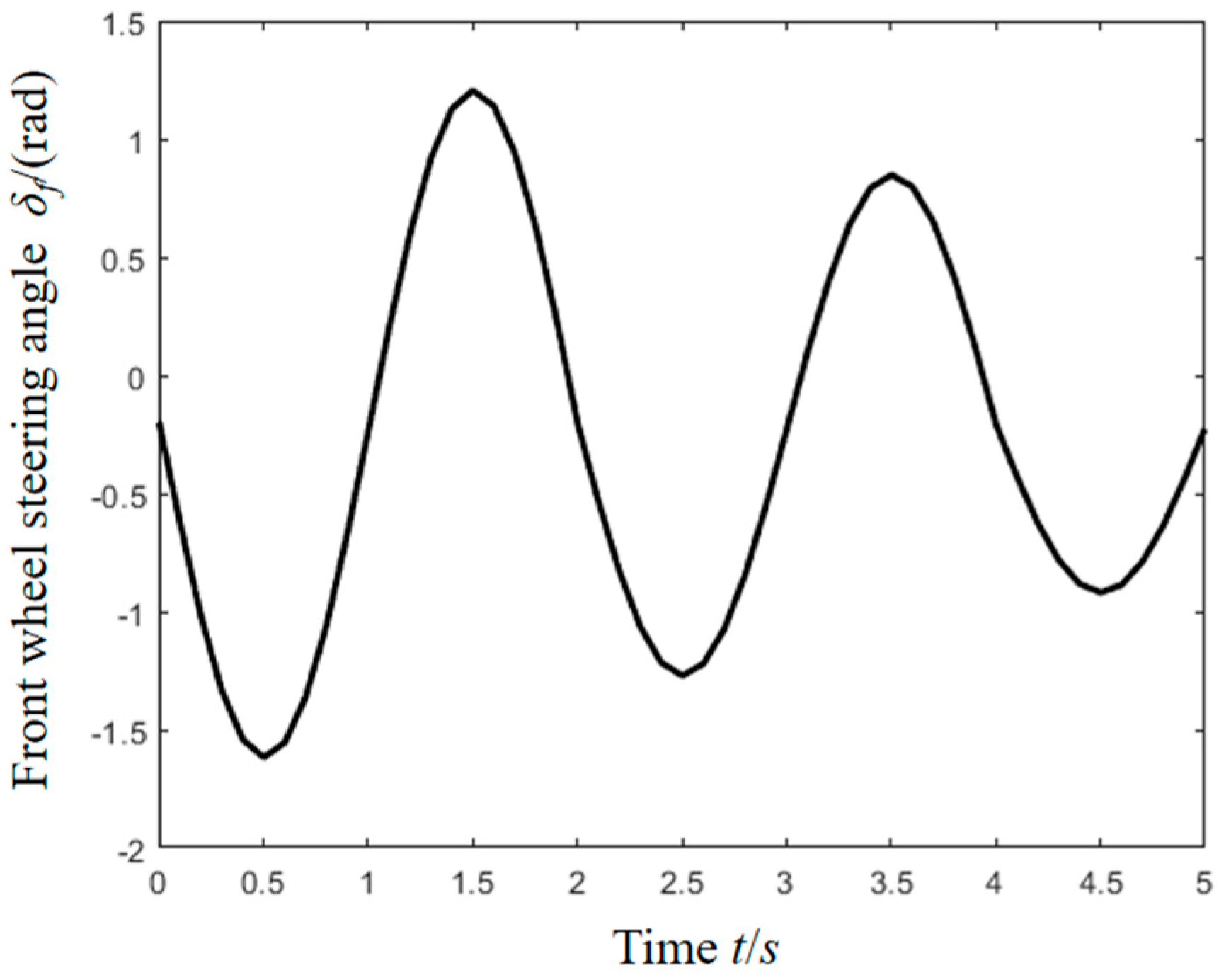
The integrated simulation platform environment consists of Carsim 2019.1 and Matlab R2018a. The simulation scenario employs a sine wave condition with varying amplitude. The steering angle exhibits a sinusoidal waveform with fluctuating amplitude, while the vehicle’s beginning velocity is 30 km/h and experiences a specific deceleration while braking. The overall duration of the simulation is 5 s. Figure 5 displays the input signal for the front wheel steering angle, which is utilized in the UKF estimate system to determine the vehicle condition.
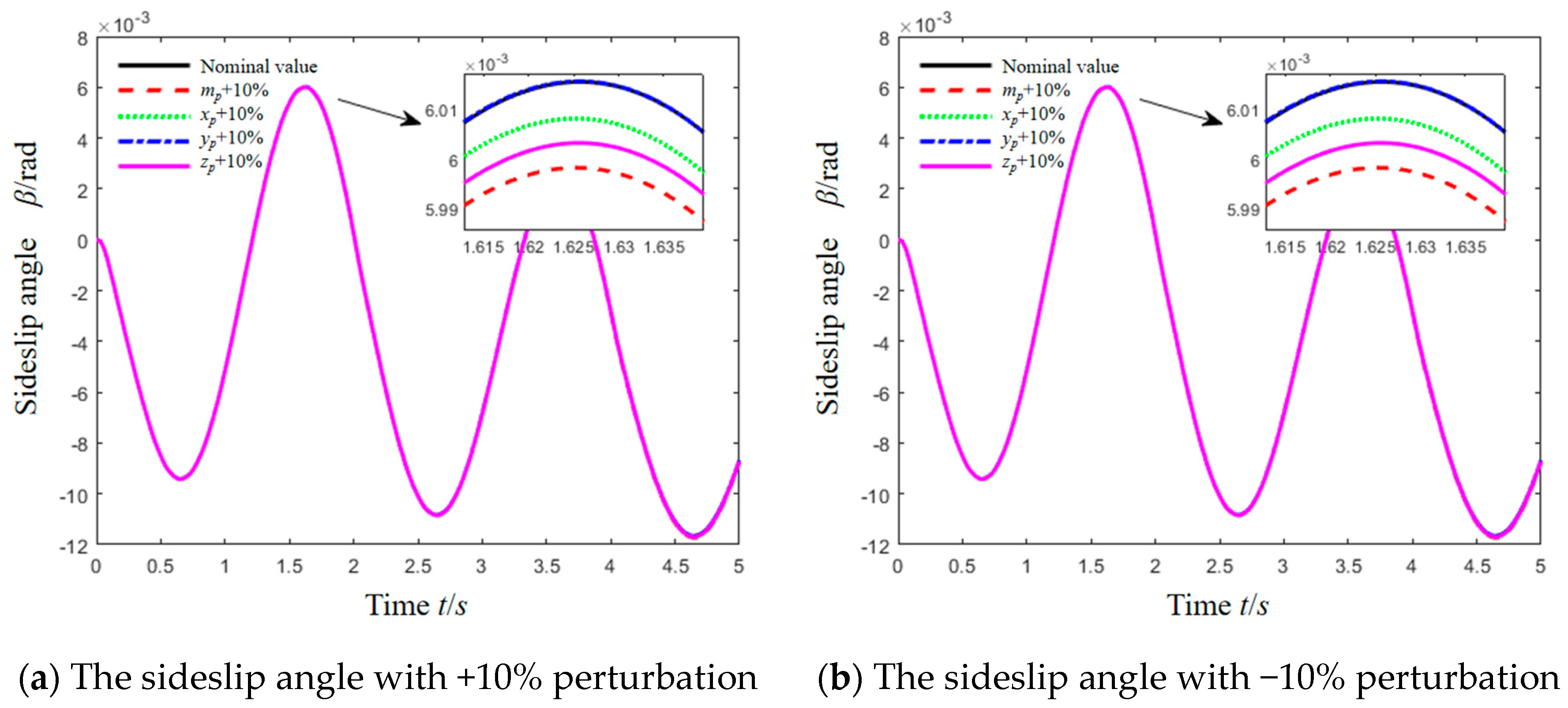
The simulation results for the sideslip angle under the amplitude sine condition are displayed in Figure 6. The perturbation of the four payload parameters allows for accurate estimation of the sideslip angle. It is evident that the UKF estimation results still exhibit a slight variation from the rated values in the presence of parameter perturbation.
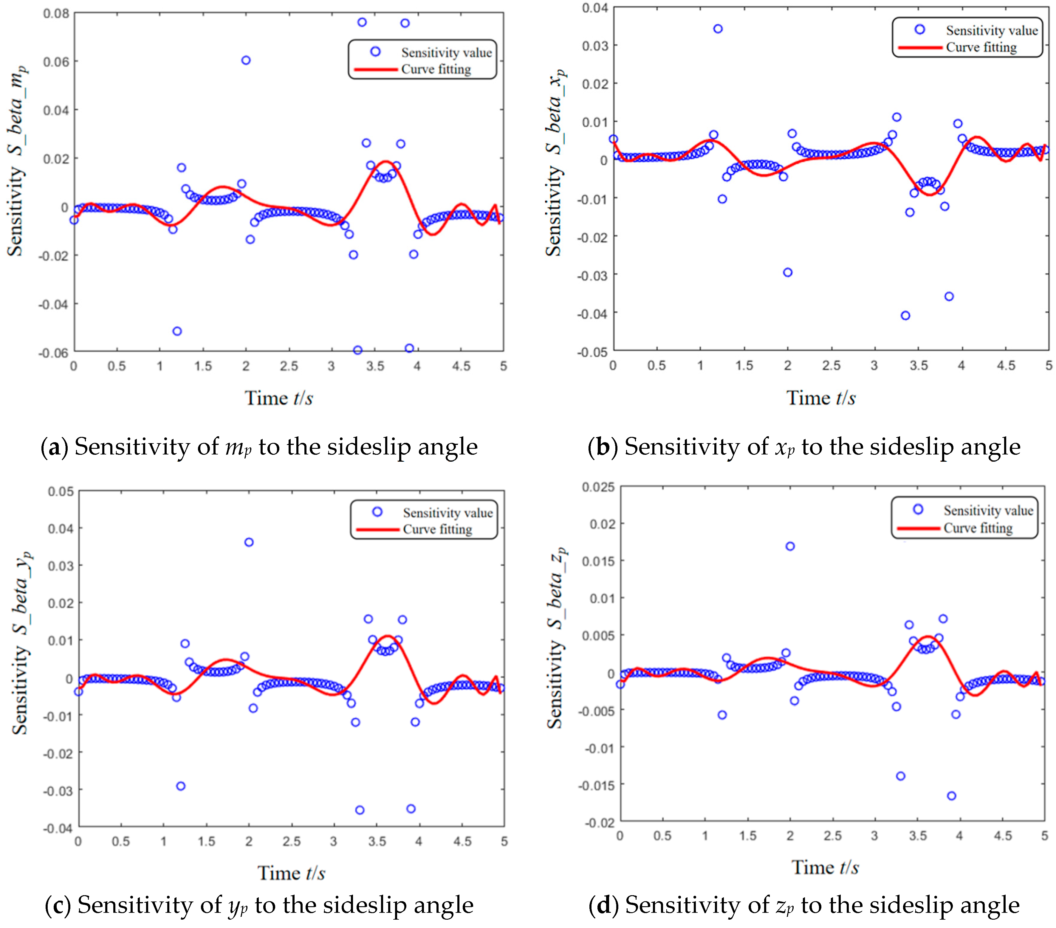
Figure 7 displays the study and calculation findings of the vehicle’s sensitivity to the four payload parameters in terms of the sideslip angle. The sensitivity values are depicted as circle dots. In order to more effectively examine the changes in sensitivity over time in the simulation, a polynomial fitting curve is employed to accurately depict the fitting results of the sensitivity values. It is evident that the sensitivity values will vary when the direction of the steering excitation varies. While the simulation process may experience oscillations, the sensitivity levels remain pretty steady overall.
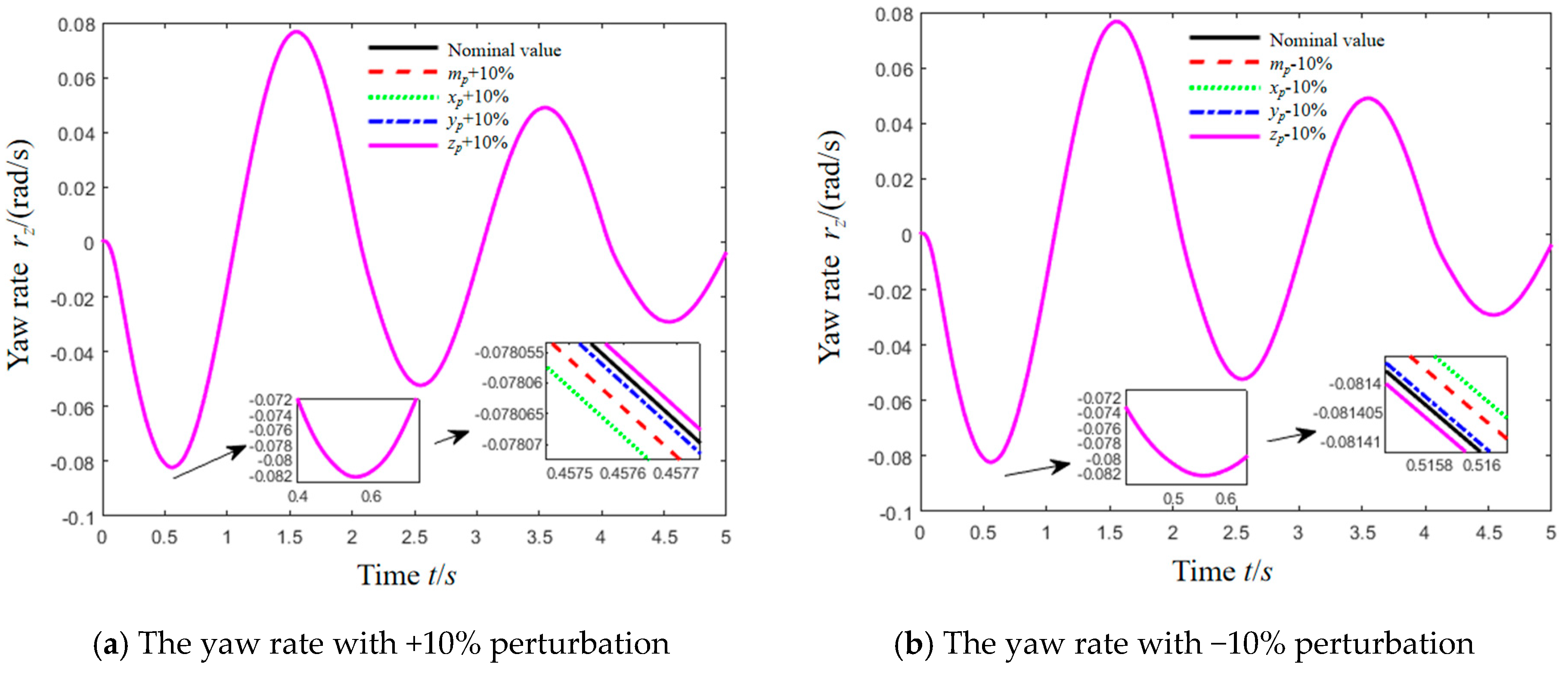
The estimation results of the yaw rate, which is a state quantity that can be plainly observed, are demonstrated in Figure 8 and indicate good performance of the Unscented Kalman Filter (UKF). Nevertheless, when subjected to various perturbations in the payload parameter, the UKF estimation results still exhibit some degree of error. Upon closer examination, it is observed that the yaw rate is very responsive to small variations in the longitudinal position of the payload xp. It is then influenced by the payload mass mp, but to a lesser extent. The perturbations in the other two payload variables have a minimal impact on the yaw rate.
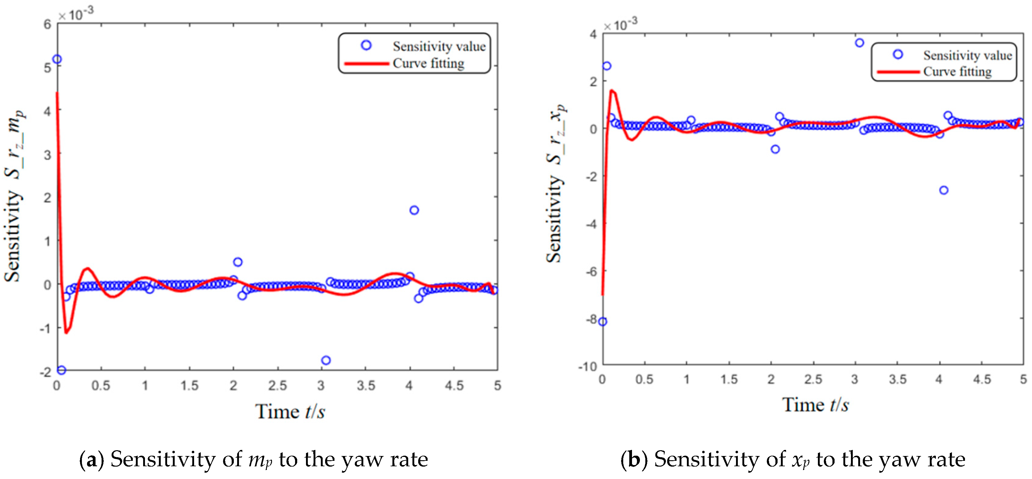
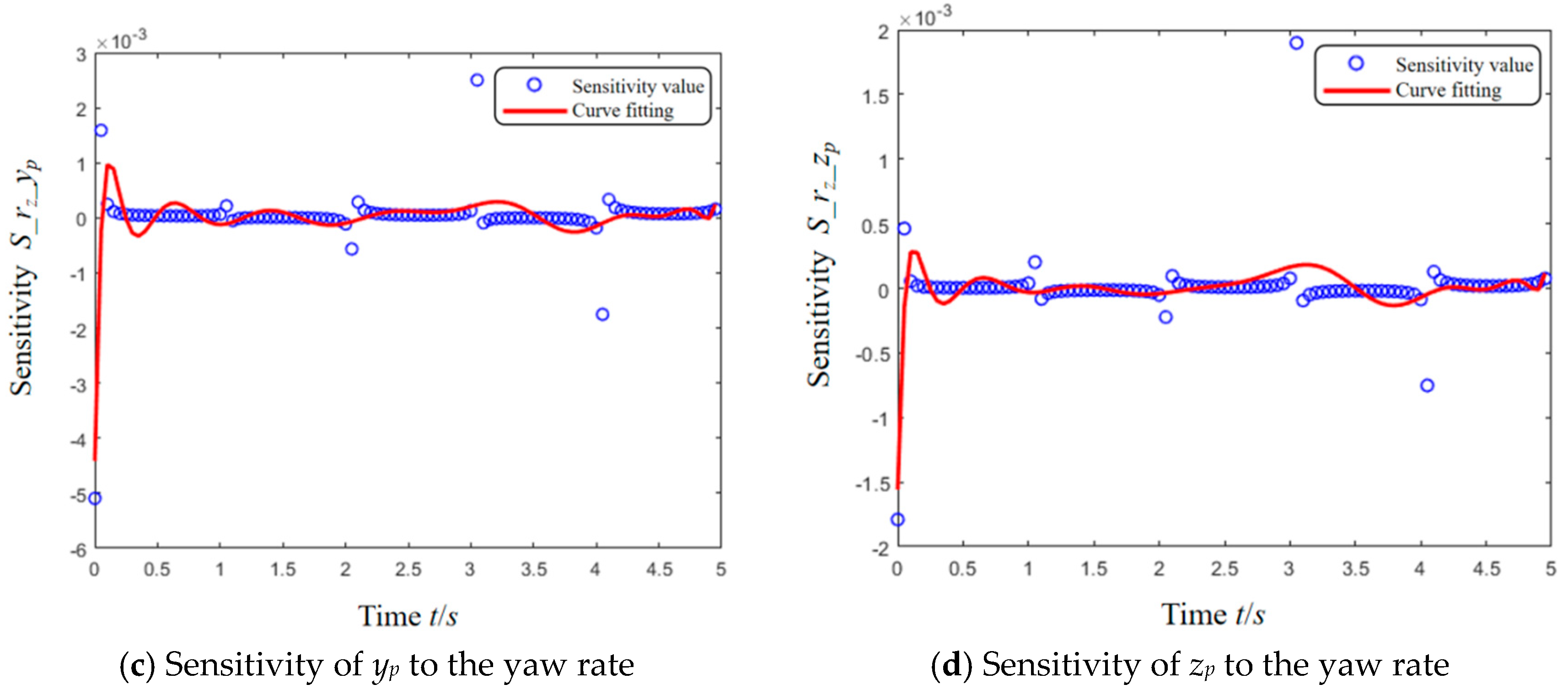
Figure 9 displays the study and calculation outcomes of the vehicle’s sensitivity to yaw rate in relation to the four payload parameters. Initially, the sensitivity values to the four payload parameters are all relatively high. However, as the simulation progresses, these sensitivity values progressively reach a stable state.
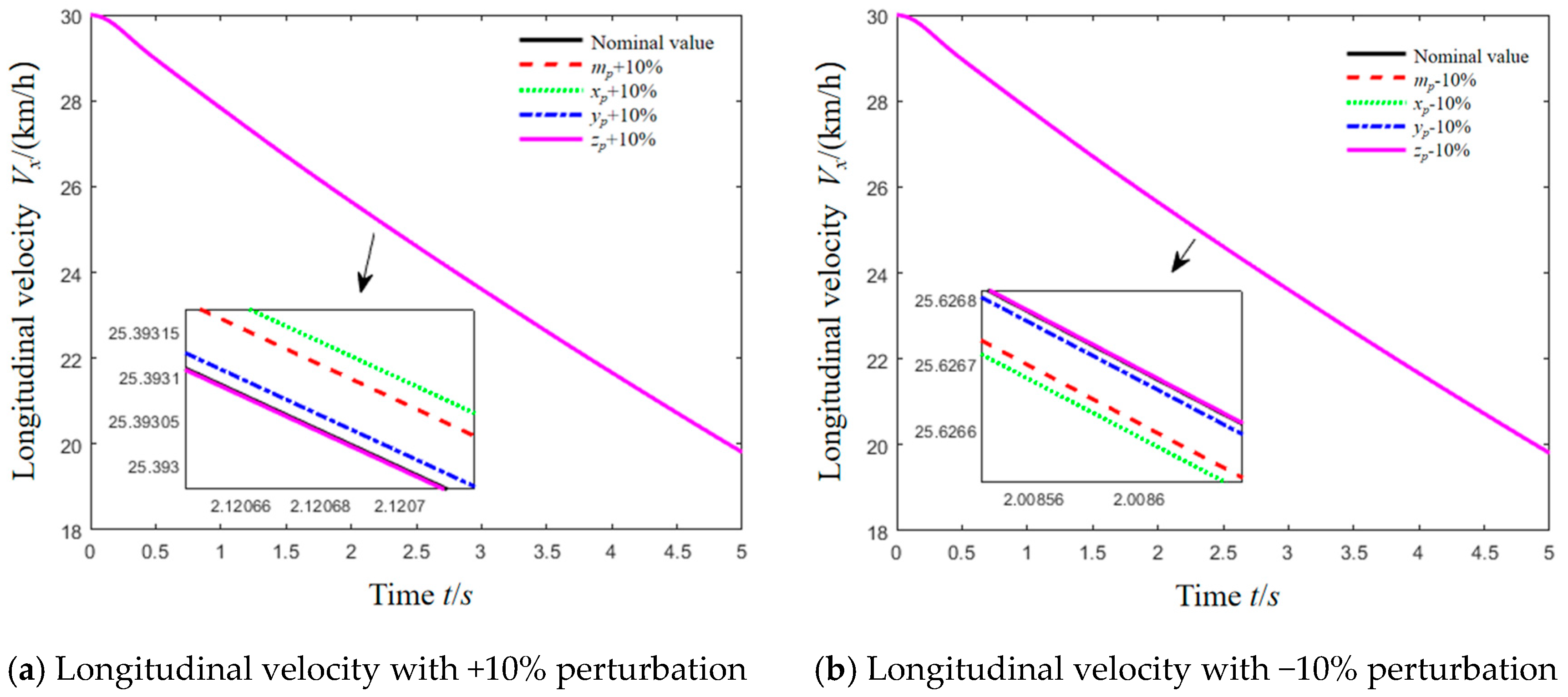
The UKF approach offers a reliable estimate of the longitudinal velocity, as seen by the simulation results illustrated in Figure 10. Upon close examination of the magnified local view, it is evident that the longitudinal velocity is very responsive to even minor alterations in the longitudinal location of the payload xp, and is also significantly influenced by the mass of the payload mp. The impact of the other two payload variables, particularly the vertical position of the payload zp, is rather little. In the magnified image, the vertical position remains extremely close to the rated value, suggesting that its influence on the estimation findings of longitudinal velocity is modest.
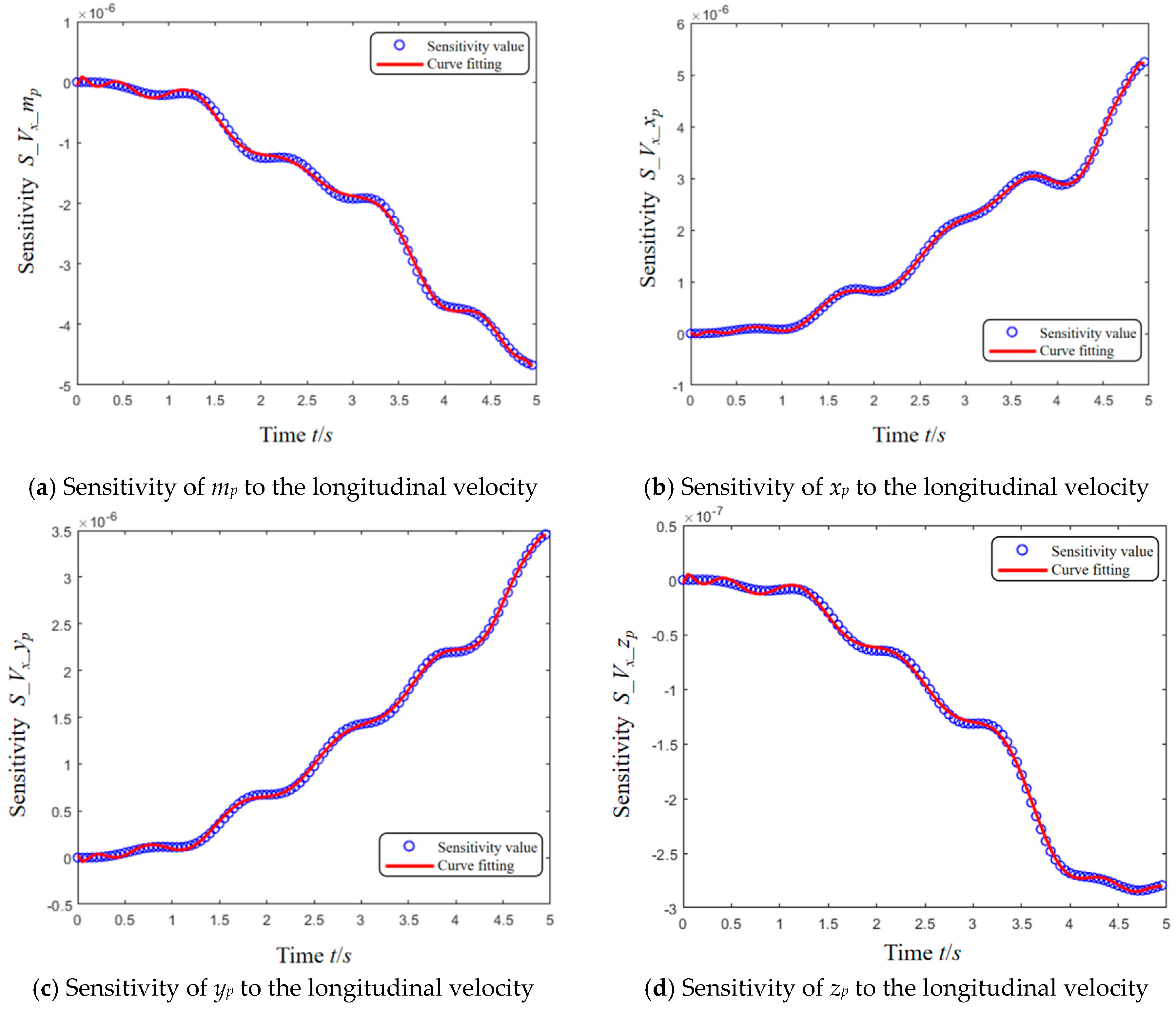
Figure 11 displays the analysis and calculation outcomes of the vehicle’s sensitivity to longitudinal velocity in relation to the four payload characteristics. The sensitivity values have been fitted with a continuous curve, exhibiting a progressive increase as the simulation period progresses. However, when compared to the sensitivity values of other state quantities, the sensitivity values of longitudinal velocity are relatively smaller. This suggests that the UKF technique has a more accurate estimation effect on longitudinal velocity.
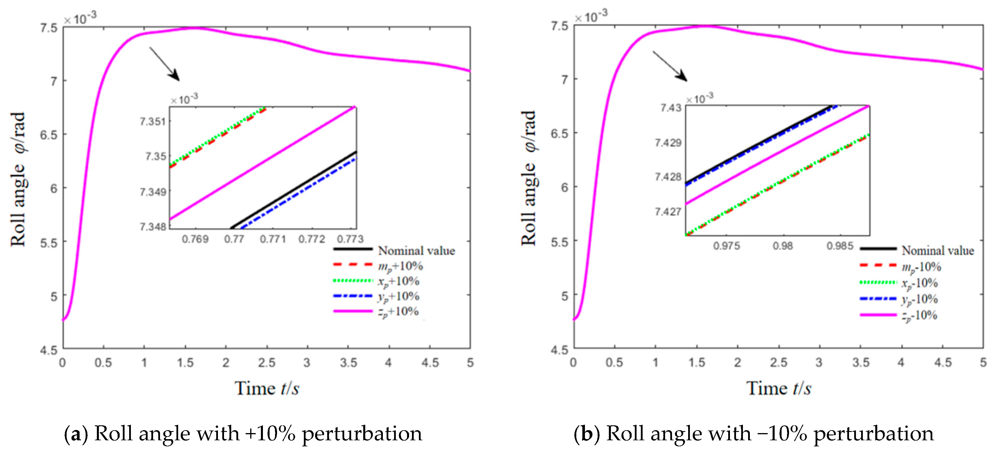
Figure 12 displays the simulation outcomes of the UKF for the roll angle of the vehicle. Regardless of disturbances in various payload characteristics, the vehicle’s roll angle can still be accurately anticipated.
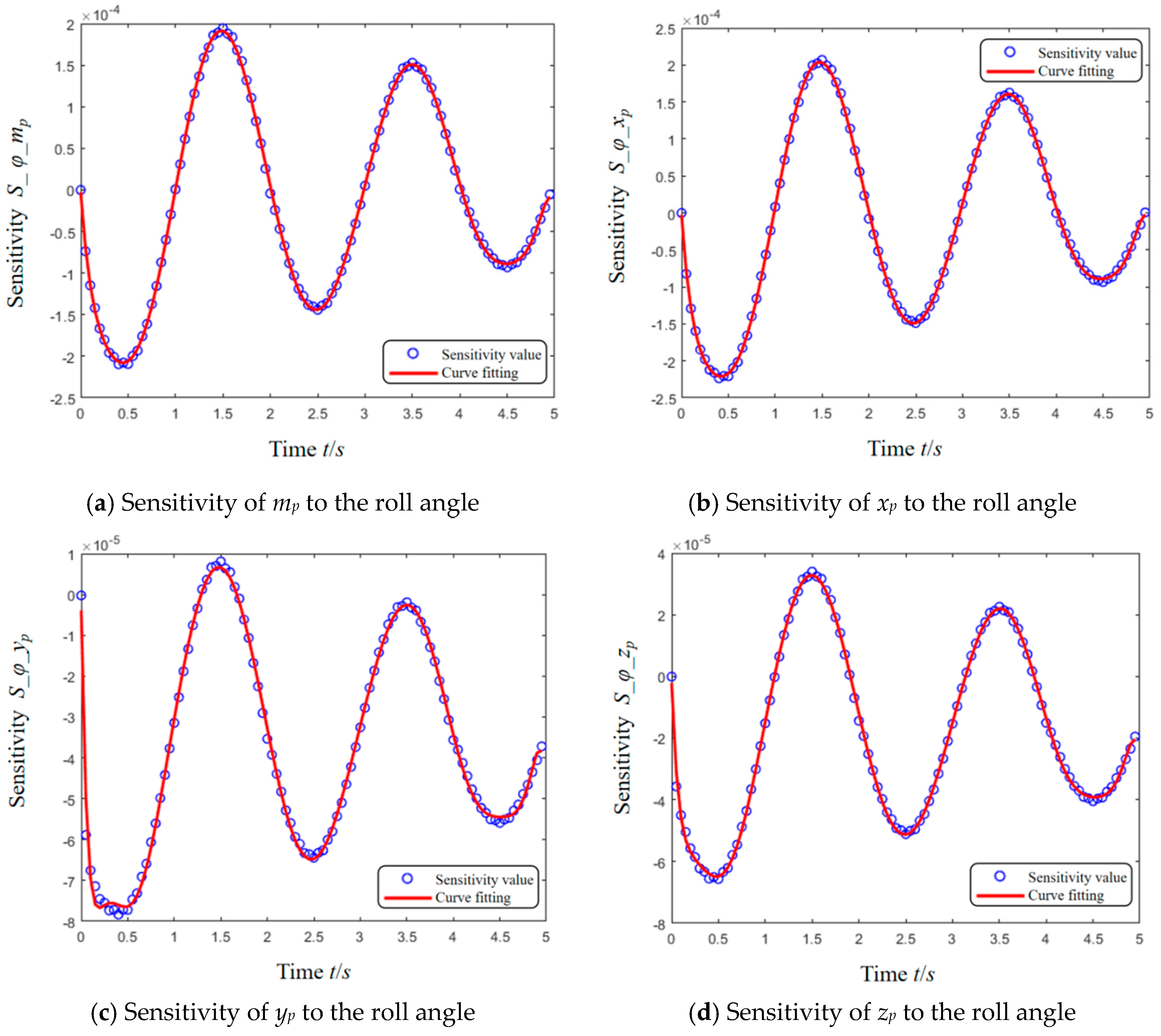
Figure 13 displays the study and calculation outcomes of the vehicle’s sensitivity to the four payload factors in terms of roll angle. Upon observing the fitting curves, it becomes evident that the sensitivity values for the payload mass mp and longitudinal position xp exhibit strong fitting effects. The sensitivity values for the lateral position yp and vertical position zp of the payload exhibit inadequate fitting at the start of the simulation. However, as the simulation advances, the fitting of the sensitivity values for the state estimation procedure steadily improves.
Table 3 presents the average outcomes of the sensitivity study of vehicle states to payload characteristics. This analysis is conducted to assess the extent to which state quantities are influenced by various payload factors. When estimating the sideslip angle of the center of gravity, the most sensitive factor is the mass of the payload mp. The longitudinal position xp and lateral position yp of the payload also have some impact, while the vertical position zp of the payload has the least influence. When estimating the yaw rate, the payload’s longitudinal position xp has the greatest impact on the estimation. The payload’s mass mp and lateral position yp also have some influence, while the payload’s vertical position zp has the least impact. Based on the sensitivity analysis of the longitudinal velocity, it is evident that the payload mass mp is the most sensitive to the estimation effect of the longitudinal velocity. The payload longitudinal position xp is the next most sensitive, while the payload lateral position yp also has a noticeable impact. On the other hand, the influence of the payload vertical position zp is the least significant. When predicting the roll angle, the sensitivity mean values for the longitudinal position of the payload xp and the mass of the payload mp show no significant difference. However, the roll angle is highly sensitive to both of these factors. The impact of the payload’s lateral position yp and vertical position zp is rather minor and significantly less than the previous two factors.
Sensitivity analysis of the four UKF-estimated observations reveals that for the slip angle, the load parameter sensitivity follows the order mp > xpyp >> zp; for the yaw rate, the load parameter sensitivity follows the order xp > mp > yp > zp; for the longitudinal velocity, the load parameter sensitivity follows the order mpxp > yp>>zp; and for the roll angle, the load parameter sensitivity follows the order mpxp >> yp > zp. For a vehicle dynamics model with varying load mass, even small perturbations can affect the estimation, while the longitudinal and lateral positions of the applied load also have an impact. The established vehicle model is insensitive to vertical loads.
The sensitivity analysis results of the UKF estimated observation quantities mentioned above reveal the sensitivity levels of payload parameters for different vehicle states. This analysis is crucial for understanding the impact of changes in load parameters on vehicle dynamics. When developing adaptive state observers or controllers, online identification of these key parameters or designing robust control laws should be prioritized. This is crucial for improving the accuracy of state estimation algorithms like the UKF. Furthermore, the proposed sensitivity analysis method is based on forward simulation, which is much faster than real-time simulation. While implementing the entire analysis process in a real-time vehicle control system is currently challenging, the offline analysis results can be directly used to simplify control-oriented models or provide priority guidance for adaptive parameter estimation modules, which has important practical value for resource-limited vehicle control units.

6. Conclusions

This paper introduces a new way for analyzing the sensitivity of payload parameters to the reaction of the LEV system. The method allows for a quantitative observation of this sensitivity. A dynamic model of LEV system is developed, which focuses on analyzing variations in payload parameters. The UKF approach is employed to estimate the state of the vehicle model, while sensitivity analysis is performed by integrating perturbation analysis with the second-order central difference method. The simulation results demonstrate that the suggested method can precisely depict the correlation between LEV payload parameters and system state estimation. In the future, additional research will be conducted to compare the effects of various sensitivity analysis techniques on the estimator of the LEV system. This study has several limitations. First, it lacks real-world experimental validation, and future work requires testing on a real vehicle. Second, the model makes some simplifying assumptions, and a more complex model will be developed in the future to cover a wider range of operating conditions. Regarding practicality, the results of this study can directly empower on-board LEV control units. By integrating low-cost sensors (such as IMUs, wheel speed sensors, and motor torque/speed sensors) and combining them with efficient parameter identification algorithms (such as RLS), the control unit can estimate or adapt key payload parameters online.

Author Contributions

Conceptualization, X.J., Z.W., Y.T., J.L. (Jianbo Lv), J.L. (Jianning Lu) and N.V.O.I.; supervision, X.J.; conception and design, X.J. and Z.W.; collection and assembly of data, X.J., Z.W.; manuscript writing, X.J., Z.W., Y.T., J.L. (Jianbo Lv), J.L. (Jianning Lu) and N.V.O.I.; funding, X.J. All authors have read and agreed to the published version of the manuscript.

Funding

This work was supported by Natural Science Foundation of Shanghai (Grant No. 25ZR1401118), and the Key Research and Development Program of China Yangtze River Delta (Grant No. 2023CSJGG0900).

Data Availability Statement

Data are contained within the article.

Conflicts of Interest

Zhaoran Wang was employed by the Shanghai Civil Aviation Electromechanical Systems Co., Ltd. The remaining authors declare that the research was conducted in the absence of any commercial or financial relationships that could be construed as a potential conflict of interest.

References

  1. Zhang, H.; Zhang, X.; Wang, J. energy-to-peak control of vehicle lateral dynamics stabilisation. Veh. Syst. Dyn. 2014, 52, 309–340. [Google Scholar] [CrossRef]
  2. Deng, H.; Zhao, Y.; Nguyen, A.T.; Huang, C. Fault tolerant predictive control with deep-reinforcement-learning-based torque distribution for four in-wheel motor drive. IEEE/ASME Trans. Mechatron. 2023, 28, 668–680. [Google Scholar] [CrossRef]
  3. Farazandeh, A.; Ahmed, A.K.W.; Rakheja, S. An independently controllable active steering system for maximizing the handling performance limits of road vehicles. Proc. Inst. Mech. Eng. Part D J. Automob. Eng. 2015, 229, 1291–1309. [Google Scholar] [CrossRef]
  4. Jin, X.; Wang, Q.; Yan, Z.; Yang, H.; Yin, G. Integrated robust control of path following and lateral stability for autonomous in-wheel-motor-driven electric vehicles. Proc. Inst. Mech. Eng. Part D J. Automob. Eng. 2025, 239, 12696–12706. [Google Scholar] [CrossRef]
  5. Perić, S.L.; Antić, D.S.; Milovanović, M.B.; Mitić, D.B.; Milojković, M.T.; Nikolić, S.S. Quasi-sliding mode control with orthogonal endocrine neural network-based estimator applied in anti-lock braking system. IEEE/ASME Trans. Mechatron. 2015, 21, 754–764. [Google Scholar] [CrossRef]
  6. Wei, Z.; Guo, X. An ABS control strategy for commercial vehicle. IEEE/ASME Trans. Mechatron. 2015, 20, 384–392. [Google Scholar] [CrossRef]
  7. Li, H.; Liu, H.; Gao, H.; Shi, P. Reliable fuzzy control for active suspension systems with actuator delay and fault. IEEE Trans. Fuzzy Syst. 2011, 20, 342–357. [Google Scholar] [CrossRef]
  8. Saifia, D.; Chadli, M.; Karimi, H.R.; Labiod, S. Fuzzy control for electric power steering system with assist motor current input constraints. J. Frankl. Inst. 2015, 352, 562–576. [Google Scholar] [CrossRef]
  9. Niu, S.; Yu, H.; Niu, S.; Jian, L. Power Loss Analysis and Thermal Assessment on Wireless Electric Vehicle Charging Technology: The Over-Temperature Risk of Ground Assembly Needs Attention. Appl. Energ. 2020, 275, 115344. [Google Scholar] [CrossRef]
  10. Jia, C.; Liu, W.; He, H.; Chau, K.T. Deep reinforcement learning-based energy management strategy for fuel cell buses integrating future road information and cabin comfort control. Energ. Convers. Manag. 2024, 321, 119032. [Google Scholar] [CrossRef]
  11. Lu, D.; Yi, F.; Hu, D.; Li, J.; Yang, Q.; Wang, J. Online optimization of energy management strategy for FCV control parameters considering dual power source lifespan decay synergy. Appl. Energ. 2023, 348, 121516. [Google Scholar] [CrossRef]
  12. Krishna, T.; Krishna, K.R. Sensitivity analysis of tyre characteristic parameters on ABS performance. Vehicle Syst. Dyn. 2020, 60, 47–72. [Google Scholar] [CrossRef]
  13. Huang, X.; Wang, J. Longitudinal motion based lightweight vehicle payload parameter real-time estimations. J. Dyn. Syst. Meas. Control. 2013, 135, 011–013. [Google Scholar] [CrossRef]
  14. Todeschini, F.; Corno, M.; Panzani, G.; Fiorenti, S.; Savaresi, S.M. Adaptive cascade control of a brake-by-wire actuator for sport motorcycles. IEEE/ASME Trans. Mechatron. 2014, 20, 1310–1319. [Google Scholar] [CrossRef]
  15. Sun, Y.; Li, L.; Yan, B.; Yang, C.; Tang, G. A hybrid algorithm combining EKF and RLS in synchronous estimation of road grade and vehicle׳ mass for a hybrid electric bus. Mech. Syst. Signal Process. 2016, 68, 416–430. [Google Scholar] [CrossRef]
  16. Hong, S.; Lee, C.; Borrelli, F.; Hedrick, J.K. A Novel Approach for Vehicle Inertial Parameter Identification Using a Dual Kalman Filter. IEEE Trans. Intell. Transp. Syst. 2015, 16, 151–161. [Google Scholar] [CrossRef]
  17. Boada, B.L.; Garcia-Pozuelo, D.; Boada, M.J.L.; Diaz, V. A constrained dual Kalman filter based on pdf truncation for estimation of vehicle parameters and road bank angle: Analysis and experimental validation. IEEE Trans. Intell. Transp. Syst. 2016, 18, 1006–1016. [Google Scholar] [CrossRef]
  18. Wan, W.; Feng, J.; Song, B.; Li, X. Huber-Based Robust Unscented Kalman Filter Distributed Drive Electric Vehicle State Observation. Energies 2021, 14, 750. [Google Scholar] [CrossRef]
  19. Lampe, N.; Ziaukas, Z.; Westerkamp, C.; Jacob, H.-G. Analysis of the Potential of Onboard Vehicle Sensors for Model-based Maximum Friction Coefficient Estimation. In Proceedings of the American Control Conference (ACC), San Diego, CA, USA, 31 May–2 June 2023; pp. 1622–1628. [Google Scholar]
  20. Ribeiro, A.M.; Moutinho, A.; Fioravanti, A.R.; de Paiva, E.C. Estimation of Tire-Road Friction for Road Vehicles: A Time Delay Neural Network Approach. J. Braz. Soc. Mech. Sci. Eng. 2019, 42, 4. [Google Scholar] [CrossRef]
  21. Kim, D.J.; Kim, J.S.; Lee, S.H.; Chung, C.C. A Comparative Study of Estimating Road Surface Condition Using Support Vector Machine and Deep Neural Networ. In Proceedings of the IEEE Intelligent Transportation Systems Conference (ITSC), Auckland, New Zealand, 27–30 October 2019; pp. 1066–1071. [Google Scholar]
  22. Grigorescu, S.; Trasnea, B.; Cocias, T.; Macesanu, G. A survey of deep learning techniques for autonomous driving. J. Field Robot. 2020, 37, 362–386. [Google Scholar] [CrossRef]
  23. Baffet, G.; Charara, A.; Lechner, D. Experimental evaluation of a sliding mode observer for tire-road forces and an extended Kalman filter for vehicle sideslip angle. In Proceedings of the 46th IEEE Conference on Decision and Control, New Orleans, LA, USA, 12–14 December 2007; pp. 3877–3882. [Google Scholar]
  24. Yang, X.; Wang, Z.; Peng, W. Coordinated control of AFS and DYC for vehicle handling and stability based on optimal guaranteed cost theory. Vehicle Syst. Dyn. 2009, 47, 57–79. [Google Scholar] [CrossRef]
  25. Poussot-Vassal, C.; Sename, O.; Dugard, L.; Savaresi, S.M. Vehicle dynamic stability improvements through gain-scheduled steering and braking control. Vehicle Syst. Dyn. 2011, 49, 1597–1621. [Google Scholar] [CrossRef]
  26. Jin, X.; Yin, G.; Chen, N. Advanced estimation techniques for vehicle system dynamic state: A survey. Sensors 2019, 19, 4289. [Google Scholar] [CrossRef]
  27. Callejo, A.; de Jalón, J.G. Vehicle Suspension Identification Via Algorithmic Computation of State and Design Sensitivities. J. Mech. Design 2014, 137, 021403. [Google Scholar] [CrossRef]
  28. Shi, C.; Zhao, C.; Xin, L.; Wang, J. Dynamic impact of unsupported sleepers on railway infrastructure with a coupled MBD-DEM-FDM model. Trans. Geotech. 2024, 45, 101221. [Google Scholar] [CrossRef]
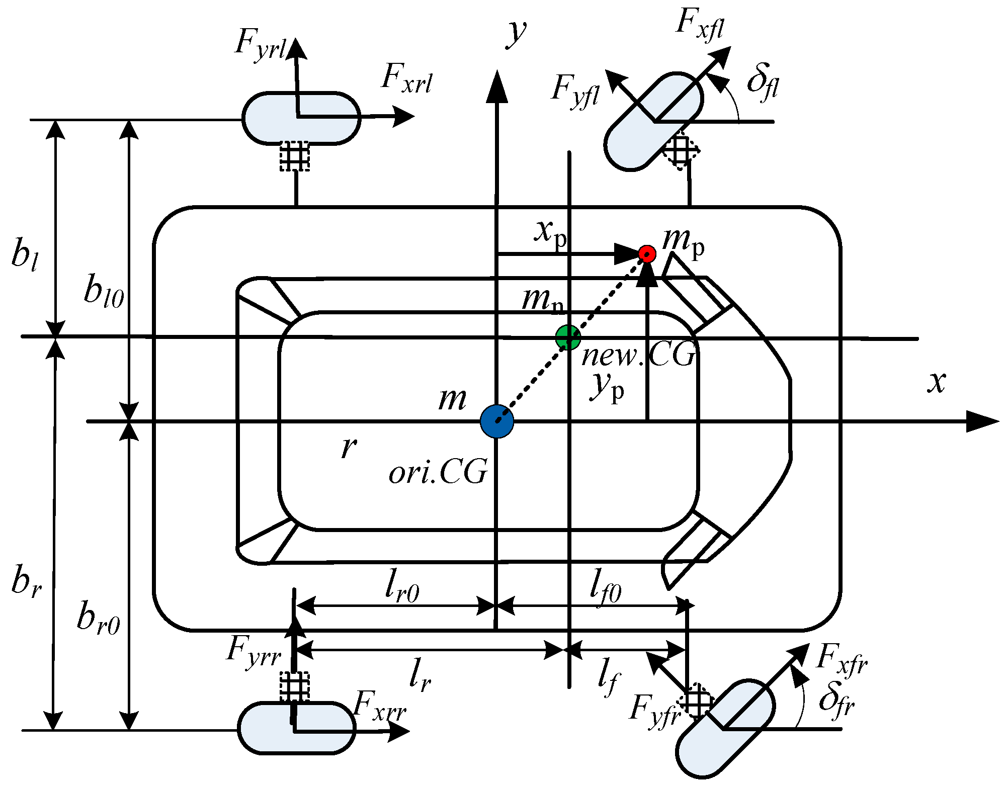
Figure 1. Dynamic model of lightweight electric vehicle.
Electronics 14 04372 g001
Figure 2. Motor and wheel dynamics model.
Electronics 14 04372 g002
Figure 3. Payload parameter sensitivity analysis architecture.
Electronics 14 04372 g003
Figure 4. The estimation system flow chart.
Electronics 14 04372 g004
Figure 5. Vehicle front wheel angle input in amplitude sine condition.
Electronics 14 04372 g005
Figure 6. Estimated results of vehicle sideslip angle.
Electronics 14 04372 g006
Figure 7. Sensitivity analysis of vehicle sideslip angle.
Electronics 14 04372 g007
Figure 8. Estimated results of vehicle yaw rate.
Electronics 14 04372 g008
Figure 9. Sensitivity analysis of vehicle yaw rate.
Electronics 14 04372 g009aElectronics 14 04372 g009b
Figure 10. Estimated results of vehicle longitudinal velocity.
Electronics 14 04372 g010
Figure 11. Sensitivity analysis of vehicle yaw rate.
Electronics 14 04372 g011
Figure 12. Estimated results of vehicle roll angle.
Electronics 14 04372 g012
Figure 13. Sensitivity analysis of vehicle roll angle.
Electronics 14 04372 g013
Table 1. Parameter information in the Pacejka model.
Tire ParametersLongitudinal Tire ForceLateral Tire Force
xsα
C1.651.3
D a 1 F z 2 + a 2 F z b 1 F z 2 + b 2 F z
BCD a 3 F z 2 + a 4 F z e a 5 F z b 3 sin b 4 tan 1 b 5 F z
E a 6 F z 2 + a 7 F z + a 8 b 6 F z 2 + b 7 F z + b 8
Sh a 9 F z + a 10 Y b 9 F z + b 10 Y
Sv a 11 F z γ + a 12 F z + a 13 b 11 F z γ + b 12 F z + b 13
Table 2. Vehicle load and vehicle model parameters.
ParameterValueParameterValue
mn833 kgIz1017 kg·m2
Ix270 kg·m2Iy750 kg·m2
lf1.103 mbl0.7695 m
lr1.250 mbr0.7695 m
mp80 kgyp0.38 m
xp0.62 mzp0.29 m
Vx030 km/hTs0.001 s
Table 3. Average value of sensitivity analysis.
Payload Parameter Changempxpypzp
Sideslip angle ±10%2.1516 × 10−21.1381 × 10−21.1281 × 10−25.2239 × 10−3
Yaw rate ±10%2.9808 × 10−44.2395 × 10−42.6708 × 10−41.0961 × 10−4
Longitudinal velocity ±10%1.7861 × 10−61.7510 × 10−61.2070 × 10−61.1990 × 10−7
Roll angle ±10%1.0177 × 10−41.0708 × 10−43.8248 × 10−53.0009 × 10−5
Disclaimer/Publisher’s Note: The statements, opinions and data contained in all publications are solely those of the individual author(s) and contributor(s) and not of MDPI and/or the editor(s). MDPI and/or the editor(s) disclaim responsibility for any injury to people or property resulting from any ideas, methods, instructions or products referred to in the content.