A Study on Exploiting Temporal Patterns in Semester Records for Efficient Student Dropout Prediction

Abstract

Academic achievement data are essential in building a model to predict student dropout. When an attribute of the data has multiple values, each representing a student’s achievement earned over a semester, existing methods typically calculate a mean from those values and use it to build learning data. Such a summary-based approach has been widely used because it can simplify learning processes, including feature extraction. However, model performance can be further improved if patterns in multiple semester values can be properly extracted and used for learning, instead of using summaries. Despite its potential, this problem has not been investigated in previous studies. In this paper, we demonstrate that recurrent neural networks (RNNs) can effectively be used to exploit the patterns in students’ academic records stored by semester. To identify patterns in the data and find solutions suitable for it, various neural network algorithms were compared. Attention was also adopted to improve model performance. Experiments conducted on real student records showed that the gate recurrent unit (GRU) model with multi-head attention achieved an F1 score of 0.9416, which was approximately 5% higher than the existing summary-based approaches. This demonstrates that the semester records exhibit temporal patterns and RNNs can effectively be used to exploit these patterns.

1. Introduction

Student dropout has been widely recognized as one of the most multifaceted and pressing challenges facing today’s education system. It stems from a confluence of academic, social, economic, and institutional factors that severely hinder both individual potential and social development [1,2]. Student dropout has a negative impact not only on individual students who drop out but also on the university and society as a whole [3]. Since it results in direct financial loss from the university’s perspective, many universities have attempted to develop solutions for predicting student dropout using machine learning [4,5,6,7].

To build a student dropout prediction (SDP) model, students’ academic achievement data have been commonly used [6,7,8,9,10]. In universities, these data are typically stored in relational tables, where each record represents a student’s academic achievements earned over a semester, including the grade point average (GPA), scholarship, number of credits, and others. Since students attend multiple semesters until graduation, more than one academic record may belong to a student. Consequently, each attribute, such as GPA or scholarship, can have multiple values from multiple records of a student. For convenience, students’ academic records stored by semester are referred to as semester records.

When an attribute of the data has multiple values, existing methods typically calculate a mean from the values and use it to build learning data [11,12]. Such a summary-based approach has been widely used because it can simplify learning processes, including feature extraction. However, a single summary value, such as a mean or sum, cannot retain information about the change in values across semesters. To achieve better performance, it is desirable to extract patterns in semester records and use them for learning, instead of using summaries.

Currently, it is not clear whether there are spatial or temporal patterns in the semester records. Most of the existing studies have discussed that students’ behavioral data, such as clickstreams in Massive Open Online Courses (MOOCs), have temporal patterns. Recurrent neural network (RNN) algorithms, such as the long short-term memory (LSTM), can properly capture the patterns and provide satisfactory performance [13,14,15]. However, to the best of our knowledge, the method has not been investigated for the semester records, which are commonly used to represent students’ academic performance in universities.

In this paper, we demonstrate that RNN algorithms can outperform the existing summary-based approaches on semester records, showing that the data exhibits temporal patterns. To identify the patterns in the data and find suitable solutions, various neural network algorithms, including the artificial neural network (ANN), convolutional neural network (CNN), temporal CNN (TCN) [16], vanilla RNN [17], LSTM [18], and gated recurrent unit (GRU) [19], were compared and examined through experiments. Attention [20] was also adopted to improve the performance of the models. As experimental data, 150,720 academic records collected from 20,285 students in a four-year university in Seoul, Republic of Korea, were used.

The contribution of this study can be summarized as follows:

• Existing studies discussing the problem of SDP were summarized and compared from the perspective of data characteristics, machine-learning algorithms, and prediction performance (Section 2).
• The need for a new solution to exploit patterns in the students’ semester records was first discussed. Regarding this, we discussed that RNN algorithms can effectively be used to capture the patterns, and presented the structure of the SDP model using RNNs with attention mechanisms, including self-attention and multi-head attention (Section 3).
• Through experiments on real student data, we showed that the proposed SDP model using RNN variants or TCN provides better performance than the existing summary-based approaches, demonstrating that the semester records exhibit temporal patterns (Section 4).
• We also conducted experiments using a CNN model to investigate whether spatial patterns exist in the semester records (Section 4).

Section 5 concludes the paper with a brief description of the limitations of our study and future research directions.

2. Related Work

Depending on the scope of SDP, the existing studies can be categorized into two groups: course-level and school-level prediction. The former includes studies to predict whether students will drop out of a particular course or curriculum, while the latter includes studies to predict whether students will drop out of an educational institute, such as a college or university.

2.1. Course-Level Prediction

Table 1 shows the existing studies discussing the course-level prediction. The majority of studies in this category aimed to address the SDP problem in MOOCs. To build and validate a model, two benchmark datasets, including Knowledge Discover and Data Mining (KDD) Cup 2015 (KDDCup2015) [21] and Open University Learning Analytics Dataset (OULAD) [22], have been frequently used. Both of these datasets contain information about courses, students, and their interactions with virtual learning environments (VLEs). The KDDCup-2015 consists of 39 online courses, 120,542 registered users, and 8,157,277 learning behavior records, which were obtained from the Chinese MOOC platform, XuetangX. Of the registered users, 95,581 dropped out, resulting in a dropout rate of 79.3%. The OULAD contains 22 courses, 32,593 registered users, and 1,048,575 learning behavior records, obtained from the Open University, United Kingdom. The dropout rate in this dataset is 52.8%.

Early studies commonly utilized the convolutional neural network (CNN) [23] to model the user interactions in the VLE logs. For example, Zheng et al. [24] proposed a CNN model that integrates feature weighting and behavioral time series, and achieved an F1 score of 0.864 on KDDCup2015. Wen et al. [25] used the CNN to extract features containing the local correlation information of users’ learning behaviors, and obtained an F1 score of 0.925 on the same dataset. Feng et al. [26] utilized the CNN to smooth feature values with different contexts and added the attention mechanism to combine user and course information, and obtained an F1 score of 0.929 on the same dataset.

Meanwhile, most of the recent studies have utilized the RNN variants to model the user interactions. Mubarak et al. [13] proposed a hybrid model that used the CNN to extract features from the MOOC raw data and the LSTM to capture the characteristics of the time-series data, i.e., user interaction logs, efficiently. The model provided an F1 score of 0.900 on KDDCup2015. Tang et al. [14] also used the CNN and LSTM for feature extraction and capturing the temporal dependency of user behavior logs, respectively, and achieved an F1 score of 0.949 on the same dataset.

More recent studies have adopted more complex structures with advanced machine-learning algorithms to further improve prediction performance. F. Pan et al. [27] proposed the SAVSNet, where the CNN was used for filtering peak data and the LSTM was used to capture the temporal dependency of the time series data. Niu et al. [28] used the CNN-Autoencoder to reduce the dimensionality of the input data. Kumar et al. [29] used the Faster R-CNN [30] for feature extraction and the attention to capture the temporal patterns. Talebi et al. [15] showed that the F1 score can be improved up to 0.980 using the bagging LSTM. Roh et al. [31] showed that the graph neural network (GNN) [32] can also be used to model the user interactions efficiently.

The studies using OULAD as a benchmark dataset showed relatively lower performance compared to the studies using KDDCup2015. Waheed et al. [33] used the LSTM to capture the temporal patterns in the time series data and obtained an F1 score of 0.808 on OULAD. Mubarak et al. [34] proposed the sequential logistic regression (LR) algorithm and achieved an F1 score of 0.860 on the same dataset.

Table 1. Summarization of the existing studies discussing the course-level prediction: target data, dropout rate, base algorithms, performance measure, and the best prediction score (GNN: Graphical Neural Network, LR: Linear Regression, R-CNN: Region-based Convolutional Neural Network).

Ref#	Dataset	Drop Rate	Algorithms	F1 Score
[13]	KDDCup2015	79.3%	CNN, LSTM	0.900
[14]	KDDCup2015	79.3%	CNN, LSTM	0.949
[15]	KDDCup2015	79.3%	CNN, LSTM	0.980
[24]	KDDCup2015	79.3%	CNN	0.864
[25]	KDDCup2015	79.3%	CNN	0.925
[26]	KDDCup2015	79.3%	CNN, Attention	0.929
[27]	KDDCup2015	79.3%	CNN, LSTM	0.899
[28]	KDDCup2015	79.3%	CNN-Autoencoder, LSTM	0.924
[29]	KDDCup2015	79.3%	Faster R-CNN, Attention	0.972
[31]	KDDCup2015	79.3%	GNN	0.923
[33]	OULAD	52.8	LSTM	0.808
[34]	OULAD	52.8	Sequential LR	0.860

Table 1. Summarization of the existing studies discussing the course-level prediction: target data, dropout rate, base algorithms, performance measure, and the best prediction score (GNN: Graphical Neural Network, LR: Linear Regression, R-CNN: Region-based Convolutional Neural Network).

Ref#	Dataset	Drop Rate	Algorithms	F1 Score
[13]	KDDCup2015	79.3%	CNN, LSTM	0.900
[14]	KDDCup2015	79.3%	CNN, LSTM	0.949
[15]	KDDCup2015	79.3%	CNN, LSTM	0.980
[24]	KDDCup2015	79.3%	CNN	0.864
[25]	KDDCup2015	79.3%	CNN	0.925
[26]	KDDCup2015	79.3%	CNN, Attention	0.929
[27]	KDDCup2015	79.3%	CNN, LSTM	0.899
[28]	KDDCup2015	79.3%	CNN-Autoencoder, LSTM	0.924
[29]	KDDCup2015	79.3%	Faster R-CNN, Attention	0.972
[31]	KDDCup2015	79.3%	GNN	0.923
[33]	OULAD	52.8	LSTM	0.808
[34]	OULAD	52.8	Sequential LR	0.860

2.2. School-Level Prediction

Table 2 shows the existing studies discussing the school-level prediction. Distinguished from the course-level prediction, each study in this category utilized university-specific datasets, which were not publicly available. The datasets generally contain information about students’ demographics, affiliations, and academic achievements. Among the data, academic achievements are usually stored by semester in the form of relational records in the university’s administrative systems. Multiple semester records may belong to a student, and each attribute may have a list of values for the student.

The majority of existing studies heuristically determined a summary value for each attribute in the semester records when the attribute has a list of values. As a summary, the average or total number of values has been most frequently used. For example, Kim et al. [35] extracted the average GPA, total number of completed credits, and total amount of scholarship from the records and used them for learning. Their ensemble model using XGBoost [36] and CatBoost [37] provided an F1 score of 0.786 on a dataset of 67,060 students from Gyeongsang National University, Republic of Korea. Stefano et al. [38] used the weighted average score, total number of credits, and other similar summaries for learning, and their random forest model achieved an F1 score of 0.880 on a dataset of 44,875 students in one of the largest Italian universities, where the name of the university was not provided in their study. Similarly, Ujkani et al. [39] used the average GPA and the total number of passed exams for their learning.

In summary, binary data can also be used. Rabelo and Zarate [40] converted a scholarship history into a binary class indicating receipt or non-receipt, and used it with other summary values for learning. It is also possible to extract multiple summary values from a single attribute. Neito et al. [41] extracted arithmetic, minimum, maximum, and median values from the GPA and used them for learning.

Song et al. [11] discussed four methods to extract summaries from the semester records, which utilize the mean, median, last semester data, and first semester data. They validated the methods with a dataset of 60,010 students from Dong-Ah University, Republic of Korea, and showed that using the mean provides the best performance. Cho et al. [12] discussed that the weighted average, which gives more weight to recent values, can provide good performance. In both discussions, LightGBM [42] performed the best among the candidate algorithms, with F1 scores of 0.790 and 0.840, respectively.

Recently, Agrusti et al. [43] discussed that CNNs can properly be used to capture the characteristics of the academic achievement data, and obtained an F1 score of 0.650 using the CNN model on a dataset of 6078 students from Roma Tre University in Italy. Cutierrez-Pachas et al. [44] also discussed that CNNs presented the best results in most cases. However, they did not discuss the data imbalance issue and validated performance only in the form of accuracy, not an F1 score.

It is reasonable to use CNNs to achieve better performance in the SDP problem. This is because CNNs can effectively capture the spatial characteristics of two-dimensional data, such as images and academic achievement data including semester records. Meanwhile, RNNs can be used to capture another characteristic of the two-dimensional data: temporal patterns. However, to the best of our knowledge, there is no existing method that discusses whether RNNs can effectively capture temporal patterns of semester records in the school-level prediction.

Table 2. Summarization of the existing studies discussing the school-level prediction: target data, dropout rate, base algorithms, performance measure, and the best prediction score (LightGBM: Light Gradient Boosting Machine, LR: Linear Regression, XGBoost: Extreme Gradient Boosting).

Ref#	Dataset	Drop Rate	Algorithms	F1 Score
[11]	Dong-Ah University with 60,010 students	11.6%	LightGBM	0.790
[12]	Sahmyook University with 20,050 students	14.0%	LightGBM	0.840
[35]	Gyeongsang Natl. University with 67,060 students	5.1%	XGBoost, CatBoost	0.786
[38]	A private university in Italy with 44,875 students	23.4%	Random Forest	0.880
[39]	A public university in Kosovo with 4697 students	23.7%	LR	0.850
[40]	A private university in Brazil with 40,000 students	7.59%	ANN, Decision Tree, LR	0.938
[41]	A public university in Columbia with 6100 students	-	LR	0.712
[43]	Roma Tre University with 6078 students	40.8%	CNN	0.650
[44]	A Latin American university with 13,969 students	-	CNN	0.933 (Accuracy)

Table 2. Summarization of the existing studies discussing the school-level prediction: target data, dropout rate, base algorithms, performance measure, and the best prediction score (LightGBM: Light Gradient Boosting Machine, LR: Linear Regression, XGBoost: Extreme Gradient Boosting).

Ref#	Dataset	Drop Rate	Algorithms	F1 Score
[11]	Dong-Ah University with 60,010 students	11.6%	LightGBM	0.790
[12]	Sahmyook University with 20,050 students	14.0%	LightGBM	0.840
[35]	Gyeongsang Natl. University with 67,060 students	5.1%	XGBoost, CatBoost	0.786
[38]	A private university in Italy with 44,875 students	23.4%	Random Forest	0.880
[39]	A public university in Kosovo with 4697 students	23.7%	LR	0.850
[40]	A private university in Brazil with 40,000 students	7.59%	ANN, Decision Tree, LR	0.938
[41]	A public university in Columbia with 6100 students	-	LR	0.712
[43]	Roma Tre University with 6078 students	40.8%	CNN	0.650
[44]	A Latin American university with 13,969 students	-	CNN	0.933 (Accuracy)

3. Proposed Method

3.1. Data Description

To validate the proposed method, we used data stored in the administrative system of a four-year university located in Seoul, Republic of Korea. To represent student affiliation information, more than 70 attributes were used.

Table 3. Attributes used to represent student affiliation information (the underlined attribute represents a primary key).

Name	Description	Format
SID	Student ID	Number (11 digits)
Name	Student name	String
Birthdate	Student birth date	Date
Gender	Gender: male (0), female (1)	Boolean
Dept	Department or division name	String
AdmType	Type of admission: new (0), transfer (1)	Boolean
AdmQuota	Admission quota: within (0), outside (1)	Boolean
AdmAge	Age at the time of admission	Number (2 digits)
Region	Region code of the graduated high school	Number (2 digits)
LivNear	Living near school: yes (1), no (0)	Boolean
DisabStatus	Disability status: yes (1), no (0)	Boolean
Dropout	Dropout: yes (1), no (0)	Boolean

shows some of the attributes that were thought to have a high impact on student dropout before the SDP model was developed. SID stands for Student ID and is used as a primary key to uniquely identify each record. Dropout denotes whether a student dropped out, which will be used as a target variable for classification. The number of records was 20,285. Of the total 20,285 students, 3083 dropped out, representing a dropout rate of 15.2%.

To represent students’ academic achievement information, 14 attributes were used, which are listed in

Table 4. Attributes used to represent academic achievement information (the underlined attribute represents a primary key).

Name	Description	Format
SID	Student ID	Number (11 digits)
Year	Year enrolled	Number (4 digits)
Semester	Semester enrolled	Number (1 or 2)
Status	Enrollment status: admission (0), enrollment (1), leave-of-absence (2), transfer (3), dropout (4), graduation (5)	Categorical
MajorTrns	Major transferred: yes (1), no (0)	Boolean
GPA	Grade point average	Number (0~4.5)
NCredit	Number of credits earned	Number
NExtraCredit	Number of extracurricular credits earned	Number
NFCourse	Number of courses receiving an F grade	Number
NCounsel	Number of counseling sessions attended	Number
NBookRent	Number of book rentals	Number
NVolunt	Number of volunteer participations	Number
Tuition	Tuition paid	Number
Scholarship	Scholarship received	Number

. As shown in Figure 1, academic achievements are stored on a semester basis, and a student may have more than one record. To represent the 1-to-N relationship between a student and his/her academic achievements, the composite key consisting of SID, Year, and Semester was used. The number of records was 150,720.

Table 5. Example of academic achievement records stored on a semester basis (… represents attributes omitted from Table 4).

SID	Year	Semester	Status	GPA	NCredit	…
2023xx1003	2023	1	admission (0)	3.43	17	…
2013xx1003	2023	2	enrollment (1)	2.89	18	…
2013xx1003	2024	1	leave-of-absence (2)	-	-	…
2013xx1003	2024	2	leave-of-absence (2)			…
2013xx1003	2025	1	enrollment (1)	3.26	21	…
2013xx1004	2023	1	admission (0)	2.45	18	…
2013xx1004	2023	2	leave-of-absence (2)	-	-	…
2013xx1004	2024	1	dropout (4)	-	-	…

shows an example of the semester records for dropout and non-dropout students, where the values in SID were partially masked for privacy issues. Note that the records with statuses of leave-of-absence (2), dropout (4), and graduation (5) do not have values for Grade, NCredit, and other academic achievement attributes. These records with empty values can cause confusion in learning. Among these, records with a dropout or graduation status can easily be removed because the corresponding information is kept in the Dropout attribute in Table 3. For the leave-of-absence records, we used an additional attribute called NLoA (Number of Leave-of-Absence), which stores the number of consecutive leave-of-absence semesters after enrollment.

Table 6. Example records converted from Table 4 for learning (… represents attributes omitted from Table 4).

SID	SemID	NLoA	GPA	NCredit	…
2023xx1003	1	0	3.43	17	…
2013xx1003	2	2	2.89	18	…
2023xx1003	3	0	3.26	21	…
2013xx1004	1	1	2.45	18	…

shows the converted NLoA for the leave-of-absence records in Table 5.

In addition to NLoA, another attribute called SemID (Semester ID) was added, which stores the sequential ID of enrolled semesters after admission. By using SemID, Year and Semester can be removed. As a result, 13 attributes were used to represent academic achievements, including SID, SemID, MajorTrns, GPA, NCredit, NExtraCredit, NFCourse, NCounsel, NBookRent, NVolunt, Tuition, Scholarship, and NLoA.

3.2. Feature Extraction

Not all of the attributes discussed above are closely related to student dropout. To achieve high accuracy, only attributes that are highly correlated with dropout need to be used for learning. The process of selecting attributes for high accuracy is referred to as feature extraction in the literature. In the existing summary-based approaches, correlation coefficients were used for feature extraction. To ensure a fair performance comparison with these approaches, which will be discussed in Section 4.2, the same method was adopted in this study. A correlation coefficient $\rho$ between two attributes $X$ and $Y$, where $X=\left\{x_i\right\}$ and $Y=\left\{y_i\right\}(1\le i\le n)$, is defined in (1), where $\overline{x}$ denotes the arithmetic mean of $x_i$.

$$\rho (X, Y)={\displaystyle \frac{{\sum }_{i=1}^n(x_i-\overline{x})(y_i-\overline{y})}{\sqrt{{\sum }_{i=1}^n{(x_i-\overline{x})}^2}\sqrt{{\sum }_{i=1}^n{(y_i-\overline{y})}^2}}}$$

(1)

To calculate $\rho$, $X,$ and $Y$ must have the same shape. In our data, $Y$ is Dropout, and $X$ can be any attribute in Table 3 and Table 4. The attributes in Table 3 have the same shape as Dropout, whereas the attributes in Table 4 have a different shape. To calculate $\rho$ for those attributes, a list of values in the semester records must be transformed into a single value. We used an average for the transformation since Song et al. [11] discussed that the mean-based summarization usually provides the best performance.

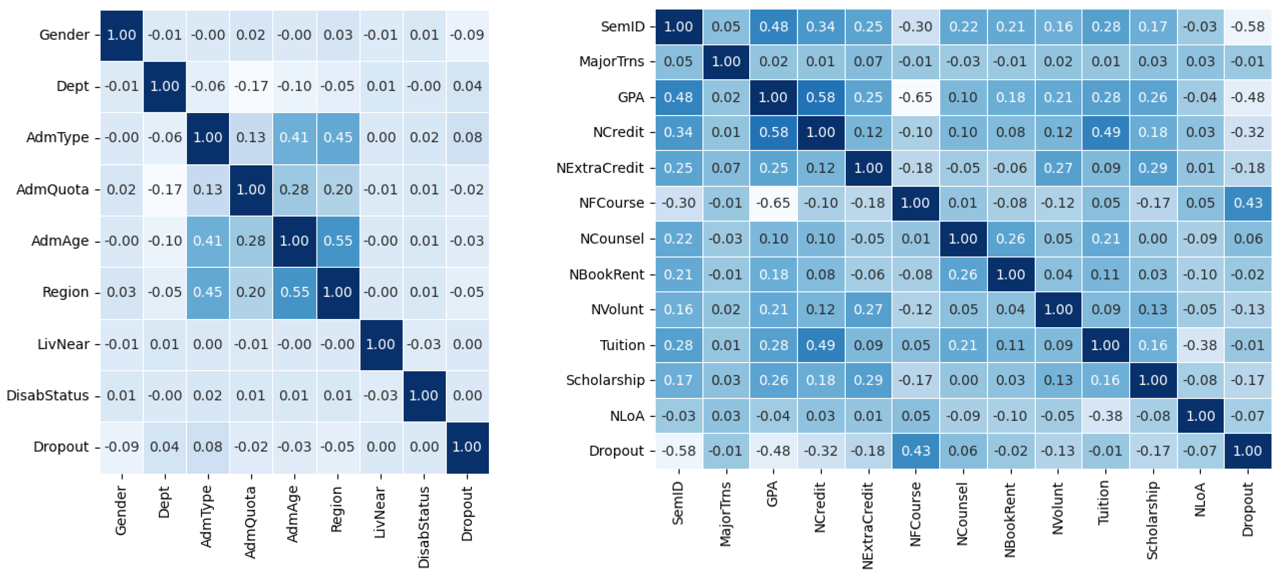
Figure 1 shows the correlation coefficients with Dropout for each attribute in Table 3 and Table 4. The attributes in Table 4 showed higher correlation coefficients than the attributes in Table 3. Some of the attributes, such as LivNear and DisabStatus, had no correlation with Dropout. SID was not considered because it is only used to link records in the two tables and is not meaningful in learning.

To select attributes used for learning, we checked various combinations of hyperparameters of a model and thresholds for correlation coefficients. As will be discussed in Section 4, we obtained the best performance when the threshold was set to 0.01. As a result, the attributes used for learning in the proposed method were summarized in

Table 7. Attributes used for learning in the proposed method.

Category	Attributes
Affiliation information	Gender, Dept, AdmType, AdmQuota, AdmAge, Region
Academic achievement information	SemID, MajorTrns, GPA, NCredit, NExtraCredit, NFCourse, NCounsel, NBookRent, NVolunt, Tuition, Scholarship, NLoA

. A total of 6 and 12 attributes were used, which represent students’ affiliation and academic achievement information, respectively.

Figure 1. Correlation coefficients with Dropout for each attribute in Table 3 (left) and Table 4 (right).

Figure 1. Correlation coefficients with Dropout for each attribute in Table 3 (left) and Table 4 (right).

3.3. Model Implementation

In the proposed method, RNNs were used to capture the temporal patterns in semester records. While feedforward neural networks pass information through the network, the RNN has cycles and transmits information back into itself. This enables them to extend the functionality of feedforward networks to consider previous inputs, $X_{0:t-1}$, in addition to the current input, $X_t$. The well-known RNN algorithms include the vanilla RNN, LSTM, and GRU.

The process of passing information from the previous iteration to the current step in the vanilla RNN can be described as (2) and (3). Below, the hidden state and the input at time t were represented as $H_t\in {\mathbb{R}}^{n\times h}$ and $X_t\in {\mathbb{R}}^{n\times d}$, respectively, where n is the number of samples, d is the number of attributes of each sample, and h is the number of hidden units. $W_{xh}$ and $W_{hh}$ denote the input-to-hidden and hidden-to-hidden state matrices, respectively, where $W_{xh}\in {\mathbb{R}}^{d\times h}$ and $W_{hh}\in {\mathbb{R}}^{h\times h}$. ${\sigma }_h$ denotes an activation function of the hidden state, which is usually a sigmoid or tanh (hyperbolic tangent) function. Putting all together yields (2) as the hidden variable. For simplicity, we omitted the bias parameter from the equation.

$$H_t={\sigma }_h(X_t{W}_{xh}+H_{t-1}{W}_{hh})$$

(2)

The output variable can be represented as (3). $W_{ho}\in {\mathbb{R}}^{h\times o}$ denotes a hidden-to-output state matrix, where o is the number of outputs. ${\sigma }_o$ denotes an activation function of the output state.

$$O_t={\sigma }_o\left(H_t{W}_{ho}\right)$$

(3)

As in most neural networks, vanishing gradients are a key problem of the RNN [45]. As the input sequence becomes longer, the performance of the RNN can degrade significantly. To resolve this problem, the LSTM uses additional gates to store information that needs to be remembered for longer periods of time, including input, forget, and output gates. Using the three gates, information can be remembered or forgotten selectively. The GRU can be viewed as a simplified version of the LSTM with only two gates, including reset and update gates. It is known to be suitable when faster training is required or when dealing with smaller datasets. To simplify the discussion, equations for the gates are omitted in this paper.

To use the RNN algorithms discussed above, the shape of the input data must be the same. However, the number of semester records belonging to a student varied from 1 to 19 in our dataset. To enable learning, we make each student have eight semester records since a typical Korean university requires eight semesters of attendance to graduate. If a student has fewer than eight records, the missing records are filled in with data from the last semester in which the student participated. This is from our observation that the academic performance in the last semester in which a student attended would be an important indicator of dropout. In this way, the proposed model was designed to predict dropout not only for current students with fewer than eight records, but also for students who have already dropped out or graduated. Otherwise, if a student has more than eight records, records from the last eight semesters are selected. From this, the dimensionality of a student’s semester records can be represented as 8 × 12.

Figure 2 shows the structure of the proposed SDP model using RNN algorithms. The two RNN layers were used to capture temporal patterns in semester records while reducing the dimensionality of the data. As the RNN algorithm, the vanilla RNN, LSTM, or GRU can be used. The temporal CNN can also be used for the RNN part in the figure. Attention was used to mitigate the problem of RNNs, where accuracy can drop as input sequences become longer. As the attention mechanism, self-attention [46] and multi-head attention [47] can be used. The dimensionality of semester records was reduced from 8 × 12 to 12. This is to provide a fair comparison with existing methods that convert a list of values for each attribute into a single summary value, such as a mean.

Figure 3 shows an example code to process semester records, where the vanilla RNN and self-attention were used for the RNN and attention mechanisms, respectively. For implementation, Keras [48], an open-source library provided by Google, was used. The SimpleRNN class represents the vanilla RNN in Keras, and it can be substituted with the LSTM or GRU class. It can also be replaced by TCN, an external class provided by the Keras Temporal Convolutional Network project [49], to implement the temporal CNN.

The first parameter of SimpleRNN in Figure 3 represents the number of hidden units or neurons in the layer, which determines the dimensionality of the output space. The return_sequences parameter was set to True to force the layer to output the hidden state for each time step. This makes the output dimension of the first RNN layer 8 × 128. The output is passed to the self-attention layer. For implementation, the external SeqSelfAttention class was used, which was provided by the Keras Self-Attention project [50]. It can be replaced by the MultiHeadAttention class provided by Keras to implement multi-head attention. The output dimension of the attention layer is the same as the input dimension. The second SimpleRNN layer was defined without the return_sequences parameter. In this case, the layer outputs only the hidden state of the last time step. From this, the dimensionality of the data is reduced from 8 × 128 to 12.

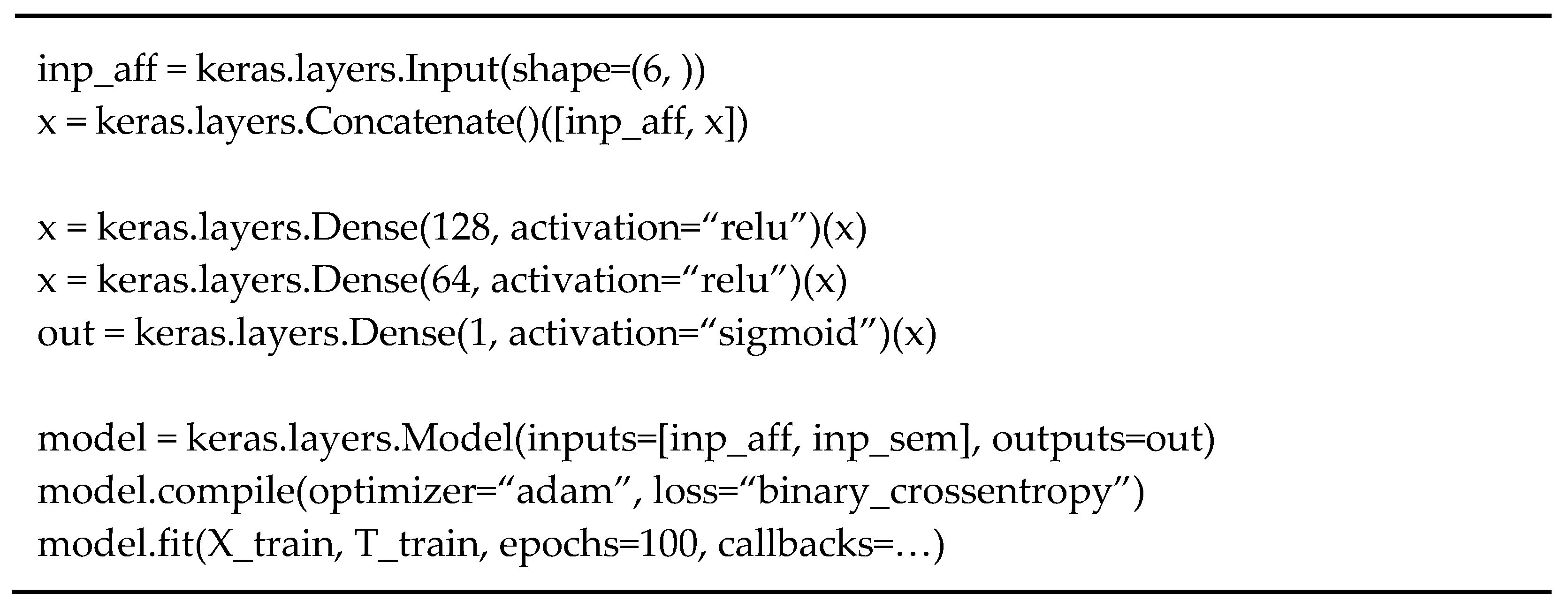
The reduced semester data is then concatenated to the affiliation data, which is a six-dimensional vector. The concatenated vector is input into fully connected layers for classification. Figure 4 shows the implementation code of a model to determine whether the concatenated vector is from a dropout student. The first two lines concatenate two vectors of a student’s affiliation data and reduced semester records. The concatenated vector is passed to fully connected layers, denoted as Dense layers. The Dense layer has two parameters to specify the number of hidden nodes and the activation function. As the activation function, the ReLU (Rectified Linear Unit) function was used in the first two hidden layers for output calculation, and the sigmoid function was used in the last layer for binary classification. Adam [51] was used as an optimizer, and the binary_crossentropy was used as a loss function. The training was set to be performed up to 100 epochs, but it could be stopped earlier by applying callbacks. X_train represents the training dataset containing all attributes except Dropout, while T_train only has class labels in Dropout. The ratio of the training and test datasets was 8:2. Thus, out of the total 20,285 records, 16,228 records were used to train the model, and the remaining 4057 records were used to validate the model’s prediction performance.

Note that the structure of the fully connected model shown in Figure 4 was determined from the repeated experiments to obtain the best prediction performance. To determine the structure, we tested various combinations of hyperparameter settings, which will be discussed in Section 4.3.

Table 8. Hyperparameter settings used to implement the proposed SDP models.

Algorithm	Parameters		Description	Value
SimpleRNN, LSTM, GRU, and TCN	Layer-1	units	Dimensionality of the output space	128
		return_sequences	Whether to return the hidden state output for each time step of the input sequence	True
	Layer-2	units	Dimensionality of the output space	12
SeqSelfAttention	Layer-1	attention_activation	Activation function to calculate output for the next layer	sigmoid
MultiHeadAttention	Layer-1	num_heads	Number of attention heads	4
		key_dim	Size of each attention head for query and key	32
ANN	Layer-1	units	Dimensionality of the output space	128
		activation	Activation function to calculate output for the next layer	relu
	Layer-2	units	Dimensionality of the output space	32
		activation	Activation function to calculate output for the next layer	relu
	Layer-3	units	Dimensionality of the output space	1
		activation	Activation function to calculate output for the next layer	sigmoid

summarizes hyperparameter settings used to implement the proposed SDP model, which was obtained from the experiments. The batch size and the learning rate were 32 and 0.001, respectively.

To improve the performance of the proposed SDP model, two additional techniques can be applied. The first is oversampling. As discussed in Section 3.1, our dataset is imbalanced, with a dropout rate of 15.2%. To address data imbalance and achieve performance improvement, oversampling techniques such as the synthetic minority oversampling technique (SMOTE) [52] and the adaptive synthetic sampling approach (ADASYN) [53] can be applied. The second is masking. To make input sequences have an equal size (i.e., 8 × 12), padding was applied by default in the proposed method. For example, if a student has fewer than eight semester records, missing records are filled in with data from the last semester in which the student participated. On the other hand, it is also possible to mask the missing records with predefined patterns, such that they are not processed by the RNN algorithms. In this way, masking allows us to process input sequences dynamically rather than statistically. For the implementation, the Masking class in Keras was used; refer to [54] for implementation details. In what follows, we discuss experimental results on the performance of the proposed SDP model and the impact of the two techniques on model performance.

4. Experimental Results

4.1. Performance Measure

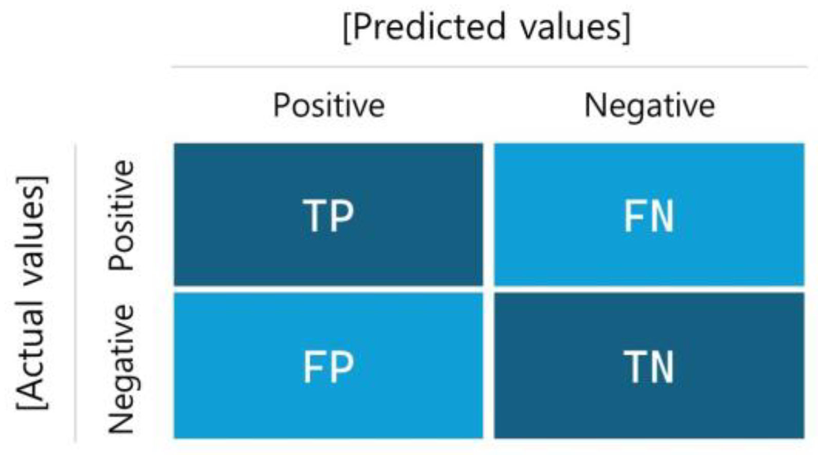
SDP is a binary classification problem, where dropout samples are generally classified into the P (Positive) class, while non-dropout samples are classified into the N (Negative) class. To determine the prediction performance, the confusion matrix shown in Figure 5 is used. In SDP, TP (True Positive) refers to the number of cases where the model correctly predicts student dropout, while FP (False Positive) refers to the number of cases where the model incorrectly predicts the dropout. TN (True Negative) and FN (False Negative) can be interpreted in the same way.

The most common measure to evaluate the prediction performance is accuracy, which can be defined as the number of classes correctly predicted by the model divided by the total number of predictions.

$$Accuracy={\displaystyle \frac{TP+TN}{TP+FP+FN+TN}}$$

(4)

The accuracy may not be properly used when the data are skewed to one class. For example, the dropout rate of four-year universities in the Republic of Korea is about 5% [11,37], where the data are highly skewed to the N class. In this case, simply predicting that no one will drop out would yield 95% accuracy. If the opposite prediction is made, the accuracy significantly drops to 5%. This example shows that FP and FN should be considered together when measuring the prediction performance. Precision can be used to measure the performance from the perspective of FP and is defined as follows:

$$Precision={\displaystyle \frac{TP}{TP+FP}}$$

(5)

Similarly, recall can be used to measure the performance from the perspective of FN, which is defined as follows:

$$Recall={\displaystyle \frac{TP}{TP+FN}}$$

(6)

A simple way to measure the performance considering both FP and FN is to use the average of precision and recall. The F1-score is defined as the harmonic mean of precision and recall.

$$F1=2\times {\displaystyle \frac{Precision\times Recall}{Precision+Recall}}$$

(7)

In this paper, the F1-score was used to evaluate the performance of prediction models since it can properly reflect the data imbalance in the performance evaluation.

4.2. Experimental Setup

4.2.1. Configuration for Existing Models

In the existing summary-based approaches, summaries can be obtained from multivalued attributes in the semester records using the following three methods, which were discussed in [11,12]:

(1)

Last semester: choose the value of the last semester as the summary.

(2)

Mean: choose the arithmetic mean of the list values as the summary.

(3)

Weighted mean: choose the weighted mean as the summary, which gives higher weight to recent semesters. The simple exponential smoothing function [50] can be used to calculate the weighted mean, such that the following applies:

$$y=\alpha y_t+\alpha \left(1-\alpha \right)y_{t-1}+\alpha {\left(1-\alpha \right)}^2{y}_{t-2}+\cdots$$

where $\alpha$ is a weight and $y_t$ is the value of the most recent semester. In the experiment, $\alpha$ was set to 0.75.

To evaluate the performance of each method, the ANN model shown in Figure 4 was adopted in the experiments.

In addition, the CNN model was adopted to check whether there are spatial patterns in the students’ semester records, as discussed in [43,44]. Figure 6 shows the structure of the experimental CNN model. In the model, the dimensionality of semester records was reduced from 8 × 12 to 12, which is the same as in the proposed SDP model shown in Figure 2.

Figure 7 shows the Keras code to implement the dimensionality reduction of the semester records. Semester records are first fed into the 2D convolutional layer, where sixteen 3 × 3 kernels are used to extract spatial patterns of the input data. To facilitate the calculation of the output size, zero-padding was applied to the data; hence, the output matrix has the shape of 8 × 12 × 16, where 16 is the number of kernels. To implement zero-padding, the padding parameter was set to “same” in the above code. The output matrix is then reduced to half its size through the max-pooling layer with a 2 × 2 kernel. But the output from the max-pooling layer is still larger than the target size, 12. Therefore, we applied another convolutional and pooling layer with the same parameters. As a result, the size of the output matrix becomes 2 × 3 × 2, which can be converted to a 12-dimensional vector by flattening. The remaining code to implement data concatenation and fully connected layers is identical to Figure 4.

4.2.2. Performance Validation

To obtain reliable performance measurements, five-fold cross-validation was conducted for each experimental model. To secure robustness across folds, the cross-validation was performed six times. From this, model performance was calculated as an average of 30 measurements.

Figure 8 shows the process of the five-fold cross-validation. To implement it, the KFold class in scikit-learn was used. The input data with 20,285 records is first divided into five equal-sized folds or subsets. For the split data, iterative training and testing are performed. In each iteration, one of the five folds is designated as the test dataset. The remaining four folds are used to train the model. For the training dataset, oversampling is applied to address data imbalance. The model is then trained with the oversampled training dataset. After the training, the performance of the model is evaluated on the test dataset. After the iteration is finished, another fold is designated as the test dataset, and the training and testing are performed for the new datasets. After all folds are evaluated on the test dataset, the average of the five F1 scores is obtained and provided as the final performance of the model.

As experimental data, 150,720 semester records collected from 20,285 students in a four-year university in Seoul, Republic of Korea, were used. The dropout rate was approximately 15.2% in the data. The experiments were conducted using Google Colab with Python 3.8, TensorFlow 2.3.0, and Keras 2.4.3. The models were tested using a system that has a V100 GPU and 40 GB of memory.

4.3. Performance Evaluation

4.3.1. Determination of the Correlation Coefficient Threshold

We first examined the impact of the correlation coefficient threshold on prediction performance. To calculate correlation coefficients, the mean-based summarization was used for semester records, which was discussed in Section 3.2. For the experiment, various forms of ANN models were used, each of which was simply a stack of fully connected layers, as shown in Figure 4.

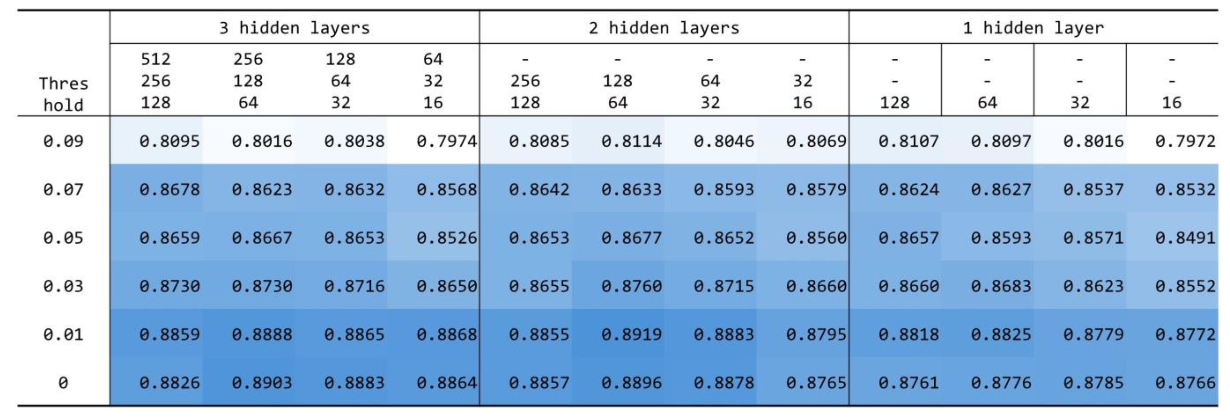
Figure 9 shows the F1 scores of the experimental models according to the correlation coefficient threshold and hidden layer configuration, where the underlined score denotes the highest score. The number in a column header of the table indicates the number of hidden units or neurons in the hidden layer. For example, the column header “(512 256 128) in three hidden layers” indicates a model consisting of three sequentially connected hidden (Dense) layers with 512, 256, and 128 nodes, respectively. The model consisting of two hidden layers with 128 and 64 nodes, when the threshold was set to 0.01, showed the best performance with an F1 score of 0.8919. We also tested using more hidden layers, but the performance was similar or worse as the number of layers increased.

Figure 10 shows the average F1 scores of the experimental models according to the correlation coefficient threshold. When the threshold was set to 0.01, the average score was the best, with an F1 score of 0.8844. From this, the threshold for feature selection was set to 0.01 in the proposed method, as discussed in Section 3.2.

Figure 11 shows the average F1 scores of the experimental models according to the hidden layer configuration. When the two hidden layers with 128 and 64 nodes were used, the average score was the best, with an F1 score of 0.8666. From this, the two hidden layers were adopted for classification in the proposed method, as shown in Figure 4. The same configuration was also adopted for the ANN model to examine the performance of the existing summary-based approaches.

4.3.2. Performance of the Basic RNNs

We then examined the performance of the basic SDP models without attention, including the vanilla RNN, LSTM, GRU, and TCN.

Figure 12 compares the performance of the four models with the existing mean-based summarization model, where the vanilla RNN and existing models are denoted as SimRNN and ANN, respectively. Among the models, GRU performed the best, with an F1 score of 0.9398. In terms of precision, the four models, except TCN, provided similar performance. In terms of recall, the models, except the ANN model, were similar. The F1 scores of the models were more affected by recall than by precision. For example, GRU had the highest F1 score and recall, while ANN had the lowest F1 score and recall. Note that all the basic SDP models, including SimRNN, LSTM, GRU, and TCN, presented better performance than the existing model, indicating that the algorithms utilized temporal patterns in the data. Especially, RNN variants including SimRNN, LSTM, and GRU improved the F1 score by at least 3%, demonstrating the effectiveness of the proposed method.

Figure 13 compares AUC-ROC (Area Under the Curve—Receiver Operating Characteristic) and AUC-PR (Area Under the Curve—Precision and Recall) for the basic SDP models. Since five-fold cross-validation was used for model evaluation, the curves were obtained using the macro-averages of the true-positive rate (TPR) and false-positive rate (FPR) values from the five folds. As a result, AUC-ROC and AUC-PR of all models were higher than 0.96, indicating that the models provide highly reliable classification performance. Among the models, GRU provided the best performance with AUC-ROC and AUC-PR of 0.990 and 0.971, respectively.

We also tested robustness across folds in our experiments. Figure 14 shows the means and standard deviations of 30 performance measurements of the basic SDP models. The standard deviations of all models were lower than 0.015, showing that model performance was consistent across folds with small variance.

4.3.3. Influence of Attention Mechanisms

We then examined the efficacy of attention mechanisms in the proposed SDP model. Figure 15 compares the performance of Simple RNN, LSTM, GRU, and TCN before and after applying self-attention and multi-head attention. Note that the attention did not necessarily help improve the performance of all models. The performance of LSTM and TCN was improved, while the performance of SimRNN and GRU, which have relatively simpler structures than LSTM and TCN, was not.

We also investigated the influence of input sequence masking on the performance of models with attention mechanisms. Figure 16 compares the performance of the 12 models after masking was applied to the input sequence, i.e., students’ semester records. The result showed that the masking degraded the performance of all self-attention models, while the performance of LSTM and TCN with multi-head attention was improved compared to the models without attention. Especially, the LSTM model with multi-head attention showed the best performance thus far, with an F1 score of 0.9401.

4.3.4. Influence of Oversampling

The student dataset is imbalanced since the dropout rate is approximately 15.2%. To address data skewness and achieve better performance, oversampling techniques such as SMOTE and ADASYN can be applied. We investigated the influence of oversampling on the performance of the proposed SDP models. To oversample and balance the training dataset, SMOTE was adopted.

Figure 17 compares the F1 scores of the proposed SDP models before and after applying SMOTE. In the figure, MHA denotes multi-head attention with input sequence masking. Self-attention models and multi-head attention models without masking were not compared in the figure because their performance was lower than that of the basic SDP models. The performance of the basic SDP models degraded after applying SMOTE. For example, the average F1 score of the models was 0.9295, but after oversampling, the score dropped to 0.9282. This was due to the fact that both average precision and recall of the models dropped from 0.9407 and 0.9383 to 0.9245 and 0.9137, respectively. On the other hand, for the models with multi-head attention, the average score improved from 0.9313 to 0.9330. This is because the average recall of the models improved from 0.9222 to 0.9309, but the average precision did not drop relatively much from 0.9409 to 0.9358.

Especially, the GRU model with multi-head attention achieved the best performance, with an F1 score of 0.9416, after applying SMOTE. The AUC-ROC and AUC-PR of the model were 0.9878 and 0.9711, respectively. The ROC and PR curves were similar to those in Figure 13. The standard deviation of the scores obtained from 30 measurements was 0.010, showing that the results are stable.

4.3.5. Spatial Temporality in Semester Records

We also investigated the performance of the CNN model discussed in Section 4.2.1 to determine whether there are spatial patterns in the students’ semester records, as well as temporal patterns. Figure 18 compares the prediction performance of the CNN model with the GRU + MHA model, which is the best-performing model among the proposed SDP models, and the existing ANN model using the mean-based summarization. Note that the F1 score of the CNN model was similar to or slightly lower than that of the existing ANN model. The result shows that it remains unclear whether spatial patterns exist in semester records.

5. Conclusions

In this paper, we tried to identify the patterns in the students’ semester records and find machine-learning algorithms that can provide satisfactory performance on the data. For this purpose, various machine-learning algorithms, including ANN, CNN, vanilla RNN, LSTM, GRU, and Temporal CNN (TCN), were compared. Attention mechanisms, including self-attention and multi-head attention, were also adopted to further improve model performance. For the experiments, 150,720 academic records collected from 20,285 students in a four-year university in Seoul, Republic of Korea, were used. The results showed that RNN variants and TCN provided better performance than other algorithms, indicating that semester records exhibit temporal patterns. The best performing model was GRU with multi-head attention, with an F1 score of 0.9416, which was approximately 5% higher than the F1 score of 0.8919 of the conventional mean-based approaches. We also conducted experiments using a CNN model to determine whether spatial patterns exist in semester records, but did not obtain meaningful results in this regard.

Through this case study, we provided evidence that semester records exhibit temporal patterns. However, this study has a clear limitation in that the proposed method was validated on only one dataset, and therefore, the findings of this study could not be generalized to other university data. But we would like to emphasize that the issue of the lack of generalizability can be mitigated through the in-depth analysis using various experiments conducted in this study. To secure our findings, further experiments using more university datasets will be conducted in the future. We also plan to study and develop more advanced models utilizing transformers that can be configured dynamically using various types of encoders and decoders. The transformer–RNN hybrid can be an option to achieve better performance. Furthermore, as discussed in the MOOC studies, we will research an evolving model that can predict student dropout on a semester-by-semester basis and support early detection of the dropout.

References

1. Kim, D.; Kim, S. Sustainable education: Analyzing the determinants of university student dropout by nonlinear panel data models. Sustainability 2018, 10, 954. [Google Scholar] [CrossRef]
2. Mduma, N.; Kalegele, K.; Machuve, D. A survey of machine learning approaches and techniques for student dropout prediction. Data Sci. J. 2019, 18, 14. [Google Scholar] [CrossRef]
3. Fierro Saltos, W.R.; Fierro Saltos, F.E.; Elizabeth Alexandra, V.S.; Rivera Guzmán, E.F. Leveraging Artificial Intelligence for Sustainable Tutoring and Dropout Prevention in Higher Education: A Scoping Review on Digital Transformation. Information 2025, 16, 819. [Google Scholar] [CrossRef]
4. Pelima, L.R.; Sukmana, Y.; Rosmansyah, Y. Predicting university student graduation using academic performance and machine learning—A systematic literature review. IEEE Access 2024, 12, 23451–23465. [Google Scholar] [CrossRef]
5. Alnasyan, B.; Basheri, M.; Alassafi, M. The power of deep learning techniques for predicting student performance in virtual learning environments: A systematic literature review. Comput. Educ. Artif. Intell. 2024, 6, 100231. [Google Scholar] [CrossRef]
6. Colpo, M.P.; Primo, T.T.; Aguiar, M.S.; Cechinel, C. Educational data mining for dropout prediction: Trends, opportunities, and challenges. Rev. Bras. Inform. Educ. 2024, 32, 220–256. [Google Scholar] [CrossRef]
7. Prenkaj, B.; Velardi, P.; Stilo, G.; Distante, D.; Faralli, S. A survey of machine learning approaches for student dropout prediction in online courses. ACM Comput. Surv. 2020, 53, 1–34. [Google Scholar] [CrossRef]
8. Alyahyan, E.; Dustegor, D. Predicting academic success in higher education: Literature review and best practices. Int. J. Educ. Technol. High. Educ. 2020, 17, 3. [Google Scholar] [CrossRef]
9. Oriveira, C.F.; Sobral, S.R.; Ferreira, M.J.; Moreira, F. How does learning analytics contribute to prevent students’ dropout in higher education: A systematic literature review. Big Data Cogn. Comput. 2021, 5, 64. [Google Scholar] [CrossRef]
10. Mbunge, E.; Batani, J.; Mafumbate, R.; Gurajena, C.; Fashoto, S.; Rugube, T.; Akinnuwesi, B.; Metfula, A. Predicting student dropout in massive open online courses using deep learning models-A systematic review. In Cybernetics Perspectives in Systems. CSOC 2022. Lecture Notes in Networks and Systems; Springer: Cham, Switzerland, 2022; pp. 212–231. [Google Scholar] [CrossRef]
11. Song, Z.; Sung, S.H.; Park, D.M.; Park, B.K. All-year dropout prediction modeling and analysis for university students. Appl. Sci. 2023, 13, 1143. [Google Scholar] [CrossRef]
12. Cho, C.H.; Yu, Y.W.; Kim, H.G. A study on dropout prediction for university students using machine learning. Appl. Sci. 2023, 13, 12004. [Google Scholar] [CrossRef]
13. Mubarak, A.A.; Cao, H.; Hezam, I.M. Deep analytic model for student dropout prediction in massive open online courses. Comput. Electr. Eng. 2021, 93, 107271. [Google Scholar] [CrossRef]
14. Tang, X.; Zhang, H.; Zhang, N.; Yan, H. Dropout rate prediction of massive open online courses based on convolutional neural networks and long short-Term memory metwork. Mob. Inf. Syst. 2022, 2022, 1–11. [Google Scholar] [CrossRef]
15. Talebi, K.; Torabi, Z.; Daneshpour, N. Ensemble models based on CNN and LSTM for dropout prediction in MOOC. Expert. Syst. Appl. 2024, 235, 121187. [Google Scholar] [CrossRef]
16. Pelletier, C.; Webb, G.I.; Petitjean, F. Temporal convolutional neural network for the classification of satellite image time series. Remote Sens. 2019, 11, 523. [Google Scholar] [CrossRef]
17. Yadav, S.P.; Zaidi, S.; Mishra, A.; Yadav, V. Survey on machine learning in speech emotion recognition and vision systems using a recurrent neural network (RNN). Arch. Comput. Methods Eng. 2022, 29, 1753–1770. [Google Scholar] [CrossRef]
18. Yu, Y.; Si, X.; Hu, C.; Zhang, J. A review of recurrent neural networks: LSTM cells and network architectures. Neural Comput. 2019, 31, 1235–1270. [Google Scholar] [CrossRef]
19. Chung, J.; Gulcehre, C.; Cho, K.; Bengio, Y. Empirical evaluation of gated recurrent neural networks on sequence modeling. arXiv 2014, arXiv:1412.3555. [Google Scholar] [CrossRef]
20. Vaswani, A.; Shazeer, N.; Parmar, N.; Uszkoreit, J.; Jones, L.; Gomez, A.N.; Kaiser, Ł.; Polosukhin, I. Attention is all you need. In Proceedings of the 31st Conference on Neural Information Processing Systems (NIPS 2017), Long Beach, CA, USA, 4–9 December 2017. [Google Scholar]
21. KDDCup2015, Biendata. Available online: https://www.biendata.xyz/competition/kddcup2015/rank/ (accessed on 21 August 2025).
22. OULAD, Open University Learning Analytics Dataset, UC Irvine Machine Learning Repository. Available online: https://archive.ics.uci.edu/dataset/349/open+university+learning+analytics+dataset (accessed on 21 August 2025).
23. Li, Z.; Liu, F.; Yang, W.; Peng, S.; Zhou, J. A survey of convolutional neural networks: Analysis, applications, and prospects. IEEE Trans. Neural Netw. Learn. Syst. 2021, 33, 6999–7019. [Google Scholar] [CrossRef]
24. Zheng, Y.; Gao, Z.; Wang, Y.; Fu, Q. MOOC dropout prediction using FWTS-CNN model based on fused feature weighting and time series. IEEE Access 2020, 8, 225324–225335. [Google Scholar] [CrossRef]
25. Wen, Y.; Tian, Y.; Wen, B.; Zhou, Q.; Cai, G.; Liu, S. Consideration of the local correlation of learning behaviors to predict dropouts from MOOCs. Tsinghua Sci. Technol. 2019, 25, 336–347. [Google Scholar] [CrossRef]
26. Feng, W.; Tang, J.; Liu, T.X. Understanding dropouts in MOOCs. In Proceedings of the AAAI Conference on Artificial Intelligence, Honolulu, HI, USA, 27 January–1 February 2019; 33, pp. 517–524. [Google Scholar] [CrossRef]
27. Pan, F.; Huang, B.; Zhang, C.; Zhu, X.; Wu, Z.; Zhang, M.; Ji, Y.; Ma, Z.; Li, Z. A survival analysis based volatility and sparsity modeling network for student dropout prediction. PLoS ONE 2022, 17, e0267138. [Google Scholar] [CrossRef]
28. Niu, K.; Lu, G.; Peng, X.; Zhou, Y.; Zeng, J.; Zhang, K. CNN autoencoders and LSTM-based reduced order model for student dropout prediction. Neural Comput. Appl. 2023, 35, 22341–22357. [Google Scholar] [CrossRef]
29. Kumar, G.; Singh, A.; Sharma, A. Ensemble deep learning network model for dropout prediction in MOOCs. Int. J. Electr. Comput. Eng. Syst. 2023, 14, 187–196. [Google Scholar] [CrossRef]
30. Ren, S.; He, K.; Girshick, R.; Sun, J. Faster R-CNN: Towards real-time object detection with region proposal networks. IEEE Trans. Pattern Anal. Mach. Intell. 2016, 39, 1137–1149. [Google Scholar] [CrossRef] [PubMed]
31. Roh, D.; Han, D.; Kim, D.; Han, K.; Yi, M.Y. SIG-Net: GNN based dropout prediction in MOOCs using student interaction graph. In Proceedings of the 39th ACM/SIGAPP Symposium on Applied Computing, Ávila, Spain, 4–8 April 2024; pp. 29–37. [Google Scholar] [CrossRef]
32. Wu, Z.; Pan, S.; Chen, F.; Long, G.; Zhang, C.; Yu, P.S. A comprehensive survey on graph neural networks. IEEE Trans. Neural Netw. Learn. Syst. 2020, 32, 4–24. [Google Scholar] [CrossRef] [PubMed]
33. Waheed, H.; Hassan, S.-U.; Nawaz, R.; Aljohani, N.R.; Chen, G.; Gasevic, D. Early prediction of learners at risk in self-paced education: A neural network approach. Expert. Syst. Appl. 2023, 213, 118868. [Google Scholar] [CrossRef]
34. Mubarak, A.A.; Cao, H.; Zhang, W. Prediction of students’ early dropout based on their interaction logs in online learning environment. Interact. Learn. Environ. 2022, 30, 1414–1433. [Google Scholar] [CrossRef]
35. Kim, S.; Choi, E.; Jun, Y.K.; Lee, S. Student Dropout Prediction for University with High Precision and Recall. Appl. Sci. 2023, 13, 6275. [Google Scholar] [CrossRef]
36. Zhang, P.; Jia, Y.; Shang, Y. Research and application of XGBoost in imbalanced data. Int. J. Distrib. Sens. Net. 2022, 18, 6. [Google Scholar] [CrossRef]
37. Hancock, J.T.; Khoshgoftaar, T.M. CatBoost for big data: An interdisciplinary review. J. Big Data 2020, 7, 94. [Google Scholar] [CrossRef]
38. Zanellati, A.; Zingaro, S.P.; Gabbrielli, M. Balancing performance and explainability in academic dropout prediction. IEEE Trans. Learn. Tech. 2024, 17, 2086–2099. [Google Scholar] [CrossRef]
39. Ujkani, B.; Minkovska, D.; Stoyanova, L. Application of logistic regression technique for predicting student dropout. In Proceedings of the 2022 XXXI International Scientific Conference Electronics (ET), Sozopol, Bulgaria, 13–15 September 2022; pp. 1–4. [Google Scholar] [CrossRef]
40. Rabelo, A.M.; Zárate, L.E. A model for predicting dropout of higher education students. Data Sci. Manag. 2025, 8, 72–85. [Google Scholar] [CrossRef]
41. Nieto, Y.; Gacía-Díaz, V.; Montenegro, C.; González, C.C.; Crespo, R.G. Usage of machine learning for strategic decision making at higher educational institutions. IEEE Access 2019, 7, 75007–75017. [Google Scholar] [CrossRef]
42. Ke, G.; Meng, Q.; Finley, T.; Wang, T.; Chen, W.; Ma, W.; Ye, Q.; Liu, T.-Y. Lightgbm: A highly efficient gradient boosting decision tree. In Proceedings of the 31st International Conference on Neural Information Processing Systems (NIPS’17), Long Beach, CA, USA, 4–9 December 2017; Volume 30. [Google Scholar]
43. Agrusti, F.; Mezzini, M.; Bonavolontà, G. Deep learning approach for predicting university dropout: A case study at Roma Tre University. J. E-Learn. Knowl. Soc. 2020, 16, 44–54. [Google Scholar] [CrossRef]
44. Gutierrez-Pachas, A.; Garcia-Zanabria, G.; Cuadros-Vargas, E.; Camara-Chavez, G.; Gomez-Nieto, E. Supporting decision-making process on higher education dropout by analyzing academic, socioeconomic, and equity factors through machine learning and survival analysis methods in the Latin American context. Edu. Sci. 2023, 13, 154. [Google Scholar] [CrossRef]
45. Rehmer, A.; Kroll, A. On the vanishing and exploding gradient problem in gated recurrent units. IFAC-PapersOnLine 2020, 53, 1243–1248. [Google Scholar] [CrossRef]
46. Shaw, P.; Uszkoreit, J.; Vaswani, A. Self-attention with relative position representations. arXiv 2018, arXiv:1803.02155. [Google Scholar] [CrossRef]
47. Cordonnier, J.B.; Loukas, A.; Jaggi, M. Multi-head attention: Collaborate instead of concatenate. arXiv 2020, arXiv:2006.16362. [Google Scholar] [CrossRef]
48. Keras, Google. Available online: https://keras.io/ (accessed on 21 August 2025).
49. Keras Self-Attention Project, Google. Available online: https://pypi.org/project/keras-self-attention/ (accessed on 21 August 2025).
50. Keras Temporal Convolutional Network Project, Google. Available online: https://pypi.org/project/keras-tcn/2.9.3/ (accessed on 15 October 2025).
51. Adam, K.D.B.J. A method for stochastic optimization. arXiv 2014, arXiv:1412.6980. [Google Scholar] [CrossRef]
52. Chawla, N.V.; Bowyer, K.W.; Hall, L.O.; Kegelmeyer, W.P. SMOTE: Synthetic minority over-sampling technique. J. Artif. Intell. Res. 2002, 16, 321–357. [Google Scholar] [CrossRef]
53. Alhudhaif, A. A novel multi-class imbalanced EEG signals classification based on the adaptive synthetic sampling (ADASYN) approach. PeerJ Comput. Sci. 2021, 7, e523. [Google Scholar] [CrossRef] [PubMed]
54. Keras Masking and Padding, Google. Available online: https://www.tensorflow.org/guide/keras/understanding_masking_and_padding?hl=en (accessed on 15 October 2025).
Figure 2. Structure of the proposed SDP model using RNN algorithms with attention.
Electronics 14 04356 g002
Figure 3. Keras code to process semester records using SimpleRNN and SeqSelfAttention.
Electronics 14 04356 g003
Figure 4. Keras code to build the SDP model with data concatenation and fully connected layers for classification.
Electronics 14 04356 g004
Figure 5. A confusion matrix to evaluate the performance of a binary classification model.
Electronics 14 04356 g005
Figure 6. Structure of the CNN model to process students’ affiliation and semester records.
Electronics 14 04356 g006
Figure 7. Keras code to process semester records using Conv2D and MaxPooling2D.
Electronics 14 04356 g007
Figure 8. Five-fold cross-validation process to measure the performance of each experimental model.
Electronics 14 04356 g008
Figure 9. F1 scores of the experimental models according to the correlation coefficient threshold and hidden layer configuration.
Electronics 14 04356 g009
Figure 10. Average F1 scores of the experimental models according to the correlation coefficient threshold.
Electronics 14 04356 g010
Figure 11. Average F1 scores of the experimental models according to the hidden layer configuration.
Electronics 14 04356 g011
Figure 12. F1 scores, precision, and recall of the existing model (denoted as ANN) and basic SDP models without attention (denoted as SimRNN, LSTM, GRU, and TCN, respectively).
Electronics 14 04356 g012
Figure 13. Macro-average AUC-ROC and AUC-PR for the basic SDP models.
Electronics 14 04356 g013
Figure 14. Mean and standard deviation of 30 performance measurements of the basic SDP models.
Electronics 14 04356 g014
Figure 15. F1 scores of the basic SDP models before and after applying attention mechanisms.
Electronics 14 04356 g015
Figure 16. F1 scores of the basic SDP models after the masking was applied to input sequences.
Electronics 14 04356 g016
Figure 17. Comparisons of the F1 scores of the basic SDP models and the models with multi-head attention (denoted as SimRNN + MHA, LSTM + MHA, GRU + MHA, and TCN + MHA) before and after applying SMOTE.
Electronics 14 04356 g017
Figure 18. Comparison of the prediction performance of the CNN model with the existing ANN model and the proposed GRU–MHA (GRU with multi-head attention) model.
Electronics 14 04356 g018