Article

Batch Cyclic Posterior Selection Particle Filter and Its Application in TRN

1
School of Internet, Anhui University, Hefei 230039, China
2
IKD New Energy Automotive Parts Company Limited, Ma’anshan 243121, China
3
Aerospace Information Research Institute, Chinese Academy of Sciences, Beijing 100094, China
4
College of Intelligent Manufacturing, Anhui Science and Technology University, Chuzhou 233199, China
*
Authors to whom correspondence should be addressed.
Electronics 2025, 14(21), 4257; https://doi.org/10.3390/electronics14214257
Submission received: 26 September 2025 / Revised: 25 October 2025 / Accepted: 28 October 2025 / Published: 30 October 2025
(This article belongs to the Special Issue Recent Advance of Auto Navigation in Indoor Scenarios)

Abstract

Terrain referenced navigation (TRN) determines position by comparing terrain height measurements with digital elevation maps (DEMs). However, terrain fluctuations create multimodal observation distributions, introducing significant nonlinearity that challenges fusion positioning algorithms. To address this, we propose a novel data fusion approach: batch cyclic posterior selection particle filter (BCPS-PF), applied to TRN. Our algorithm consists of two primary mechanisms. First, the batch cycle particle generation mechanism continuously generates particles conforming to the prior distribution. This is achieved by decomposing the state transition function and the state noise model during the prediction step. Particles from the previous time step are transformed via the state transition function, and noise sequences generated by the state noise model are added, forming batch cycle particles. Second, a particle selection mechanism filters particles to match the posterior distribution. This involves an update step in the fusion process, utilizing a rejection sampling technique. The batch cycle mechanism can be terminated by limiting the number of particles, and state estimation is derived by calculating the mean of these particles. Simulations demonstrate that our method improves positioning accuracy by over 10% compared with existing methods.

1. Introduction

Terrain referenced navigation (TRN) determines position by comparing terrain height measurements with digital elevation maps (DEMs) [1]. This method is particularly robust against electromagnetic interference and adverse weather conditions, making it suitable for applications in missiles, military aircraft, and underwater equipment [2,3,4].
Despite its advantages, TRN faces significant challenges due to the multimodal distribution of elevation observations, especially in areas with anomalous terrain profiles [5]. Traditional filtering methods often struggle to capture these complex features, leading to potential filter degeneracy and localization failure.
To address the issues associated with multimodal distributions in TRN, nonlinear filtering methods have gained increasing attention. Among these, particle filtering (PF) stands out due to its flexibility in handling nonlinear problems [6,7]. The PF models dynamic systems with nonlinear and non-Gaussian properties, making it a well-accepted estimator for TRN [8]. It implements recursive Bayesian estimation using Monte Carlo simulation to infer states from observations. The posterior probability density function (PDF) is represented by several weighted particles, with the weights calculated based on the conditional likelihood of each particle given the current observations [7,9].
However, PF encounters a unique challenge in the TRN application. The likelihood distribution presents a multimodal feature due to the undulating topography [10]. This feature does not always pose a problem; however, it will pose a serious degeneracy problem when the high probability region of the prior distribution is far away from that of the likelihood distribution [11]. This intermittent degeneracy problem greatly affects the stability of fusion localization, but this problem has not received enough attention from scholars.

1.1. Motivation

Due to the irregular terrain and sharp elevation changes, the observations provided by terrain referenced navigation (TRN) systems exhibit strong nonlinear and non-Gaussian characteristics. Therefore, researchers commonly employ sequential Monte Carlo methods (such as the particle filter (PF)) to fuse TRN observations.
However, a key challenge in achieving high-quality fusion of TRN observations—which is often overlooked in standard PF implementations—lies in ensuring that the multiple high-probability regions (modes) of the multimodal posterior distribution have sufficient non-degenerate particles to accurately represent the distribution’s characteristics. When the prior particles fall into low-likelihood regions, the traditional sequential importance resampling (SIR) PF suffers from the particle degeneracy problem, making accurate state estimation impossible.
To address this fundamental issue, we propose the batch cyclic posterior selection particle filter (BCPS-PF) algorithm. This fusion method aims to indirectly generate particles from the true posterior distribution, thereby ensuring that the high-probability regions of the posterior distribution, which play a crucial role in state estimation, have a sufficient number of high-quality particles to accurately describe their distribution characteristics.
The procedure of the BCPS-PF can be mainly divided into two parts as shown in Figure 1, directly reflecting the prediction and update steps of the Bayesian filter:
(1) Batch cyclic particle generation mechanism (prediction step). This mechanism is designed by mathematically decomposing the state transition function and the state noise model in the prediction step. Its purpose is to generate a diverse batch of proposal particles that conform to the prior distribution p x k z k 1 .
It first generates one-step transition particles based on the particles representing the posterior distribution at the previous time step using the deterministic part of the state transition function.
Subsequently, it adds a noise sequence generated from the state noise model to each one-step transition particle in a cyclic manner, thus continuously generating a large batch of proposed particles that correctly conform to the prior distribution.
(2) Posterior particle selection mechanism (update step). This mechanism is designed by integrating the Bayesian update step with the rejection sampling (RS) technique. Its purpose is to select particles that accurately conform to the posterior distribution p x k z k .
It first matches the batch cycle particles with the digital elevation map (DEM) and calculates the likelihood weights by combining the observation and observation noise model.
Then, it performs acceptance/rejection sampling on the batch cycle particles based on the magnitude of the likelihood weights. This selection mechanism effectively completes the fusion of prior and likelihood information and obtains a new particle set that statistically conforms to the posterior distribution.
Finally, we can terminate the cycle mechanism by limiting the number of accepted particles and obtain the state estimation by calculating the mean of the selected particles. This approach eliminates the explicit need for the computationally expensive and potentially biased resampling and weight propagation steps found in conventional SIR-PF.

1.2. Related Works

TRN has been widely used in the field of missiles, military aircraft, underwater equipment, and so on since the 1970s [12]. After nearly 60 years of development, TRN algorithms can be roughly divided into two categories [3,13]: one is the terrain contour matching algorithm based on a correlation analysis, such as the TERCOM [14,15]; the other is the Bayesian filtering based-inertial terrain referenced navigation algorithm, such as the Sandia inertial terrain-aided navigation (SITAN) algorithm [16,17]. With the continuous application of nonlinear filtering theory in fusion positioning technology, researchers, inspired by TERCOM and SITAN, merged these two architectures to enhance the robustness of the TRN system [18,19,20,21]. However, a measurement ambiguity problem arises in TRN when there are similar terrain profiles surrounding the aircraft, which might potentially cause filter divergence, ultimately resulting in localization failure.
Scholars have made significant efforts in improving filtering methods for addressing the issue of ambiguous measurement [2,22,23]. Linear filtering methods were widely used in the early stages [24,25]. Recently, with the advancement of computer hardware capabilities, many nonlinear filtering algorithms capable of providing better approximations to analytical solutions of Bayesian filtering (which involve slightly higher computational demands) have gradually been applied in TRN systems, achieving favorable results [26,27,28]. Refs. [6,29] treat TRN as a nonlinear filtering problem and employ point mass filtering (PMF) to overcome the linear truncation errors. Particle filtering (PF), driven by Monte Carlo methods, has the capability to describe and propagate arbitrary distributions. Therefore, it has received extensive research in TRN algorithms [30,31,32]. Ref. [33] conducts a comparative analysis of PFs with different resampling methods in TRN, and assesses their performance. Ref. [34] decomposes the linear and nonlinear components of the INS using marginal PF (MPF). It employs Kalman filtering (KF) and particle filtering (PF) for estimating the linear and nonlinear parts, respectively. This approach enhances the approximation of the analytical solution of Bayesian filtering in TRN fusion. Ref. [35] uses gradient-fitted results to correct the likelihood distribution obtained from TRN measurements in PF. Furthermore, [36] presents a new constrained cubature particle filter (CCPF) for the difficulty in nonlinear filtering. Ref. [37] adopts spherical simplex unscented transformation (SSUT) to approximate the probability distribution for achieving high accuracy. Overall, the evolution of TRN algorithms has always revolved around a central objective: approximating the analytical solution of the Bayesian method within a nonlinear filtering framework, thereby obtaining the optimal estimate in the sense of minimum mean square error (MMSE).
PF is highly suitable for addressing TRN challenges due to its flexibility in nonlinear filtering problems. However, an impoverishment problem can potentially lead to filter divergence in TRN, in situations of complex terrain or areas with multiple similar terrain features. Dealing with the issues above, the likelihood distribution associated with observations provided by the TRN may exhibit bimodal or even multimodal characteristics. The ability to fully describe such complex likelihood distribution depends on whether there are sufficient particles at each peak’s position, which is determined by the proposal distribution. When the high-probability regions of the proposal distribution do not encompass one peak of likelihood, the particles selected based on the proposal distribution are highly likely to miss the information of likelihood in this area [37]. This phenomenon can lead to filter divergence or result in incorrect position estimates within some local steps. In [38], out-of-sequence measurement (OOSM) was proposed to overcome this issue. The strategy of the proposed method is to skip the measurement update at the time step when an ambiguous measurement update is detected. This method can effectively reduce the impact of incorrect position estimates on the overall flight localization.
The difficulty of determining the shape of the likelihood distribution and the possible multimodal distribution are typical features in TRN. This feature puts forward higher requirements for the multi-source fusion algorithm. Specifically, better balance mechanisms are needed to deal with the degeneracy and impoverishment problems for the PF algorithm. It is important to note that the optimal proposal distribution is theoretically a posterior distribution, as rigorously proven in a previous work [39]. However, the actual posterior distribution is not directly accessible.

1.3. Our Contributions

This paper introduces a novel particle filter using the posterior distribution as the proposal distribution, namely the batch cyclic posterior selection particle filter (BCPS-PF), designed to address the specific challenges above. The BCPS-PF aims to improve the proposal distribution, ensuring a sufficient number of particles are in high-probability regions of the posterior distribution, enhancing accuracy. The algorithm generates batch cycle particles that adhere to the prior state distribution through state model decomposition. It then incorporates rejection sampling (RS) in the update step of the fusion process to select particles that conform to the posterior distribution, resulting in a precise state estimation. The main contributions of this paper are as follows:
(1)
Developing a mechanism to generate batch cycle particles that form cyclic continuous batches conforming to the prior distribution. This involves decomposing the state model into a state transition function and a state noise model. The state transition function transfers particles, while the state noise model ensures particle diversity, resulting in batch cycle particles that describe the prior distribution.
(2)
Designing a particle selection mechanism that integrates the update step in the fusion process with the RS technique, obtaining selected particles that conform to the posterior distribution.
(3)
Proposing the BCPS-PF algorithm, which indirectly uses the posterior distribution as the proposal distribution, avoiding the need for resampling and recursive weight transmission, thus effectively balancing degeneracy and impoverishment problems, ensuring filter accuracy and stability.
(4)
Evaluating the algorithm in inertial measurement units (IMUs) with TRN fusion positioning scenarios, demonstrating significant performance improvements.
The remainder of this paper is structured as follows: Section 2 presents the TRN principle and the fundamental concepts of data fusion. Section 3 analyzes the impact of TRN on fusion positioning during IMU/TRN fusion and introduces the motivation and framework for the BCPS-PF algorithm. Section 4 delves into the BCPS-PF, providing a detailed explanation of its two primary mechanisms: batch cycle particle generation and particle selection. Section 5 discusses the performance evaluation of the BCPS-PF in IMU/TRN fusion positioning scenarios. Finally, Section 6 concludes this paper.

2. TRN Principle and System Model

TRN utilizes digital elevation models (DEMs) to indirectly estimate the horizontal position of unmanned aerial vehicles (UAVs) by matching measured UAV height. These position estimates are then integrated with horizontal position data obtained from the IMU to enhance accuracy. This section outlines the methodology for deriving horizontal position estimates from both the IMU and TRN. Following this, we discuss the fusion localization process based on traditional PF.
IMU measures an object’s acceleration and angular velocity, typically using accelerometers and gyroscopes on three axes. Based on these measurements and an initial position, IMU can estimate a UAV’s position. This paper focuses on fusing IMU and TRN data to obtain a UAV’s horizontal position. To achieve this, we simplify the IMU mathematical model by considering only the two horizontal position parameters as the state model, as shown below:
x k = p k x , p k y T
where p k x and p k y are the position of a UAV in two directions (horizontal direction) at time step k .
The dynamic models adopted in this work are:
x k = 1 0 0 1 x k 1 + v k 1 x Δ t v k 1 y Δ t + u k 1
where v k x and v k y are real velocities corresponding to these two position directions (provided by the IMU) at time step k . u k 1 is the zero-mean Gaussian process characterizing the IMU measurement noise. Equation (2) is considered the state model.
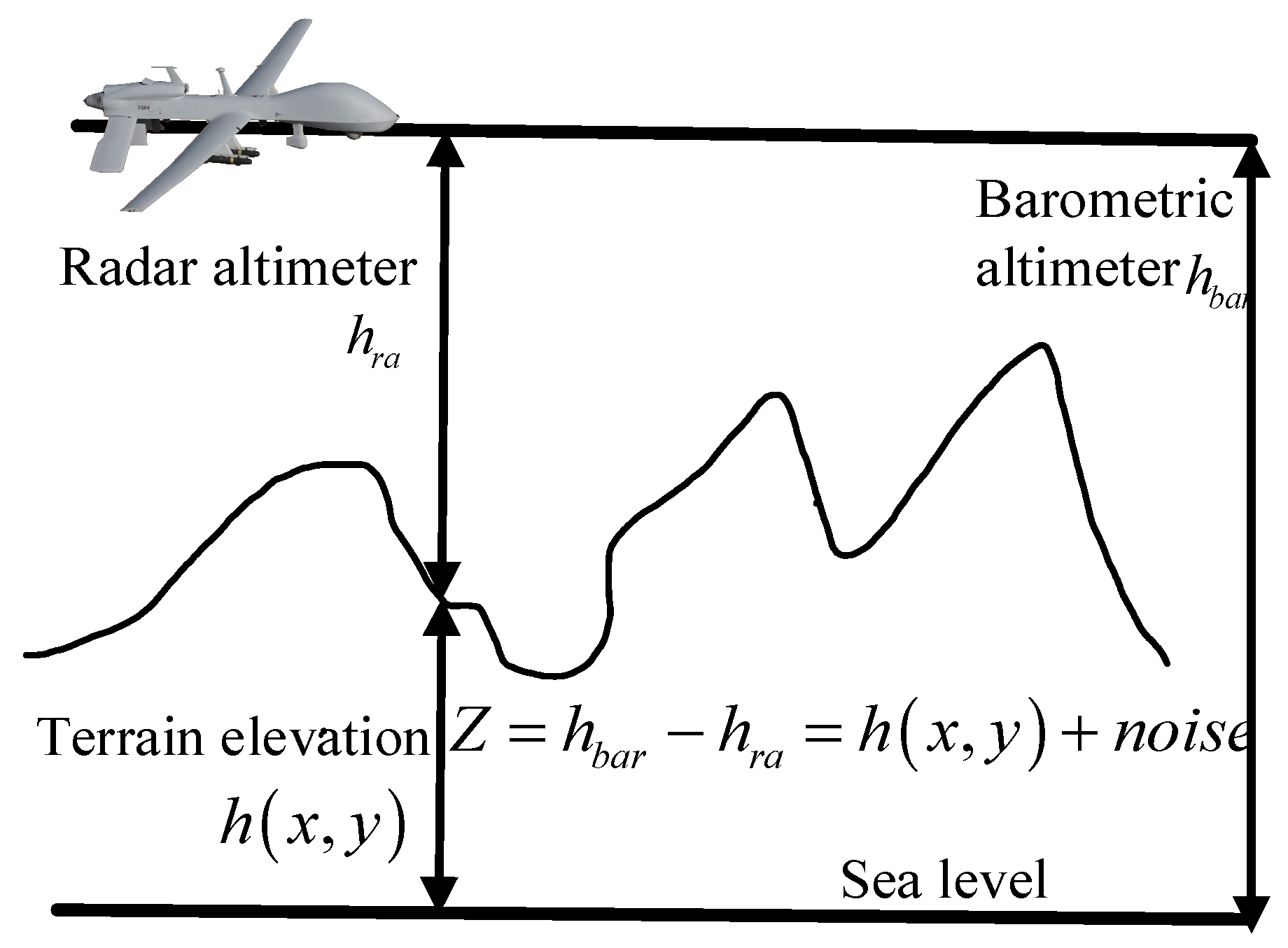
The principle of obtaining observation data by the TRN system is illustrated in Figure 2. The UAV utilizes barometer altimeter and radar altimeter to measure its current barometric altitude and radar altitude at the current position, respectively. Then, the current ground altitude at that location is obtained as an observation. In addition, this observation can be obtained by matching the current horizontal position estimated by IMU with DEM. Therefore, the dynamic measurement model characterizing the TRN system is as follows:
Z k = h x k + v k
where Z k denotes the results of the terrain elevation measurement. The real terrain elevation can be obtained from the DEM stored on the UAV. v k is a zeros-mean Gaussian processes characterizing the elevation measurement noise arising from the barometric altimeter and radar altimeter. Equation (3) is considered the observation model.

3. From Bayesian Estimation to Particle Filter

State Equation (2) can be considered as the state transition probability p x k x 0 : k 1 , whereas measurement Equation (3) represents the likelihood probability p z 0 : k x k .
The goal of the recursive Bayesian estimation is to obtain the expectation of the posterior PDF at the current time step based on Bayes’ theorem, as follows:
x ¯ k = E p x k z 1 : k
where p x k z 1 : k denotes the posterior PDF at time step k . To achieve the recursive Bayesian estimation, the filter process is usually divided into two steps: prediction and update.
Prediction: Obtaining the prior PDF using the state transition probability and the posterior probability at the last time step, as follows:
p x k z k 1 = p x k x k 1 p x k 1 z k 1 d x k 1
Update: Fusion of the prior PDF and the likelihood distribution, as follows:
p x k z k = p z k x k p x k z k 1 p z k z k 1
In this step, the fusion of the measurement is accomplished by calculating weights to particles: ω ˜ k i i = 1 N = p z k x k i i = 1 N . At this point, Equation (6) will become an integral difficulty problem due to the nonlinear characteristic in (3), which makes it impossible to obtain an analytical solution of the posterior PDF. In PF, the posterior distribution is approximated using weighted particles, as follows:
p x k z k i = 1 N ω k i δ x k x k i
where δ denotes the Dirac delta function; N denotes particle number; ω k i is the weight of the i-th particle. Although weighted samples can approximate the posterior distribution, a degeneracy problem can arise in the recursive process, leading to filter divergence. To address this issue, resampling techniques are introduced. All particles obtained through resampling have equal weights (taking SIR as an example). Therefore, Equation (7) can be rewritten as follows:
p x k z k 1 N i = 1 N δ x k x k i
A pseudo-code description of the SIR algorithm is given in Algorithm 1.
Algorithm 1. Particle filter algorithm.
Initialization:
Particle sampling is performed according to the pdf of the initial position. X 0 N ~ p x 0 and obtain observation z 1
//Overall time steps:
For k 1 to K do
(1): Draw X ^ k N p x k z k 1 according to (2), respectively;
(2): X ^ k N are matched with the DEM to generate the predicted observations z k , p r e N .
(3): Calculate the deviation ε k , p r e N = z k , p r e N z k
(4): Calculate ω ^ k N = p ε k , p r e X ^ k N , respectively;
(5): Normalization of the weights: ω k N = ω ^ k s u m ω ^ k N N , respectively;
(6): Resampling [11], and obtain X k N
(7): State estimation: x ^ k = m e a n X k N
End

4. The BCPS-PF Algorithm

4.1. Batch Cycle Particle Generation Mechanism in Prediction Step

Suppose random variable χ k 1 ~ p x k 1 z k 1 . After passing through the state model, we can obtain a new random variable χ ^ k , as shown in Figure 3. Then, χ ^ k ~ p x k z k 1 according to the prediction step [27].
While X k 1 is a set of particles that generates from χ k 1 , then the distribution characteristic of these particles can be used to represent p x k 1 z k 1 approximately. At this point, we can easily get a new set of particles X ^ k , where X ^ k = f X k 1 + u 0 and u 0 denotes the noise sequence generated by the state noise model. X ^ k is a set of particles satisfied by p x k z k 1 . When the number of particles is larger, the description of p x k 1 z k 1 by X k 1 is more accurate. At the same time, the description of p x k z k 1 by X ^ k is more accurate. However, the number of particles is always limited in a real-time PF system.
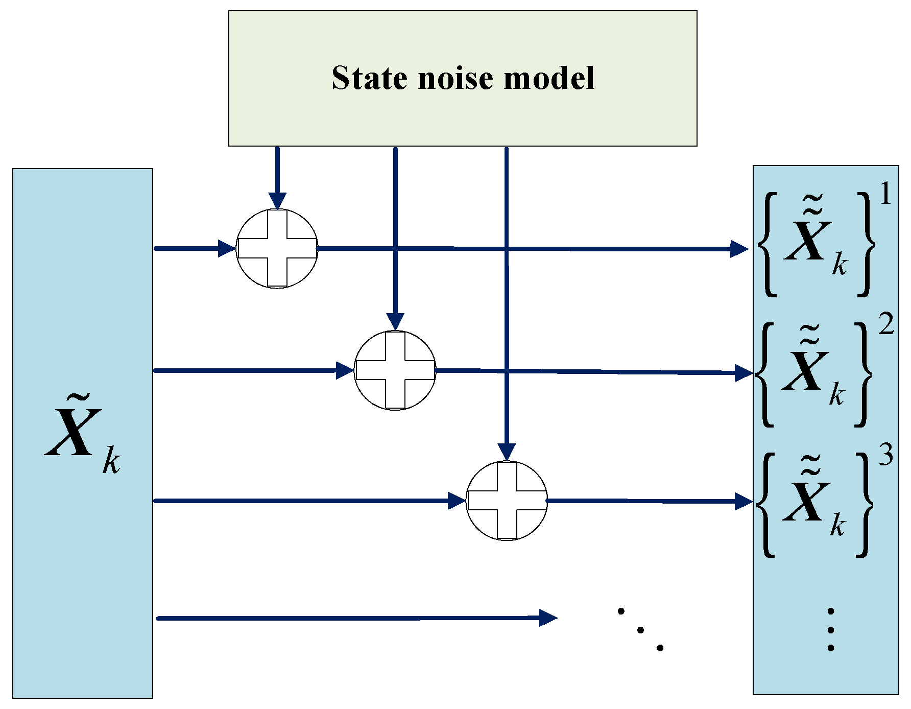
In this subsection, our goal is to obtain a particle flow that can be used to reflect p x k z k 1 as accurately as possible under the condition that the particle number of X k 1 is fixed. For this purpose, we have decomposed the state transition function with the state noise model, as shown in Figure 4. χ ˜ k is the random variable obtained by the result of the state transition function without the state noise model, called the one-step transfer random variable. p f x k 1 z k 1 is defined as the PDF of χ ˜ k , called the one-step transfer distribution. When χ ˜ k passes through the state noise model, it is defined as the PDF of χ ˜ ˜ k .
Furthermore, the one-step transfer particle X ˜ k can be used to describe p f x k 1 z k 1 , where X ˜ k = f X k 1 .
Theorem 1.
In the nonlinear system of Figure 4,  p χ ˜ k z k 1 = k 1 p χ k 1 z k 1 d χ k 1  ,where  k 1 = χ k : χ ˜ k = f χ k 1 .
Theorem 2.
In the nonlinear system of Figure 4 p χ ˜ ˜ k z k 1 = p χ ^ k z k 1  , where  p χ k z k 1  is described in Figure 3.
From Theorem 1 we can see that the random variable χ ˜ k depends on p χ k 1 z k 1 and the nonlinear system f ; from Theorem 2 we can see that the random variable χ ^ k can be used to describe the prior distribution p χ k z k 1 . When particles X k 1 N k 1 , the posteriori distribution at time step k 1 is obtained. We are able to obtain a deterministic set of particles X ˜ k N k 1 used to describe the random variable χ ˜ k due to the determinacy of nonlinear system f , where X ˜ k = f X k 1 . Consider the noise model is known, as shown in Figure 5, we can generate a particle stream X ˜ ˜ k i that represents the batch ith particle noise model and χ ˜ ˜ k ~ p x ˜ ˜ k z k 1 , where
X ˜ ˜ k i = X ˜ k + u i

4.2. Particle Selection Mechanism in Update Step

The fusion of the prior and the posterior distribution is one of the most important steps. This step is equivalent to the mathematical equation as follows:
p x k z k = p z k x k p x k z k 1 p z k z k 1
where p z k x k denotes the likelihood distribution and p x k z k 1 denotes the posterior distribution. p z k z k 1 is the normalization constant.
Compared with the batch cycle particle generation mechanism, the prediction step in the PF algorithm is equivalent to obtain X ˜ ˜ k 0 . Then the weights corresponding to particles X ˜ ˜ k 0 can be easily calculated, as follows:
ω ˜ ˜ k 0 = p z k X ˜ ˜ k 0
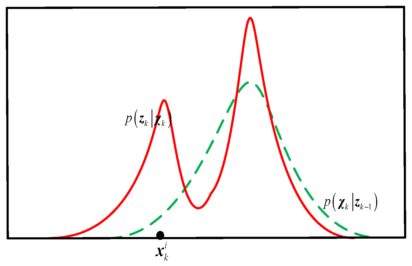
After that, the posteriori distribution can be described by the weighted particles ω ˜ ˜ k 0 , X ˜ ˜ k 0 . However, in the TRN system, when the observation exhibits a multimodal distribution, particles sampled from the proposal distribution are likely to miss certain states of the observation due to the limited number of particles, as shown in Figure 6. In this situation, part of the likelihood information can easily be lost.
In this subsection, we propose a particle selection mechanism whose core is the acceptance and rejection of weighted prior particles. This process allows us to directly acquire particles satisfying the posterior distribution and complete the state estimation.
In (5), consider p x k z k and p x k z k 1 are the target distribution and proposal distribution, respectively. We have obtained prior particles X ˜ ˜ k i in Section 4.1, which can be used to describe p x k z k 1 . According to the principle of RS construction of the acceptance probability, we can get the expression of acceptance probability as follows:
ξ < p x k z k M p x k z k 1
where ξ ~ U 0 , 1 and M is a constant used to ensure that:
M p x k z k 1 p x k z k         x k d o m p x k z k 1 d o m p x k z k
Accept the sample if the result obtained by substituting the particle into the right side of (7) is greater than a randomly generated ξ . Otherwise, reject the sample. Obtaining an explicit expression for p x k z k directly is difficult, but substitute (5) into (11), and we have:
ξ < p z k x k p x k z k 1 M p x k z k 1 p z k z k 1
Consider p z k z k 1 denotes the normalization constant and simplify (9) to get:
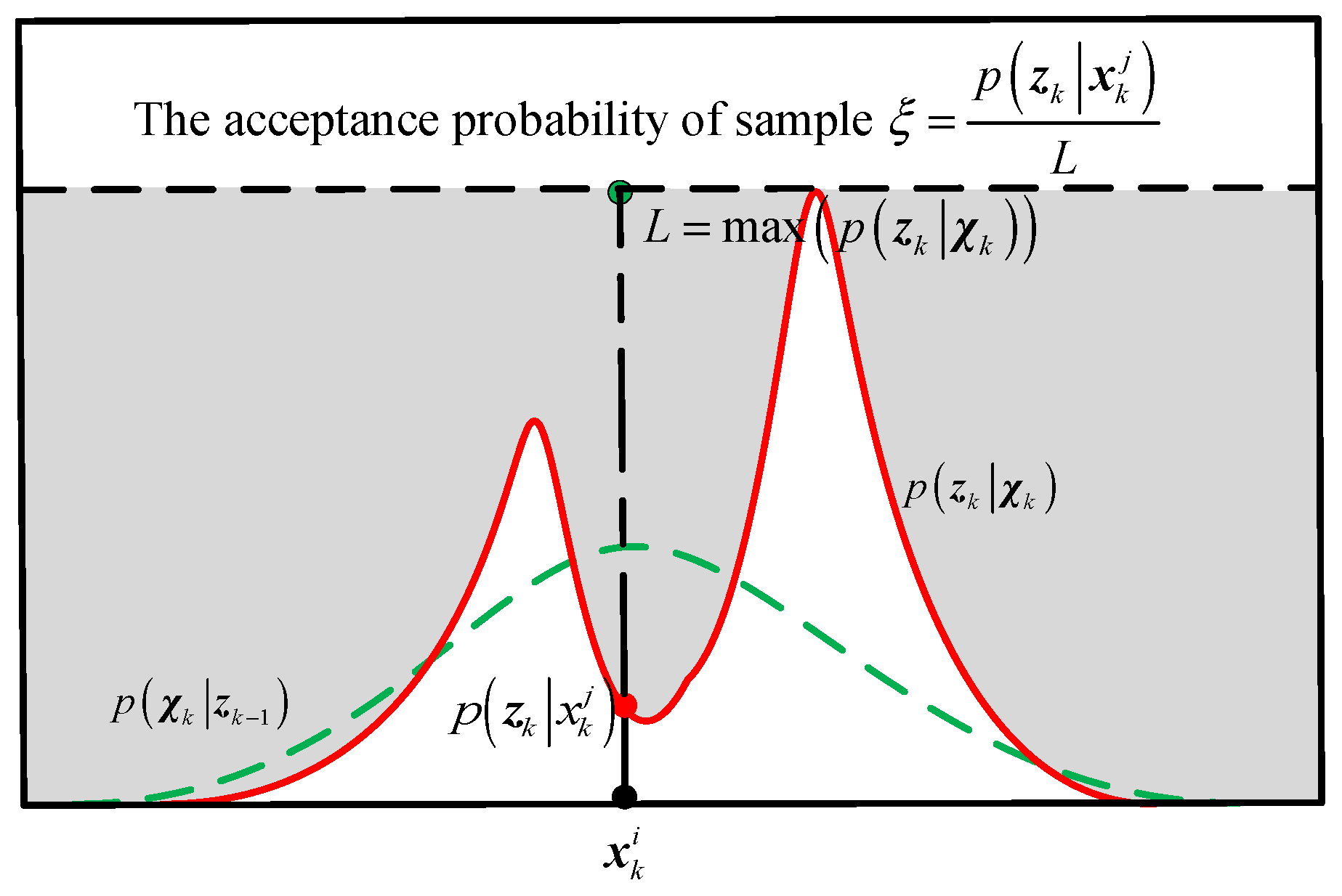
ξ < p z k x k L
where L = M p z k z k 1 . Then, the size of L is to ensure:
L p z k x k         x k d o m p z k x k
In TRN data fusion, since the expression of likelihood distribution is obvious, the selection of L can be calculated simply as follows:
L = max p z k x k
Consequently, the principle of the particle selection method is shown in Figure 7. When we obtain particle x k j from the prior particles X ˜ ˜ k i , we first compute the ratio of its weight to L . We then compare this ratio to a random number ξ to determine whether to reject or accept the particle. The collection of accepted particles forms a particle set X k , which reflects the current posterior distribution p x k z k .
Finally, the state estimation is as follows:
x ^ k = 1 N k i = 1 N k x k i
where X k x k 1 x k 2 x k N k T , x k j denotes a single accepted particle. The detailed BCPS-PF steps are summarized in Algorithm 2.
Algorithm 2. The BCPS-PF algorithm.
Initialization:
Set sample number N 0
Generate the initial sample X 0 N 0 according to the initial PDF p x 0
//Overall time steps:
For k 1 to K do
(1): Obtain the prior particles without state noise model according to X ˜ k = f X k 1 ;
(2): Set i = 1 ; N k = 0 ; X k =
While N k < 0.9 * N 0 :
(3): Obtain a batch of prior particles X ˜ ˜ k i according to Equation (4);
(4): X ˜ ˜ k i are matched with the DEM to generate the predicted observations z k , p r e i ;
(5): Calculate the deviation ε k , p r e i = z k , p r e i z k ;
(6): Calculate the likelihood weights ω ˜ ˜ k i of each particle according to (10);
(7): Generate N k 1 random number ξ i where ξ j i U 0 , 1 ;
For j 1 to N k 1
(8): if ω ˜ ˜ k j i > ξ j i : X k = X k , x ˜ ˜ k j i , N k = N k + 1 ;
End
i = i + 1
End
(9): State estimation according to Equation (13).
End
Remark 1.
In the practical application of The RN system, the observation model is a simple one-dimensional nonlinear system, and the observation noise model is assumed to be a Gaussian noise model. For convenience, the expression of likelihood weights is as follows:
ω ˜ ˜ k i = exp z k z ˜ ˜ k , p r e i 2 2 σ 2
where  σ  is the standard deviation of the observation noise;  z k  is the observation;  z ˜ ˜ k , p r e i  is the predicted observation based on the ith batch of particles. It is easy to know that  max ω ˜ ˜ k i = 1  ; therefore, we can set  L = 1 .
Remark 2.
Due to the uncertainty in selecting the number of particles through RS, it is difficult to precisely obtain  N k 1  particles from the entire cycle of one batch particles. Therefore, the number of particles cannot be fixed in the recursive processing. In this situation, we choose  0.9 × N 0  as the termination condition for the batch cycle. When the number of accepted particles exceeds  0.9 × N 0 , we terminate the batch cycle particle generation mechanism and use the obtained particles as a description of the posterior distribution.

4.3. Computational Complexity Analysis

In terms of computational complexity, BCPS-PF requires O K N d x + d y operations, where N is the target particle count, d x and d y are the state and observation dimensions, and K is the number of acceptance-sampling batches needed to reach a predefined fraction of accepted particles. When the transition prior already overlaps well with the posterior K 1 , BCPS-PF runs in O N d x + d y , matching the cost of SIS-PF. By contrast, EKF-PF and UPF each invoke O N d x 3 per particle (for linearization or sigma-point calculations), resulting in O N d x 3 complexity. Thus, BCPS-PF offers a middle ground: for modest K , its workload remains linear in N and avoids the cubic cost of EKF-PF/UPF, while maintaining better posterior fidelity than SIR-PF.

5. Simulation Experiment

To assess the proposed BCPS-PF algorithm, we consider two representative scenarios: a strongly nonlinear one-dimensional benchmark model and TRN scenarios.

5.1. Kitagawa’s Nonlinear Model

The system model is as follows:
x t = 0.5 x t 1 + 25 x t 1 1 + x t 1 2 + 8 cos 1.2 t 1 + u t 1 y t = 0.05 x t 2 + v t
where the process and observation noise are the Gaussian white noise with zero mean, u t ~ N 0 , σ u 2 , v t ~ N 0 , σ v 2 .
The parameters are set as follows: simulation time T = 50 ; σ v 2 = 0.1 . In addition, we set σ u 2 to two different values—1.0 and 0.1—for evaluating the robustness of BCPS-PF. The initial state is x 0 = 5 , and particles are initialized from a Gaussian prior N x 0 , σ p r i o r 2 with σ p r i o r 2 = 2.0 .
We consider five particle counts: N = 10 , 30 , 50 , 100 , 500 . For each configuration, 500 independent Monte Carlo trials are conducted. Competing algorithms include SIR-PF, EPF, UPF, and APF. BCPS-PF includes a safeguard: if no particles are accepted in a given batch, the particle with the highest likelihood within that batch is retained. This prevents the filter from stalling and ensures continuity in the estimation process under sparse likelihood support. and the number of candidate batches is capped at 50.
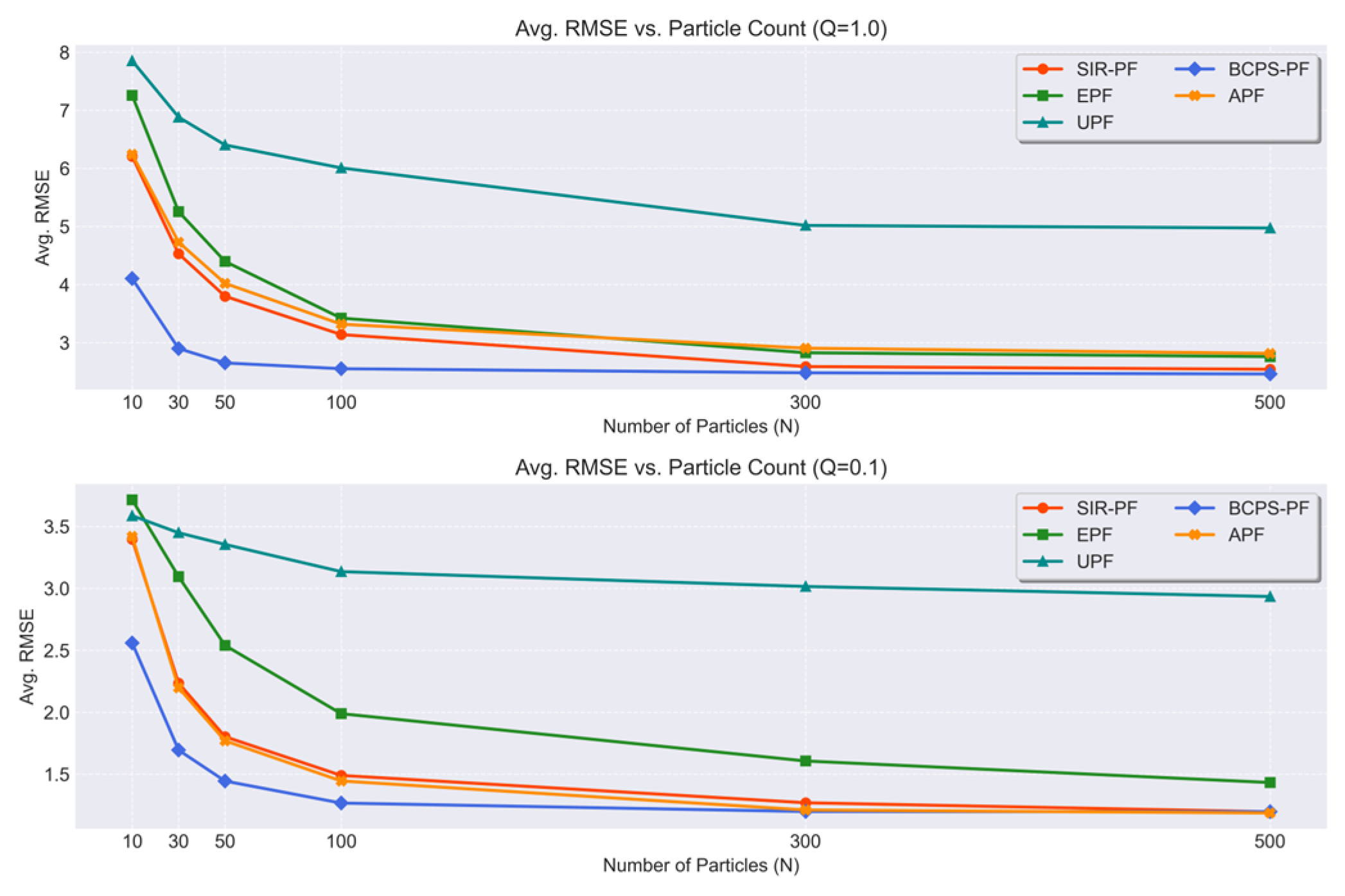
When the variances of process noise and observation noise are at different scales, they can significantly impact the performance of nonlinear filtering algorithms [40]. Figure 8 illustrates the trends in state estimation accuracy for different filtering algorithms as the number of particles increases, under two process noise variance conditions.
As can be seen from Figure 8, the state estimation accuracy of EPF and UPF, which construct their proposal distributions based on linear Gaussian approximations, is weaker than that of SIR-PF, APF, and the proposed BCPS-PF in Kitagawa’s nonlinear model. This is attributed to the fact that, under strong nonlinear conditions, approximations of the noise model often lead to larger errors. Further analysis of the algorithms’ performance under varying process noise covariances reveals instability in the APF compared with the SIR-PF. Specifically, when σ u 2 = 0.1 , the APF improves the filtering accuracy slightly by incorporating likelihood information, demonstrating a superior estimation performance over SIR-PF under equivalent particle counts. However, when σ u 2 = 1.0 , the filtering accuracy of APF paradoxically falls below that of SIR-PF. This performance degradation can be attributed to the dominance of errors introduced by the likelihood information when there is a significant discrepancy between process noise and observation noise, thereby leading to a reduction in filtering accuracy.
In sharp contrast with the aforementioned algorithms, the proposed algorithm is specifically designed to overcome these limitations. It introduces a rejection sampling technique, which indirectly enables the use of an approximate posterior distribution as the proposal distribution. This fundamental approach strictly adheres to the Bayesian filtering framework, eliminates the need for potentially performance-degrading resampling steps, and demonstrates improved convergence in both tested scenarios. Crucially, the BCPS-PF demonstrates significantly improved and consistent estimation accuracy across both tested process noise covariance scenarios. Its stability, regardless of the significant variations in process noise, highlights its robustness against the changing nonlinearity strength and the discrepancy between process and observation noise, unlike the unstable behavior observed in the APF.
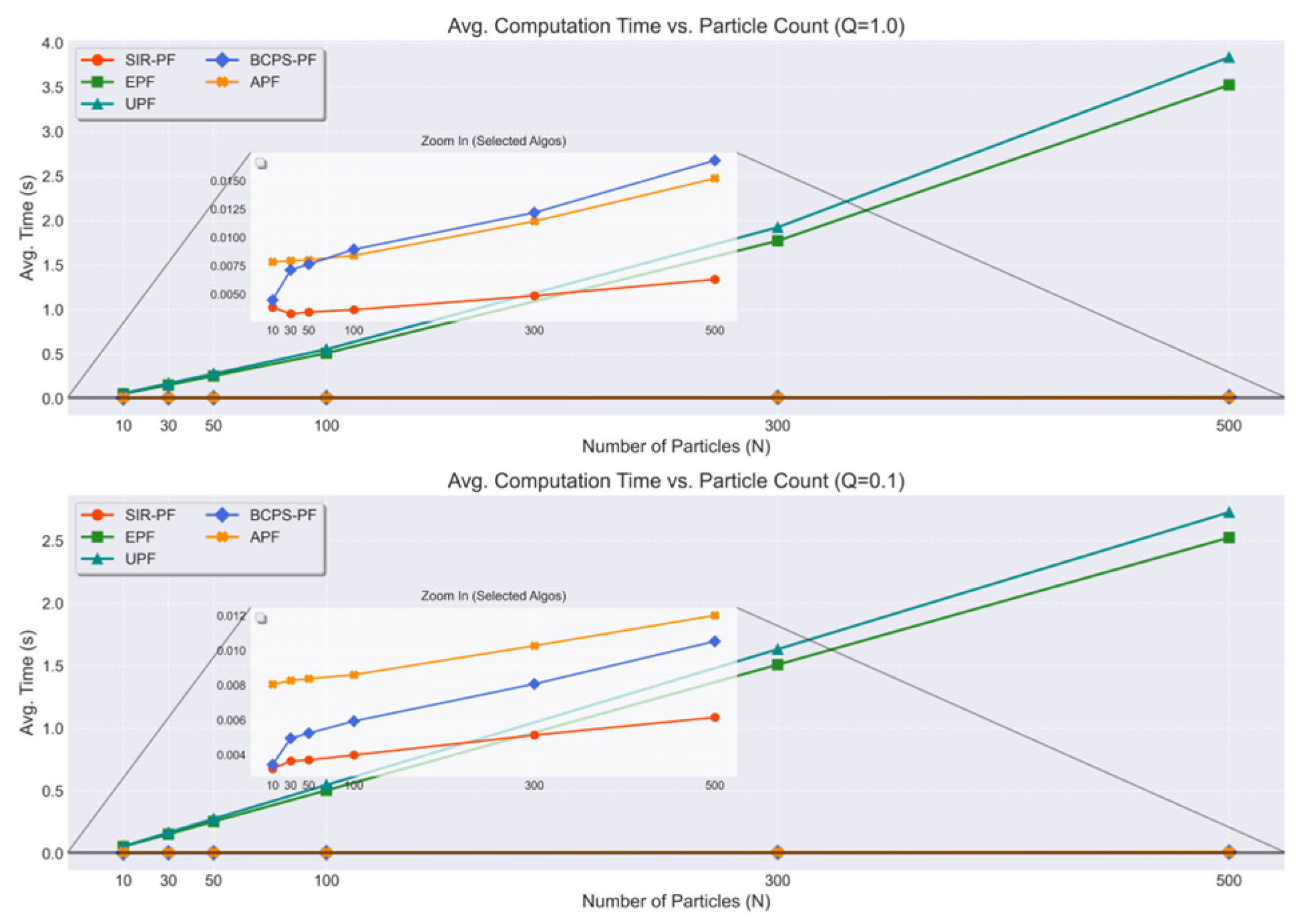
Figure 9 illustrates the computational time required for a single simulation run of different algorithms. As shown in the figure, the computational overhead of the proposed algorithm increases linearly with the increasing number of particles, being slightly higher than that of the SIR-PF algorithm and comparable to APF.

5.2. TRN Scenarios

In this section, simulation experiments are conducted to verify the performance of the BCPS-PF in TRN scenarios.

5.2.1. Simulation Model and Condition

The simulation scenario aims to simulate the process of a UAV flying along a specified trajectory (a figure-eight pattern) in an environment with a loaded DEM. In this scenario, IMU/TRN fusion positioning is performed. The simulation scenario includes the following modules:
(1)
DEM data: The scenario utilizes a pre-loaded DEM with a resolution of 30 m (DEM) [37]. These DEM data are represented by a 4801 × 1000 matrix. The UAV’s initial position for the flight is set at row 87, column 94 within this matrix.
(2)
IMU data: As detailed in Section 2, the mathematical model incorporates errors associated with the IMU’s position and velocity estimations. These errors are modeled as zero-mean Gaussian distributions.
(3)
TRN observation: The TRN observation is obtained by subtracting the barometer altimetry reading from the radar altimetry reading. During this process, independent zero-mean Gaussian distributed errors are introduced for both barometer and radar altimetry measurements.
(4)
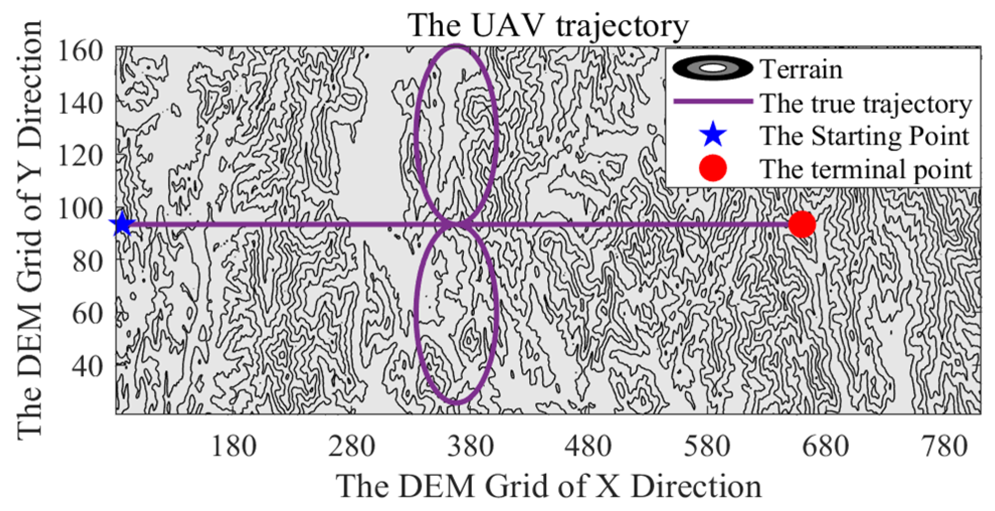
UAV trajectory: The UAV commences its flight from the designated starting point, traveling due east for 86 s at a constant speed. It then performs a northward circular flight for 43 s. Furthermore, it executes another southward circular flight for 43 s. Finally, it flies straight towards the east for 128 s. The total flight time is 300 s. Throughout the entire flight, the UAV maintains a constant speed. The trajectory of the UAV flying over the DEM is shown in Figure 10. The relevant parameters are shown in Table 1.

5.2.2. Method

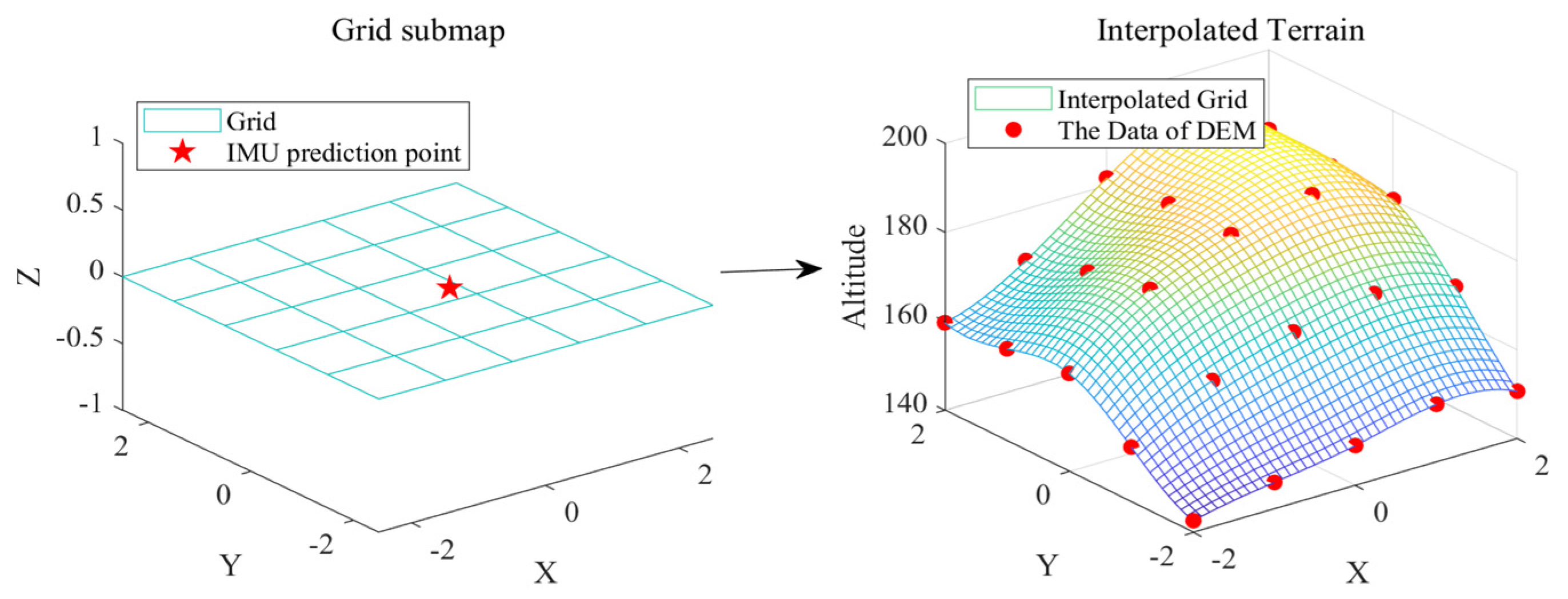
To evaluate the performance of the proposed IMU/TRN fusion localization algorithm, we employed the aforementioned simulation scenario. In this scenario, the state transition function is provided by the IMU, and the observation equation is determined by the observation and the matching status with the DEM. See Section 2 for details. The specific matching process is as follows: First, the prior position estimation result was provided by the IMU, and the data of the two adjacent grids (60 m extension) around the position were selected as the DEM submap based on the prior position, and the submap was linearly interpolated as the matching object, as shown in Figure 11. Additionally, we compared the BCPS-PF against four nonlinear filtering methods: PF, auxiliary PF (APF), mixture particle filter (MPF), and OOSM-PF. All particle filter-based algorithms utilized the sampling importance resampling (SIR) method and set the number of particles to 500. For BCPS-PF, it was difficult to precisely maintain a fixed number of particles during the multi-batch particle selection process. Therefore, we set the initial number of particles to 500 and employed a threshold of 450 particles for termination in the recursive iteration. When the number of particles exceeded 450, the loop was terminated, and state estimation was performed. Moreover, the BCPS-PF directly generated particles that satisfied the posterior distribution diversity, eliminating the need for resampling. Finally, we conducted 100 Monte Carlo experiments for the IMU/TRN fusion localization process and employed the minimum mean squared error (MSE) as the metric to evaluate state estimation accuracy, as follows:
R M S E p x = 1 M o n t e r m = 1 M o n t e r p k x p ^ k x 2
R M S E p y = 1 M o n t e r m = 1 M o n t e r p k y p ^ k y 2
R M S E = 1 M o n t e r m = 1 M o n t e r p k x p ^ k x 2 + p k y p ^ k y 2
where R M S E p x and R M S E p y denote the RMSE of east–west and north–south directions, respectively. p k x and p k y denote the real position on east–west and north–south directions at time step k , respectively. p ^ k x and p ^ k y denote the results of the state estimation of position on east–west and north–south directions at time step k , respectively. M o n t e r denotes the number of Monte Carlo runs.

5.2.3. Results

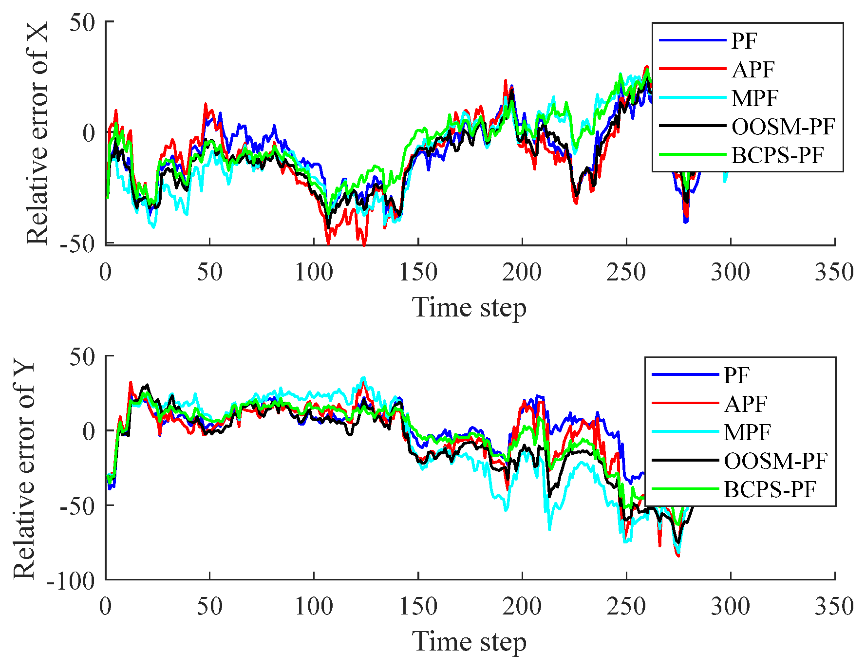
Figure 12 and Figure 13 present the outcomes of a simulation experiment conducted within this scenario. As illustrated in Figure 12, our proposed algorithm and the four comparison algorithms successfully achieve IMU/TRN data fusion. Figure 13 highlights the posterior particle distributions of the different algorithms after fusion at the 251st time step, while the ✯ represent the true position. In this figure, the pentagram indicates the UAV’s actual position at the current moment, and subplot (f) shows the real posterior distribution. It is evident that the high-probability region of the posterior distribution deviates significantly from the real position due to the substantial observation noise at this time, which creates a disparity between the likelihood distribution and the prior distribution. This discrepancy results in a high-probability region of the posterior distribution that is far from the real position. Nevertheless, the goal remains to have particles that more accurately reflect the posterior distribution to achieve an optimal state estimation from a probabilistic statistical perspective.
Subplots (a) to (e) provide further insights: the APF algorithm’s particles are more concentrated in the upper right because this method emphasizes the weight of observation information, leading the particles to cluster in the high-probability region of the likelihood distribution. Although the PF algorithm does not emphasize the weight of observation information, the significant difference between the likelihood distribution and the prior distribution causes many particles to replicate in the high-probability region of the likelihood distribution. The MPF algorithm’s particles show a tendency to migrate toward the high-probability region of the posterior distribution; however, since its proposal distribution is not the accurate posterior distribution, the particles remain more dispersed. The OOSM-PF algorithm’s state estimation is closest to the true state because it detects when the likelihood distribution deviates significantly from the prior distribution and considers such observations as ambiguous, thus discarding them. However, from a statistical standpoint, a significant deviation between the likelihood observation and the prior distribution does not necessarily indicate reduced observation quality. Therefore, this strategy may not always be optimal. In contrast, the particle distribution of our proposed algorithm aligns most closely with the true posterior distribution. By utilizing particle flow generation and particle flow selection mechanisms, the proposed algorithm can directly generate particles that satisfy the posterior distribution without being affected by the degradation or lack of diversity related to the proposal distribution’s proximity to the posterior distribution.
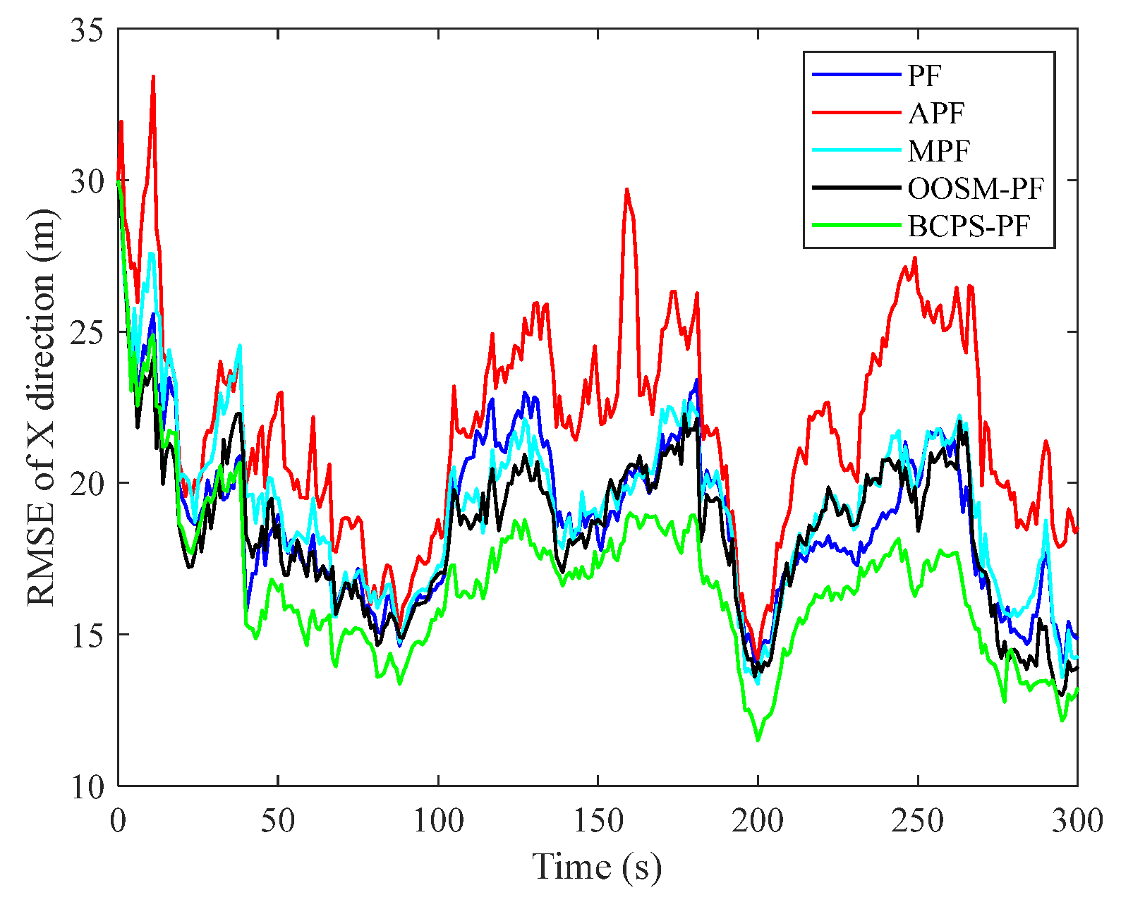
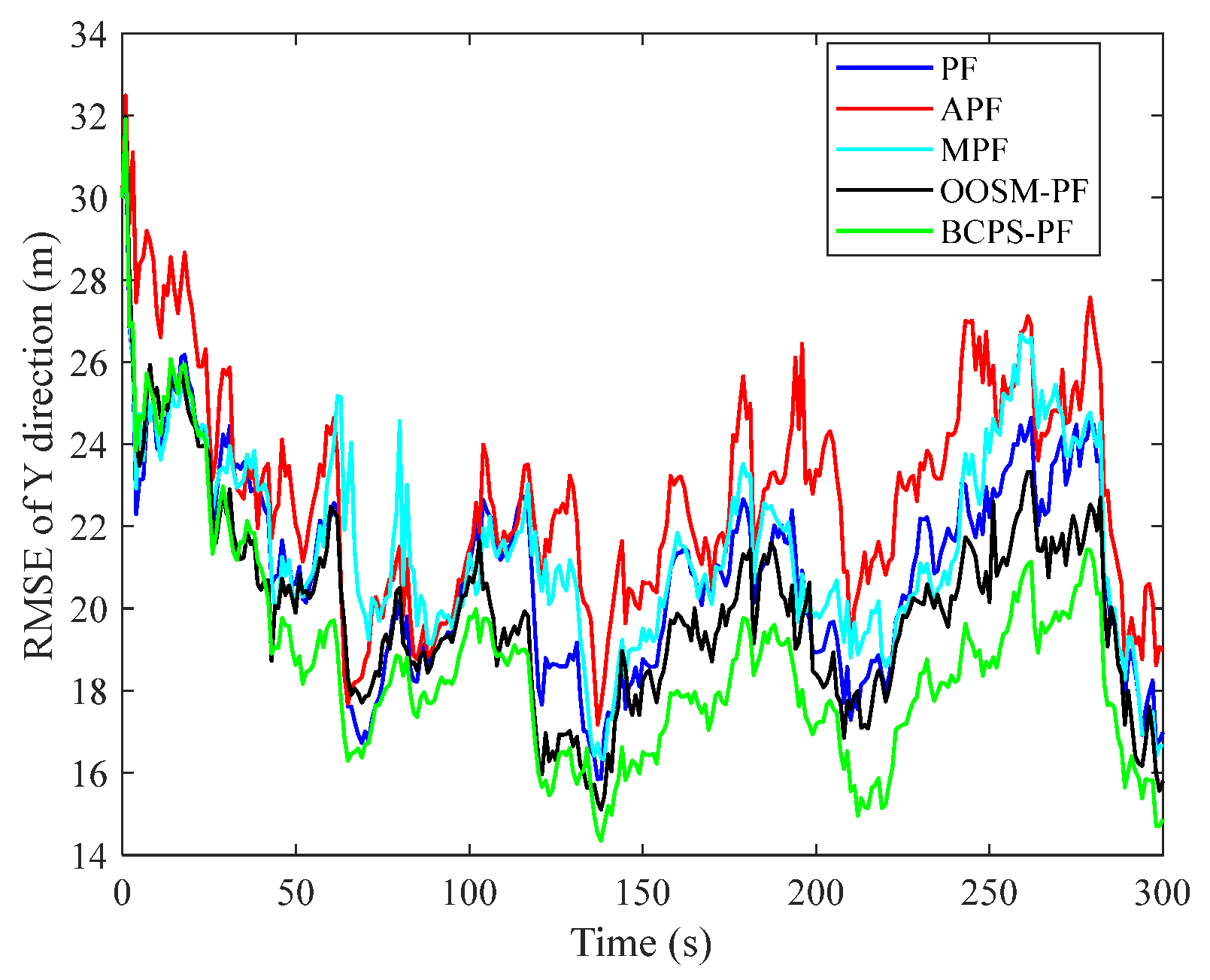
The results of 100 Monte Carlo simulations for this scenario are presented in Figure 14, Figure 15 and Figure 16. Figure 14 and Figure 15 show the root mean square error (RMSE) of the positioning results for five filter algorithms in two directions. Compared with other PF-based algorithms, the APF relies more heavily on the observation model. However, the observation model of TRN generates a multimodal likelihood distribution, which statistically reduces the fusion accuracy of the APF. Both PF and the MPF algorithm achieve similar fusion accuracy because the clustering mode based on mixed Gaussians used in MPF is not well-suited for multimodal distributions in TRN environments. Consequently, the enhancements introduced by MPF over PF do not provide significant benefits in this scenario. OOSM-PF achieves slightly higher fusion accuracy than MPF and PF due to its better adaptability to the characteristics of TRN scenarios. The BCPS-PF, which directly generates particles that satisfy the posterior distribution, results in superior fusion accuracy compared with the benchmark algorithms.
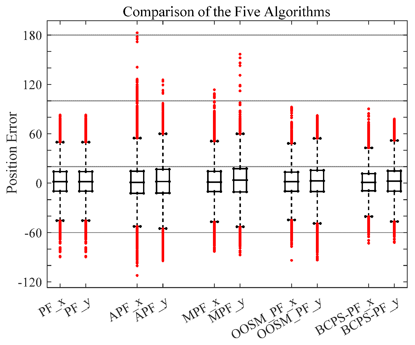
Figure 16 presents a statistical analysis of the positioning errors from 100 rounds of Monte Carlo simulations. The interquartile range (IQR) of the upper and lower quartiles for all five methods is relatively similar, with the proposed algorithm having a slightly smaller IQR. The number and range of outliers for APF and MPF are significantly higher compared with the other three methods. This further validates that the improvements introduced by APF and MPF to particle filtering are not well-suited for TRN scenarios, leading to decreased system stability. Additionally, the number and magnitude of outliers observed for PF, OOSM-PF, and the proposed algorithm are relatively similar. The superior fusion accuracy of the proposed algorithm is attributed to its smaller IQR, resulting from its particles providing a more accurate representation of the posterior distribution.
Table 2 presents the RMSE results for different algorithms over the entire time steps. The novel particle filter using the posterior distribution as the proposal distribution demonstrates a superior RMSE performance compared with the other filter algorithms. When ambiguous observations are detected and excluded, the RMSE performance of the OOSM algorithm slightly surpasses that of the standard particle filter. In contrast, the APF algorithm shows the poorest performance due to its excessive reliance on observations. The standard particle filter has the lowest time cost, while the time costs of the APF and the novel particle filter are similar. Notably, the positioning accuracy of the novel particle filter is improved by 10% compared with the standard particle filter.

6. Conclusions

In this paper, we addressed the challenges associated with the multimodal distribution of elevation observations in terrain referenced navigation (TRN). The fluctuating nature of terrain introduces uncertain noise probability distributions, making nonlinear filtering methods more suitable for fusing TRN and IMU data. Traditional PF often suffers from poor accuracy and robustness due to the difficulty in balancing particle degradation and diversity. To tackle these issues, we developed BCPS-PF, which indirectly uses the posterior distribution as the proposal distribution. This approach eliminates the need for resampling and bypasses the requirement to propagate weights during the recursive Bayesian update. Instead, it relies solely on particles that satisfy the posterior distribution to accurately estimate the current state. Our proposed algorithm was specifically adapted for TRN applications. Simulations demonstrated its effectiveness, showing a 10% improvement in positioning accuracy compared with existing algorithms. This significant enhancement underscores the algorithm’s potential for improving the reliability and precision of TRN systems.

Author Contributions

Conceptualization, Z.L. and X.Q.; methodology, W.S.; software, Y.G.; validation, resources, L.W.; visualization, Z.L. and X.Q. All authors have read and agreed to the published version of the manuscript.

Funding

This work was supported by the National Natural Science Foundation of China (Grant No. 62303007), the Doctoral Research Start-up Funding (Grant No. S020318015/028) of Anhui University and the Open Project Program of State Key Laboratory of CNS/ATM, China (No.2024B22).

Data Availability Statement

The data presented in this study are available on request from the corresponding author due to the fact that this research is part of an ongoing long-term project.

Conflicts of Interest

Author Wenwu Shi was employed by the company IKD New Energy Automotive Parts Company Limited. The remaining authors declare that this research was conducted in the absence of any commercial or financial relationships that could be construed as a potential conflict of interest.

References

  1. Vaman, D. TRN history trends and the unused potential. In Proceedings of the IEEE/AIAA 31st Digital Avionics Systems Conference, Williamsburg, VA, USA, 14–18 October 2012; pp. 1A3-1–1A3-16. [Google Scholar]
  2. Kim, Y.; Park, J.; Bang, H. Terrain-referenced navigation using an interferometric radar altimeter. Navigation 2018, 65, 157–167. [Google Scholar] [CrossRef]
  3. Carroll, J.D.; Canciani, A.J. Terrain-referenced navigation using a steerable-laser measurement sensor. Navigation 2021, 68, 115–134. [Google Scholar] [CrossRef]
  4. Yin, J.; Zhang, J.; Klaas, M. The Marginal Rao-Blackwellized Particle Filter for Mixed Linear/Nonlinear State Space Models. Chin. J. Aeronaut. 2007, 20, 346–352. [Google Scholar] [CrossRef]
  5. Copp, B.; Subbarao, K. Nonlinear adaptive filtering in terrain-referenced navigation. IEEE Trans. Aerosp. Electron. Syst. 2015, 51, 3461–3469. [Google Scholar] [CrossRef]
  6. Choe, Y.; Park, C.G. Point-mass filtering with boundary flow and its application to terrain referenced navigation. IEEE Trans. Aerosp. Electron. Syst. 2021, 57, 3600–3613. [Google Scholar] [CrossRef]
  7. Liu, D.; Chen, X.; Liu, X. A novel optimal data fusion algorithm and its application for the integrated navigation system of missile. Chin. J. Aeronaut. 2022, 35, 53–68. [Google Scholar] [CrossRef]
  8. Ahwiadi, M.; Wang, W. An adaptive particle filter technique for system state estimation and prognosis. IEEE Trans. Instrum. Meas. 2020, 69, 6756–6765. [Google Scholar] [CrossRef]
  9. Zhu, N.; Zhao, H.; Feng, W.; Wang, Z. A novel particle filter approach for indoor positioning by fusing WiFi and inertial sensors. Chin. J. Aeronaut. 2015, 28, 1725–1734. [Google Scholar] [CrossRef]
  10. Wan, X.; Shao, Y.; Zhang, S.; Li, S. Terrain aided planetary UAV localization based on geo-referencing. IEEE Trans. Geosci. Remote Sens. 2022, 60, 1–18. [Google Scholar] [CrossRef]
  11. Qiang, X.; Zhu, Y.; Xue, R. SVRPF: An Improved Particle Filter for a Nonlinear/Non-Gaussian Environment. IEEE Access 2019, 7, 151638–151651. [Google Scholar] [CrossRef]
  12. Zhao, L.; Gao, N.; Huang, B.; Wang, Q.; Zhou, J. A novel terrain-aided navigation algorithm combined with the TERCOM algorithm and particle filter. IEEE Sens. J. 2014, 15, 1124–1131. [Google Scholar] [CrossRef]
  13. Talebi, S.P.; Mandic, D.P. Distributed Particle Filtering of-Stable Signals. IEEE Signal Process. Lett. 2017, 24, 1862–1866. [Google Scholar] [CrossRef]
  14. Golden, J.P. Terrain contour matching (TERCOM): A cruise missile guidance aid. In Image Processing for Missile Guidance; SPIE: Bellingham, WA, USA, 1980; Volume 238, pp. 10–18. Available online: https://www.spiedigitallibrary.org/conference-proceedings-ofspie/0238/0000/Terrain-Contour-Matching-TERCOM-A-Cruise-Missile-Guidance-Aid/10.1117/12.959127.full (accessed on 29 September 2025).
  15. Baker, W.; Clem, R. Terrain Contour Matching [TERCOM] Primer; Technical Report ASP-TR-77-61; Aeronautical Syst. Division, Wright-Patterson AFB, Wright-Patterson Air Force Base: Dayton, OH, USA, 1977. [Google Scholar]
  16. Hollowell, J. Heli/SITAN: A Terrain Referenced Navigation Algorithm for Helicopters. January 1990. Available online: https://www.osti.gov/biblio/5127167 (accessed on 29 September 2025).
  17. Boozer, D.D.; Fellerhoff, J.R. Terrain-aided navigation test results in the AFTI/F-16 aircraft. Navigation 1988, 35, 161–175. [Google Scholar] [CrossRef]
  18. Wei, E.; Dong, C.; Yang, Y.; Tang, S.; Liu, J.; Gong, G.; Deng, Z. Arobust solution of integrated SITAN with TERCOM algorithm: Weightreducing iteration technique for underwaterVehicles’ gravity-aided inertial navigation system. Navigation 2017, 64, 111–122. [Google Scholar] [CrossRef]
  19. Peng, H.Z.; Jun, Y.; Wei, W.W.; Zhi, M.B. An algorithm of terrain matching aided navigation forUAVs. In Proceedings of the IEEE CSAA Guidance, Navigation and Control Conference (CGNCC), Xiamen, China, 10–12 August 2018; pp. 1–6. [Google Scholar]
  20. Cowie, M.; Wilkinson, N.; Powlesland, R. Latest development of the TERPROM digital terrain system (DTS). In Proceedings of the IEEE/ION Position, Location and Navigation Symposium, Monterey, CA, USA, 5–8 May 2008; pp. 1219–1229. [Google Scholar]
  21. Yuan, G.; Zhang, H.; Yuan, K.; Zhu, L. Improved SITAN algorithm in the application of aided inertial navigation. In Proceedings of the International Conference on Measurement, Information and Control, Vinnytsia, Ukraine, 9–11 October 2012; Volume 2, pp. 922–926. [Google Scholar]
  22. Oh, J.; Sung, C.K.; Lee, J.; Lee, S.W.; Lee, S.J.; Yu, M.J. Accurate measurement calculation method for interferometric radar altimeter-based terrain referenced navigation. Sensors 2019, 19, 1688. [Google Scholar] [CrossRef]
  23. Enns, R.; Morrell, D. Terrain-aided navigation using the Viterbi algorithm. J. Guid. Control Dyn. 1995, 18, 1444–1449. [Google Scholar] [CrossRef]
  24. Ånonsen, K.B. Advances in Terrain Aided Navigation for Underwater Vehicles. Ph.D. Thesis, Department of Engineering Cybernetics, Norwegian University of Science and Technology, Trondheim, Norway, 2010. [Google Scholar]
  25. Bergman, N.; Ljung, L.; Gustafsson, F. Terrain navigation using Bayesian statistics. IEEE Control Syst. 1999, 19, 33–40. [Google Scholar]
  26. Park, Y.-G.; Park, C.G. Grid support adaptation for point mass filter-based terrain referenced navigation using mutual information. IEEE Sens. J. 2018, 18, 7603–7610. [Google Scholar] [CrossRef]
  27. Zhang, K.; Li, Y.; Zhao, J.; Rizos, C. A Study of Underwater Terrain Navigation based on the Robust Matching Method. J. Navig. 2014, 67, 569–578. [Google Scholar] [CrossRef]
  28. Ma, T.; Ding, S.; Li, Y.; Fan, J. A review of terrain aided navigation for underwater vehicles. Ocean. Eng. 2023, 281, 114779. [Google Scholar] [CrossRef]
  29. Ristic, B.; Arulampalam, S.; Gordon, N. Beyond Kalman Filter: Particle Filters for Tracking Applications; Artech House: Norwood, MA, USA, 2003. [Google Scholar]
  30. Gustafsson, F.; Gunnarsson, F.; Bergman, N.; Forssell, U.; Jansson, J.; Karlsson, R.; Nordlund, P.J. Particle filters for positioning, navigation, and tracking. IEEE Trans. Signal Process. 2002, 50, 425–437. [Google Scholar] [CrossRef]
  31. Nordlund, P.-J.; Gustafsson, F. Marginalized particle filter for accurate and reliable terrain-aided navigation. IEEE Trans. Aerosp. Electron. Syst. 2009, 45, 1385–1399. [Google Scholar] [CrossRef]
  32. Turan, B. Comparison of nonlinear filtering methods for terrain referenced aircraft navigation. In Proceedings of the IEEE/ION Position, Location and Navigation Symposium (PLANS), Portland, OR, USA, 20–23 April 2020; pp. 144–149. [Google Scholar]
  33. Turan, B.; Kutay, A.T. Particle filter studies on terrain referenced navigation. In Proceedings of the IEEE/ION Position, Location and Navigation Symposium (PLANS), Savannah, GA, USA, 11–14 April 2016; pp. 949–954. [Google Scholar]
  34. Salavasidis, G.; Munafò, A.; McPhail, S.D.; Harris, C.A.; Fenucci, D.; Pebody, M.; Rogers, E.; Phillips, A.B. Terrain-aided navigation with coarse maps—Toward an Arctic crossing with an AUV. IEEE J. Ocean. Eng. 2021, 46, 1192–1212. [Google Scholar] [CrossRef]
  35. Palmier, C.; Dahia, K.; Merlinge, N.; Del Moral, P.; Laneuville, D.; Musso, C. Adaptive approximate Bayesian computational particle filters for underwater terrain aided navigation. In Proceedings of the 22th International Conference on Information Fusion (FUSION), Ottawa, ON, Canada, 2–5 July 2019; pp. 1–8. [Google Scholar]
  36. Li, X.; Zhong, Y.; Han, Y. Constrained cubature particle filter for vehicle navigation. Sensors 2024, 24, 1228. [Google Scholar] [CrossRef] [PubMed]
  37. Jia, K.; Pei, Y.; Gao, Z.; Zhong, Y.; Gao, S.; Wei, W.; Hu, G. A Quaternion-Based Robust Adaptive Spherical Simplex Unscented Particle Filter for MINS/VNS/GNS Integrated Navigation System. Math. Probl. Eng. 2019, 2019, 8532601. [Google Scholar] [CrossRef]
  38. Zhou, T.; Wang, T.; Gao, J.; Guo, Q.; Yan, Z. Particle filter underwater terrain-aided navigation based on gradient fitting. Meas. Sci. Technol. 2022, 33, 105009. [Google Scholar] [CrossRef]
  39. Qiang, X.; Xue, R.; Zhu, Y. Bayesian filter based on grid filtration and its application to Multi-UAV tracking. Signal Process. 2022, 190, 108305. [Google Scholar] [CrossRef]
  40. Dissanayaka, D.; Wanasinghe, T.R.; De Silva, O.; Jayasiri, A.; Mann, G.K.I. Review of Navigation Methods for UAV-Based Parcel Delivery. IEEE Trans. Autom. Sci. Eng. 2024, 21, 1068–1082. [Google Scholar] [CrossRef]
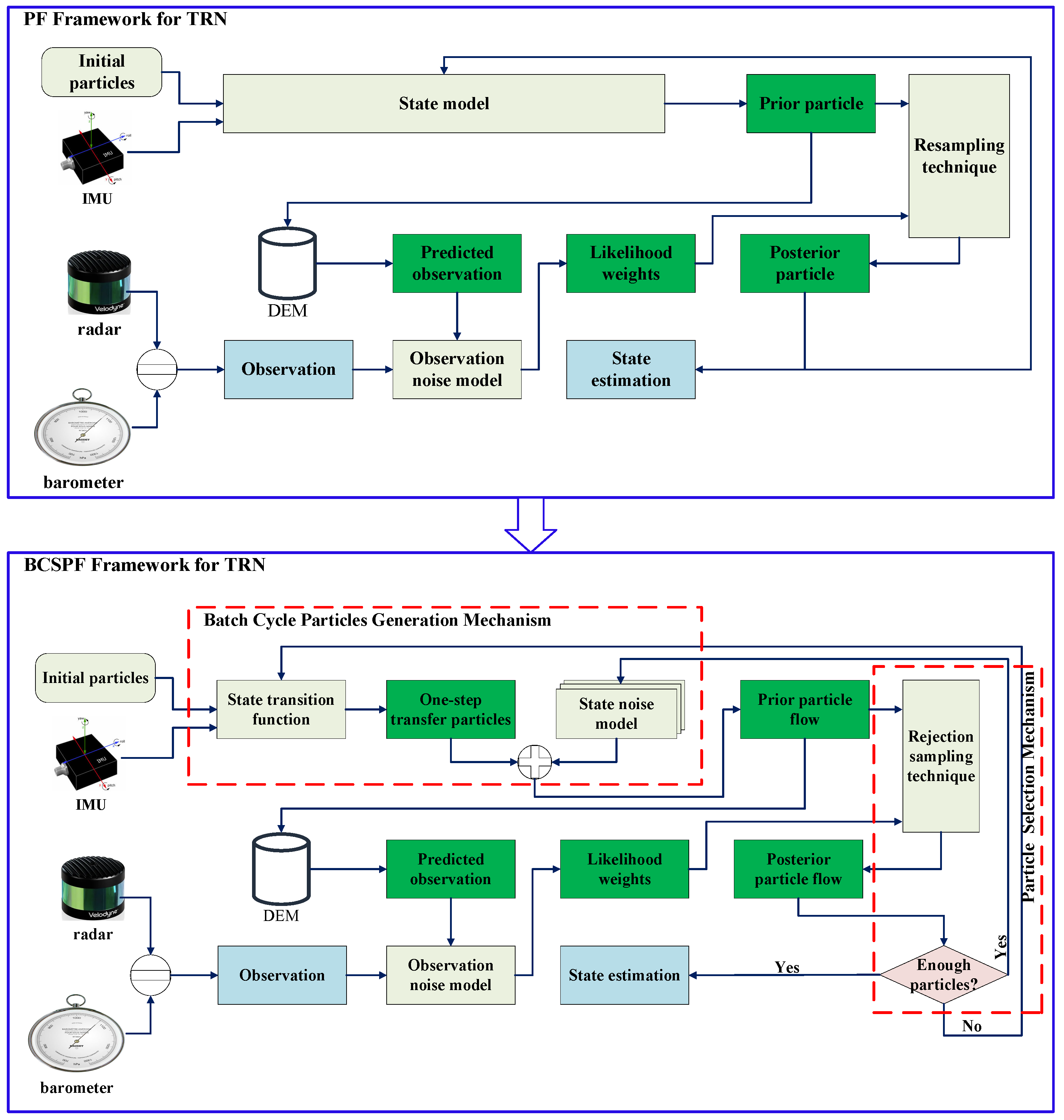
Figure 1. The framework of BCPS-PF compared with PF for IMU/TRN fusion.
Electronics 14 04257 g001
Figure 2. The principle of TRN measurement acquisition.
Electronics 14 04257 g002
Figure 3. The schematic diagram of probability information transfer.
Electronics 14 04257 g003
Figure 4. Decomposition of the state transition function with the state noise model.
Electronics 14 04257 g004
Figure 5. Schematic diagram of batch cycle particle generation.
Electronics 14 04257 g005
Figure 6. Schematic diagram of observations showing a multimodal distribution.
Electronics 14 04257 g006
Figure 7. The principle of particle selection.
Electronics 14 04257 g007
Figure 8. The variation of the average RMSE with the number of particles under different process noise conditions.
Electronics 14 04257 g008
Figure 9. The variation of the single filtering time cost with the number of particles under different process noise conditions.
Electronics 14 04257 g009
Figure 10. The trajectory of the UAV flying over the DEM.
Electronics 14 04257 g010
Figure 11. The diagram of DME submap acquisition and its interpolation.
Electronics 14 04257 g011
Figure 12. The relative error of two directions for the positioning results.
Electronics 14 04257 g012
Figure 13. The particle distribution of different fusion algorithms at time step 251.
Electronics 14 04257 g013
Figure 14. The RMSE of X direction according to the time step.
Electronics 14 04257 g014
Figure 15. The RMSE of Y direction according to the time step.
Electronics 14 04257 g015
Figure 16. Positioning error box diagram of different fusion positioning algorithms.
Electronics 14 04257 g016
Table 1. The parameter configuration of simulation.
ConditionValue
Simulation duration300 s
Velocity100 m/s
The flight altitude900 m
Initial position error40 m
The std of position error estimated by the IMU5
The std of velocity error estimated by the IMU2
IMU sampling frequency1 Hz
The flight altitude900 m
Observation sampling frequency1 Hz
The std of observation error obtained by barometer altimetry15
The std of observation error obtained by radar altimetry4.71
Table 2. The performance of difference of filter algorithms in terms of RMSE and time cost.
MethodRMSETimes(s)
X Y X Y --
PF22.527625.079633.78860.0463
APF26.271627.407738.06660.0924
MPF23.083025.836034.71220.9856
OOSM22.074124.005532.68980.0736
BCPS-PF20.028022.490930.18380.0838
Disclaimer/Publisher’s Note: The statements, opinions and data contained in all publications are solely those of the individual author(s) and contributor(s) and not of MDPI and/or the editor(s). MDPI and/or the editor(s) disclaim responsibility for any injury to people or property resulting from any ideas, methods, instructions or products referred to in the content.